On Safety and Liveness Filtering Using Hamilton-Jacobi Reachability Analysis
Abstract
Hamilton-Jacobi (HJ) reachability-based filtering provides a powerful framework to co-optimize performance and safety (or liveness) for autonomous systems. Under this filtering scheme, a nominal controller is minimally modified to ensure system safety or liveness. However, the resulting controllers can exhibit abrupt switching and bang-bang behavior, which is not suitable for applications of autonomous systems in the real world. This work presents a novel, unifying framework to design safety and liveness filters through reachability analysis. We explicitly characterize the maximal set of control inputs that ensures safety (or liveness) at a given state. Different safety filters can then be constructed using different subsets of this maximal set along with a projection operator to modify the nominal controller. We use the proposed framework to design three safety filters, each balancing performance, computation time, and smoothness differently. The proposed filters can easily handle dynamics uncertainties, disturbances, and bounded control inputs. We highlight their relative strengths and limitations by applying these filters to autonomous navigation and rocket landing scenarios and on a physical robot testbed. We also discuss practical aspects associated with implementing these filters on real-world autonomous systems. Our research advances the understanding and potential application of reachability-based controllers on real-world autonomous systems.
Index Terms:
Robot Safety, Reachability Analysis, Safety Filtering.I Introduction
As autonomous systems become integral to our daily lives, it is crucial to design controllers that are both safe and performant. Typically, controller design is framed as an optimal control problem, balancing performance criteria (e.g., minimizing control energy), with safety constraints, such as obstacle avoidance. The resultant constrained optimal control problem is solved using a variety of methods ranging from Model Predictive Control (MPC) [25, 11, 8] and (approximate) dynamic programming [6, 7] to data-driven, reinforcement learning approaches [14, 23]. Despite impressive performance of these methods, ensuring hard safety constraints for general, nonlinear systems remains a challenge, especially if the optimal control problem needs to be solved online.
An alternative approach is safety filtering, where a nominal control input (often performance-oriented) is minimally adjusted (i.e., “filtered”) to satisfy the safety constraint. If the input is safe, it is used directly; otherwise, it is projected to a set of safe control inputs. This approach guarantees safety while optimizing performance whenever the system safety is not at risk. Akin to safety filters, one can also design liveness filters, which ensure that the system reaches a desired set of states (e.g., the landing pad for a rocket) within a set timeframe while optimizing the performance (e.g., minimizing the control energy).
A number of approaches have been proposed in literature to construct safety and liveness filters for dynamical systems, such as Control Barrier and Control Lyapunov functions, Hamilton-Jacobi reachability, and MPC. We discuss some of the relevant approaches here and refer the interested readers to [13] and [24] for a detailed survey on filtering methods.
Hamilton-Jacobi (HJ) reachability analysis [17, 19] is a popular mechanism to design these filters due to its ability to ensure safety and liveness for dynamical systems with general nonlinear dynamics, control bounds, and disturbances [18, 4, 5]. In reachability analysis, one is interested in computing the backward reachable tube (BRT) of a dynamical system, i.e. the set of all initial states from which the system will eventually reach a target set, despite the worst case disturbance. Thus, if the target set represents the set of desirable states (e.g., goal states for a vehicle), the BRT represents the set of states from which liveness can be guaranteed. Conversely, if the target set represents the set of undesirable states (e.g., obstacles), the BRT contains states which are potentially unsafe for the system and should therefore be avoided. Alongside the BRT, reachability analysis provides a safety controller (respectively liveness controller) that will provably steer the system away from the target set (respectively towards the target set). A simple safety filter uses the BRT and safety controller: the system employs the nominal controller outside the BRT and switches to the reachability safety controller at the BRT boundary, ensuring constant safety. However, controllers from HJ reachability are often extremum seeking, resulting in a bang-bang behavior. This behavior along with a sudden switching between the nominal and reachability controllers leads to jittery state and control trajectories, which is often undesirable for real-world autonomous systems [24].
An alternative approach to filtering involves using Control Barrier Functions (CBF) for safety and Control Lyapunov Functions (CLF) for liveness filtering. Both utilize Lyapunov-like conditions to ensure the forward invariance of a set [2], which then aids in creating a quadratic program (QP) for a smooth blending of nominal and safety (or liveness) controllers. However, despite recent progress [9, 22, 21, 26], constructing a valid Lyapunov or barrier function for general nonlinear systems with control bounds and disturbances remains a challenge. Some recent studies have addressed this by framing CBF synthesis as an HJ reachability problem, capitalizing on the constructive attributes of reachability methods for obtaining a valid CBF [9]. The resultant CBF can be used for smooth, QP-based controller synthesis. However, a few questions remain: can we derive smooth control laws directly from reachability analysis without constructing a CBF first? How do these safety filters compare in performance and computation? And can we design such control laws for liveness filtering?
In this work, we answer the aforementioned questions in affirmative and introduce a general framework to design safety and liveness filters using reachability analysis. Under the proposed framework, any safety and liveness filter can be thought of as a combination of two components: (a) a projection set – a set of safe or live control inputs that the nominal controller will be projected to; and (b) a projection operator to align a nominal control input with this set. Drawing on this insight, our key idea is to use HJ reachability analysis to explicitly characterize the set of all possible control inputs at a state that guarantees system safety or liveness. Various safety filters can then be obtained by using different subsets of this maximal safe control set as the projection set, along with a projection operator. Building upon this framework, we propose three different safety and liveness filters based on reachability analysis: a least restrictive safety filter, a smooth least restrictive filter, and a smooth blending filter. The proposed filters are versatile, applicable to both liveness and safety, accommodating control bounds, adversarial disturbances, model uncertainties, and time-specific liveness and safety properties (e.g., reach the target set within 5 seconds). We further compare these filters on various metrics including performance, computation time, controller tuning, and control profile smoothness, and highlight the key trade-offs. Beyond these specific filters, our approach provides a unifying framework for existing reachability-based filters and designing new ones using diverse subsets of the maximal safe set and projection operators. We showcase our approach in two different applications inspired by rocket landing within a given landing window and safe autonomous blimp navigation, as well as on a physical robot testbed involving a wheeled robot navigating through a cluttered environment.
II Problem Statement
Consider an autonomous system with state that evolves according to dynamics
| (1) |
where and are the control and disturbance of the system, respectively. can represent potential model uncertainties or an actual, adversarial exogenous input to the system. We assume the dynamics is uniformly continuous, bounded, and Lipschitz continuous in for fixed and ; such an assumption guarantees that a unique system trajectory would solve (1) [10] for all initial states. Finally, let denote the system state at time , starting from the state at time under control input and disturbance signal while following the dynamics (1). A control input is defined as a measurable function mapping from the time horizon to the set of admissible controls , and a disturbance signal is similarly defined.
In this work, we are interested in synthesizing, potentially time-varying, controllers that steer the system to reach (liveness) or avoid (safety) a given target set , within the time horizon . can represent the goal region in the case of liveness or an unsafe region of the state space in the case of safety, e.g., obstacles for a navigation robot. Furthermore, we would like our controllers to consider other performance objectives while guaranteeing liveness/safety. We assume the performance objectives are encoded and optimized by an user-defined nominal controller . However, may not necessarily ensure liveness (or safety). Our goal is to design to follow to the extent possible, while guaranteeing liveness/safety requirement.
One popular mechanism to achieve this goal is liveness or safety filtering, in which is modified minimally to ensure system liveness or safety [3, 4]. In this paper, we will leverage reachability analysis to synthesize such filters.
Running Example (Liveness). We use a rocket landing system as a running example throughout this paper to demonstrate the liveness properties of our controllers. The rocket is modeled as a 6D system with dynamics,
| (2) |
Here , denotes the horizontal and vertical positions of the center of mass, denotes the rocket’s heading, and is the acceleration due to the gravity of Earth. The task of the liveness controller is to generate thrust inputs such that the system is able to reach the landing pad (target set) , within a time horizon of . For this particular example, we assume there are no external disturbances acting on the system.
We first synthesize a nominal controller that attempts to take the system to . The nominal controller is a sampling-based model predictive controller (MPC), whose objective is to minimize the distance between center of mass position and the boundary of , and the control energy over the entire trajectory. Intuitively, the nominal controller can be considered as a performance control that tends to drive the system state to while optimizing the amount of control effort. The MPC controller is implemented in a receding horizon fashion with a horizon of 1000 steps. We use a first-order Euler discretization of the continuous dynamics in (2) with timestep, = 0.0005s. The system trajectory and the control inputs under the nominal controller are shown in Fig. 3 in grey dashed line. Evidently, the nominal controller is insufficient in assuring the liveness of our system. Such a guarantee will require a more careful and timeconsuming process of designing the nominal controller. In this work, we will use a liveness filter that can refine this nominal controller to produce a controller with the desired liveness properties.
Running Example (Safety). To demonstrate effectiveness of the safety filters, we use a 4D system described by the following dynamics:
| (3) | ||||
The state consists of the and positions and the heading on the plane of the system. The control inputs are the vertical velocity in the direction and the rate of change of heading. In addition, there are velocity disturbances in the and directions.
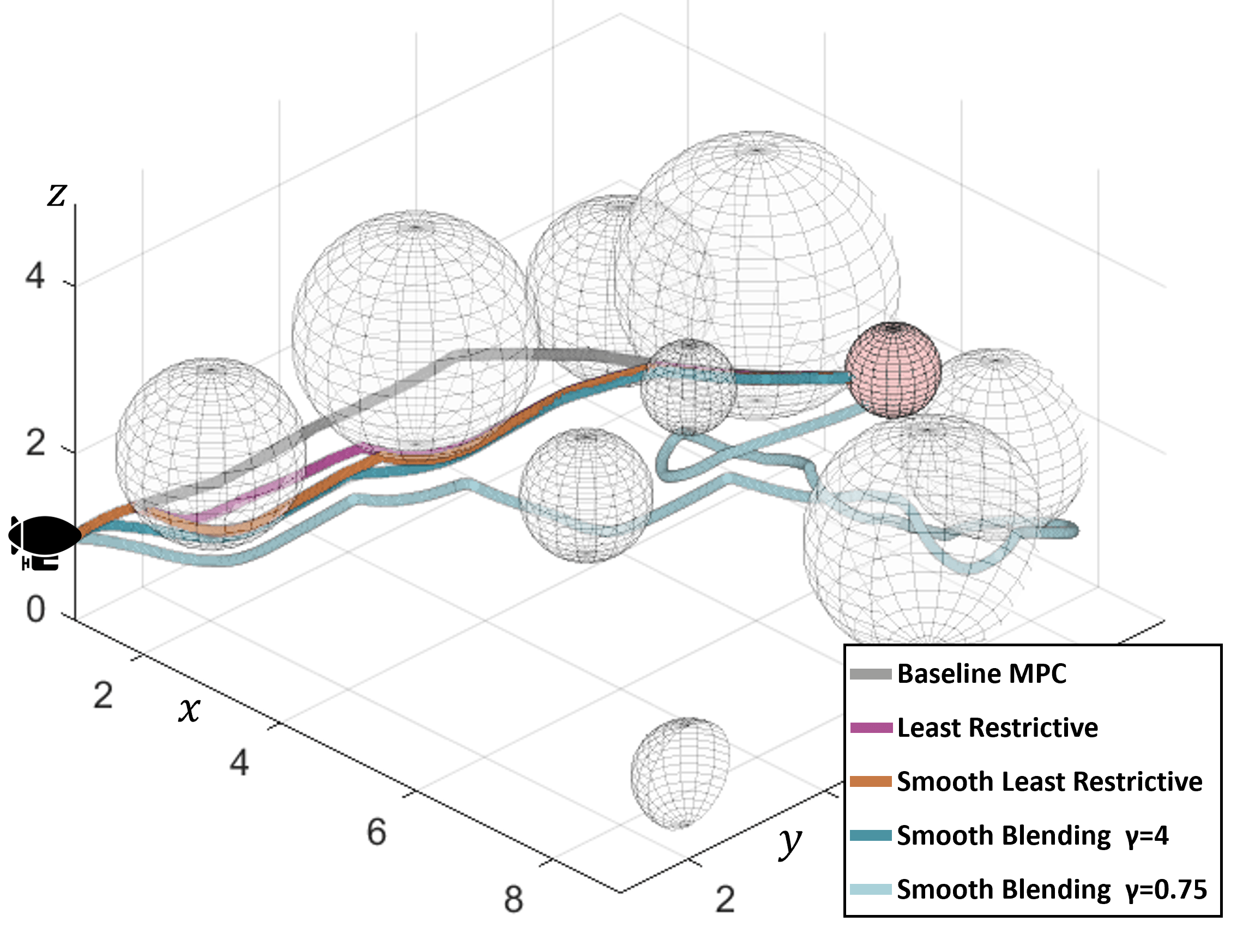
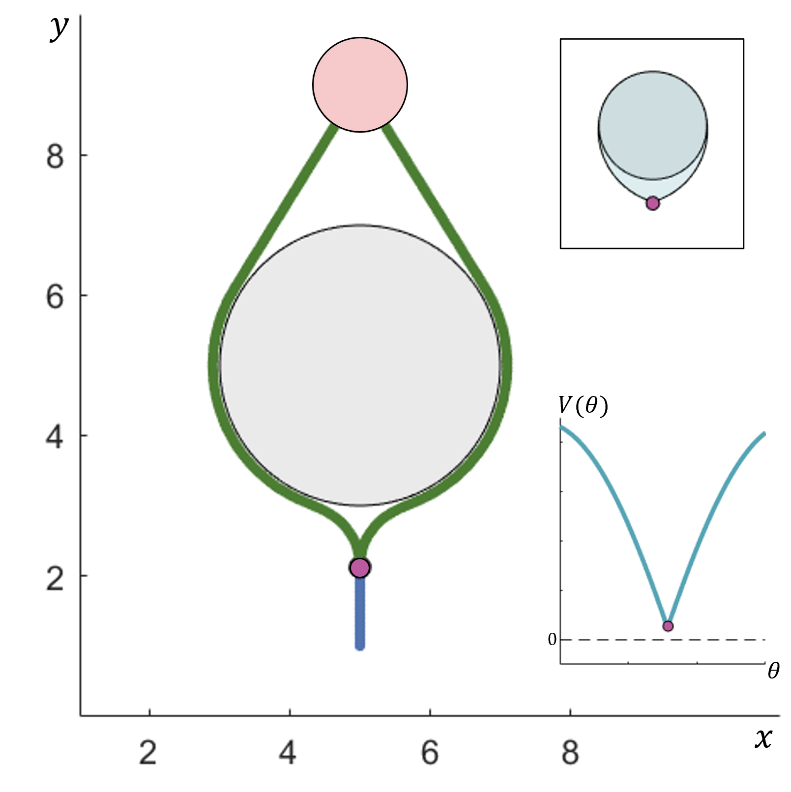
We consider a x x position state space (Fig. 2) where the objective is to reach a target area of radius located at (pink sphere) while avoiding collision with static obstacles represented as spheres of various sizes spread across the position state space. In (3) is the velocity in the plane, the control and disturbance bounds are given as , and .
For this system we use an MPC-based nominal controller, whose objective is to minimize distance between the system and the target area, subjected to the system dynamics and the control bounds. To highlight the impacts of safety filtering, the nominal controller is built such that it does not consider obstacle avoidance in its objective. The system state trajectories and control profiles under the nominal controller are shown in grey in Fig. 7 and Fig. 8 respectively. As expected, the nominal controller fails to satisfy the safety constraint (i.e. avoiding the obstacles).
III Background: Hamilton-Jacobi Reachability
Hamilton-Jacobi (HJ) reachability analysis is a formal verification technique that characterizes the set of states from which the liveness (or safety) constraints can be satisfied with some control under the worst case disturbance. In our work, we will leverage this technique to synthesize liveness (and safety) filters for the nominal controller. In this section, we provide a brief overview of HJ reachability analysis.
III-A Liveness and Safety Problems in HJ Reachability
In HJ reachability analysis, the liveness and safety problems are posed as optimal control problems; informally, both problems intend to find a control signal that steers the system as “deep” into or as “far away” from the target set as possible. To capture this semantic, the minimum distance between the system and the target set over the time horizon is defined as the objective of the optimal control problems. Let be some bounded and Lipschitz continuous function whose sub-zero level is given by the target set: . Here, we present the reachability analysis for the liveness case and then comment on the safety case. Given , the liveness problem is defined in (4):
| (4) |
Where the minimum cost over time for the trajectory is defined as the cost function The above optimization problem (4) finds the minimum distance to the target set over the system trajectory, under the optimal control and the worst case disturbance. Thus, the system can reach the target set if and only if the minimum distance is less than 0, and this minimum distance is captured by the value function:
| (5) |
The value function (5) can be computed using dynamic programming, and it satisfies the following final value Hamilton-Jacobi-Issacs Variational Inequality (HJI-VI) [19, 16]:
| (6) | ||||
Here, and denote the temporal derivative and the spatial gradients of the value function , respectively. The Hamiltonian encodes how the control and disturbance interact with the system dynamics and is given as:
| (7) |
Given the value function, one can also obtain the Backward Reachable Tube of the system. Since is defined to be the set of initial states from which the system can reach the target set within the time horizon despite worst-case disturbance, is the sub-zero level set of the value function:
| (8) |
Consequently, liveness is guaranteed as long as the system state is inside . Conversely, if the system state is outside , the liveness can’t be ensured despite the best control effort. Thus, any live controller must maintain the system state within at all time .
The HJ reachability analysis for the safety problem is similar to that for the liveness problem, except that the control tries to avoid entering . Thus, the role of control and disturbance is switched in (4) and (7). The sub-zero level of the value function gives us the BRT , which represents the set of all states from which the system is guaranteed to enter the target set (the unsafe region in this case), despite the best control effort. Conversely, if the system state is outside the , there exists a controller that will keep the system safe, despite worst-case disturbance.
III-B Default Liveness (Safety) Controller from HJ Reachability
Along with the value function and the BRTs, reachability analysis also provides a liveness/safety controller for the system (referred to as the default liveness/safety reachability controller from here on). At state and time , the default liveness reachability controller is given as:
| (9) |
Similarly, the optimal disturbance is given as:
| (10) |
Intuitively, at any time step, (9) tries to maximally steer the system towards the target set. To understand this, recall that the value function for the livenss problem (4) represents the minimum cost the system can achieve over the time horizon , starting from state and time under worse case disturbance. In the liveness problem, we would like the system to reach a state of lower value. seeks to accomplish this objective by finding a control which steers the system in the direction of greatest decent on the value function (i.e. minimizing the dot product between and the spatial gradient of the value function ). Moreover, it can be shown that as long as the system starts inside , it is guaranteed to eventually reach the target set under despite the worst-case disturbance [4].
On the other hand, the default safety reachability controller’s goal is keeping the system as far away from the target set as possible, and the value function at state is the minimum distance between the system and the target set over the trajectory starting at state under any control signals. Therefore, the optimal safety-preserving control at state should steers system towards a direction that is most aligned with spatial gradients of the value function:
| (11) |
As long as the system starts outside , it is guaranteed to avoid the target set at all times under , despite the worst case disturbance.
Remark 1
The value function often converges for the safety problem, i.e. stops growing after some amount of time, beyond which the system has enough time to maneuver to avoid the target set despite the worst case disturbance. Consequently, we can use the converged value function, which is no longer a function of time , to synthesize safety controllers, and the resulting controllers are time-invariant. In such cases, we can omit the time variable from the controller in (11).
Even though the default reachability controllers respect the liveness/safety constraints, they do not consider other objectives of interests, such as minimizing control energy or tracking some nominal controller. Thus, a natural solution is to blend the default reachability controller with a nominal controller that takes these performance criterion into consideration while respecting safety/liveness constraints, which is the focus of this paper.
Running Example (Liveness). As discussed earlier, in the liveness problem, we are interested in computing , along with associated value function. This requires solving the HJI-VI (6). Traditional methods compute a numerical solution of the HJI-VI over a state space grid [18]; however, these methods suffer from the curse of dimensionality and are not suitable for a 6D system. Instead, we use DeepReach [5] to compute the value function. Rather than solving the HJI-VI over a grid, DeepReach represents the value function as a sinusoidal neural network and learn a parameterized approximation of the value function. Thus, memory and complexity requirements for training scale with the value function complexity rather than the grid resolution. To train the neural network, DeepReach uses self-supervision on the HJI-VI itself. Ultimately, it takes as input a state and time , and it outputs the value , where are the parameters of the NN. We refer interested readers to [5] for further details.
For this system, we use a sinusoidal neural network with three hidden layers, and 512 neurons per layer. The training took approximately two hours for 200 thousand epochs on an NVIDIA RTX 4090 GPU. Using scenario optimization [15], we verify the trained neural network by computing a high confidence error bound over the accuracy of the learned value function. A slice of the obtained BRT projected over the -plane is shown in Fig. 1. As long as the system starts inside the teal region, it is guaranteed to reach the pink region (landing pad) under . The system trajectory under for one such starting state is shown in dark blue in Fig. 1(a) and the corresponding control profiles are shown in Fig. 1(b), (c).
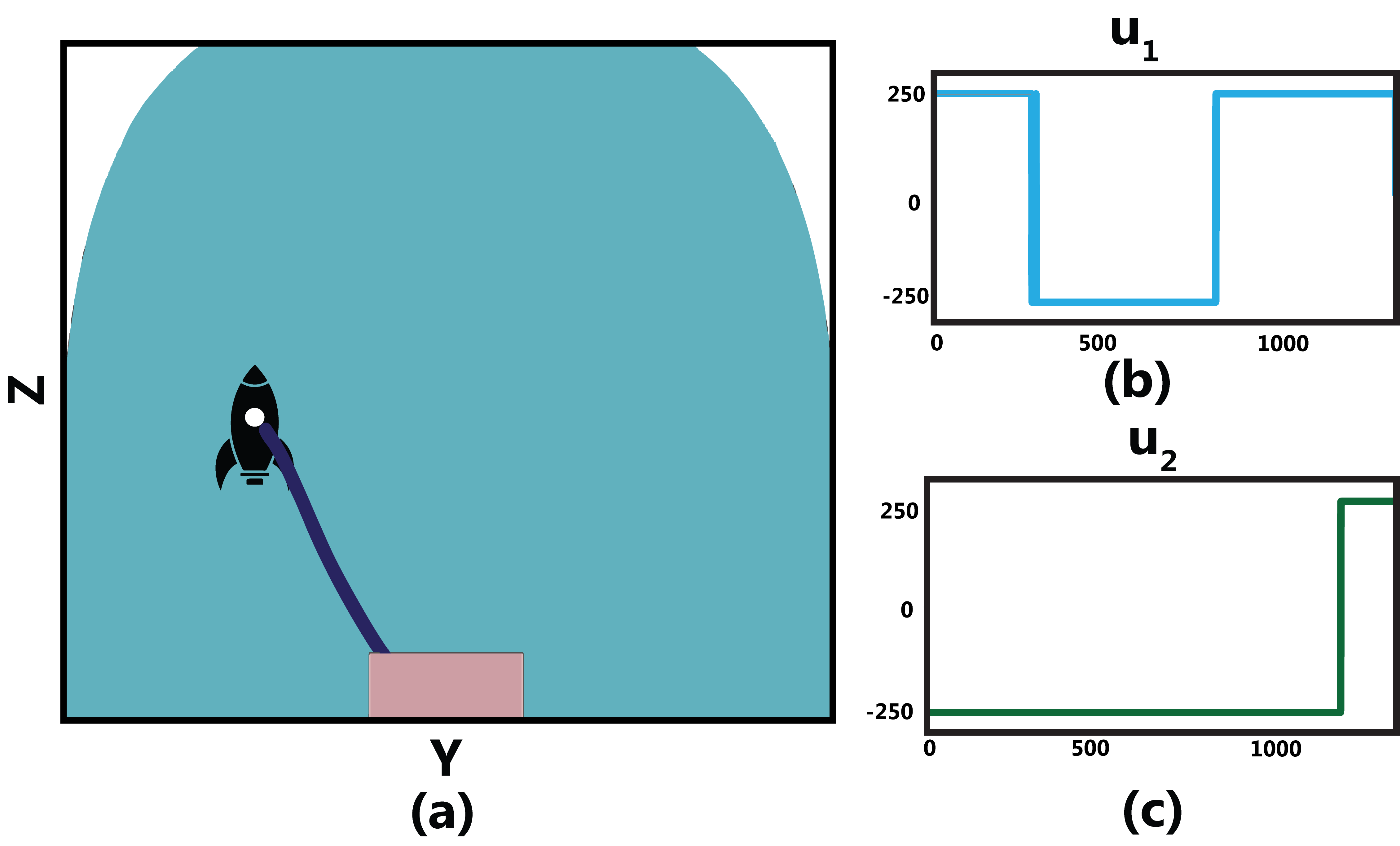
As expected, the rocket eventually reaches the landing pad. However, the default liveness controller only chooses the maximal control authority to steer the system (in this case, ). This is a typical bang-bang nature of the reachability controllers for systems with control-affine dynamics and independently bounded control inputs, that ensures that the value function gradient is always pointing towards the direction of maximum decent.
However, this (a) results in a jittery, high-energy control profile, and (b) does not take into account any performance cost for the controller, which results in a very high total cost for this controller (black bar in Fig. 6).
Running Example (Safety). The safety problem is analogous to the liveness problem, except that the roles of disturbance and control are now reversed, as the control tries to steer the system away from the target set. For this example, we leverage the Level Set Toolbox [20] and its reachability helper library HelperOC [1] to compute a numerical approximation of the BRT. Level-Set methods solve the HJB-VI numerically over a uniformly discretized state space grid. We use a 4D grid of 81 x 81 x 41 x 21 points for our computations. The solution of the HJB-VI provides us with the value function, , which can be used to extract the similar to (8). In this case, the value function converges after 0.5 seconds; thus, we consider the time converged . A 3D slice of for a fixed value of is presented in Fig.2. The expansion of the BRT can be seen in the reverse direction, as states oriented this way will inevitably collide with obstacles if they start too close. By definition of the BRT, as long as the system starts outside the blue region, it is guaranteed to remain safe under the default safety controller (11).
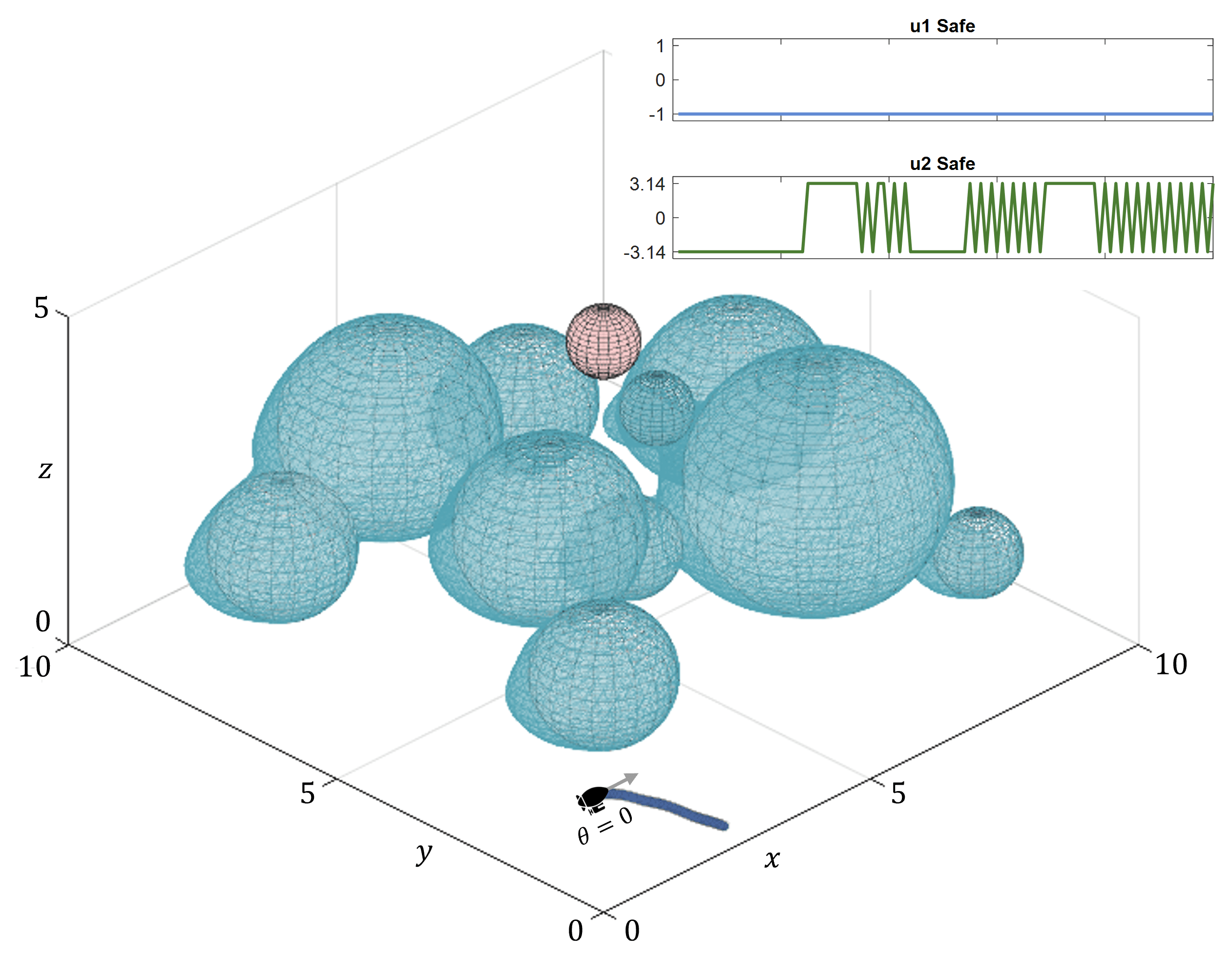
The system trajectory under starting at a state outside the BRT and the corresponding control profiles are shown in Fig. 2. Once again, the system remains safe under the default safety controller as expected; however, the default safety controller steers the system as far away from the obstacles as possible, disregarding any other performance criterion the system might have (such as reaching the pink goal region in this case). Moreover, the control profile is jittery, which is typically undesirable for real-world applications.
IV Liveness Filtering Using HJ Reachability
The default controller obtained from the reachability analysis ensures liveness, but it does not consider other performance objectives. In this section, we first use reachability analysis to characterize the set of all liveness-ensuring control inputs at a particular state. We then use this set to design different liveness filters.
IV-A Characterizing the set of live controls
At state and time , the set of all liveness-ensuring control inputs (abbreviated as live controls for the remainder of the paper) is given as:
| (12) |
Here, is the optimal disturbance given by (10). Intuitively, (IV-A) is the set of all controls that instantaneously keep the next state of the system inside (or at the boundary of) , despite the worst case disturbance . This ensures that the system can still reach the target set from the next state, thereby ensuring liveness recursively.
We will next use (IV-A) to characterize . We assume that ; otherwise, the system state is already within the target set and no further control action is needed.
Lemma 1
Assume that the value function is differentiable for all and . Let be any state such that . Then the set of live controls at is given as:
| (13) |
The proof of Lemma 1 is in the Appendix. Intuitively, (13) states that is the set of all admissible controls when the system state is in the interior of . This makes sense as the system can apply any control and instantaneously remain inside for a sufficiently small time step. On the other hand, when the system state is outside , liveness can’t be ensured despite the best control effort, resulting in an empty set. Finally, when the system state is at the boundary of , is given by the controls that ensure the total derivative of the value function, , to be 0 (i.e., the control inputs that keep the system state instantaneously at the boundary of ).
There are a few interesting observations to be made about the set of live controls in (13):
-
1.
Lemma 1 provides a time-dependent characterization of the live control inputs, allowing us to capture time-constrained liveness properties (e.g., reach the target set within seconds), as opposed to just asymptotic liveness.
-
2.
For control and disturbance-affine system dynamics, the condition of is linear in . To see this, suppose the system dynamics are given by . Its total derivative is given by:
We can observe that is now a linear equation of , where and . Thus, is given by a hyperplane in (a point if the control space is one-dimensional), whenever the system state is at the boundary of . As we will see later, this will make the liveness filter design particularly computationally efficient for control-affine systems.
-
3.
Control inputs given by the default liveness controller (9) is always contained within . The following corollary formalizes this result.
Corollary 1
.
Thus, the default controller can be used to steer the system to the target set, consistent with our expectation.
The real utility of (13) is that it can potentially provide more than one liveness-ensuring control inputs, whereas the default liveness controller can only provide one at a given state and time . We now formally establish that applying any control inputs from is sufficient to ensure that the system eventually reaches the target set within in the time horizon .
Lemma 2
Suppose the system starts inside at state at time . If the system applies control , then such that .
Lemma 2 effectively allows us to use any subset of for the projection of the nominal controller, while still maintaining liveness. This suggests the following general structure for liveness filters:
General Liveness Filter. Given a nominal controller, , a general liveness filter can be formulated as:
| (14) |
In (14), we refer to as the projection operator and as the projection set. Since , the above filter makes sure that , thereby ensuring system liveness at all times (by Lemma 2). Nevertheless, different choices of and will lead to different trade-offs between performance and liveness.
To make sure that the optimization problem (14) can be solved in a computationally efficient manner, it is often desirable to use a projection operator and set that are convex in for a given and . A particularly popular choice in the literature for is the distance from the nominal controller, i.e., . For the remainder of this section, we use this projection operator and choose three different that result in particularly interesting liveness filters. We will conclude the section by comparing the resultant filters.
IV-B Least Restrictive Filter
To blend performance with liveness, the reachability analysis is typically applied in a least-restrictive fashion [4]:
| (15) |
The least restrictive (LR) filter follows the nominal controller when the system state is in the interior of (i.e. ), and it takes corrective actions given by when the system is on the boundary of or at the risk of exiting . This ensures that the system never exits . The controller in (15) is least restrictive in the sense that it follows the given nominal controller that can optimize criteria besides liveness, and only interferes when the system is at the risk of breaching liveness. Consequently, the system can optimize other objectives while progressing towards the goal, but such freedom is not afforded by as its sole objective is to ensure system’s liveness.
The LR filter (15) can be obtained using our general framework (14) by using the following :
| (16) |
Thus, is the set of all permissible controls whenever the system state is inside and is given by a singleton when it is at the BRT boundary. It is easy to verify that for all and . Thus, the system will always remain live under the LR filter.
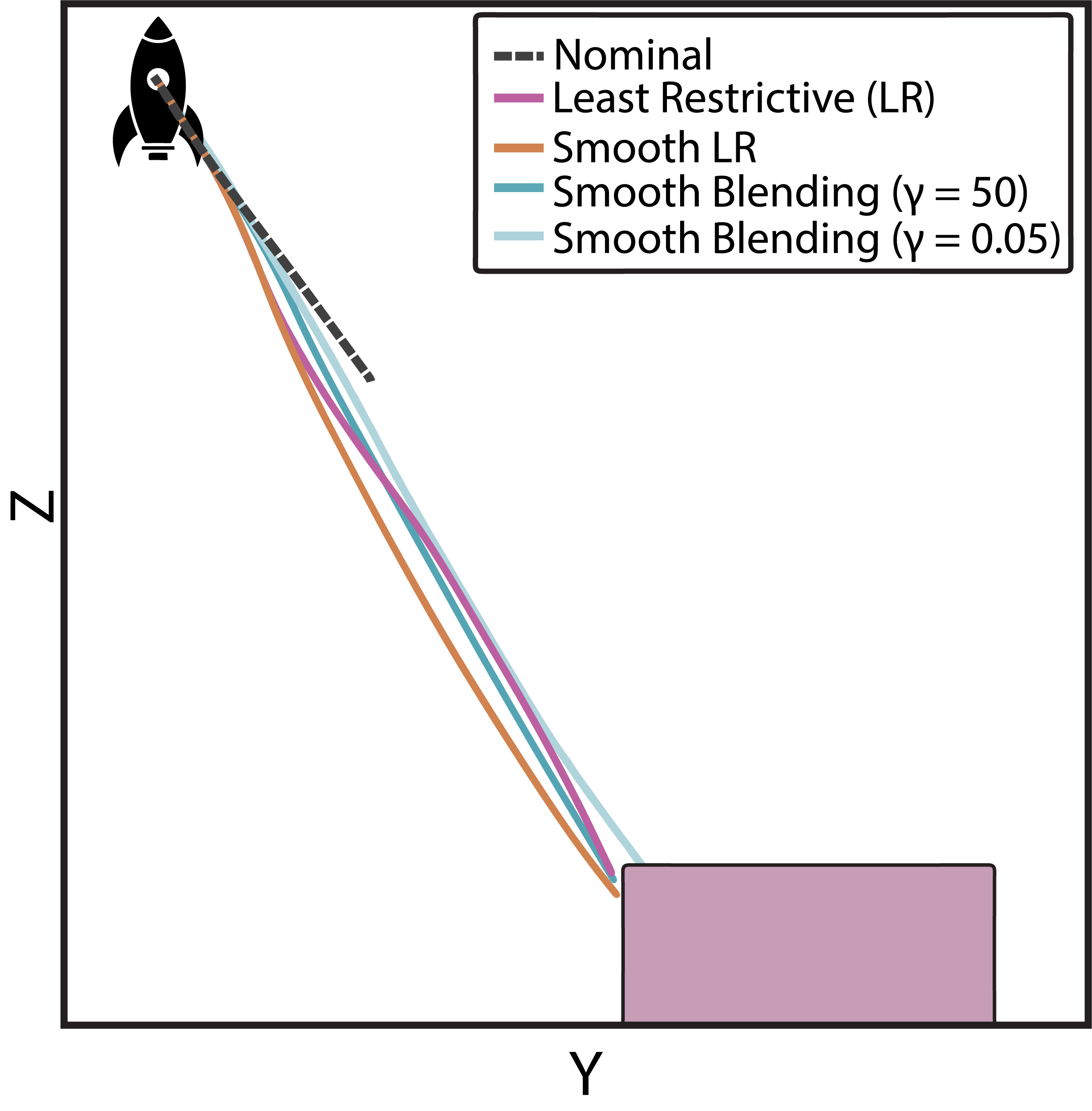
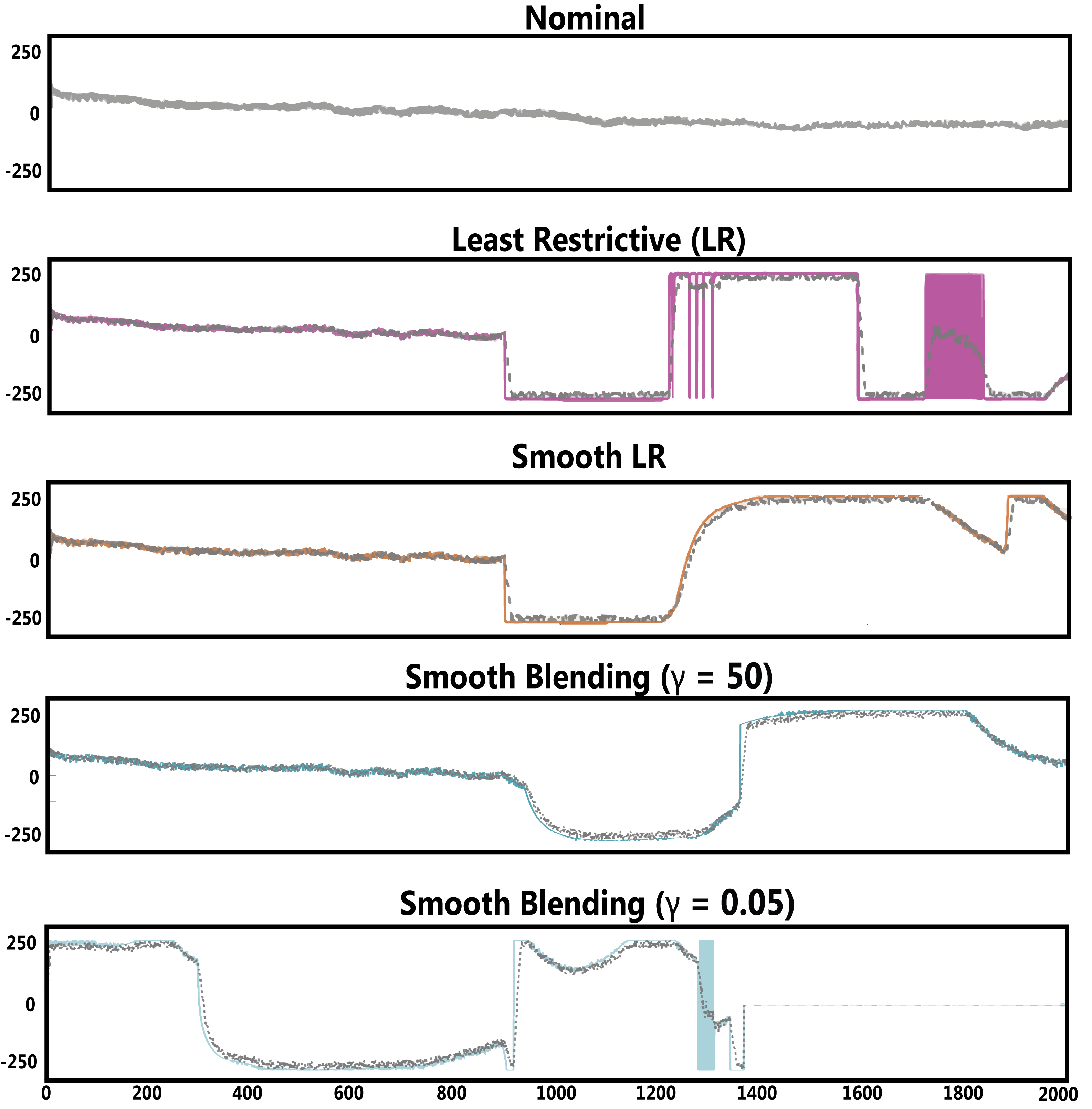
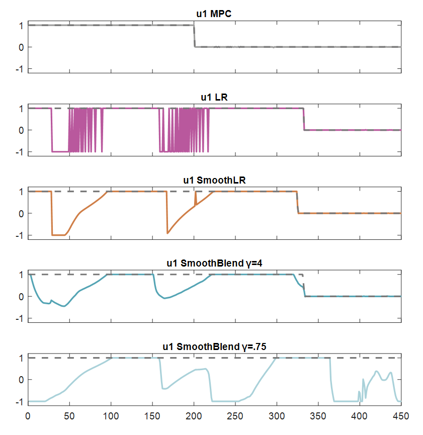
Running Example (Liveness). We now demonstrate the LR filter (15) on the running example. The corresponding system trajectory and the control profile (for ) are shown in purple in Fig. 3 and 4, respectively. As expected, the LR filter chooses between and to steer the system towards the target set. However, as discussed earlier, using results in bang-bang behavior (as evident from the spikes in the control profile) and high control energy (purple bar in Fig. 6). In the next subsection, we propose a smoother version of the LR filter to overcome this challenge.
Remark 2
Upon careful observation, one might note that the LR filter does not take the system fully inside the target set within the time horizon (the purple trajectory is slightly outside the target set in Fig. 3). This discrepancy between theory and practice is due to the effect of using a discrete-time simulation of a continuous-time system, which sometimes causes a slight delay in the switching between the nominal and the default controller. We will discuss this aspect more as well as a few potential solutions in Sec. VII.
IV-C Smooth Least Restrictive Filter
While the LR filter (15) blends performance and liveness, it still switches abruptly to at the boundary of , leading to a high energy, bang-bang behavior near the boundary of . To overcome this challenge, we propose an alternative liveness filter that uses the full control authority available to the system as the projection set, rather than just :
| (17) |
i.e., for all . Intuitively, the above optimization problem computes a control input at each time instant that is “closest” to the nominal controller, yet is within the set of live controls. Furthermore, since whenever , we can simplify the filter in (17) as:
| (18) |
where is obtained by solving the following optimization problem:
| (19) |
where is the optimal disturbance given by (10). We refer to the controller in (18) as the smooth least restrictive (smooth LR) filter. Similar to the LR filter (15), the smooth LR filter (18) follows when the system state is in the interior of . However, when the system state is at the boundary of , rather than using , it chooses a live control that is closest to the nominal control by solving a Quadratic Program (QP), thus allowing for a smoother control profile.
Remark 3
Running Example (Liveness). The trajectory and control profile corresponding to the smooth LR filter are shown in orange in Fig. 3 and 4. We observe that the smooth LR filter effectively “smoothes” out the bang-bang behaviors that the LR filter displayed; control profile now follows a gradual curve dictated by the QP formulation. This results in lower control energy (orange bar in Fig. 6) and less jittery behavior of the resulting system when compared to the original LR controller.
IV-D Smooth Blending of Performance and Liveness
The LR and smooth LR filters employ live controls as a last-minute resort when the system is at the risk of breaching liveness. Despite its simplicity, this sudden and inconsistent switching to a liveness controller has a few drawbacks: (a) switching at the BRT boundary can still result in a jittery control profile if the nominal control is far from the set of live controls; (b) a last-minute switching can lead to liveness violation upon the slightest delay in switching. To remedy these drawbacks, we take inspiration from the CBF literature. Specifically, we introduce a “CBF-like” constraint to define the projection set that encourages the filtered control to be “more” liveness-ensuring as the system approaches the boundary of :
| (20) |
The left hand side of the constraint in (20) is the total derivative of evaluated at state and time . Thus, intuitively, the above constraint limits the rate at which the value function can increase, i.e., approach the boundary of , even when the system is farther from the boundary of . When the system is at the boundary of the , the RHS is zero and the controller must output a control that would keep the system at the same value. Specifically comparing with the LR and smooth LR filters in this section, the projection set in (20) blends with in such a way that the system can take gradually more stringent corrective actions as the system becomes more at risk of breaching the liveness, resulting in less jerky controls.
The behavior of the control constraint in (20) is quite similar to that of the CBF constraint in CBF-QP [3], as determines how quickly the value function can change. However, it can be difficult to find a valid CBF function in the presence of control bounds and disturbances, requiring online tuning of to make sure that the constraint remains feasible at all times, which can be quite challenging in practice. On the other hand, the reachability-based controller in (20) is always live and feasible, as we prove next, bypassing the need of tuning to ensure liveness.
Lemma 3
Let be any state such that and . Define . Then (a) is non-empty, and (b) for all .
Intuitively, Lemma 3 states that (a) using the projection set in (20) always results in a feasible filtering problem, and (b) liveness is always guaranteed under the resultant control input, regardless of the value of . An alternative interpretation of Lemma 3 is that, as long as the value function is differentiable, it acts as a robust CBF for any value of and can be used to synthesize CBF-like controllers. Even though a number of works have synthesized CBFs using the reachability analysis (e.g., [9]), these methods need to explicitly select a value of during the value function computation, making it challenging to tune online. In contrast, Lemma 3 indicates that can in fact be chosen online, independent of the value function computation.
Nevertheless, the value of still affects the blending of and . Specifically, as , the constraint in (20) no longer limits the rate of change in the value function and the blending controller starts behaving like the smooth LR filter (18). Thus, the system prioritizes the performance until the liveness is at risk. On the other hand, as , the constraint in (20) becomes very stringent and does not allow value function to increase. Consequently, the blending controller starts behaving like the default liveness controller in (9), prioritizing the system liveness over performance. Thus, by choosing in between the two extremes, we are effectively blending these two controllers, creating different trade-offs between liveness and performance.
Running Example (Liveness). We show the smooth blending filter for different values of . The trajectories are shown in different shades of cyan in Fig. 3. In the first case with , the system’s behavior is very similar to the default reachability controller, where the system is very cautious and avoid moving towards the BRT boundary. However, from the corresponding control profile in Fig. 4, we notice that the controller follows a slightly smoother version of the bang-bang behavior that we saw in Fig. 1 and the control applied is not always the maximal control, especially towards the later times. On the other hand, using , the system goes very close to the boundary of the BRT, behaving similarly to the smooth LR filter, as expected.
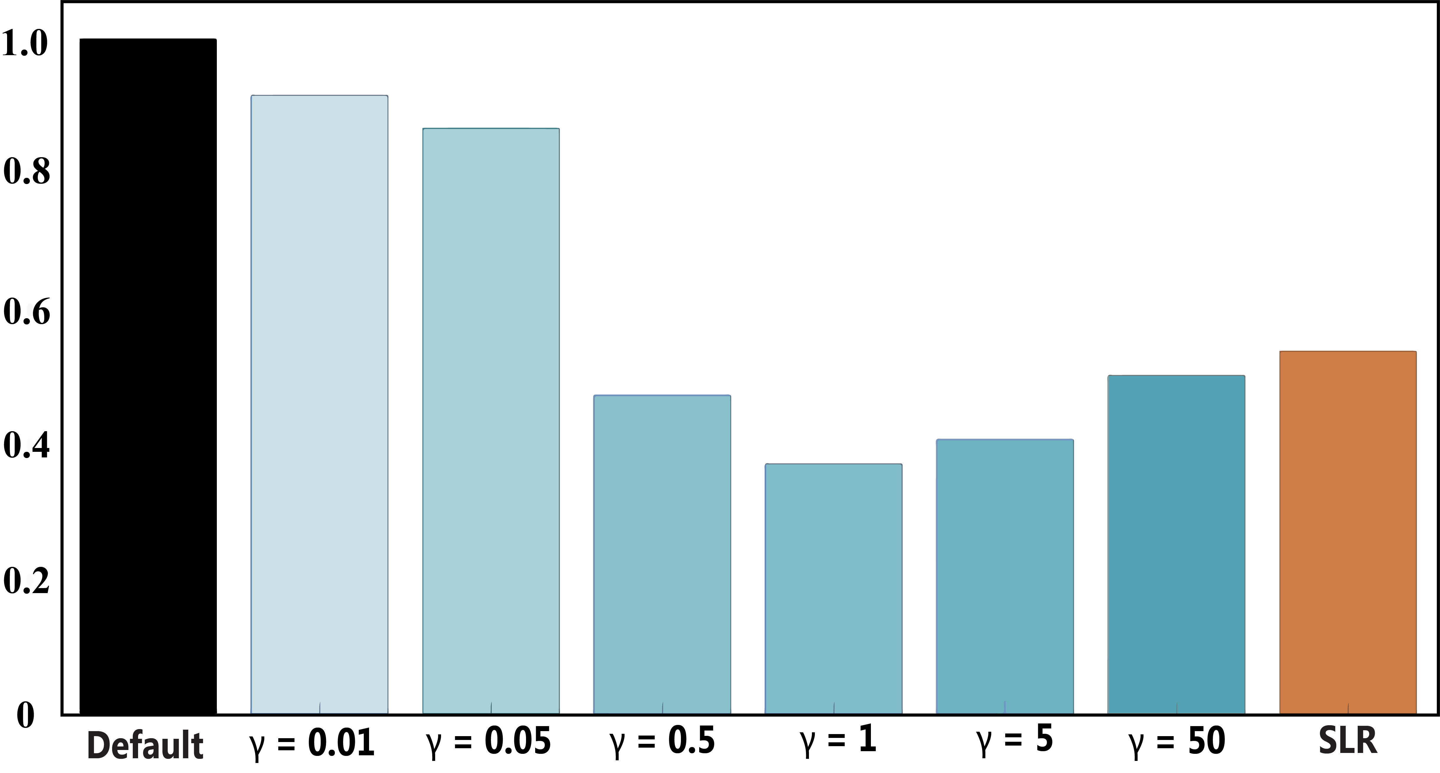
Effect of . To illustrate the effect of , we plot the overall (normalized) trajectory cost for different values of in Fig. 5. As evident from the figure, the choice of can significantly affect the performance of the smooth blending filter. Specifically, as approaches , the system behaves more and more like , keeping stringent liveness characteristics. This liveness, however, comes at the cost of a drop in performance (the controller cost is very high for small ). On the other hand, as we increase (till around ), we see a proclivity towards using a controller That is close to the nominal controller while encouraging liveness. This results in a significant decrease in the trajectory cost. However, beyond a certain ( in this case), the cost is again seen to rise slightly. This is because, for such a high , the controller is allowed to behave more and more like the smooth LR filter. The blending filter chooses the nominal controller as long as the system remains live; however, this choice leads the system closer to the BRT boundary, and the controller has to revert to a high-cost control in order to keep the system live, ultimately raising the overall controller cost. Hence, for high , the smooth-blending controller have a similar cost as the smooth LR controller.
IV-E Comparison of Different Liveness Filters
We now compare the performance of different liveness filters across five metrics:
-
1.
minimum distance to the target set, measuring the liveness of each filter;
-
2.
total cost accumulated over the trajectory, measuring the performance of each filter;
-
3.
controller computation time per step, measuring the filter latency;
-
4.
control energy, measuring how much control authority is used;
-
5.
jerk energy in control, measuring the jerk in the control profile.
The obtained results are summarized in fig. 6.
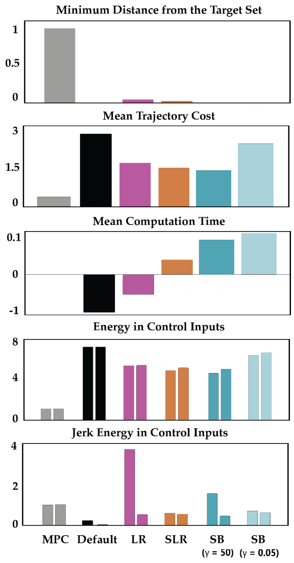
First of all, we note that despite a poor nominal controller, all liveness filters steer the system very close to the target set (minimum distance to the target set is close to zero). However, the LR filters have a small non-zero distance to the target set. This is because in our simulation we use a small but non-zero timestep, which causes a small delay in the switching from the nominal to the liveness ensuring controller at the BRT boundary, resulting in the system state being outside of the BRT momentarily. We discuss this aspect further, as well as potential remedies in Sec. VII-A. Interestingly, we note that even though for high , we expect the smooth blending filter to behave similar to the smooth LR filter, we do not observe a similar loss of liveness in the smooth LR filter. This is because even for a high , the smooth blending filter applies the liveness controller before the system reaches the BRT boundary.
In terms of performance, we note that results in a very high trajectory cost, which in our running example is dominated by a high control energy cost due to its bang-bang nature. In contrast, liveness filters balance liveness with performance, resulting in a lower trajectory cost. In this case, we note that smoother the control profile, the lower the trajectory cost, resulting in a better performance by smooth blending filter followed by smooth LR filter followed by LR filter. We further note that for , the performance of the smooth blending and smooth LR filters is very close, as expected. However, as decreases, the smooth blending filter prioritizes liveness over performance, resulting in an increased trajectory cost. We see a very similar pattern in the control energy plots.
Next, we compare the computation time of different controllers, normalized by the mean computation time for the . Here, emerges as the controller of choice, as it only requires computing , which in typically is very fast, especially when the value function is represented as a neural network. In fact, in this case, computing the nominal controller is more expensive than computing , which is why the mean computation time for the default controller is negative. For the same reason, the LR filter also leads to a negative computation cost, as it resorts to when the system state is at the BRT boundary. Compared to the aforementioned controllers, the smooth LR and smooth blending filters leads to a substantially higher computation time, as they require solving an optimization problem to compute the control input which constitutes most of their computation time. Moreover, the smooth LR filter has a much lower computation cost among the two because it only solves an optimization problem when the system state is at the BRT boundary. In general, the better the nominal controller is at maintaining liveness, the smaller the computation time for the smooth LR filter.
Finally, we measure the average jerk in the control trajectories generated by different filters. Despite its extremum seeking behavior, the default controller in this case has a low jerk, as the controller does not switch between the two extremes often. In contrast, the LR filter leads to a sudden switch from the nominal controller to at the BRT boundary, leading to a chattering and high jerk. The smooth LR and smooth blending filters smooth out these transitions between the two controllers, leading to lower jerks.
Overall recommendation. Upon comparing different liveness filters, we recommend to use the smooth blending controller with a high value of , as it nicely tradeoff performance and liveness, while maintaining a low jerk. At the same time, using a very high can spare the user from tuning of , which can significantly affect the performance of the system (Fig. 5). A close second choice is the smooth least restrictive filter, which also share the above advantages. In addition, it has a lower computation latency, making it particularly suitable for real-world robotic systems. One disadvantage of the smooth LR filter is that it can result in a loss of liveness if not implemented with a small enough timestep, which is a key reason behind our overall pick.
V Safety Filtering Using Reachability Analysis
We now turn our attention to safety filtering. Similar to liveness filtering, we will first characterize the set of all safe control inputs for the system, and then use it to design various safety filters. As noted in Remark 1, we will use the converged value function for designing safety filters. Nevertheless, the proposed filters can easily be extended to incorporate time, similar to liveness filters.
V-A Characterizing the set of safe controls
To ensure safety, we would like the system to stay out of the at all times. Thus, intuitively, the set of safe control at a state are the control inputs that instantaneously keep the system state outside , thereby ensuring recursive safety. Mathematically,
| (21) |
The proof of (21) follows similarly to that for the liveness case, except that we do not need to account for the time-derivative of the value function in the controller expression, since the value function has converged. The set of safe controls is , when the system state is outside . When the system state is at the boundary of , the set of safe controls are those that keep the state instantaneously at the boundary of . Finally, safety cannot be ensured under any control input if the system state is inside . An explicit characterization of suggests the following general structure of a safety filter:
General Safety Filter. Given a nominal controller, , a safety filter can be constructed as:
| (22) |
Similar to liveness filters, we refer to as the projection operator and as the projection set. Since , the above filter makes sure that the system remains safe at all times.
V-B Least Restrictive Safety Filter
The set of safe controls can be used to design a least restrictive safety controller for the system:
| (23) |
Similar to the liveness case, the least restrictive safety controller follows the nominal controller when the system is not risk of breaching safety, and it switches to (11) when the system is on the boundary of the BRT. The LR safety filter in (23) can be obtained using our general framework in (22) by using the following :
| (24) |
Running Example (Safety). We next demonstrate the least restrictive safety filter on our running example. The corresponding system trajectory and control profiles (for ) are shown in Fig. 7 (purple) and Fig. 8 respectively. Applying the LR filter on top of the baseline MPC controller allows the system to avoid collision with obstacles, but it comes with the shortcoming of an overly aggressive control profile at the boundary of the unsafe set near the obstacles, as the controller switching and the bang-bang nature of results in a jittery control profile that jumps to the limits of the control authority.
V-C Smooth Least Restrictive Safety Filter
Some of the shortcomings of the least restrictive filter can be addressed by the smooth least restrictive filter:
| (25) |
where is obtained by solving the following optimization problem:
| (26) |
The smooth least restrictive filter can readily be obtained using our general filtering framework by selecting , i.e., using the maximal safe control set at all times.
Compared to the least restrictive filter, the smooth least restrictive filter allows the system to take a control action that is “closest” to the nominal control, yet keeping it safe at all times, leading to a smoother control profile. Note that we have dropped the term from the constraint in (26) because we assume the value function has converged.
Running Example (Safety). The results of applying a smooth least restrictive filter to the running example is shown in orange in Fig. 7 and its control profiles in Fig. 8. Wherever possible, the controller avoids the bang-bang nature of by allowing the selection of controls that are close to the nominal controller, yet guaranteed to be safe. This smooths out an overly aggressive control profile generated by the least restrictive filter at the boundary of .
V-D Smooth Blending of Performance and Safety
Again quite similar to its liveness counterpart, the smooth blending safety filter utilizes the CBF-like constraint to blend the safety and performance objectives.
| (27) |
Similar to the least restrictive and smooth least restrictive filters, the smooth blending filter allows the system state to move towards the boundary of (i.e., the value function can decrease), but unlike the aforementioned controllers, it limits the rate (determined by the user-defined coefficient and the value of the current state ) at which the value function is allowed to decrease. This phenomenon (a) avoids a sudden switching to , leading to a smoother profile; and, (b) encourages the system to maintain a non-zero distance from the BRT boundary at all times.
The smooth blending filter can be obtained by using within the proposed general safety filter framework. Similar to Lemma 3, it can be shown that for all .
Running Example (Safety). Resulting state trajectories of applying the smooth blending filter for two different values of are shown in blue and light blue in Fig. 7, and their control profiles are shown in Fig. 8. As evident from the control profiles, the smooth blending controllers do not produce any sudden switching since they are free to select controls closer to the nominal controls as long as the decrease in value is bounded by the prescribed rate. This rate is adjusted through the parameter , which determines how “confident” the system feels moving toward the unsafe states at a given value level. For this example we used values of and . A larger value of allows the system trajectory to move closer to the obstacles (increasingly behaving like a smooth LR filter), while a smaller value results in a more conservative behavior (behaving similar to the default safety controller). This can also be seen from the system trajectory corresponding to , wherein the safety filter is pushing the system away from the obstacles to ensure that the value function doesn’t decrease too much (similar to the default safety controller), resulting in a very curvy and inefficient trajectory to the goal. In contrast, the trajectory corresponding to ventures fairly close to the BRT boundary. These trajectories highlight a critical characteristic of smooth blending filter – the system performance can heavily depend on . Thus, a proper tuning of might be needed to obtain a satisfactory behavior.
V-E Comparison of Different Controllers
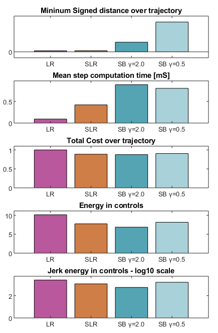
In this section, we present a comparison between the proposed filtering schemes across five metrics: total cost accumulated over the trajectory, minimum distance to the obstacle set, the controller computation time per step, control energy, and control jerk energy. The control profiles for are shown in Fig. 8 and the metrics for both and are presented in Fig. 9.
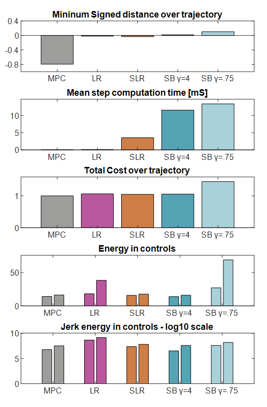
The baseline MPC controller does not consider any obstacles, thus getting the most negative signed distance as it penetrates through them; for all other metrics, it will be considered as the base case we will use for comparison.
The least restrictive filter maintains safety and only gets minimum penetration over obstacles; this slight penetration is due to the switching happening not strictly at but when the value function is negative due to finite grid and time step resolution. The safety enforcement increases the total cost over the trajectory compared to the base MPC controller, because when safety is at risk, it steers the system away from unsafe states which conflicts with the baseline controller objective. The least restrictive filter is the fastest to implement among all safety filters as the default safety controller can be computed quickly using the BRT, without requiring to solve any optimization problem, unlike other safety filters. The downside lies in high energy and high jerk in the controls due to the bang-bang nature of the default safety controller.
The smooth least restrictive filter also suffers from some penetration over obstacles because it uses the same switching condition as the regular least restrictive filter but presents improvements both in the energy and jerk of the controls as it no longer relies on purely bang-bang safety controller, with the drawback of increased computation time per step as (26) needs to be solved each time that safety is at risk.
The final two controllers correspond to smooth blending of performance and safety for two values. Inclusion of in the safety filter allows the system to reason about safety before reaching the boundary of the unsafe set, allowing the system to maintain a positive signed distance to obstacles over the whole trajectory. This comes at the expense of an increased mean calculation time, especially for the case with smaller as the more conservative constraint in (27) is slightly harder to solve. It is also worth noting that a high behaves quite similarly to the smooth LR filter, without its downside of accidentally penetrating the obstacle due to a last-minute switching.
Overall recommendation. Similar to the liveness case, we overall recommend to use the smooth blending safety filter with a high value of , as it nicely tradeoff performance and safety, while maintaining a low jerk. At the same time, using a very high can bypass the need for tuning of .
VI Hardware Experiments
We next apply the proposed safety filters on a Turtlebot 4, a Dubins-like robotic platform (see Fig. 10). The robot needs to reach a goal position in an area situated with multiple obstacles. To complete this task, we use a shooting-based MPC nominal controller that does not consider obstacle avoidance in its objective. We choose this nominal controller on purpose to highlight the effect of safety filtering. The nominal controller will be filtered using the techniques presented in Section V to guarantee safety while navigating towards the goal.
We model the dynamics of the system as a Dubins car with and where the state represents the and positions and the heading of the robot:
| (28) |
The BRT for this experiment is calculated on a grid of points, which gives a resolution of in position over the experiment space and in orientation. The BRT was computed until convergence (in this case, the BRT converges after a horizon of ). The converged value function is then used to synthesize various safety filters.
We assume perfect state measurement during our experiments. The system state is obtained through the robot’s internal pose estimation capability given by a combination of measurements from an IMU, optical floor tracking sensor, and wheel encoders. To avoid accidental breach of safety in least restrictive and smooth least restrictive filters due to limited grid resolution and discrete timestep (see Sec. V-B), we use a non-zero threshold to activate the safety controller. Specifically, we use the condition (instead of ) to trigger switching to . A value of was used in the experimental results shown.
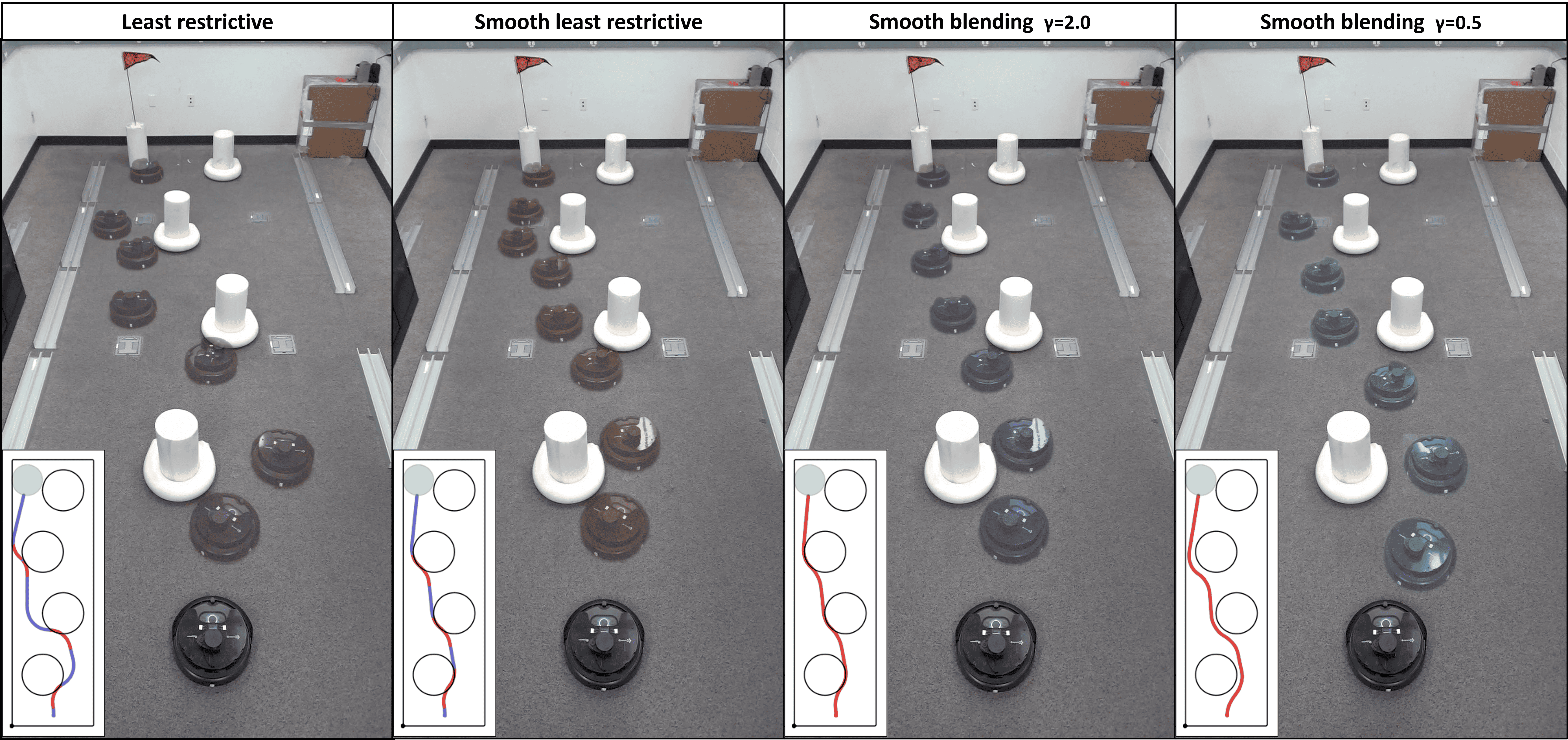
The robot trajectories corresponding to different safety filters are shown in Fig. 10. The corresponding control trajectories are shown in Fig.11. We also compare different safety filters across various metrics. These results are shown in Fig. 10 (right).

With this information, we highlight the core characteristics of each safety filter:
Least Restrictive Filter: Even though the least restrictive filter keeps the system safe with fast queries of the default safety controller, the bang-bang nature of the safety controller forces the system to take sharp turns. Additionally, it results in high energy control inputs. Together, these results in a high accumulated cost over the robot trajectory.
Smooth Least Restrictive Filter: Similarly to the previously presented simulation results, this method shows improvements compared to the least restrictive filter, both in the total energy and jerk of the control profile. It also keeps lower accumulated cost as the safe control is trying to align with the underlying nominal controller. The drawback comes in the form of an increased computation time per step, as (26) must be solved each time the system safety is at risk. It is also worth noting that using a non-zero threshold to active the QP-based safety controller in (25) avoids any accidental collision with the obstacles, unlike our simulation results.
Smooth Blending of Performance and Safety: The final two trajectories show filtering with the smooth blending filter with and . The use of the filter on every time step of the trajectory (rather than just at the BRT boundary) allows the system to stay further away from the obstacles. The drawback is the requirement to solve (27) on each step, which results in an increase in the mean step computation time. The computation time, however, is still low enough to have any significant impact on robot operation. We also observe that a smaller value of leads to a more cautious robot behavior, reflected in the largest separation to obstacles among all safety filters (see Fig. 10). This comes at the cost of an increased control energy, control jerk, and an overall higher accumulated cost, as compared to .
VII Practical Considerations
VII-A Effect of a finite simulation timestep
The filters designed in this paper are based on the assumption that the control input can be applied to the system in a continuous time fashion. However, controller implementation on a real system often involves a zero-order hold, leading to a non-zero simulation timestep . If is too large, the proposed controllers may no longer be able to ensure liveness/safety for the underlying continuous time system. For example, an least restrictive filter ensures liveness by switching to at the boundary of the BRT. However, under a finite , may no longer be able to keep the system state within the BRT, as the liveness is only guaranteed under a continuous time, state feedback reachability controller. This discrepancy between the continuous-discrete structure is demonstrated in Fig. 12, where we show the trajectory variations generated by the least restrictive filter for different values of .
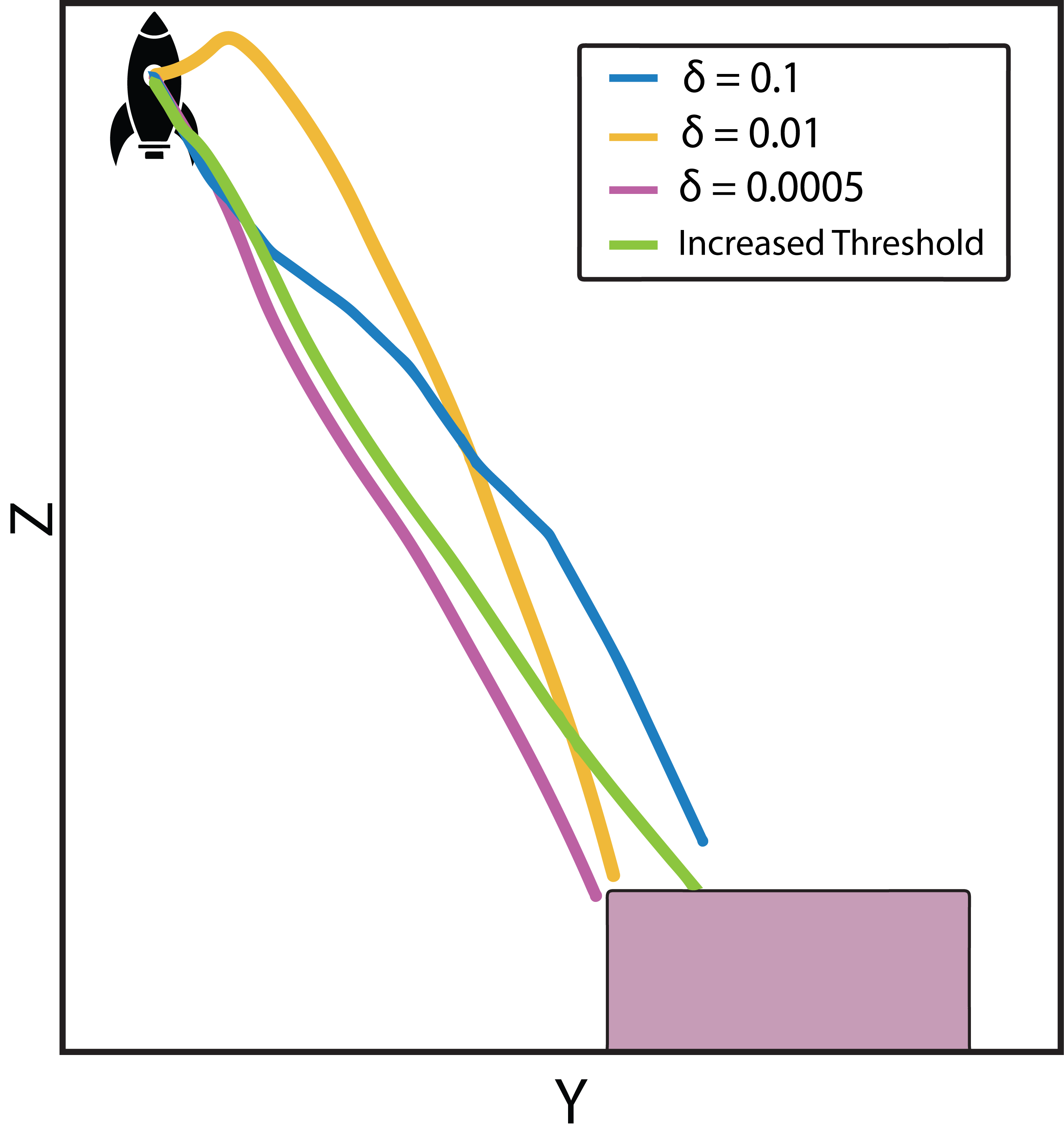
Such effects are more pronounced in the least restrictive filters since there, the system evolves along the BRT boundary. If our simulation timestep is too high, it is highly possible that our system temporarily escape the BRT and enter the unsafe region. One possible solution could be a faster feedback with gradually decreasing as the system approaches the BRT or adaptive depending on the value function. One can also use a discrete-time variant of the BRT computation itself. Alternatively, instead of the switching at the BRT boundary () as seen in Eqn. (23), we can choose to switch with some margin from the boundary. This slightly modifies the least restrictive controller as follows,
| (29) |
An example corresponding to is shown with the green line in Fig. 12. As evident from the figure, this strategy is able to maintain liveness at all times and eventually reaches the target set (unlike the pink trajectory using the same , but ). This strategy was also employed during our hardware experiments to avoid accidental collisions with the obstacles. Finally, one can use smooth blending filter with a high value of to avoid liveness/safety loss at the BRT boundary. Nevertheless, a thorough analysis of effect of a finite simulation timstep on system liveness/safety would be a promising future research direction.
VII-B Non-differentiable value functions
The proposed controllers in this paper rely on differentiability of the value function, which may not always be the case [12, 19]. To discuss the impact of non-differentiability of the value function on the proposed controllers, consider the Dubins car dynamics in (28). Moreover, we consider the smooth least restrictive safety filter for our illustration. This requires solving an optimization problem where we find the closest control to the nominal control, such that the condition with is met.
The goal region and the obstacle are shown in light pink and gray respectively in Fig. 13. The nominal planner, unaware of the environment obstacle, plans a straight path to the goal region (blue trajectory).
Correspondingly, the safety controller engages when the system state reaches the BRT boundary (obstacle and BRT shown in top right inlet and boundary point in purple). The value function has a kink at this state, wherein the system has two equally viable option (hard left-turn or hard right-turn) to barely avoid the obstacle. However, at this state, the value function gradient in the theta direction does not exist, as is evident from the bottom right inlet in Fig. 13.
Thus, one can no longer use the safety filters that rely on the value function gradient (such as a smooth least restrictive filter or a smooth blending filter). One approach to avoid this issue could be to use one-sided gradient of the value function to construct the safety filter. The result of using a left-sided or a right-sided approximation of the gradient is shown in green trajectories in Fig.13. Both approximations are able to keep the system safe while steering it to its goal location. Another solution could be to use (approximate) value functions that are differentiable by construction [5, 15]. However, such approximate BRTs are often conservative in nature; thus, there might be a performance trade-off, depending on the level of conservatism.
VIII Conclusion And Future Work
In this paper, we explicitly characterize the set of all live and safe control inputs for a dynamical system using Hamilton-Jacobi reachability analysis. Leveraging these maximal sets, we introduce a general framework for designing safety and liveness filters for the system. We propose three distinct safety/liveness filters, balancing performance, control smoothness, and latency, allowing users to select based on system needs.
While these filters integrate safety/liveness and performance, they modify the nominal controller only at the current timestep, unaware of the long-term effects of its action. This might result in myopic controllers. Furthermore, the discrete time nature of actual hardware implementations of these controllers might pose a challenge to the guarantees and analysis presented in this paper. We aim to tackle these challenges in future works.
References
- [1] helperOC Library, 2019. https://github.com/HJReachability/helperOC.
- [2] A. D. Ames, X. Xu, J. W. Grizzle, and P. Tabuada. Control barrier function based quadratic programs for safety critical systems. IEEE Transactions on Automatic Control, 62(8):3861–3876, 2017.
- [3] Aaron D. Ames, Samuel Coogan, Magnus Egerstedt, Gennaro Notomista, Koushil Sreenath, and Paulo Tabuada. Control barrier functions: Theory and applications. In 2019 18th European Control Conference (ECC), pages 3420–3431, 2019.
- [4] S. Bansal, M. Chen, S. Herbert, and C. J. Tomlin. Hamilton-Jacobi reachability: A brief overview and recent advances. In CDC, 2017.
- [5] Somil Bansal and Claire J. Tomlin. Deepreach: A deep learning approach to high-dimensional reachability. In 2021 IEEE International Conference on Robotics and Automation (ICRA), pages 1817–1824, 2021.
- [6] Dimitri Bertsekas. Dynamic programming and optimal control: Volume I, volume 4. Athena scientific, 2012.
- [7] Dimitri Bertsekas. Reinforcement learning and optimal control. Athena Scientific, 2019.
- [8] Francesco Borrelli, Alberto Bemporad, and Manfred Morari. Predictive control for linear and hybrid systems. Cambridge University Press, 2017.
- [9] Jason J. Choi, Donggun Lee, Koushil Sreenath, Claire J. Tomlin, and Sylvia L. Herbert. Robust control barrier–value functions for safety-critical control. In 2021 60th IEEE Conference on Decision and Control (CDC), pages 6814–6821, 2021.
- [10] E. A. Coddington and N. Levinson. Theory of ordinary differential equations. Tata McGraw-Hill Education, 1955.
- [11] Mark L Darby and Michael Nikolaou. Mpc: Current practice and challenges. Control Engineering Practice, 20(4):328–342, 2012.
- [12] Lawrence C Evans and Panagiotis E Souganidis. Differential games and representation formulas for solutions of hamilton-jacobi-isaacs equations. Indiana University mathematics journal, 33(5):773–797, 1984.
- [13] Kai-Chieh Hsu, Haimin Hu, and Jaime Fernández Fisac. The safety filter: A unified view of safety-critical control in autonomous systems. arXiv preprint arXiv:2309.05837, 2023.
- [14] Yuxi Li. Deep reinforcement learning: An overview. arXiv preprint arXiv:1701.07274, 2017.
- [15] Albert Lin and Somil Bansal. Generating formal safety assurances for high-dimensional reachability. In 2023 IEEE International Conference on Robotics and Automation (ICRA), pages 10525–10531, 2023.
- [16] John Lygeros. On reachability and minimum cost optimal control. Automatica, 40(6):917–927, 2004.
- [17] K. Margellos and J. Lygeros. Hamilton-Jacobi Formulation for Reach–Avoid Differential Games. IEEE Trans. on Automatic Control, 56(8):1849–1861, 2011.
- [18] I. Mitchell. A toolbox of level set methods. http://www. cs. ubc. ca/mitchell/ToolboxLS/toolboxLS. pdf, Tech. Rep. TR-2004-09, 2004.
- [19] Ian Mitchell, Alex Bayen, and Claire J. Tomlin. A time-dependent Hamilton-Jacobi formulation of reachable sets for continuous dynamic games. IEEE Transactions on Automatic Control (TAC), 50(7):947–957, 2005.
- [20] Ian M Mitchell et al. A toolbox of level set methods. UBC Department of Computer Science Technical Report TR-2007-11, page 31, 2007.
- [21] Alexander Robey, Haimin Hu, Lars Lindemann, Hanwen Zhang, Dimos V. Dimarogonas, Stephen Tu, and Nikolai Matni. Learning control barrier functions from expert demonstrations. In 2020 59th IEEE Conference on Decision and Control (CDC), pages 3717–3724, 2020.
- [22] Mohit Srinivasan, Amogh Dabholkar, Samuel Coogan, and Patricio A. Vela. Synthesis of control barrier functions using a supervised machine learning approach. In 2020 IEEE/RSJ International Conference on Intelligent Robots and Systems (IROS), pages 7139–7145, 2020.
- [23] Richard S Sutton and Andrew G Barto. Reinforcement learning: An introduction. MIT press, 2018.
- [24] Kim P. Wabersich, Andrew J. Taylor, Jason J. Choi, Koushil Sreenath, Claire J. Tomlin, Aaron D. Ames, and Melanie N. Zeilinger. Data-driven safety filters: Hamilton-Jacobi reachability, control barrier functions, and predictive methods for uncertain systems. Preprint, 2023.
- [25] Grady Williams, Paul Drews, Brian Goldfain, James M Rehg, and Evangelos A Theodorou. Aggressive driving with model predictive path integral control. In 2016 IEEE International Conference on Robotics and Automation (ICRA), pages 1433–1440. IEEE, 2016.
- [26] Wei Xiao, Ramin Hasani, Xiao Li, and Daniela Rus. Barriernet: A safety-guaranteed layer for neural networks, 2021.
-A Proof of Lemma 1
Case 1: . Since the value function is continuous, we can always pick a small enough in this case such that is still . That is, we can keep the system momentarily inside the BRT for any . Thus, .
Case-2: . Since by assumption the value function is differentiable for all and , for sufficiently small , we can rewrite the value function using Taylor expansion:
where the equality follows because . Thus, to ensure that , we must have
Since , . It follows immediately that . Thus, according to the HJI-VI in (6), we must have:
Thus, the only feasibility for ensuring liveness is
which corresponds to .
Case-3: . In this case, the set of live controls is trivially an empty set, as per the definition of a BRT.
-B Proof of Corollary 1
Suppose the value function is differentiable at all and . Take . We split into the following two cases.
Case 1: . Since , we also have as in this case.
Case 2: . According to the HJI-VI in (6), we must have:
By the definition of the default controller, it achieves the minimum in the above equation, i.e.,
Thus, by the definition of the set of live controls.
-C Proof of Lemma 2
We will prove this result by contradiction. Suppose the system never reaches the target set in the time interval . Then we must have (if not, then and we are done).
Since and the value function is continuous, we must have that for some . Moreover, for state , the set of live controls is given by (Eq. (13)
It follows immediately that . Thus, we must have: This contradicts our initial hypothesis that . Hence, the system must reach the target set at some point in the time interval .
-D Proof of Lemma 3
Case 1: . In this case,
However, as per the HJI-VI in (6), we have
Thus, can be equivalently written as
Moreover, since by Corollary 1, we have that . Thus, is non-empty.
Case-2: . In this case, so trivially.
To prove that is non-empty, let . Thus, . Note that since . Moreover, since for the default liveness controller, we have that , . Thus, is non-empty.