RoboFiSense: Attention-Based Robotic Arm Activity Recognition with WiFi Sensing

Abstract

Despite the current surge of interest in autonomous robotic systems, robot activity recognition within restricted indoor environments remains a formidable challenge. Conventional methods for detecting and recognizing robotic arms’ activities often rely on vision-based or light detection and ranging (LiDAR) sensors, which require line-of-sight (LoS) access and may raise privacy concerns, for example, in nursing facilities. This research pioneers an innovative approach harnessing channel state information (CSI) measured from WiFi signals, subtly influenced by the activity of robotic arms. We developed an attention-based network to classify eight distinct activities performed by a Franka Emika robotic arm in different situations. Our proposed bidirectional vision transformer-concatenated (BiVTC) methodology aspires to predict robotic arm activities accurately, even when trained on activities with different velocities, all without dependency on external or internal sensors or visual aids. Considering the high dependency of CSI data to the environment, motivated us to study the problem of sniffer location selection, by systematically changing the sniffer’s location and collecting different sets of data. Finally, this paper also marks the first publication of the CSI data of eight distinct robotic arm activities, collectively referred to as RoboFiSense. This initiative aims to provide a benchmark dataset and baselines to the research community, fostering advancements in the field of robotics sensing.

I Introduction

In recent times, the spotlight in technology has been directed toward the growing field of autonomous robotic systems, powered by remarkable advancements in artificial intelligence. These systems have garnered considerable attention due to their remarkable capability to function autonomously across diverse environments, independent of human intervention [1, 2, 3]. Autonomous robots find practical utility across a diverse range of industries, as they play pivotal roles in manufacturing, from executing precision welding tasks [4] to aiding in environmental monitoring through applications like ocean exploration [5]. In the field of healthcare, these robots navigate the intricate terrain of surgical procedures [6] and contribute to patient rehabilitation efforts [7]. Their expertise is showcased in their ability to handle tasks that are either perilous or monotonous, execute them with an unrivaled degree of accuracy and precision.

Understanding a robot’s activity in an environment is not only fundamental for safe and efficient operation but also vital for enhancing its utility across a range of applications [8]. Nonetheless, amidst this remarkable technological progress, the challenge of accurately predicting the activity of these robots remains a formidable obstacle in the field of robotics. Traditionally, robotic activity recognition has heavily relied on visual and spatial sensors, most notably cameras and light detection and ranging (LiDAR). Cameras provide robots with a human-like vision, capturing the world in vivid detail. LiDAR, alternatively, offers a different perspective by creating precise 3D maps through laser pulses [9]. These technologies have undeniably propelled the capabilities of robots, enabling them to navigate, map, and interact with their surroundings. To tackle these issues, we look at WiFi sensing for robotic activity recognition.

However, as the field of robotics continues to advance and diversify, so do the demands placed on robotic activity recognition. The intricacies of modern applications require solutions that transcend the limitations of traditional sensors. Challenges like low-light conditions [10], visual obstructions [11], and environments with no line-of-sight (NLoS) have underscored the necessity for more versatile and adaptive sensing technologies. Another pertinent concern associated with vision-based techniques is the intrusion into privacy, notably in the context of surveillance systems. WiFi sensing is an emerging discipline that utilizes the widespread WiFi infrastructure to recognize and identify human activities. WiFi signals, which were initially developed for the purpose of transmitting data, have an inherent capability to recognize alterations in their surroundings through the phenomenon of Doppler shift. Through the analysis of channel state information (CSI), WiFi sensing can decipher how these signals interact with objects and movements [12]. This modality is particularly promising for indoor environments, where consistent and reliable data is essential.

One of the distinguishing features of WiFi sensing is its ability to overcome visual limitations, unlike cameras, which depend on optical systems, or LiDAR sensors which rely on laser-based measurements, WiFi signals are not impacted by lighting conditions or obstacles which result in NLoS [13]. Moreover, WiFi sensing offers the advantage of privacy, since unlike cameras, which capture visual information, WiFi sensing operates on radio frequency signals, making it an ideal choice for scenarios where data security and privacy compliance are paramount [14].

WiFi sensing has emerged as a highly effective tool in the domain of human activity recognition (HAR), primarily due to its exceptional accuracy in detecting human activities [15]. However, it is not without its challenges. WiFi signals can be sensitive to fluctuations in the sensing environment. To address this, researchers have adopted innovative approaches, such as augmenting the number of receivers and presenting extensive datasets from diverse environments. These endeavors have culminated in the development of robust machine learning models capable of discerning various human activities within a wide range of environmental conditions [16, 17].

The remarkable success achieved by WiFi sensing has propelled its widespread adoption in the field of robotics. It has found extensive applications in robotic environments, particularly for localization tasks, as documented in studies like [18] and [19]. The cost-effectiveness and the capacity of WiFi to operate effectively in indoor environments, where traditional global positioning systems (GPS) tend to falter, have generated significant interest among researchers. This interest is primarily driven by the utilization of WiFi’s CSI and received signal strength (RSS) data from WiFi modules for various sensing applications and even in the case of multi-sensor fusion [20].

Our Contributions: As the field of WiFi sensing continues to evolve, it has become an increasingly vital technology for enhancing the capabilities of robotic systems, including robotic activity recognition [13]. Motivated by the versatility of CSI data, this paper embarks on a comprehensive exploration of WiFi sensing for robotic arms, with a focus on a wide range of activities. The contributions of this paper are as follows:

1. Vision Transformer-Based Model for Robotic Activity Recognition: We propose a vision transformer (ViT) based model to detect eight different activities performed by a Franka Emika robotic arm. We also examine the model’s robustness to varying activity velocities, building on the known capabilities of attention-based algorithms in WiFi sensing [21].

2. Study on Sniffer Location Dependency: Recognizing the influence of sniffer location on WiFi sensing, we conduct an in-depth study on its impact. We strategically position sniffers across a grid area, providing insights into how the location of sniffers affects the quality and reliability of CSI data collection.

3. Systematic Study on Impact of Velocities: Recognizing the challenges in Human Activity Recognition (HAR) due to variations in speed, we adopt an innovative approach. We systematically manipulated the robot’s velocity across all activities during data collection. This enables us to examine our dataset under precisely controlled velocity conditions, providing a more robust evaluation of our model’s performance.

4. Introduction of RoboFiSense Dataset: To promote further research and facilitate collaboration, we introduce RoboFiSense, the first publicly available CSI dataset capturing eight distinct activities of a robotic arm .

These contributions serve to advance the field of WiFi-based robotic activity recognition, both in terms of methodology and available data resources, aligning closely with the growing demands for more versatile and secure sensing technologies.

II Background

II-A Mathematical Notations

Throughout the paper, we adopt standard mathematical notations to enhance clarity and readability. The sets of real and complex numbers are represented as $\mathbb{R}$ and $\mathbb{C}$, respectively. Vectors are denoted in lowercase letters (e.g., $\mathbf{x}$), while matrices are represented in uppercase bold letters (e.g., $\mathbf{H}$). Calligraphic letters denote sets (e.g., $\mathcal{S}$) and the transpose of matrix $\mathbf{A}$ is denoted by $\mathbf{A}^{\top}$.

II-B Channel State Information

Channel state information enables the analysis of subcarrier propagation from the transmitter to the receiver in wireless communication [22]. As wireless signals travel, they encounter obstacles in the environment, leading to reflections and scattering, which is also known as multipath fading [23]. The channel model equation can be expressed as

$$y=\mathbf{H}x+\eta,$$ (1)

where $x$, $y$ and $\eta$ represent the transmitted, received signals, and additive noise, respectively [22]. Let us define $\mathbf{H}$ as the channel matrix, with $\mathbf{H}$ belonging to $\mathbb{C}^{s\times t}$, as follows

$$\mathbf{H}=\left[\begin{array}[]{cccc}h_{1}[1]&h_{1}[2]&\ldots&h_{1}[t]\\ h_{2}[1]&h_{2}[2]&\ldots&h_{2}[t]\\ \vdots&\vdots&\ddots&\vdots\\ h_{s}[1]&h_{s}[2]&\ldots&h_{s}[t]\end{array}\right],$$ (2)

where $s$ and $t$ represent the number of subcarriers for each antenna and transmitted packets, respectively. Each element of the matrix $\mathbf{H}$ corresponds to a complex value, denoted as the channel frequency response (CFR) $\mathbf{h_{i}}$, and can be represented as

$$h_{i}=a_{i}e^{j\phi_{i}},$$ (3)

where $a_{i}$ and $\phi_{i}$ represent the amplitude and phase of subcarrier $i$, respectively. For the purpose of HAR and robotic activity recognition, studies focus solely on $\mathbf{A}\in\mathbb{R}^{s\times t}$, which corresponds to the amplitude of $\mathbf{H}$, disregarding the phase component [24, 13].

II-C Previous Work

Robot localization using WiFi signals has become a prominent research area, representing a significant advancement in the field of robotics [25]. Leveraging the WiFi module on mobile robots, researchers can utilize the statistics of WiFi signal strength to achieve simultaneous robot localization and generate detailed location maps, as demonstrated by Biswas et al. [26]. While GPS and LiDAR have historically been favored in the field of simultaneous localization and mapping (SLAM) for mobile robots, each technology presents its own set of challenges. In indoor environments, GPS utilization often yields significant estimation errors, exacerbated by GPS-denied zones where signal reception is unreliable, rendering it inefficient for real-time localization systems (RTLS). On the other hand, LiDAR, while powerful, faces difficulties in geometrically degraded environments, posing challenges for loop closure and leading to poor performance [27].

WiFi sensing technology has the distinct advantage of relying on existing infrastructure, making it highly cost-effective and suitable for indoor environments where GPS signals may be unreliable or unavailable [28]. This innovative approach allows robots to navigate and operate autonomously in complex and dynamic environments, such as warehouses, hospitals, and disaster-stricken areas [29, 30], where precise localization is crucial for successful task execution. Moreover, WiFi-based localization enables robots to adapt to changing environmental conditions and dynamically update their position, enhancing their versatility and efficiency in various applications.

WiFi technology has also found practical applications in robotic activity recognition (RAR). Recent studies have demonstrated the promise of WiFi-based RAR systems [13]. Researchers gathered CSI data while a robotic arm performed a range of distinct activities, including three different activities as well as a stationary state. Leveraging a CNN model, these studies achieved remarkable accuracy in LoS and NLoS environments. This innovative use of WiFi technology for RAR holds great potential for enhancing the capabilities of robotic systems, enabling them to recognize and respond to human activities with precision and reliability in a variety of settings, from smart homes to industrial automation.

II-D Robotic Arm

In this subsection, we present the adaptation and customization of demo activities on the Franka Emika robotic arm. The Franka Emika robotic arm is a type of system known as a collaborative robot or cobot. It can operate in industrial setups as well as right next to people, assisting them with tasks without posing a risk. Unlike typical factory robots, which are often put inside cages due to their potential danger, this arm can safely work alongside humans [31]. It is designed to perform tasks that require direct physical contact in a carefully controlled manner. These tasks include drilling, screwing, and buffing, as well as a variety of inspection and assembly tasks.

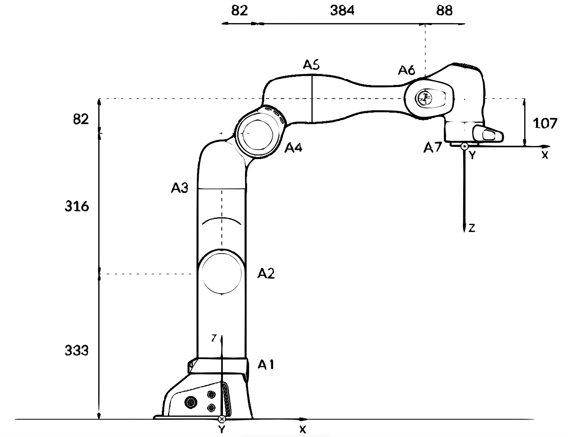
Figure 1: Axes and joint lengths [mm] of the Franka Emika robot [32].

The Franka Emika robotic arm boasts a 7-axis configuration, providing a 3 kg payload capacity and an impressive reach of 850 mm. The robot weighs approximately 18 kg and its repeatability is 0.1 mm. Repeatability is a measure of the ability of the robot to consistently reach a specified point. The robot works as a torque-controlled robot, using strain gauges to measure forces on all of its seven joints. Fig. 1 shows the axes and joint lengths of a Franka Emika robotic arm [32].

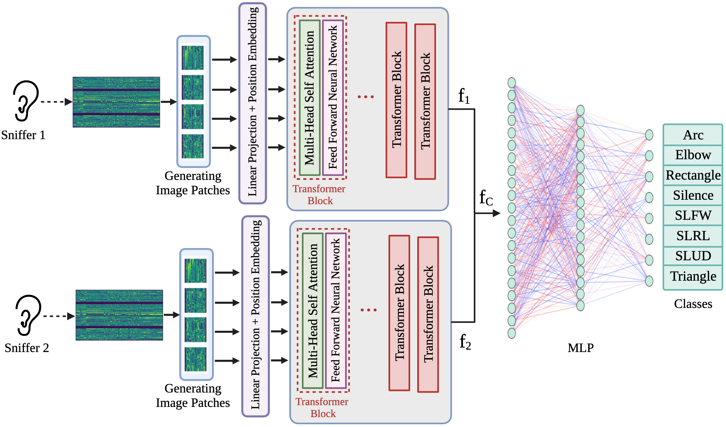
Figure 2: The architecture of BiVTC model. CSI data of each sniffer are separately patched, encoded, and then fed to transformer blocks for feature extraction. Then, the features are concatenated and imported as input of MLP. $f_{1}$ and $f_{2}$ are the features extracted from each stream of data.

III Proposed Methods

Studying the amplitude of CSI data and images reveals several commonalities in data analysis and machine learning. Despite the differences in their nature and applications, the common thread of data representation, spatial insight, and feature extraction underscores the fundamental approaches to analyzing and learning from CSI data and images, hence we apply vision-based methods to analyze the collected data and classify them to different types of robotic activities. The first method applied to our data is a CNN and the proposed architecture is constructed to effectively capture hierarchical features from CSI samples and generalize well across diverse datasets. The architecture comprises a series of convolutional, pooling, and fully connected layers, along with appropriate regularization techniques.
Another deployed model to study the collected CSI data is a vision transformer [33]. Departing from the conventional CNNs, the ViT harnesses the potency of self-attention mechanisms, which have demonstrated remarkable success in natural language processing tasks. At its core, the ViT architecture brings a novel perspective to the analysis of CSI data. This innovative approach transforms the CSI data into sequences of smaller data segments, similar to patches in image data. This transformation enables harnessing the power of self-attention mechanisms, which excel at capturing intricate relationships between different segments.

To explain the architecture of our algorithm, BiVTC, we begin by revisiting the attention mechanism employed in the original vision transformers [33]. The mathematical foundation of the ViT model rests on the self-attention mechanism. Self-attention, represented by the following formula

$$\text{Attention}(\mathbf{Q},\mathbf{K},\mathbf{V})=\sigma\left(\frac{\mathbf{Q}\mathbf{K}^{\top}}{\sqrt{d_{k}}}\right)\mathbf{V},$$ (4)

where $\sigma(\cdot)$, $\mathbf{Q}$, $\mathbf{K}$, and $\mathbf{V}$ denote the Softmax function, query, key, and value matrices, which these values are the amplitude information derived from CSI patches, and $d_{k}$ is the dimension of the key vectors, which captures the essence of relationships between different patches in CSI data.

Patch set for each CSI sample is achieved by reshaping the input sample $\mathbf{A}\in\mathbb{R}^{s\times t}$ to $\mathbf{A}_{p}\in\mathbb{R}^{N\times P\times P}$, where $P$ is height and width of $patch_{i}$, and $N=\frac{st}{P^{2}}$ presents number of patches in one CSI sample, then each patch is flattened to the shape $x_{p}\in\mathbb{R}^{P^{2}}$. Going through positional encoding and embedding the input sequence gets mapped to a vector of shape $\nu$, which is the same as the model and hidden state dimension size.

The representations of these CSI patches are then channeled through a sequence of transformer layers, each equipped with multi-head self-attention (MHSA). This architectural arrangement empowers the model to discover both local patterns and global contexts within the CSI amplitude data, thereby making it proficient in understanding the positions and interactions of key subcarrier components. The MHSA operation involves concatenating the outputs of attention heads and linearly projecting them to generate the final attention output. Mathematically, MHSA can be represented by

$$\text{MultiHead}(\mathbf{Q},\mathbf{K},\mathbf{V})=\big{(}\lambda_{1}\odot\lambda_{2}\ldots\odot\lambda_{M}\big{)}\mathbf{W}_{O},$$ (5)

where $\odot$ denotes the concatenation operation and $M$ is the number of attention heads $\lambda$,

$$\lambda_{i}=\text{Attention}(\mathbf{Q}\mathbf{W}_{Qi},\mathbf{K}\mathbf{W}_{Ki},\mathbf{V}\mathbf{W}_{Vi}).$$ (6)

In (6), $\mathbf{W}_{Qi},\mathbf{W}_{Ki},\mathbf{W}_{Vi}\in\mathbb{R}^{\nu\times\frac{\nu}{m}}$ are query, key, and value weight matrices per head, and $\mathbf{W}_{O}\in\mathbb{R}^{\nu\times\nu}$ is the output weight matrix, respectively. In each transformer block, a multi-layer perceptron (MLP) with GeLU activation function operates element-wise on each embedded output of MHSA. In the BiVTC model, we applied the computationally efficient ReLU activation function. The ViT model, on the other hand, aggregates these operations across multiple layers to progressively extract hierarchical features from image patches. In our study, where we process data from two distinct sniffers, we employ two separate ViT networks ($\mathcal{V}_{1}$ and $\mathcal{V}_{2}$), yielding different feature sets, denoted as $f_{1}$ and $f_{2}$, as illustrated in Fig. 2.

In the final step of the BiVTC model, we concatenate $f_{1}$ and $f_{2}$, forming a combined feature set as

$$f_{C}=f_{1}\odot f_{2}.$$ (7)

This concatenated feature set $f_{C}$ is then the input to an MLP for the classification of various robotic activities.

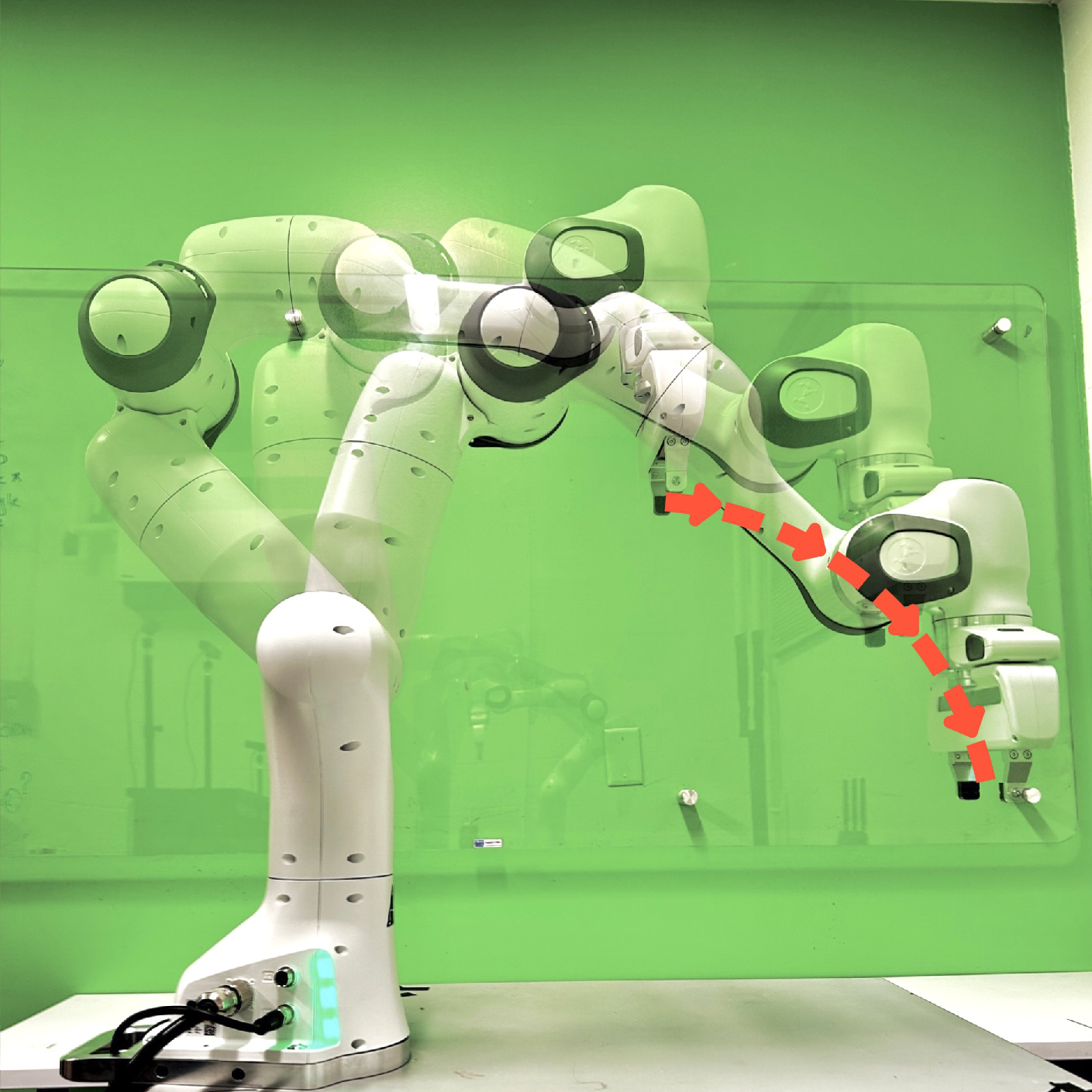
(a) Arc

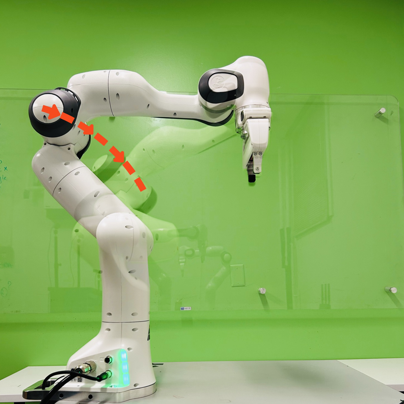
(b) Elbow

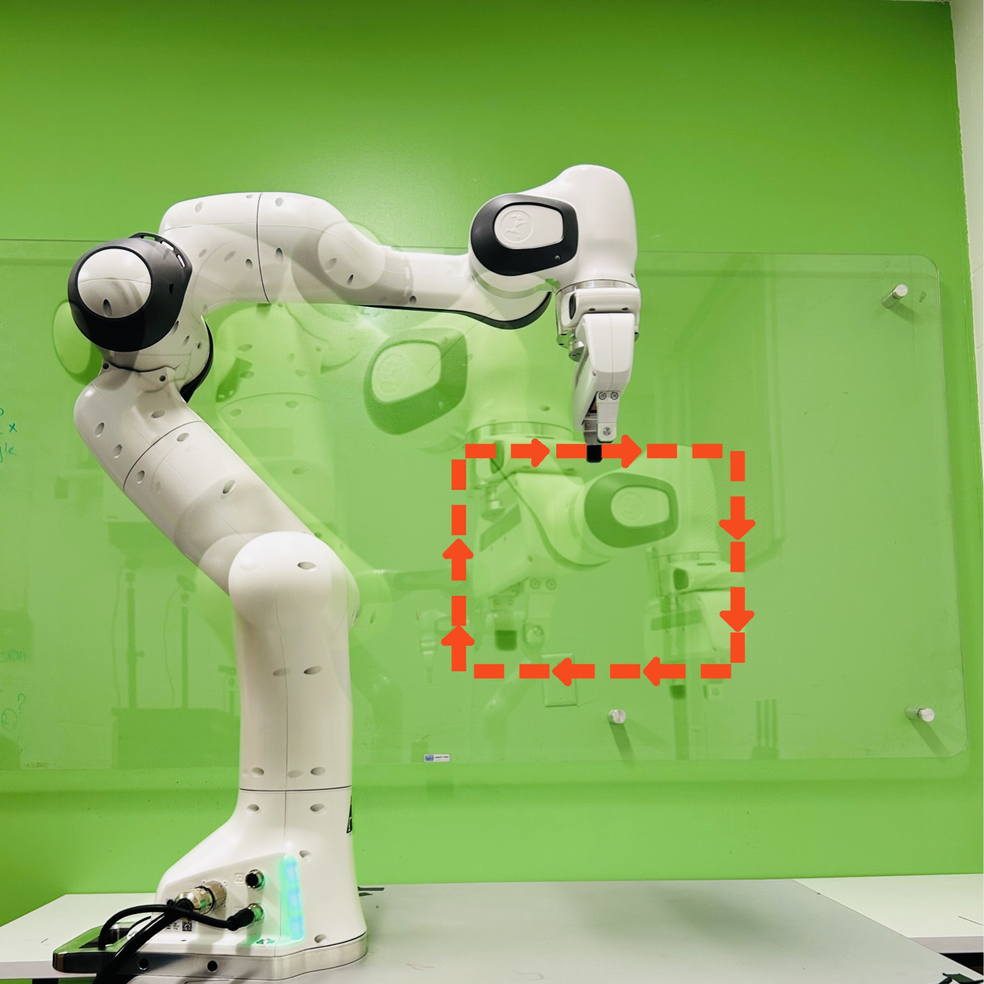
(c) Rectangle

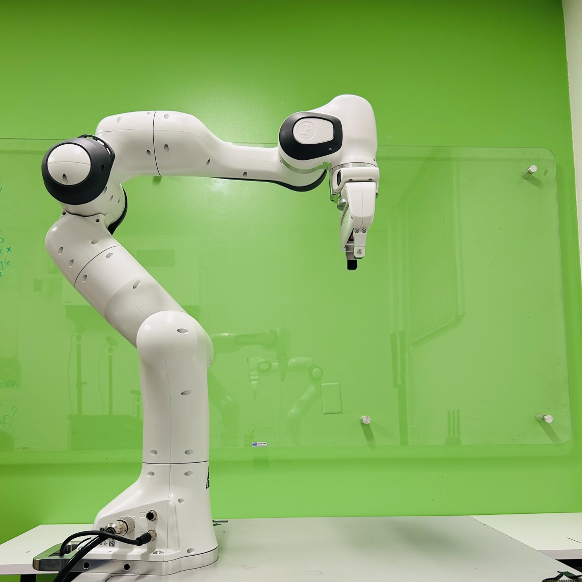
(d) Silence

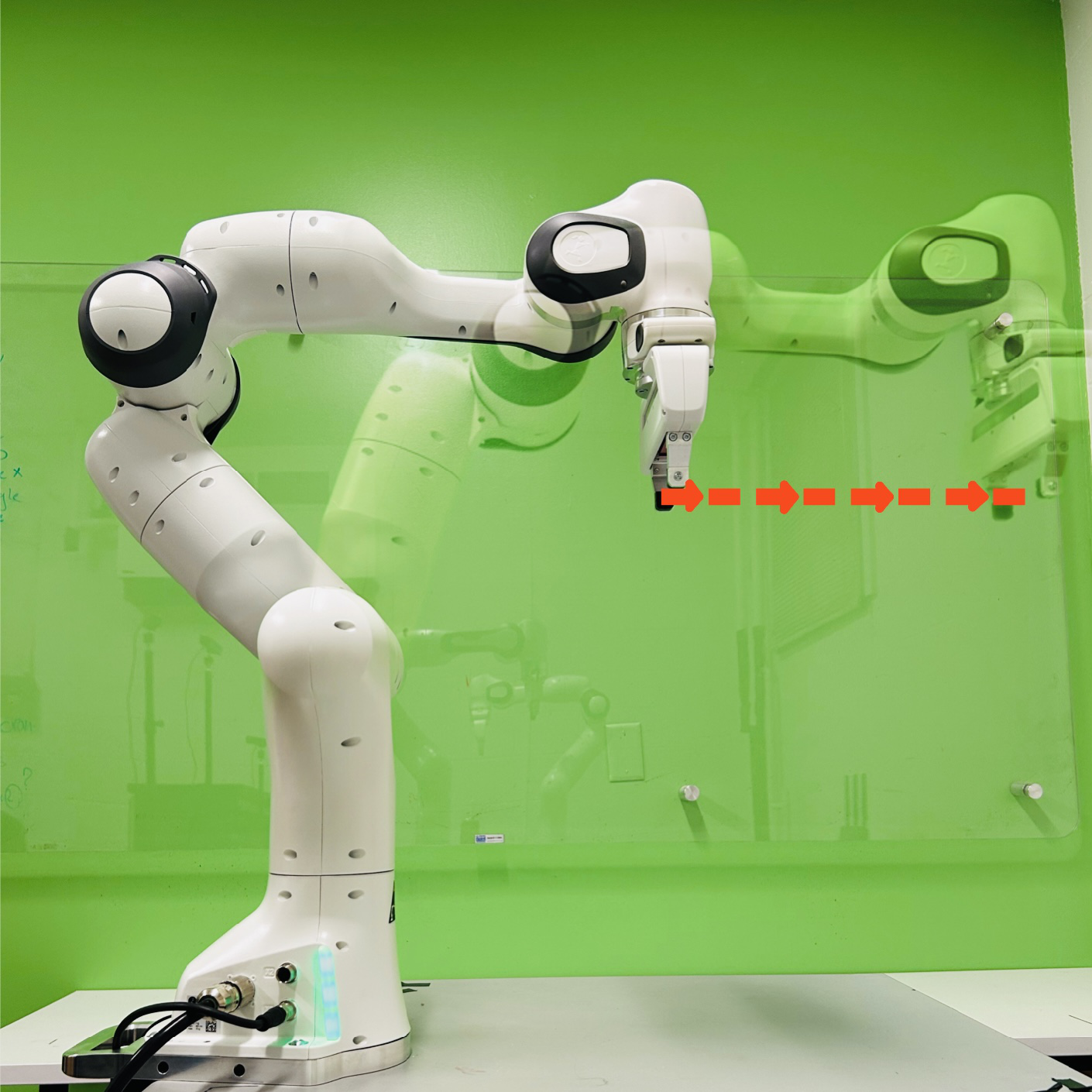
(e) SL-Forward

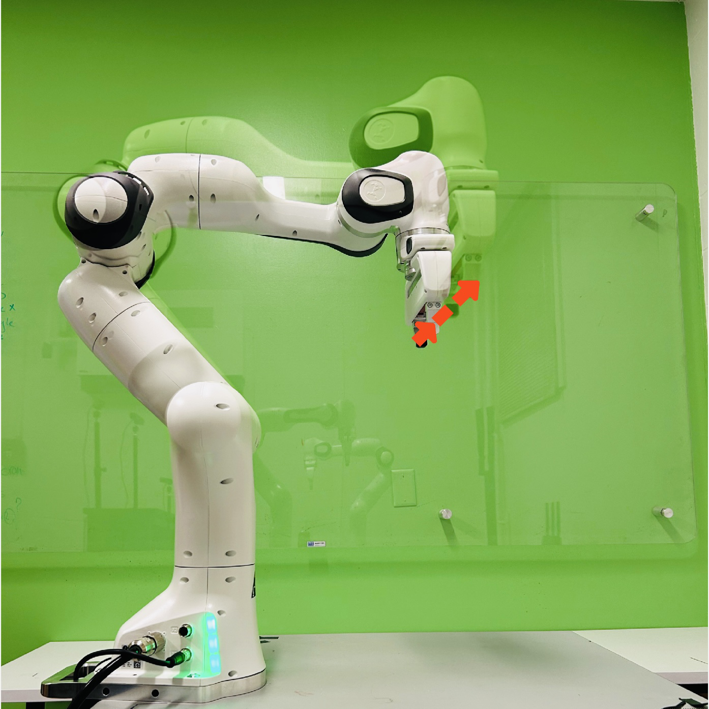
(f) SL-Right Left

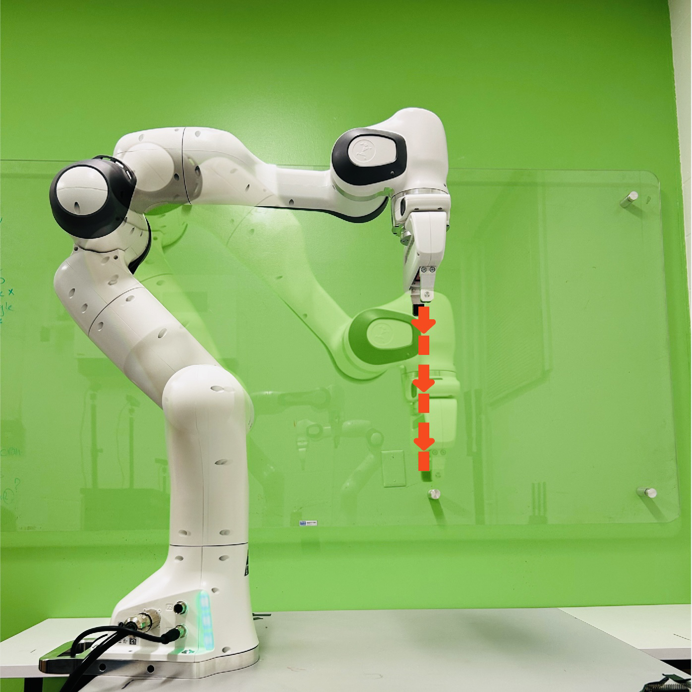
(g) SL-Up Down

(h) Triangle

Figure 3: Illustration of the eight activities performed by the Franka Emika arm in the experiments: (a) Arc, (b) Elbow, (c) Rectangle, (d) Silence, (e) Straight Line - Forward (SLFW), (f) Straight Line - Right Left (SLRL), (g) Straight Line - Up Down (SLUD), and (h) Triangle. The motion patterns of the robotic arm are shown with red dashed lines.

IV RoboFiSense Dataset

IV-A Data Collection

The process of data collection encompassed the acquisition of CSI through two sniffers placed at distinct locations within the room. The transmission of WiFi signals employed an 80 MHz bandwidth, facilitating the capture of 256 sub-carriers by each sniffer at every timestamp. Operating at a sampling rate of 30 Hz, data collection occurred over a 12-second interval, yielding a collection of CSI matrices denoted as $\mathbf{H}\in\mathbb{C}^{256\times 360}$ prior to preprocessing. Notable preprocessing steps include the exclusion of pilot and unused subcarriers [34], followed by the computation of CSI value amplitudes. Consequently, this process led to a reduction in matrix size, yielding $\mathcal{\mathbf{A}}\in\mathbb{R}^{232\times 360}$ for each sample. Noteworthy is the fact that the most prolonged activity sequences in our dataset spanned up to four seconds, with the occurrence of activities transpiring at random intervals within the 0 to 8-second time-frame.

In our RoboFiSense dataset, we study eight different activities of a Franka Emika robot; (a) Arc, (b) Elbow, (c) Rectangle, (d) Silence, (e) Straight Line - Forward (SLFW), (f) Straight Line - Right Left (SLRL), (g) Straight Line - Up Down (SLUD), and (h) Triangle. The activity paths of the robotic arm are shown with red dashed lines in Fig. 3. We have released this dataset, making it accessible to the public and contributing valuable resources to the research society in the course of their studies.
In section V, we investigate the impact of both robotic activity velocity and the placement of sniffers for data collection on the effectiveness of our machine learning algorithms. To achieve this, our dataset encompasses three distinct velocity levels, each of which incorporates a 10% increase in both velocity and acceleration. For our study on the placement of sniffers, we devised a grid consisting of nine unique locations—a $3\times 3$ grid configuration. In each experimental scenario, our two sniffers were strategically relocated to different positions within this grid. Notably, one location within the grid was continually occupied by our stationary robot, ensuring that it remained static. This configuration allowed us to explore four distinct scenarios of data collection. Refer to Fig. 4 for a visual representation of the grid map.

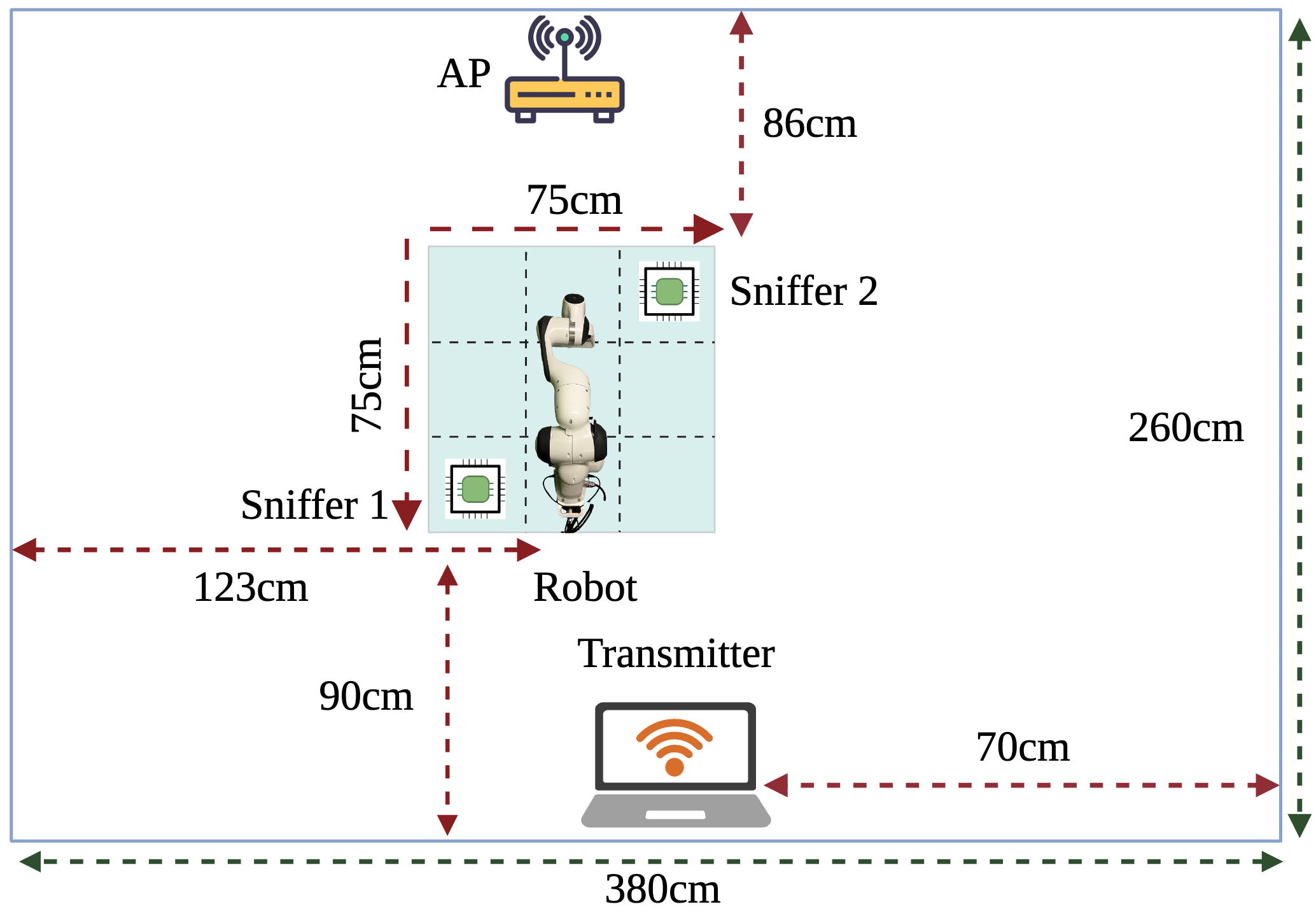
Figure 4: Floor plan of data collection environment. The grid area provides an overview of various sniffer placement options. As depicted in the image, two sniffers are positioned at location 1 as an illustrative example.

IV-B Setup

We employed a dual Raspberry Pi 4 setup, integrating the Nexmon project [35] to procure comprehensive CSI data from our sniffer devices. Each Raspberry Pi, equipped with Nexmon, facilitated CSI data acquisition, incorporating local timestamping directly on the hardware. The timestamped data is then sent to the loop-back interface of the network. While this configuration effectively captures data from individual sniffers, the synchronization of timestamps becomes crucial for multi-sniffer deployments. Addressing this requirement, we devised a solution where loop-back packets containing CSI data from each Raspberry Pi are redirected to a dedicated system, referred to as the monitor.

The monitor functions as a central hub, gathering packets from various sniffers and applying synchronized timestamps as dictated by a designated frequency.

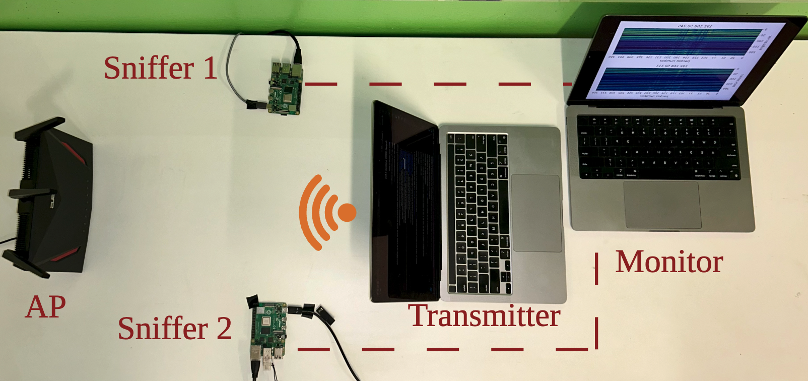
(a) Real setup

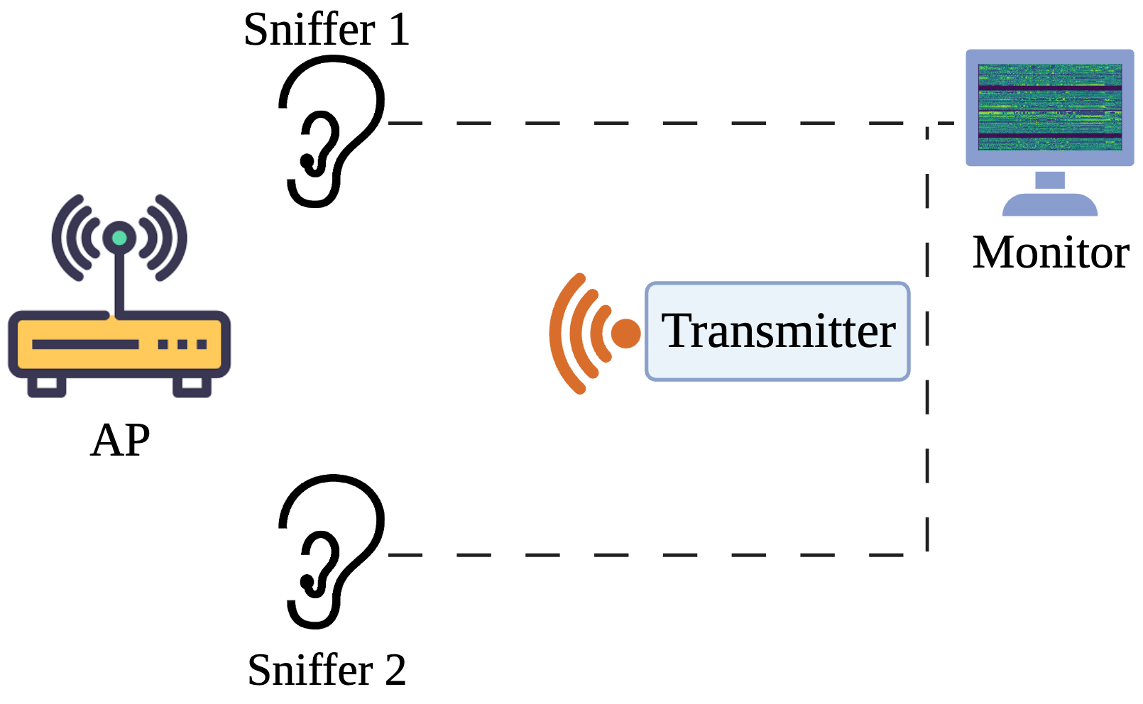
(b) Schematic map of the setup

Figure 5: (a) and (b) depict real and schematic maps illustrating the communication flow between sniffers and the monitor. In this setup, the sniffers capture the packets sent by the transmitter. After the CSI extraction is done by the sniffers, the sniffers send the extracted CSI information to the monitor, to be stored, timestamped, and further processed.

A visual representation of this intercommunication is presented in Fig. 5.

(a) Sample One

(b) Sample Two

Figure 6: Synchronized CSI collection from two sniffers. The distortion comes from a sudden movement in the environment captured by both sniffers at the correct time. (a) and (b) are two different samples, each of them captured from two sniffers.

It is worth noting that in line with the Nexmon project’s specifications, Raspberry Pis operating as sniffers lose WiFi communication capability. To circumvent this limitation, we interconnect the sniffers and the monitor via Ethernet cables, ensuring seamless communication between the sniffers and the monitor. The concluding color map illustrates the $\mathbf{A}$ matrices extracted from both sniffers, as depicted in Fig. 6. This visual representation showcases their synchronized timeline, capturing instances of CSI packet distortions resulting from sudden activities during a specific time interval, as observed by both CSI sniffers.

V Experiments

V-A Model Diversity

To have a comparison on the performance of different models, we employed CNN, ViT, and our own designed model BiVTC, which was discussed in section III. In the architecture of the CNN model, the initial layers consist of convolutional layers that employ rectified linear unit (ReLU) activation functions to introduce non-linearity [36]. The subsequent layers are equipped with max-pooling operations to down-sample the spatial dimensions, aiding in reducing the computational complexity while retaining the most relevant features.

To prevent overfitting, we have integrated ${L}_{2}$ regularization into specific convolutional layers. The regularization coefficients are empirically determined through experimentation on the dataset to ensure an optimal trade-off between preventing overfitting and preserving feature richness. Additionally, dropout layers are strategically placed within the network to further enhance generalization capabilities.

Furthermore, we adopt an early stopping mechanism with a patience of 15 epochs to mitigate overfitting during training. The model’s performance is evaluated using categorical cross-entropy loss and accuracy metrics during both the training and validation phases.

(a) Number of transformers layers and batch size

(b) Learning rate and dropout

Figure 7: Grid search on hyperparameters of ViT model. The values in the color-map present the validation accuracy (%).

The ViT model is configured with a set of hyperparameters tailored to optimize its performance. The patch size is defined as 45, determining the dimensions of CSI patches used for processing. A batch size of 16 is employed during training to balance computational efficiency and model convergence. As deployed in the CNN model, training occurs over 150 epochs with the same patience for the early stopping mechanism, allowing the model to learn from the dataset iteratively. With eight classes in the classification task, the model’s final fully connected layer accommodates this number for accurate class predictions. To facilitate training, a relatively low learning rate of $1\times 10^{-4}$ is used, with weight decay set at $2\times 10^{-5}$ to control overfitting. The ViT architecture incorporates four attention heads and a stack of six transformer layers to capture intricate spatial dependencies within the image data. To choose the proper number of transformer layers and batch size, we have done a grid search, as shown in Fig. 7. Dropout regularization with a rate of 0.4 is strategically applied throughout the network to enhance generalization and prevent overfitting. These hyperparameters are fine-tuned to ensure the ViT model’s optimal performance on CSI data classification tasks.

Incorporating the concepts from ViT, the BiVTC model takes this approach a step further by employing two vision transformers, each tailored to capture distinctive features from the different sniffers. These features are then fused through concatenation, providing the model with a richer representation to enhance classification accuracy. This capacity is pivotal in recognizing unique spatial structures present in the data. The choice of the parameters of BiVTC is based on the grid search done in the ViT model.

V-B Studying Different Velocities

Examining the repercussions of diverse velocities within HAR introduces inherent challenges. Ensuring consistent control over human activity speeds across data collection from various individuals is intricate. To overcome this obstacle, we adopted an innovative strategy. We systematically manipulated the robot’s velocity for all activities during data collection. This method allowed us to scrutinize the dataset under precisely controlled velocity conditions.

The data of each activity was gathered across three distinct velocities and accelerations: $V_{1}$, $V_{2}$, and $V_{3}$. Velocity $V_{1}$ embodies the slowest pace, while $V_{2}$ is 10% quicker, and $V_{3}$ escalates by 20% compared to $V_{1}$. In this experimental paradigm, we trained our CNN, ViT, and BiVTC models using two of these velocities, subsequently testing their efficacy on a distinct velocity set. Our overarching objective was to cultivate a robust model capable of accurately classifying varied robot activities across a spectrum of velocities.

V-C Sniffer Location Selection

Choosing the best sensor location in robotics represents a prominent and actively explored research field, as highlighted by Shi et al. [37]. As discussed earlier, WiFi sensing is highly dependent on location, and to tackle this issue we need to collect a large amount of data in different environments to develop a robust model for changes in the environment, as done in [16]. This issue raises a question about selecting the best location to place the sniffers, to obtain rich data of the activities happening in the environment. To study the effect of sniffer location, we have built a $3\times 3$ grid area and located the sniffers strategically in different locations, as illustrated in Fig. 4.

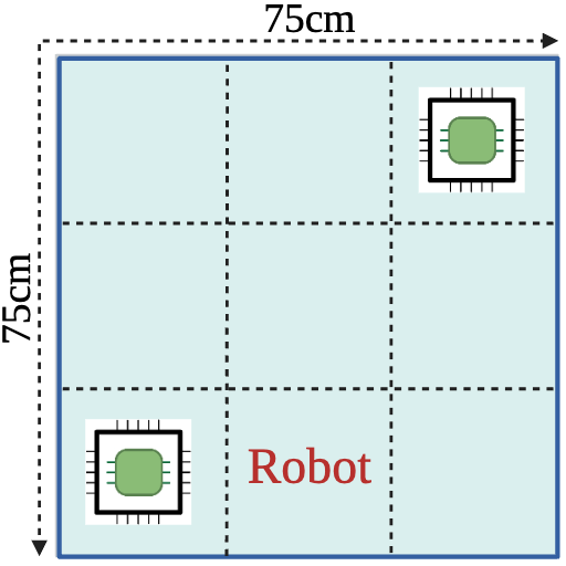
(a) $L_{1}$

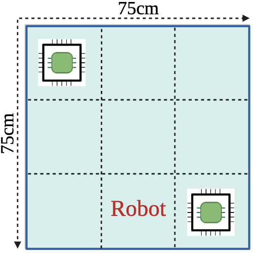
(b) $L_{2}$

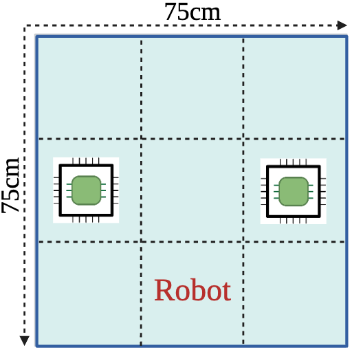
(c) $L_{3}$

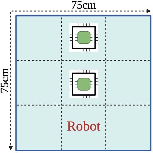
(d) $L_{4}$

Figure 8: A $3\times 3$ grid area and four different locations of sniffers. There are nine locations in the grid, which one is always occupied by the base of the robot, so there remain eight grid cells for two sniffers, resulting in a set of four distinct locations, $\mathcal{S}_{L}=\{L_{1},L_{2},L_{3},L_{4}\}$. At each round of data collection, we move the sniffers to a new location, resulting in four different sets of data collected from distinct locations.

There are nine locations in the grid, which one is always occupied by the base of the robot, so there remain eight grids for two sniffers. Having eight locations and two sniffers, where the order does not matter, gives us 28 different combinations of sniffer locations. We also aim to avoid placing the sniffers in close proximity to each other (i.e., in the same grid cell). With two sniffers, our objective is to gather CSI data from distinct locations, enhancing the robustness of our model. Following a grid search for suitable locations, we opted to position our sniffers in four different areas denoted as $\mathcal{S}_{L}={\{L_{1},L_{2},L_{3},L_{4}\}}$, as presented in Fig. 8.

Our primary objective is to investigate the impact of location within a robotic environment through the analysis of learning curves and the evaluation of test results for each location. Ultimately, our aim is to identify the optimal location for the sniffers to collect a comprehensive dataset, and compare the required time and computational power to achieve high accuracy. As our final study, we experiment with the effect of adding data of different locations, as a regularization method, to decrease the overfitting of the model and increase the performance on the test set.

VI Results and Analysis

As outlined in Section V-A, we have employed various models, namely CNN, ViT, and BiVTC, to thoroughly investigate our collected data and facilitate result comparisons. Our dataset incorporates samples obtained at different velocities ($V_{1}$, $V_{2}$, and $V_{3}$). We used collected samples with velocity $V_{2}$, and each of these models were trained on 80% of $V_{2}$ set and subsequently subjected to testing on the remaining 20%. The results, detailed in Table II, showcase the average and standard deviation of classification metrics, derived following a rigorous 5-fold cross-validation process.

Table I: Average accuracy of each class of activity for CNN, ViT, and BiVTC, trained on two velocities and tested on another velocity, at location 1, in percentage (%).

Train	Test	Model	Arc	Elbow	Rectangle	Silence	SLFW	SLRL	SLUD	Triangle	All
$V_{1}$$V_{2}$	$V_{3}$	CNN	86.21	26.09	56.52	83.02	28.62	34.78	86.96	84.92	60.33
		ViT	78.26	89.14	73.26	78.26	50.00	63.04	30.43	82.61	68.20
		BiVTC	97.39	93.04	89.57	97.39	73.04	63.48	89.57	96.52	87.50
$V_{1}$$V_{3}$	$V_{2}$	CNN	65.22	82.61	39.13	100.00	100.00	17.39	43.48	95.65	67.93
		ViT	86.96	47.83	52.17	91.30	100.00	82.61	91.30	26.09	72.28
		BiVTC	100.00	82.61	91.30	100.00	65.22	100.00	78.26	78.26	86.96
$V_{2}$$V_{3}$	$V_{1}$	CNN	67.80	21.74	30.43	100.00	73.91	73.91	86.96	73.91	68.47
		ViT	39.13	73.91	43.48	95.65	100.00	52.17	95.65	47.83	68.48
		BiVTC	75.65	60.00	62.61	100.00	100.00	93.04	97.39	90.43	84.89

Table II: Average and Standard deviation of precision, recall, F1-score and accuracy of CNN, ViT and BiVTC, trained on $V_{2}$ with 80% train set and 20% test set division, at location 1, in percentage (%).

Model	Precision	Recall	F1-Score	Accuracy
CNN	84.63 $\pm$ 3.19	83.15 $\pm$ 2.36	82.43 $\pm$ 3.47	83.15 $\pm$ 2.36
ViT	91.27 $\pm$ 1.22	90.76 $\pm$ 2.61	90.51 $\pm$ 2.78	90.76 $\pm$ 2.61
BiVTC	93.33 $\pm$ 2.23	92.50 $\pm$ 2.45	92.45 $\pm$ 2.91	92.50 $\pm$ 2.45

It is noteworthy that, owing to the balanced number of samples in each class of our dataset, accuracy and recall metrics are equivalent. The discerning observation is that our BiVTC algorithm consistently outperforms both the CNN and ViT models.

In another experiment, we analyze the robustness of the deployed models to variations in velocity and acceleration. In this series of experiments, we maintained consistent locations and types of activities, with the sole variations occurring in speed and acceleration parameters. Each model undergoes training on two distinct sets of velocities and is subsequently evaluated on a separate test set. Table I provides the average accuracy of each class, derived from 5-fold cross-validation across all models. The first two columns in the table denote the velocity sets used for both training and testing.

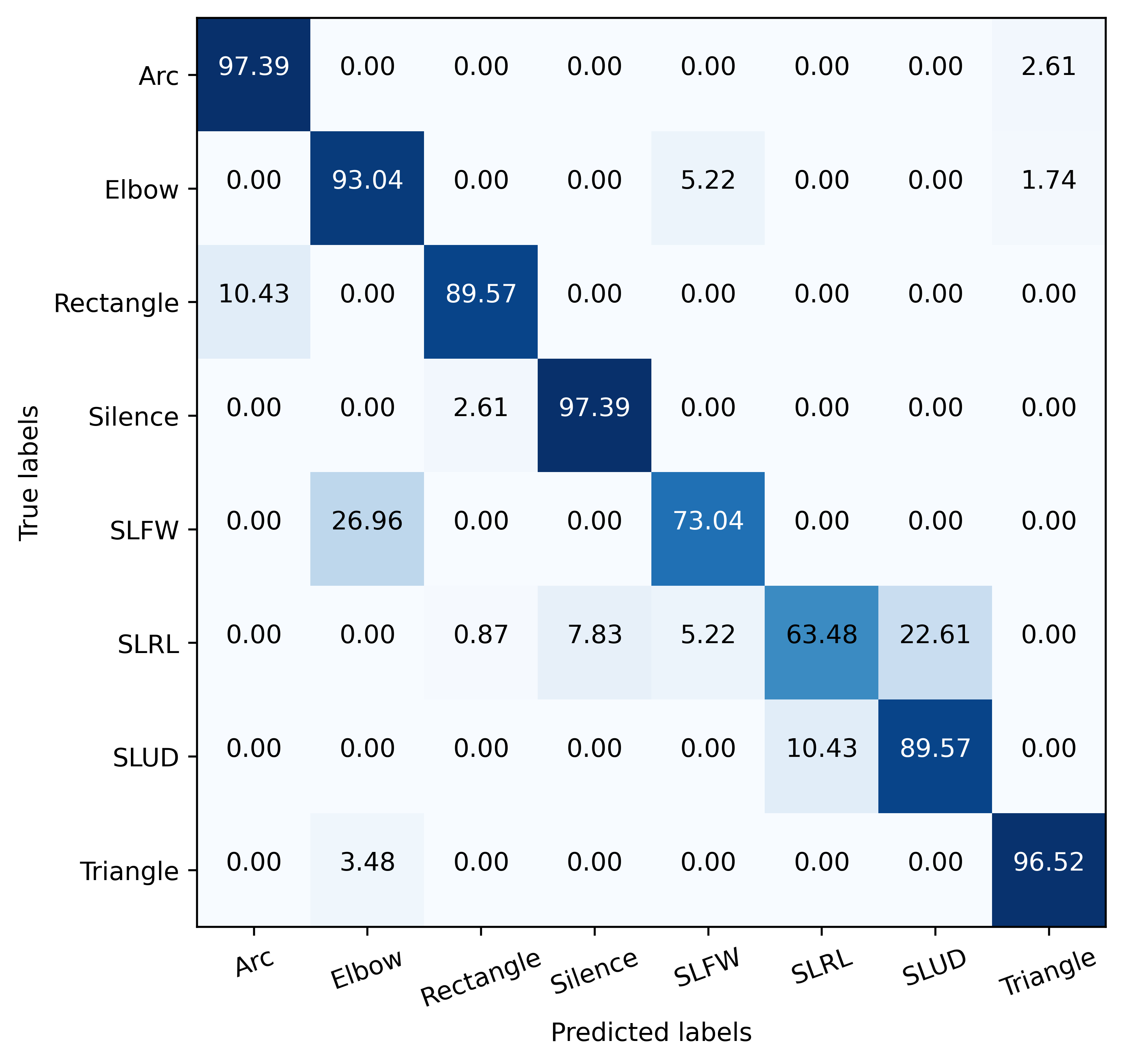
(a) Trained on $V_{1}$$V_{2}$ - Tested on $V_{3}$

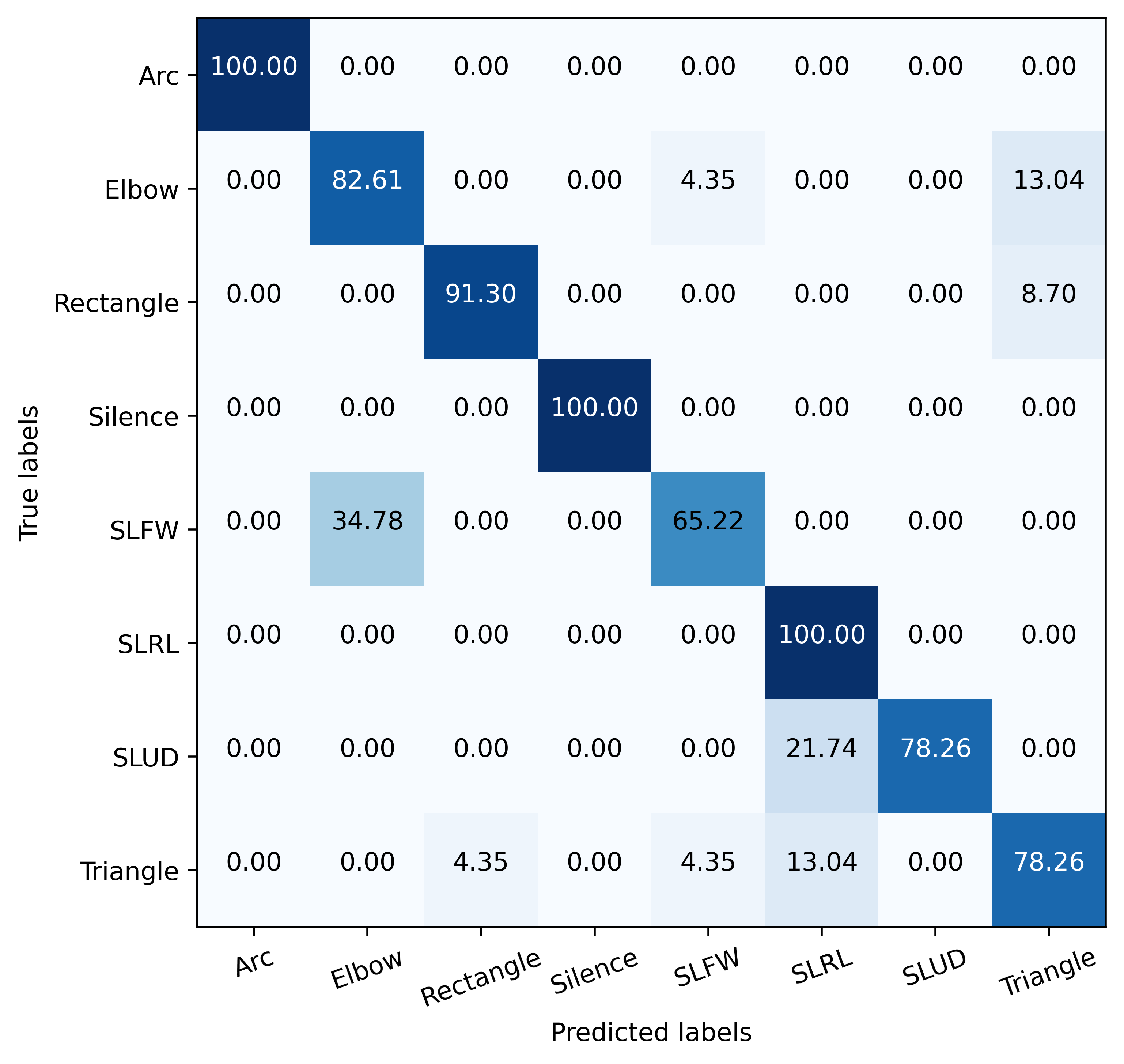
(b) Trained on $V_{1}$$V_{3}$ - Tested on $V_{2}$

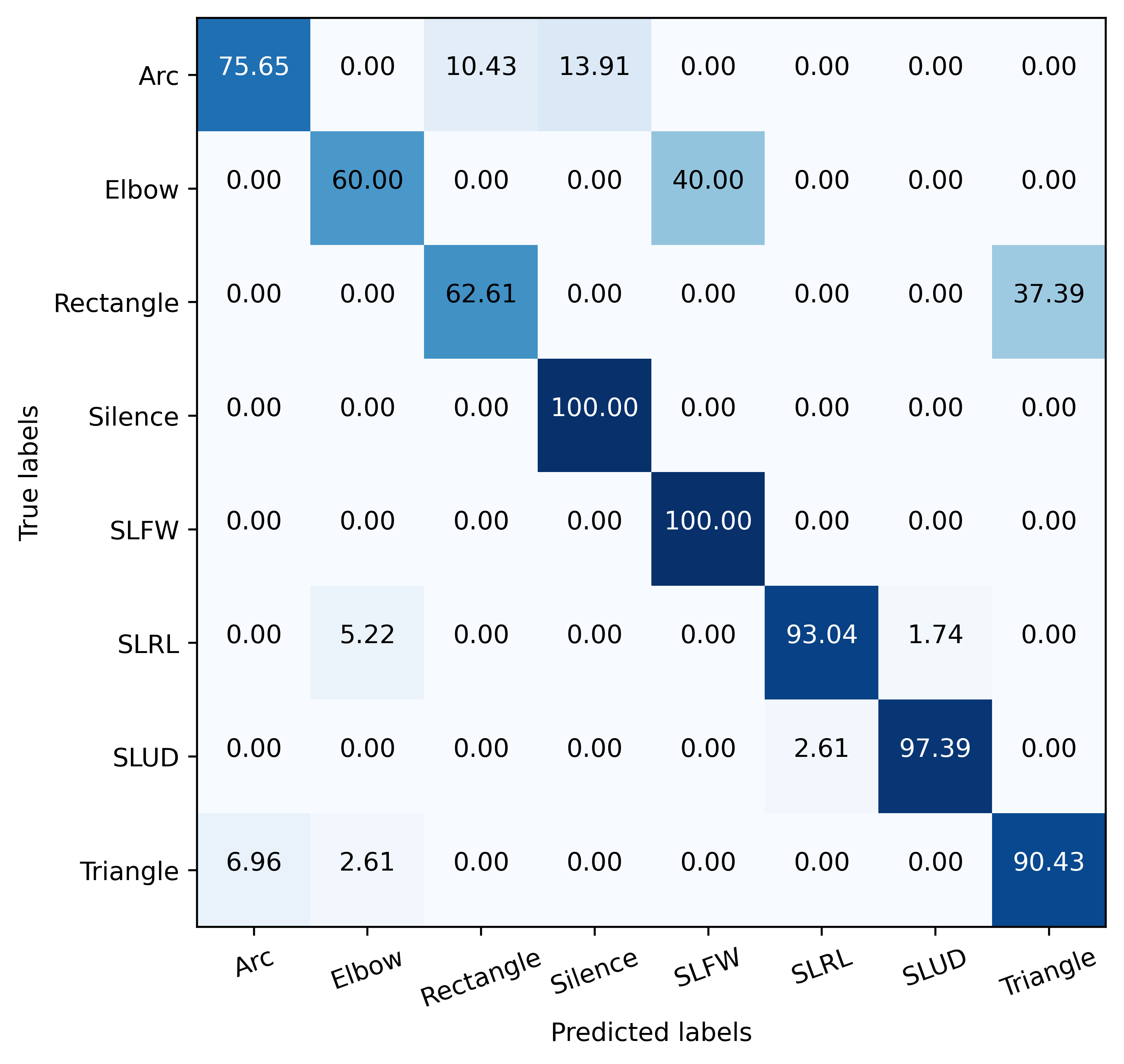
(c) Trained on $V_{2}$$V_{3}$ - Tested on $V_{1}$

Figure 11: The averaged 5-fold cross-validated confusion matrices of BiVTC model, trained and tested on different sets of velocities.

In Table III, we report the average classification metrics for BiVTC, presented as percentages along with their standard deviations. Notably, BiVTC demonstrates promising results in the recognition of robotic activity under diverse velocity and acceleration conditions. To have a better understanding of the BiVTC model performance we present the confusion matrices of the model tested on three different velocities, in Fig. 11 (see the Appendix).

Table III: Average and standard deviation of precision, recall, and F1-score of BiVTC trained and tested on different sets of velocities, at location 1, in percentage (%).

Train	Test	Precision $(\%)$	Recall $(\%)$	F1-Score $(\%)$
$V_{1}$ & $V_{2}$	$V_{3}$	88.71 $\pm$ 2.60	87.50 $\pm$ 2.40	87.08 $\pm$ 2.13
$V_{1}$ & $V_{3}$	$V_{2}$	88.31 $\pm$ 1.78	86.96 $\pm$2.06	86.95 $\pm$ 2.48
$V_{2}$ & $V_{3}$	$V_{1}$	86.46 $\pm$ 2.97	84.89 $\pm$ 3.19	84.42 $\pm$ 3.46

To address the challenge of identifying the most suitable sniffer placement for reliable environmental modeling, we strategically deployed sniffers throughout a grid region to examine the influence of location on the gathering of activity data, as shown in Fig. 8. We collected 18 training and five test CSI samples of each class of robotic arm activity from each of those four different locations, all with a velocity of $V_{2}$, resulting in four training and four test sets. Thus, the only variable across these datasets is the location of the sniffers.

In the first step, we trained the BiVTC model in one location and tested it in the same location. The test accuracy for each location is presented as the first bar in the bar plots of Fig. 9. To gain a better understanding of the data, we also studied the training process for each location by providing learning curves. Fig. 10 illustrates the loss and accuracy curves for both training and validation sets for each location. Let’s discuss the model’s performance in training, validation, and testing for all four locations.

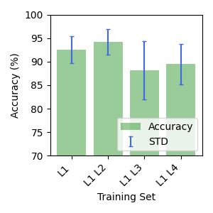
(a) Testing on $L_{1}$

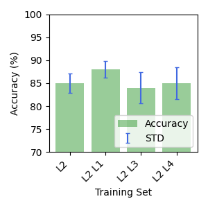
(b) Testing on $L_{2}$

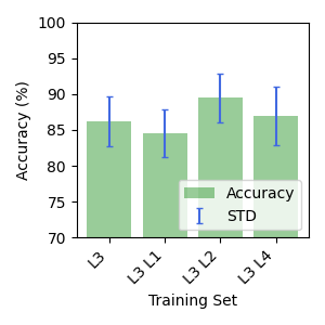
(c) Testing on $L_{3}$

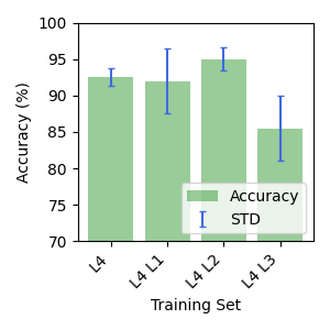
(d) Testing on $L_{4}$

Figure 9: Average and standard deviation of the accuracy of testing different locations on BiVTC. In each plot, we tested our model on one distinct location, while changing the training set (X-Axis), to have a comparison between different locations and the effect of dynamically augmenting the training data.

In Location 1 ($L_{1}$), between the $60^{\text{th}}$ and $70^{\text{th}}$ epochs, the training and validation accuracy averaged 94.3% and 92.6%, respectively, with the loss dropping to less than 0.5. By epoch 150, the training accuracy reached 96.4%, and the BiVTC model achieved a test accuracy of 92.5%. Notably, the validation loss closely followed the training loss.

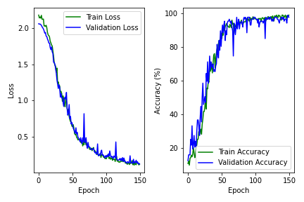
(a) Testing on $L_{1}$

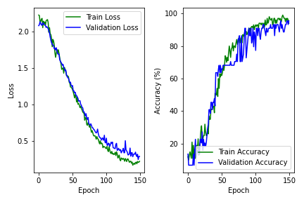
(b) Testing on $L_{2}$

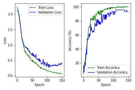
(c) Testing on $L_{3}$

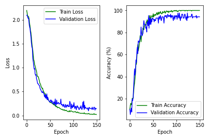
(d) Testing on $L_{4}$

Figure 10: Learning curves of BiVTC model, tested on different locations. Each figure presents train and validation loss and accuracy, for one distinct location. In this scenario, the model is trained and tested on the data of the same location.

In Location 2 ($L_{2}$), the learning curves exhibited a slower slope, indicating that learning data from this location required more time, which can be challenging with limited time and memory resources. This slower learning process also affected the test accuracy, which dropped to 85.0%.

In the case of Location 3 ($L_{3}$), there was approximately a 15.0% difference between test and validation accuracy, which was more pronounced in the loss plot. This difference was also reflected in the lower test accuracy of 86.2%. It is notable, in training our models, we have used early stopping and dropout to prevent overfitting, as discussed in section V-A, so the results shown in Fig. 10 are only for sake of comparison, and what we observe in between epoch $120^{\text{th}}$ to $150^{\text{th}}$ is prevented the original design of the model.

Finally, in Location 4 ($L_{4}$), which is the closest location to the robotic arm’s body, we observed a steep slope in both the validation and training curves. Additionally, the test accuracy for $L_{4}$ increased to 91.5%, highlighting the simplicity of this dataset.

To augment the dataset, we mixed the training sets and assessed whether adding data from different locations could improve the model’s performance in recognizing activities in the test set. As shown in Fig. 9, adding data from $L_{2}$ proved beneficial for the model across all locations, functioning as a regularization method that contributed to higher accuracy.

VII Conclusion

Within the domain of autonomous robotics, the precise prediction of robot activity within indoor environments marked by limited visibility presents an enduring challenge. Conventional methods for detecting and localizing robotic arm activity have predominantly relied on vision-based or LiDAR sensors, raising privacy concerns and imposing strict line-of-sight (LoS) requirements for accuracy. In scenarios where supplementary sensors are unavailable, or LoS is unattainable, these approaches often prove less effective.

This study presents a novel approach that utilizes CSI extracted from WiFi signals which are subtly influenced by the activity of robotic arms. Our implementation known as the BiVTC methodology demonstrates the capability to effectively classify eight distinct activities performed by a Franka Emika robotic arm. Notably, our approach excels in recognizing robotic arm activities with precision, regardless of whether it is trained on activities with varying velocities, all without the dependency on external or internal sensors or visual aids.

For the benefit of future research and to promote community collaboration, we have collected a comprehensive CSI dataset containing the motion data of eight robotic activities. This dataset has been published, making it accessible to the public and providing valuable resources to researchers worldwide. By leveraging the inherent properties of WiFi signals, our research introduces a pioneering dimension to the prediction of autonomous robotic activity in challenging indoor environments, thereby paving the way for future advancements in this field. [Average confusion matrices of BiVTC model]

References

- [1] Christopher G Atkeson et al. “No falls, no resets: Reliable humanoid behavior in the DARPA robotics challenge” In 2015 IEEE-RAS 15th International Conference on Humanoid Robots (Humanoids), 2015, pp. 623–630 IEEE
- [2] Sami Haddadin, Alessandro De Luca and Alin Albu-Schäffer “Robot collisions: A survey on detection, isolation, and identification” In IEEE Transactions on Robotics 33.6 IEEE, 2017, pp. 1292–1312
- [3] Agostino De Santis, Bruno Siciliano, Alessandro De Luca and Antonio Bicchi “An atlas of physical human–robot interaction” In Mechanism and Machine Theory 43.3 Elsevier, 2008, pp. 253–270
- [4] Rainer Bischoff et al. “The KUKA-DLR Lightweight Robot arm-a new reference platform for robotics research and manufacturing” In ISR 2010 (41st international symposium on robotics) and ROBOTIK 2010 (6th German conference on robotics), 2010, pp. 1–8 VDE
- [5] Simona Aracri et al. “Soft robots for ocean exploration and offshore operations: A perspective” In Soft Robotics 8.6 Mary Ann Liebert, Inc., publishers 140 Huguenot Street, 3rd Floor New …, 2021, pp. 625–639
- [6] Anthony R Lanfranco, Andres E Castellanos, Jaydev P Desai and William C Meyers “Robotic surgery: a current perspective” In Annals of surgery 239.1 Lippincott, Williams,Wilkins, 2004, pp. 14
- [7] Seyed Farokh Atashzar et al. “Characterization of upper-limb pathological tremors: Application to design of an augmented haptic rehabilitation system” In IEEE Journal of Selected Topics in Signal Processing 10.5 IEEE, 2016, pp. 888–903
- [8] Mohd Javaid, Abid Haleem, Ravi Pratap Singh and Rajiv Suman “Substantial capabilities of robotics in enhancing industry 4.0 implementation” In Cognitive Robotics 1 Elsevier, 2021, pp. 58–75
- [9] Jing Li et al. “Building and optimization of 3D semantic map based on Lidar and camera fusion” In Neurocomputing 409 Elsevier, 2020, pp. 394–407
- [10] Matěj Petrlík, Tomáš Krajník and Martin Saska “LiDAR-based Stabilization, Navigation and Localization for UAVs Operating in Dark Indoor Environments” In 2021 International Conference on Unmanned Aircraft Systems (ICUAS), 2021, pp. 243–251 IEEE
- [11] Diogo Santos Ortiz Correa et al. “Mobile robots navigation in indoor environments using kinect sensor” In 2012 Second Brazilian Conference on Critical Embedded Systems, 2012, pp. 36–41 IEEE
- [12] Yongsen Ma, Gang Zhou and Shuangquan Wang “WiFi sensing with channel state information: A survey” In ACM Computing Surveys (CSUR) 52.3 ACM New York, NY, USA, 2019, pp. 1–36
- [13] Rojin Zandi et al. “Robot Motion Prediction by Channel State Information”, 2023 arXiv:2307.03829 [cs.RO]
- [14] Yu Gu et al. “MoSense: An RF-based motion detection system via off-the-shelf WiFi devices” In IEEE Internet of Things Journal 4.6 IEEE, 2017, pp. 2326–2341
- [15] Jian Liu et al. “Wireless sensing for human activity: A survey” In IEEE Communications Surveys & Tutorials 22.3 IEEE, 2019, pp. 1629–1645
- [16] Yue Zheng et al. “Zero-Effort Cross-Domain Gesture Recognition with Wi-Fi”, MobiSys ’19 Seoul, Republic of Korea: Association for Computing Machinery, 2019, pp. 313–325 DOI: 10.1145/3307334.3326081
- [17] Siamak Yousefi et al. “A Survey on Behavior Recognition Using WiFi Channel State Information” In IEEE Communications Magazine 55.10, 2017, pp. 98–104 DOI: 10.1109/MCOM.2017.1700082
- [18] Wondimu K Zegeye, Seifemichael B Amsalu, Yacob Astatke and Farzad Moazzami “WiFi RSS fingerprinting indoor localization for mobile devices” In 2016 IEEE 7th Annual Ubiquitous Computing, Electronics & Mobile Communication Conference (UEMCON), 2016, pp. 1–6 IEEE
- [19] Vicente Matellán Olivera, José María Cañas Plaza and Oscar Serrano Serrano “WiFi localization methods for autonomous robots” In Robotica 24.4 Cambridge University Press, 2006, pp. 455–461
- [20] Adrián Canedo-Rodríguez et al. “Particle filter robot localisation through robust fusion of laser, WiFi, compass, and a network of external cameras” In Information Fusion 27 Elsevier, 2016, pp. 170–188
- [21] Aichun Zhu et al. “Wi-ATCN: Attentional Temporal Convolutional Network for Human Action Prediction Using WiFi Channel State Information” In IEEE Journal of Selected Topics in Signal Processing 16.4, 2022, pp. 804–816 DOI: 10.1109/JSTSP.2022.3163858
- [22] Zhengjie Wang et al. “A survey on human behavior recognition using channel state information” In Ieee Access 7 IEEE, 2019, pp. 155986–156024
- [23] Zheng Yang, Zimu Zhou and Yunhao Liu “From RSSI to CSI: Indoor localization via channel response” In ACM Computing Surveys (CSUR) 46.2 ACM New York, NY, USA, 2013, pp. 1–32
- [24] Hojjat Salehinejad and Shahrokh Valaee “LiteHAR: lightweight human activity recognition from WIFI signals with random convolution kernels” In ICASSP 2022-2022 IEEE International Conference on Acoustics, Speech and Signal Processing (ICASSP), 2022, pp. 4068–4072 IEEE
- [25] Han Zou et al. “Adversarial learning-enabled automatic WiFi indoor radio map construction and adaptation with mobile robot” In IEEE Internet of Things Journal 7.8 IEEE, 2020, pp. 6946–6954
- [26] Joydeep Biswas and Manuela Veloso “Wifi localization and navigation for autonomous indoor mobile robots” In 2010 IEEE international conference on robotics and automation, 2010, pp. 4379–4384 IEEE
- [27] Khairuldanial Ismail et al. “Efficient WiFi LiDAR SLAM for autonomous robots in large environments” In 2022 IEEE 18th International Conference on Automation Science and Engineering (CASE), 2022, pp. 1132–1137 IEEE
- [28] Chaimaa BASRI and Ahmed El Khadimi “Survey on indoor localization system and recent advances of WIFI fingerprinting technique” In 2016 5th International Conference on Multimedia Computing and Systems (ICMCS), 2016, pp. 253–259 DOI: 10.1109/ICMCS.2016.7905633
- [29] Christof Rohrig and Sarah Spieker “Tracking of transport vehicles for warehouse management using a wireless sensor network” In 2008 IEEE/RSJ International Conference on Intelligent Robots and Systems, 2008, pp. 3260–3265 IEEE
- [30] Abdelrahman Sayed Sayed, Hossam Hassan Ammar and Rafaat Shalaby “Centralized multi-agent mobile robots SLAM and navigation for COVID-19 field hospitals” In 2020 2nd Novel intelligent and leading emerging sciences conference (NILES), 2020, pp. 444–449 IEEE
- [31] Sami Haddadin et al. “The franka emika robot: A reference platform for robotics research and education” In IEEE Robotics & Automation Magazine 29.2 IEEE, 2022, pp. 46–64
- [32] Franka Emika “Franka Reaseach 3”, www.franka.de/research, 2022
- [33] Alexey Dosovitskiy et al. “An image is worth 16x16 words: Transformers for image recognition at scale” In arXiv preprint arXiv:2010.11929, 2020
- [34] Matthew Gast “802.11ac: A Survival Guide” O’Reilly Media, Inc., 2013
- [35] Matthias Schulz, Daniel Wegemer and Matthias Hollick “Nexmon: The C-based Firmware Patching Framework”, 2017 URL: https://nexmon.org
- [36] Abien Fred Agarap “Deep learning using rectified linear units (relu)” In arXiv preprint arXiv:1803.08375, 2018
- [37] Chaoyang Shi et al. “Shape sensing techniques for continuum robots in minimally invasive surgery: A survey” In IEEE Transactions on Biomedical Engineering 64.8 IEEE, 2016, pp. 1665–1678