The Gray graph is a unit-distance graph

Abstract

In this note we give a construction proving that the Gray graph, which is the smallest cubic semi-symmetric graph, is a unit-distance graph.

Dedicated to Dragan Marušič on the happy occasion
of his 70th birthday.

Keywords: polycirculant, unit-distance graph, Gray graph, ADAM graph, generalized Petersen graph.

Math. Subj. Class. (2010): 05C62, 05E18, 20B25, 05C75, 05C76, 05C10.

1 Introduction

The well-known Gray graph, discovered by Marion C. Gray in 1932, has been the subject of careful investigation [5, 6, 7, 8]; see also [10, Chapter 6] (for more details about its history, see [7]). It is the smallest trivalent semisymmetric graph, meaning that it is the graph with the smallest number of vertices that is 3-regular and edge-transitive but not vertex-transitive [2]. It is bipartite and its girth is 8. It is Hamiltonian, with a Hamilton cycle displaying a $\mathbb{Z}_{9}$ symmetry, as a construction due to Randić shows [5, 9]. The corresponding LCF notation is $[7,-7,13,-13,25,-25]^{9}$. This can be clearly seen in Figure 1.

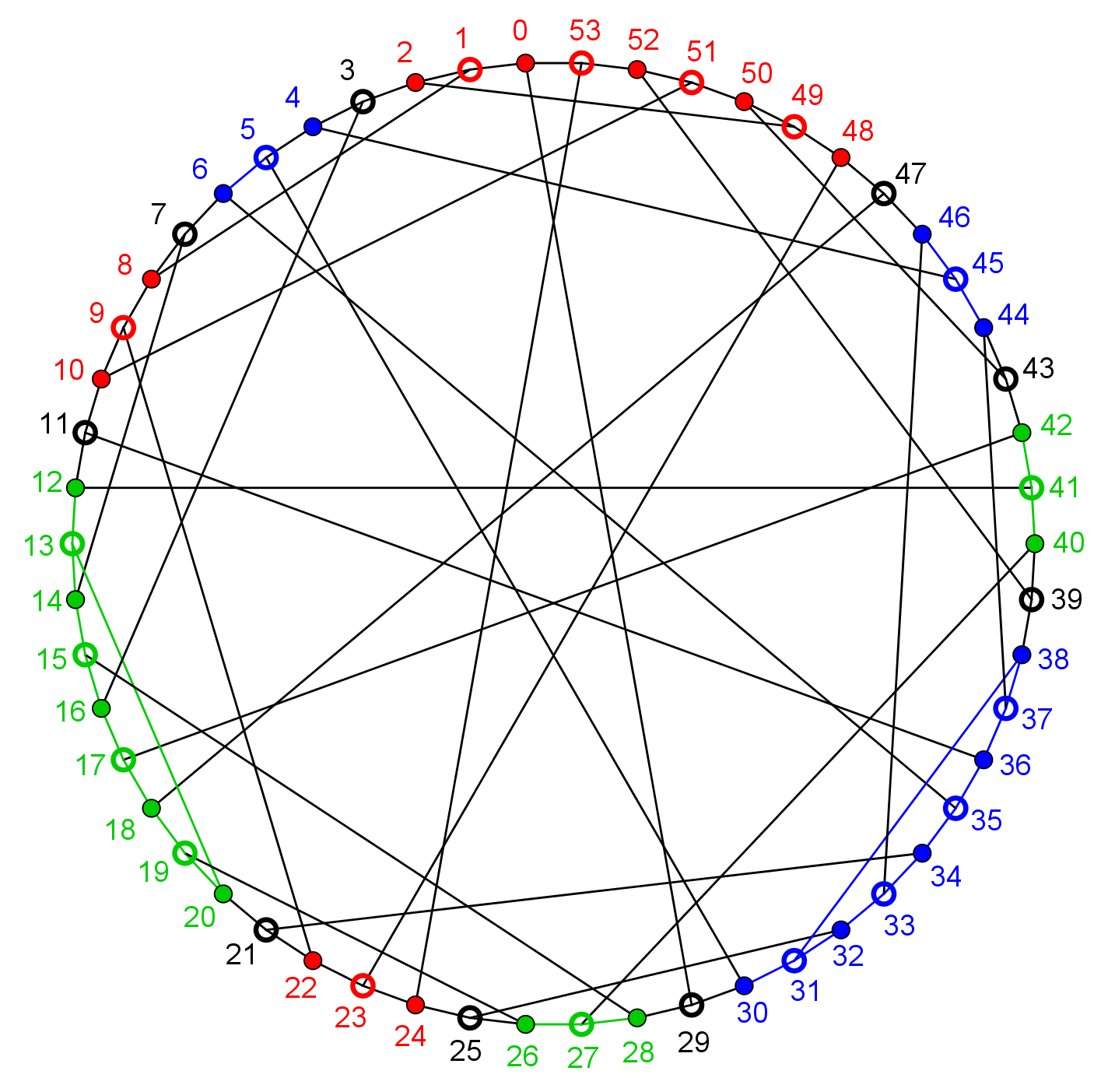
Figure 1: The Gray graph with standard vertex labeling, clearly displaying a Hamilton cycle and that it is bipartite, with the bipartition given by hollow and solid vertices. The colour code is explained in the text.

Clearly, the Hamilton cycle in Figure 1 is symmetric with respect to a cyclic group $\mathbb{Z}_{3}$, shown as 3-fold rotation, generated by

$$\varrho=(0,18,36)(1,19,37)\ldots(17,35,53).$$

The Gray graph is the Levi graph—that is, the point-line incidence graph—of the Gray configuration. This is a $(27_{3})$ configuration which occurs as a member of an infinite family of configurations defined by Bouwer in 1972 [2, Section 1]. Corresponding to this definition, it can be realized as a spatial configuration consisting of the 27 points and 27 lines of a $3\times 3\times 3$ integer grid (see Figure 2). It can be decomposed (in three different ways) into 3 grid-like $(9_{2},6_{3})$ subconfigurations lying in 3 parallel planes, and a pencil of 9 parallel lines which are perpendicular to these planes. In Figure 1 we distinguish the vertices representing the points (solid) and lines (hollow) of these subconfigurations by colouring red, green and blue, while the lines connecting these copies are represented by black hollow vertices. There is an automorphism of the Gray configuration which cyclically permutes these subconfigurations; in terms of the Gray graph, the transformation $\varrho$ corresponds just to this automorphism.

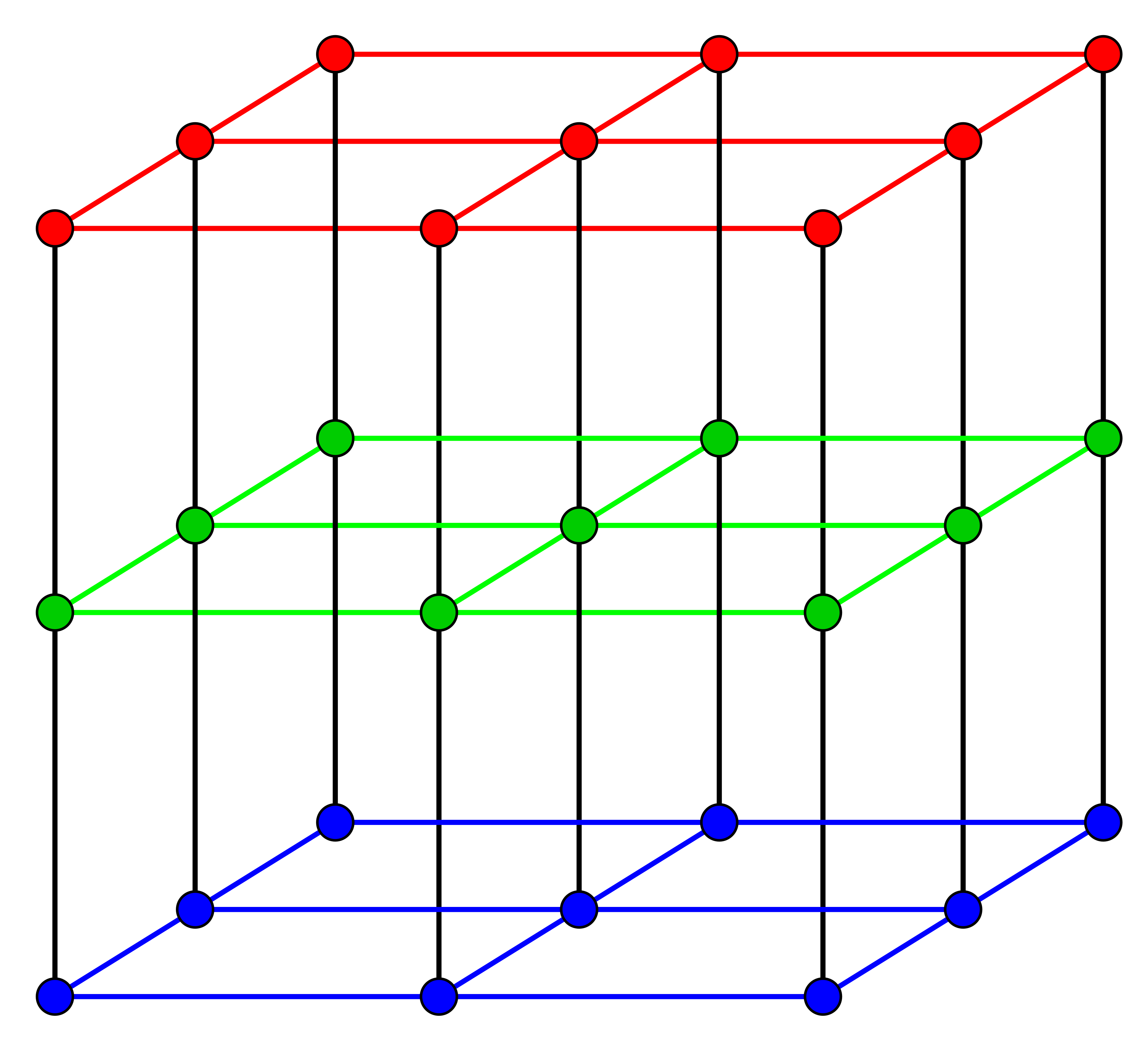
Figure 2: The Gray configuration: the standard spatial realization. Each coloured horizontal slice represents a $(9_{2},6_{3})$ subconfiguration.

2 A polycirculant unit-distance representations of the Gray graph

A drawing of a polycirculant graph $\Gamma$ with respect to some semi-regular automorphism $\pi\in\mathbb{Z}_{m}$ is polycirculant drawing if $\mathbb{Z}_{m}$ also acts semi-regularly on the geometric graph, where the edges are represented as line segments. Since a cyclic symmetry group in the plane acts as rotations, the vertices of the same orbit are equally spaced on a circle. If, in addition, all edge segments are of the same length, the drawing is a polycirculant unit-distance representation of $\Gamma$ in the Euclidean plane. There are many cases of polycirculant drawings in the past, although this is the first time we introduce this term formally. For instance, see [11] where unit-distance polycyclic drawings of generalized Petersen graphs are presented. Although generalized Petersen graphs and $I$-graphs are bicirculants (see e.g. [1]), some of them can be viewed as tetracirculants, such as the Nauru and ADAM graphs in [4].

In what follows we give a construction which proves that there exists a polycirculant unit-distance representation of the Gray graph with respect to the $\mathbb{Z}_{3}$ symmetry determined by $\varrho$. It has two degrees of freedom.

Construction 1.

1. Consider the Levi graph of the $(9_{2},6_{3})$ subconfiguration of the Gray configuration (see Figure 3a). Construct a polycirculant unit-distance representation of it (Figure 3b), e.g. in the following way. First arrange 6 hollow points so as to form the set of vertices of a regular hexagon. Then choose a radius $r$, and draw circles with this radius around each of the 6 points. By suitably pairing these circles, their points of intersection yield the desired solid points. Denote this representation by $G_{0}$. It has threefold rotational (in fact, dihedral) symmetry. In addition, it has one degree of freedom, the size of the radius $r$.

   

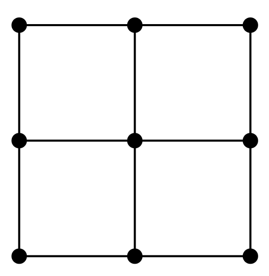
   (a)

   

   (b)

   Figure 3: (a) A $(9_{2},6_{3})$ subconfiguration of the Gray configuration; (b) $G_{0}$: a polycirculant unit-distance representation of the Levi graph of this subconfiguration.

2. Take a vector star which consists of three unit vectors that emanate from a common point whose endpoints coincide with the vertices of an equilateral triangle. Denote it by $S$.

3. Start from $G_{0}$, and form its three translated images using the vectors of $S$ as translation vectors. Denote these translates by $G_{b}$, $G_{g}$ and $G_{r}$. Note that the orientation of the vector star relative to $G_{0}$ determines a new, second degree of freedom of the construction; indeed, the mutual position of the three translates of $G_{0}$ changes when rotating the vector star (see Figure 4).

   

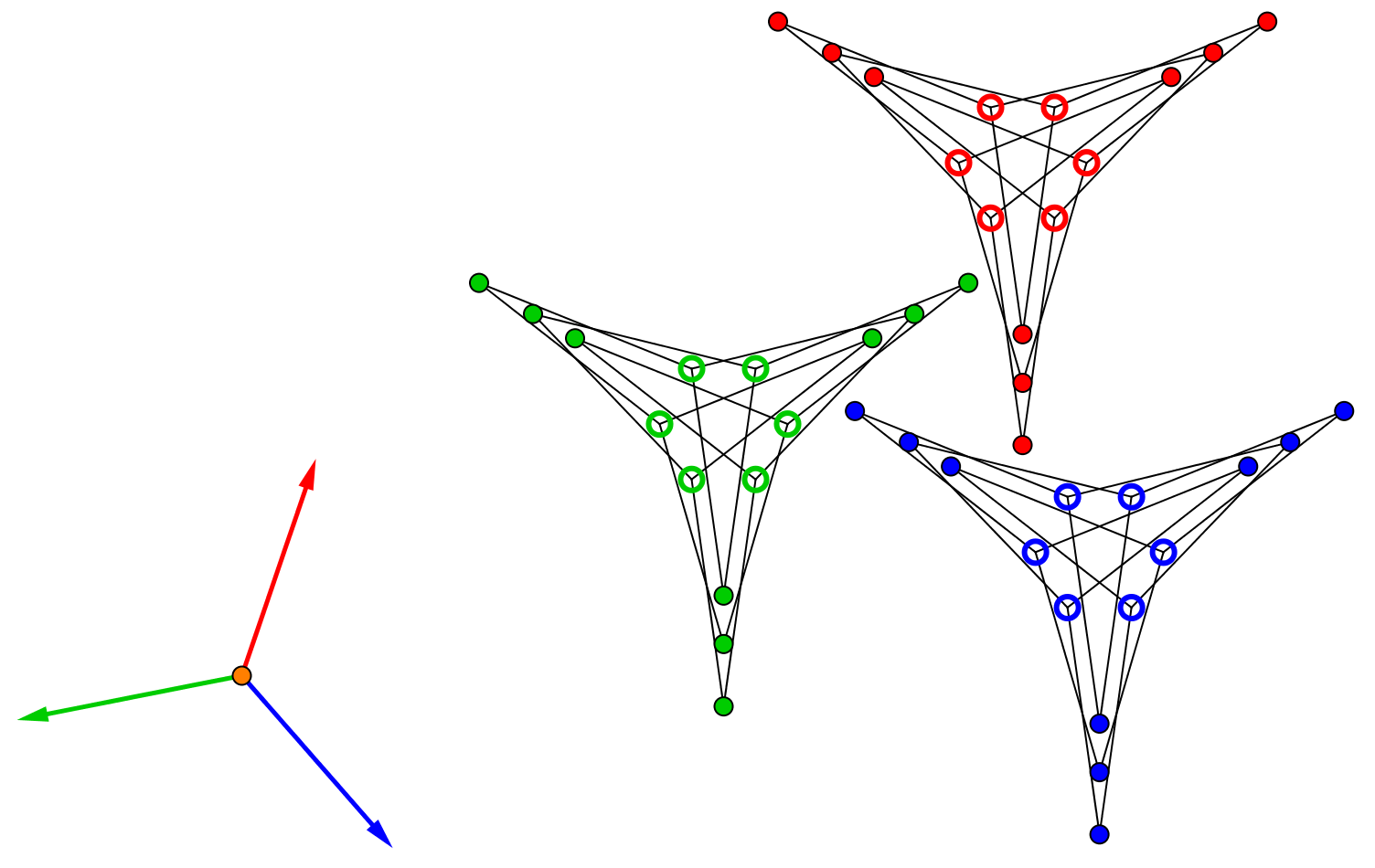
   Figure 4: Illustration for Step (3).

4. Take the set-union

   $$G_{b}\cup G_{g}\cup G_{r}\cup V_{p}(G_{0}),$$

   where $V_{p}(G_{0})$ denotes the set of vertices of $G_{0}$ representing the points of the $(9_{2},6_{3})$ configuration (thus these vertices are denoted by solid vertices). Denote the (disconnected) geometric graph obtained in this way by $U$.

5. In this graph $U$, switch the notation of the 9 points coming from $V_{p}(G_{0})$ from solid points to hollow points. Note that, at this stage, $U$ contains $3\times 9=27$ solid points and $(3\times 6)+9=27$ hollow points, plus 54 edges, coming only from the three subgraphs $G_{b}$, $G_{r}$, and $G_{b}$.

6. Observe that due to Step (3), in the vicinity of each of the 9 isolated vertices of $U$ there are precisely 3 solid points at a unit distance, one from each of $G_{b}$, $G_{g}$ and $G_{r}$. Make this graph connected by inserting $9\times 3$ new edges between the isolated vertices and their neighbours of valency 2. The resulting graph now has $54+27=81$ edges and $27$ solid points and $27$ hollow points.

The final unit-distance graph is shown in Figure 5. It is both polycirculant with $\mathbb{Z}_{3}$ rotational symmetry and unit-distance; in addition, it is isomorphic to the Gray graph. It has two degrees of freedom, as described in Steps (1) and (3), corresponding to a choice of unit distance and a choice of angle of rotation of the three coloured subgraphs with respect to the black hollow points.

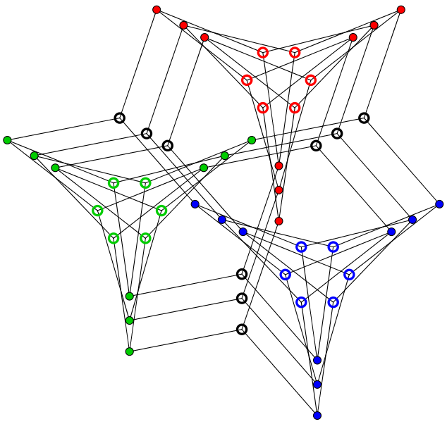
Figure 5: A polycirculant unit-distance representation of the Gray graph.

We note that there is a connection between unit-distance graphs and point-circle isometric configurations (here “isometric” means that all circles in such a configuration are of the same size; see, for instance [3]). In our particular case this means that drawing 27 unit circles centred at the hollow vertices of the Figure 5 forms, together with the solid vertices, an isometric point-circle realization of the Gray configuration.

Finally, we also note that there are certain similarities between drawing polycyclic configurations and their polycirculant Levi graphs.

References

- [1] Marko Boben, Tomaž Pisanski, and Arjana Žitnik. -graphs and the corresponding configurations. J. Combin. Des., 13(6):406–424, 2005.
- [2] Izak Zurk Bouwer. On edge but not vertex transitive regular graphs. J. Combin Theory Ser. B., 12:32–40, 1972.
- [3] Gábor Gévay and Tomaž Pisanski. Kronecker covers, -construction, unit-distance graphs and isometric point-circle configurations. Ars Math. Contemp., 7:317–336, 2014.
- [4] Dragan Marušič and Tomaž Pisanski. The ADAM graph and its configuration. The Art of Discrete and Applied Mathematics, 1(1):E1–01, 2018.
- [5] Dragan Marušič and Tomaž Pisanski. The Gray graph revisited. J. Graph Theory, 35:1–7, 2000.
- [6] Dragan Marušič, Tomaž Pisanski, and Steve Wilson. The genus of the GRAY graph is 7. Eur. J. Combin., 26:377–385, 2005.
- [7] Barry Monson, Tomaž Pisanski, Egon Schulte, and Asia Ivić Weiss. Semisymmetric graphs from polytopes. J. Combin Theory Ser. A., 114:421–435, 2007.
- [8] Tomaž Pisanski. Yet another look at the Gray graph. New Zealand J. Math., 36:85–92, 2007.
- [9] Tomaž Pisanski and Milan Randić. Bridges between geometry and graph theory. In C. A. Gorini, editor, Geometry at Work, pages 174–194. Math. Assoc. America, Washington, DC, 2000.
- [10] Tomaž Pisanski and Brigitte Servatius. Configurations from a Graphical Viewpoint. Birkhäuser Advanced Texts. Birkhäuser, New York, 2013.
- [11] Arjana Žitnik, Boris Horvat, and Tomaž Pisanski. All generalized Petersen graphs are unit-distance graphs. J. Korean Math. Soc., 49:475–491, 2012.