Benign Nonconvex Landscapes in Optimal and Robust Control, Part I: Global Optimality

Abstract

Direct policy search has achieved great empirical success in reinforcement learning. Many recent studies have revisited its theoretical foundation for continuous control, which reveals elegant nonconvex geometry in various benchmark problems, especially in fully observable state-feedback cases. This paper considers two fundamental optimal and robust control problems with partial observability: the Linear Quadratic Gaussian (LQG) control with stochastic noises, and $\mathcal{H}_{\infty}$ robust control with adversarial noises. In the policy space, the former problem is smooth but nonconvex, while the latter one is nonsmooth and nonconvex. We highlight some interesting and surprising “discontinuity” of LQG and $\mathcal{H}_{\infty}$ cost functions around the boundary of their domains. Despite the lack of convexity (and possibly smoothness), our main results show that for a class of non-degenerate policies, all Clarke stationary points are globally optimal and there is no spurious local minimum for both LQG and $\mathcal{H}_{\infty}$ control. Our proof techniques rely on a new and unified framework of Extended Convex Lifting (ECL), which reconciles the gap between nonconvex policy optimization and convex reformulations. This $\mathtt{ECL}$ framework is of independent interest, and we will discuss its details in Part II of this paper.

1 Introduction

Inspired by the empirical successes of reinforcement learning (RL) in various applications [1, 2, 3], policy optimization techniques have received renewed interest in the control of dynamical systems with continuous action spaces [4, 5]. Significant advances have been established in terms of understanding the theoretical properties of direct policy search on a range of benchmark control problems, including stabilization [6, 7], linear quadratic regulator (LQR) [8, 9, 10, 11], linear risk-sensitive control [12], linear quadratic Gaussian (LQG) control [13, 14, 15, 16], dynamic filtering [17, 18], and linear distributed control [19, 20]; see [5] for a recent survey.

All these control problems are known to be nonconvex in the policy space. In classical control theory, one typical approach to deal with the nonconvexity is to reparameterize the problem (e.g. via a suitable change of variables [21, 22, 23, 24, 25]) into a convex form for which efficient algorithms exist. Indeed, since the 1980s, convex reformulations or relaxations become very popular and almost universally accepted as solutions for optimal and robust control problems. It is now well-known that many optimal and robust control problems can be reformulated as convex programs, using the linear matrix inequalities (LMIs) techniques [21, 26, 27], or relaxed via the sums of squares [28, 29]. These techniques can provide rigorous stability and safety certificates in terms of matrix inequalities representing Lyapunov or dissipativity conditions. To achieve such certificates, these convex approaches typically rely on certain controller reparameterizations [21, 22, 23, 24, 25], which often require an explicit underlying system model and are thus model-based designs.

When system models are unknown, complex, or poorly parameterized, direct policy optimization is another viable option for controller synthesis. In fact, this approach can date back to the 1970s [30, 31, 32, 33]. In principle, policy optimization is conceptually simpler, computationally more flexible, and also more amenable to learning-based control (as evidenced by the aforementioned successes of RL), but it naturally leads to nonconvex optimization (as pointed out above) for which it is harder to derive theoretical guarantees or certificates. Fortunately, despite the nonconvexity, a series of recent findings highlighted above have revealed favorable optimization landscape properties in many benchmark control problems. For example, global convergence of model-free policy gradient methods has been established for both discrete-time [8] and continuous-time LQR [10] thanks to the gradient dominance property of the cost functions; the LQG cost function has no spurious stationary points that correspond to controllable and observable policies [13]. Beyond LQR and LQG, global or local convergence results of direct policy search have also been established for linear risk-sensitive control [12] and distributed control problems [19, 20]. Furthermore, the work [34] has established a global convergence result of direct policy search for state-feedback $\mathcal{H}_{\infty}$ control. For output-feedback $\mathcal{H}_{\infty}$ control, it has been revealed in [35] that there always exists a continuous path connecting any initial stabilizing controller to a globally optimal controller.

These developments have highlighted elegant nonconvex geometry in various benchmark problems, generating momentous excitements at the interface of control theory, RL, and nonconvex optimization. However, so far, most existing results have focused on control problems with full-state observation for which the globally optimal policies are static. The theoretical understanding of policy optimization for partially observed systems, where dynamic policies are needed, remains limited. The few notable exceptions [13, 14, 17, 15] only deal with linear quadratic (LQ) control with stochastic noises, where their cost functions are nonconvex but smooth over the feasible region. Another fundamental control paradigm, known as robust control, addresses the worst-case performance against uncertainties or adversarial noises [23]. In this case, the performance measure is the $\mathcal{H}_{\infty}$ norm of a certain closed-loop transfer function, which is known to be nonconvex and nonsmooth in the policy space [36, 37]. In this paper, we focus on the policy optimization perspective of output-feedback systems in the cases of both stochastic noises (i.e., LQG control) and adversarial noises (i.e., $\mathcal{H}_{\infty}$ robust control). In the spirit of [38], our results provide a unified treatment to these two classical optimal and robust control problems, shedding new light on their benign yet intricate nonconvex optimization landscapes.

1.1 Our contributions

In this paper, we study two fundamental control problems with partial observability: the LQG control with stochastic noises, and $\mathcal{H}_{\infty}$ robust control with adversarial noises, from a modern nonconvex optimization perspective. Despite the nonconvexity, our results characterize the global optimality of a large class of stationary points for both LQG and $\mathcal{H}_{\infty}$ optimization over dynamic policies. A key concept underpinning our results is the notion of non-degenerate dynamic policies, which requires a Lyapunov variable with a full-rank off-diagonal block to certify the corresponding $\mathcal{H}_{2}$ or $\mathcal{H}_{\infty}$ norm of the closed-loop system; the precise definition is given in Section 3. Our main contributions towards the benign nonconvex landscapes of LQG and $\mathcal{H}_{\infty}$ control are summarized as follows:

1. Smooth nonconvex landscape of LQG control. Despite being analytical over its domain, we reveal that the LQG cost has intricate “discontinuous” behavior around the boundary of its domain: the LQG costs can converge to a finite value when dynamic policies go to its boundary, while with the same limiting policy, the LQG costs can also diverge to infinity (Example 4.1). We prove that if the limiting policy corresponds to a controllable and observable controller, the corresponding LQG costs will always diverge to infinity irrespective of the sequence of dynamic policies (Theorem 4.1). Our main technical result shows that for the class of non-degenerate policies, any stationary points are globally optimal in LQG control, and there exist no spurious stationary points (Theorem 4.2). Notably, this result includes the existing characterization of minimality in [13] as a special case (Theorem 4.3). Therefore, all potentially spurious stationary points belong to the class of degenerate policies. For this aspect, we further identify a class of degenerate stationary points that are likely to be sub-optimal (Theorem 4.4).

2. Nonsmooth and nonconvex landscape of $\mathcal{H}_{\infty}$ robust control. One key difference compared to LQG control is that $\mathcal{H}_{\infty}$ robust control has a nonsmooth cost function (this fact is known and also expected due to the max operation over adversarial noises; see Example 5.1). The non-smoothness indeed complicates analysis machinery. However, not surprisingly in the spirit of [38] (or surprisingly), we show that many landscape properties of LQG control have nonsmooth counterparts in $\mathcal{H}_{\infty}$ control. This is mainly because $\mathcal{H}_{2}$ and $\mathcal{H}_{\infty}$ norms have similar LMI characterizations. Similar to the LQG case, the nonsmooth $\mathcal{H}_{\infty}$ cost function also exhibits intricate “discontinuous” behavior around its boundary (Examples 5.2 and 5.1). One good property of $\mathcal{H}_{\infty}$ cost is that it is locally Lipschitz and also subdifferentially regular in the sense of Clarke, enabling the use of Clarke subdifferential for nonsmooth analysis [39, 40] (see Section B.1 for a review). Our main result is that all Clarke stationary points in the set of non-degenerate policies are globally optimal for $\mathcal{H}_{\infty}$ robust control (Theorem 5.2), and thus the set of non-degenerate policies has no spurious stationary points. Finally, we also highlight a class of Clarke stationary points that is potentially degenerate and sub-optimal (Theorem 5.3).

Our main technical results are established using a new and unified framework of Extended Convex Lifting (ECL), which reconciles the gap between nonconvex policy optimization and convex reformulations. The remarkable (now classical) results in control theory reveal that many optimal and robust control problems admit “convex reformulations” in terms of LMIs, via a suitable change of variables (which often comes from Lyapunov theory) [26, 21, 41, 27, 42]. Under suitable settings, these changes of variables establish a differemorphism that connects nonconvex policy optimization with their convex reformulations, enabling convex analysis for nonconvex problems. The technical details are involved, and we postponed them to Part II of this paper.

1.2 Related work

We review some related literature in this section. The review below is not intended to be exhaustive, but rather to outline some of the closely related work. We refer interested to some excellent textbooks [23, 41] for classical results on optimal and robust control, the monographs [27, 42] for LMIs in control, and excellent surveys [5, 4] for recent advances on policy optimization in controls. The interested reader might also see [43, 44, 45] for statistical learning theory for LQ control.

Policy optimization for smooth LQ control.

As mentioned earlier, policy optimization has a long history dating back to the 1970s and is one of the main workhorses for modern RL. There has been a recent surging interest in applying direct policy search to control complex dynamic systems [4, 5]. One emphasis is to obtain theoretical guarantees in terms of optimality, robustness, and sample complexity. For the classical LQR problem, it has been revealed that the cost function is coercive and smooth over any sublevel set, and gradient dominated [8]. These properties are fundamental to establishing global convergence of direct policy search and their model-free extensions for solving LQR [9, 10, 11]. Similar favorable nonconvex properties of risk-sensitive state-feedback control are revealed in [12]. Other recent results include Markovian jump LQR [46], distributed LQR [20, 19, 11], and finite-horizon LQ control [47].

All of these studies considered static policies with full state observations, i.e., the policy’s output only utilizes the current state observation but no historical information. Control problems with partial output observations typically require dynamic policies, e.g, involving a suitable state estimator. The resulting optimization landscape becomes richer and yet much more complicated than LQR. Our prior work [13] has revealed favorable landscape properties: 1) the set of stabilizing full-order dynamic policies has at most two path-connected components that are identical in the frequency domain; 2) all stationary points corresponding to controllable and observable controllers in LQG control are globally optimal. However, there exist suboptimal saddle points in the LQG landscape [13, Examples 5 & 6], which never appear in state feedback LQR. A saddle-escaping algorithm has been proposed in [14]. A few other recent studies include [15, 17, 18, 16]. In [17], the global convergence of policy search over dynamic filters was proved for a simpler estimation problem.

Policy optimization for nonsmooth robust control.

Direct policy optimization techniques for $\mathcal{H}_{\infty}$ robust control have been extensively studied since the early 2000s [37, 36, 48, 49, 50]. It is known that the closed-loop $\mathcal{H}_{\infty}$ norm is nonsmooth and not always differentiable in the policy space [36]. Indeed, robust control problems were one of the early motivations and applications for nonsmooth optimization [37]. Some of the early nonsmooth optimization algorithms for robust control have been implemented as software packages — HIFOO [51] and HINFSTRUCT [52], which have seen successful applications in practice. However, none of these early studies address the global optimality of policy search for robust control. Global optimality guarantees only appear recently for state-feedback $\mathcal{H}_{\infty}$ control [34]: any Clarke stationary points are globally optimum; see [35, 53] for related discussions.

The recent studies [34, 35] utilize convex reparameterization in terms LMIs to analyze the nonconvex policy optimization, which is consistent with the strategies in [13, 10, 19] for smooth LQ control. This analysis idea via convex reformulations was also studied in [54] for static state feedback policies. A related framework, called DCL, was proposed in [17], to study the nonconvex properties of Kalman filter. Despite sharing a similar spirit of exploiting LMI-based parameterization, our framework of $\mathtt{ECL}$ applies to a wider range of problems than all these existing studies [34, 35, 13, 10, 19, 17] in the sense that $\mathtt{ECL}$ works for both smooth and nonsmooth control problems, while naturally differentiating degenerate and non-degenerate policies.

Benign nonconvex landscapes in machine learning problems

Some exciting nonconvex optimization results have recently emerged in machine learning literature, where the underlying geometrical properties (such as rotational [55, 56, 57] and discrete [58, 59] symmetries) enable identifying the local curvature of stationary points and thus contribute to global optimality of gradient-based methods [60, 61, 62]. Many of these favorable nonconvex properties have been studied in [63] under smooth parametrizations of nonconvex problems into convex forms. However, control problems naturally involve extra Lyapunov variables with a unique feature of similarity transformations, which is very different from machine learning problems. Accordingly, our main technical results are established using a new analysis framework of $\mathtt{ECL}$ accounting for Lyapunov variables and similarity transformations. We believe this $\mathtt{ECL}$ framework is of independent interest, and the details will be presented in Part II of this paper.

1.3 Paper outline

The rest of this paper is organized as follows. Section 2 presents the problem statements of nonconvex policy optimization for Linear Quadratic Gaussian (LQG) control and $\mathcal{H}_{\infty}$ robust control. In Section 3, we overview a few LMI characterizations for the LQG cost and $\mathcal{H}_{\infty}$ cost, and we also introduce a class of non-degenerate stabilizing controllers. We present our main results on the global optimality of smooth and nonconvex LQG control in Section 4 and on the global optimality of nonsmooth and nonconvex $\mathcal{H}_{\infty}$ robust control in Section 5. Some numerical experiments are reported in Section 6. We finally conclude the paper in Section 7. Many auxiliary results, additional discussions, and technical proofs are provided in Appendices A, B, C and D.

Notations.

We use lower and upper case letters (e.g. $x$ and $A$) to denote vectors and matrices, respectively. Lower and upper case boldface letters (e.g. $\mathbf{x}$ and $\mathbf{G}$) are used to denote signals and transfer matrices, respectively. The set of $k\times k$ real symmetric matrices is denoted by $\mathbb{S}^{k}$, and the determinant of a square matrix $M$ is denoted by $\det M$. We denote the set of $k\times k$ real invertible matrices by $\mathrm{GL}_{k}=\{T\in\mathbb{R}^{k\times k}\mid\det T\neq 0\}$. Given a matrix $M\in\mathbb{R}^{k_{1}\times k_{2}}$, $M^{{\mathsf{T}}}$ denotes the transpose of $M$, and $\|M\|_{F}$ denotes the Frobenius norm of $M$. For any $M_{1},M_{2}\in\mathbb{S}^{k}$, we use $M_{1}\prec(\preceq)M_{2}$ and $M_{2}\succ(\succeq)M_{1}$ to mean that $M_{2}-M_{1}$ is positive (semi)definite. We denote the set of real-rational proper stable transfer matrices as $\mathcal{RH}_{\infty}$. For simplicity, we omit the dimension of transfer matrices, which shall be clear in the context. Also, we use $I$ (resp. $0$) to denote the identity matrix (resp. zero matrix) of compatible dimensions.

2 Motivations and Problem Statement

In this section, we first overview the formulations of optimal control with stochastic noises and robust control with adversarial disturbances, then introduce their policy optimization forms, and finally present the problem statement of our work. Many results introduced in this section are standard in classical control theory, and we refer to the book [23] if we do not explicitly mention their sources.

2.1 System dynamics and disturbances

We consider a continuous-time linear time-invariant (LTI) dynamical system

$$\dot{x}(t) =Ax(t)+Bu(t)+B_{w}w(t),$$ (1)

$$y(t) =Cx(t)+D_{v}v(t),$$

where $x(t)\in\mathbb{R}^{n}$ is the vector of state variables, $u(t)\in\mathbb{R}^{m}$ the vector of control inputs, $y(t)\in\mathbb{R}^{p}$ the vector of measured outputs available for feedback, and $w(t)\in\mathbb{R}^{n},v(t)\in\mathbb{R}^{p}$ are the disturbances on the system process and measurement at time $t$. Here we introduce the matrices $B_{w}\in\mathbb{R}^{n\times n}$ and $D_{v}\in\mathbb{R}^{p\times p}$ for a unified treatment of LQG and $\mathcal{H}_{\infty}$ control problems that will be presented later. For notational simplicity, we will drop the argument $t$ when it is clear in the context. We consider the following performance signal

$$z(t)=\begin{bmatrix}Q^{1/2}\\ 0\end{bmatrix}x(t)+\begin{bmatrix}0\\ R^{1/2}\end{bmatrix}u(t),$$ (2)

where $Q\succeq 0$ and $R\succ 0$ are performance weight matrices. Throughout the paper, we also make the following standard assumption (see Appendix A for a review of related notions).

Assumption 1.

In 1, $(A,B)$ is controllable and $(C,A)$ is observable.

In this paper, we consider two different settings with regard to the disturbances $w(t)$ and $v(t)$, and they lead to the LQG optimal control problem and the $\mathcal{H}_{\infty}$ robust control problem.

LQG optimal control with stochastic noises.

When $w(t)$ and $v(t)$ are white Gaussian noises with identity intensity matrices, i.e., $\mathbb{E}[w(t)w(\tau)]=\delta(t-\tau)I_{n}$ and $\mathbb{E}[v(t)v(\tau)]=\delta(t-\tau)I_{p}$, we consider an averaged mean performance

$$\mathfrak{J}_{\mathtt{LQG}}\coloneqq\lim_{T\rightarrow+\infty}\mathbb{E}\!\left[\frac{1}{T}\int_{0}^{T}z(t)^{{\mathsf{T}}}z(t)\,dt\right]=\lim_{T\rightarrow+\infty}\mathbb{E}\!\left[\frac{1}{T}\int_{0}^{T}\left(x^{{\mathsf{T}}}Qx+u^{{\mathsf{T}}}Ru\right)dt\right].$$

The classical problem of linear quadratic Gaussian (LQG) optimal control is formulated as

$$\min_{u(t)} \mathfrak{J}_{\mathtt{LQG}}$$ (3)

subject to $$~{}\lx@cref{creftype~refnum}{eq:Dynamic},$$

where the input $u(t)$ is allowed to depend on all past observation $y(\tau)$ with $\tau\leq t$.

$\mathcal{H}_{\infty}$ robust control with adversarial disturbances.

When $w(t)$ and $v(t)$ are deterministic disturbances, we consider the worst-case performance in an adversarial setup. Assume that the system starts from a zero initial state $x(0)=0$. Let $\mathcal{L}_{2}^{k}[0,\infty)$ be the set of square-integrable (bounded energy) signals of dimension $k$, i.e.,

$$\mathcal{L}_{2}^{k}[0,\infty):=\left\{u:[0,+\infty)\rightarrow\mathbb{R}^{k}\left|\,\|u\|_{2}\coloneqq\left(\int_{0}^{\infty}u(t)^{{\mathsf{T}}}u(t)dt\right)^{1/2}<\infty\right.\right\},$$

Denote $d(t)=\begin{bmatrix}w(t)\\ v(t)\end{bmatrix}\in\mathbb{R}^{p+n}$, and consider the worst-case performance when the disturbance signal $d(t)$ has bounded energy less than or equal to $1$ i.e., $d\in\mathcal{L}_{2}^{p+n}[0,+\infty)$ with $\|d\|_{2}\leq 1$:

$$\mathfrak{J}_{\infty}:=\sup_{\|d\|_{2}\leq 1}\;\int_{0}^{\infty}z(t)^{{\mathsf{T}}}z(t)\,dt=\sup_{\|d\|_{2}\leq 1}\int_{0}^{\infty}\left(x^{{\mathsf{T}}}Qx+u^{{\mathsf{T}}}Ru\right)dt.$$

The $\mathcal{H}_{\infty}$ robust control problem is formulated as

$$\min_{u(t)} \mathfrak{J}_{\infty}$$ (4)

subject to $$~{}\lx@cref{creftype~refnum}{eq:Dynamic}\text{ and }x(0)=0,$$

where the input $u(t)$ is allowed to depend on all past observation $y(\tau)$ with $\tau\leq t$.

It can be shown that for both LQG optimal control and $\mathcal{H}_{\infty}$ robust control, the cost values $\mathfrak{J}_{\mathtt{LQG}}$ and $\mathfrak{J}_{\infty}$ depend on $B_{w}$ and $D_{v}$ only via $B_{w}B_{w}^{{\mathsf{T}}}$ and $D_{v}D_{v}^{{\mathsf{T}}}$. We therefore define the weight matrices $W\coloneqq B_{w}B_{w}^{{\mathsf{T}}},\,V\coloneqq D_{v}D_{v}^{{\mathsf{T}}},$ and assume $B_{w}=W^{1/2}$ and $D_{v}=V^{1/2}$ without loss of generality. We now state the following standard assumptions, which is the counterpart to Assumption 1.

Assumption 2.

In both LQG optimal control and $\mathcal{H}_{\infty}$ robust control, the weight matrices satisfy $Q\succeq 0,R\succ 0,W\succeq 0,V\succ 0$. Furthermore, $(A,W^{1/2})$ is controllable, and $(Q^{1/2},A)$ is observable.

2.2 Dynamic feedback policies

When the full state $x(t)$ cannot be directly observed, static feedback policies in which $u(t)$ only depends on the measurement $y(t)$ cannot achieve optimal values of the LQG cost or the $\mathcal{H}_{\infty}$ cost in general. On the other hand, we also do not need to consider general nonlinear policies with memory [64]. Indeed, it is known that the optimal values of both 3 and 4 can be achieved or approximated by employing linear dynamic feedback policies of the form

$$\dot{\xi}(t) =A_{{\mathsf{K}}}\xi(t)+B_{{\mathsf{K}}}y(t),$$ (5)

$$u(t) =C_{{\mathsf{K}}}\xi(t)+D_{{\mathsf{K}}}y(t),$$

where $\xi(t)\in\mathbb{R}^{q}$ is the internal state, and $A_{{\mathsf{K}}},B_{{\mathsf{K}}},C_{{\mathsf{K}}}$ and $D_{{\mathsf{K}}}$ are matrices of proper dimensions that specify the policy dynamics; see [23, Chaps 14 & 16] and also Section A.7 for a brief summary of relevant results. We parameterize dynamic feedback policies of the form 5 by

$${\mathsf{K}}=\begin{bmatrix}D_{\mathsf{K}}&C_{\mathsf{K}}\\ B_{\mathsf{K}}&A_{\mathsf{K}}\end{bmatrix}\in\mathbb{R}^{(m+q)\times(p+q)}.$$

Combining 5 with 1 via simple algebra leads to the closed-loop system

$$\frac{d}{dt}\begin{bmatrix}x\\ \xi\end{bmatrix} =A_{\mathrm{cl}}({\mathsf{K}})\begin{bmatrix}x\\ \xi\end{bmatrix}+B_{\mathrm{cl}}({\mathsf{K}})\begin{bmatrix}w\\ v\end{bmatrix},$$ (6a)

$$z =C_{\mathrm{cl}}({\mathsf{K}})\begin{bmatrix}x\\ \xi\end{bmatrix}+D_{\mathrm{cl}}({\mathsf{K}})\begin{bmatrix}w\\ v\end{bmatrix},$$

where we denote the closed-loop system matrices by

$$A_{\mathrm{cl}}({\mathsf{K}})\coloneqq \begin{bmatrix}A+BD_{\mathsf{K}}C&BC_{\mathsf{K}}\\ B_{\mathsf{K}}C&A_{\mathsf{K}}\end{bmatrix}, B_{\mathrm{cl}}({\mathsf{K}})\coloneqq \begin{bmatrix}W^{1/2}&BD_{{\mathsf{K}}}V^{1/2}\\ 0&B_{{\mathsf{K}}}V^{1/2}\end{bmatrix},$$ (6b)

$$C_{\mathrm{cl}}({\mathsf{K}})\coloneqq \begin{bmatrix}Q^{1/2}&0\\ R^{1/2}D_{{\mathsf{K}}}C&R^{1/2}C_{{\mathsf{K}}}\end{bmatrix}, D_{\mathrm{cl}}({\mathsf{K}})\coloneqq \begin{bmatrix}0&0\\ 0&R^{1/2}D_{{\mathsf{K}}}V^{1/2}\end{bmatrix}.$$

Then, the transfer matrix from the disturbance $d(t)=\begin{bmatrix}w(t)\\ v(t)\end{bmatrix}$ to the performance signal $z(t)$ becomes

$$\mathbf{T}_{{zd}}({\mathsf{K}},s)=C_{\mathrm{cl}}({\mathsf{K}})\left(sI-A_{\mathrm{cl}}({\mathsf{K}})\right)^{-1}B_{\mathrm{cl}}({\mathsf{K}})+D_{\mathrm{cl}}({\mathsf{K}}).$$ (7)

When the closed-loop system 6 is internally stable (see Section 2.3 for precise definitions), it is a standard result in control theory that the LQG cost $\mathfrak{J}_{\mathtt{LQG}}$ of the closed-loop system 6 is related to the $\mathcal{H}_{2}$ norm of the transfer matrix $\mathbf{T}_{zd}({\mathsf{K}},s)$ by

$$\mathfrak{J}_{\mathtt{LQG}}=\|\mathbf{T}_{zd}({\mathsf{K}},\cdot)\|_{\mathcal{H}_{2}}^{2}=\frac{1}{2\pi}\int_{-\infty}^{+\infty}\operatorname{tr}\!\left(\mathbf{T}_{zd}({\mathsf{K}},j\omega)^{{\mathsf{H}}}\,\mathbf{T}_{zd}({\mathsf{K}},j\omega)\right)d\omega,$$

while the $\mathcal{H}_{\infty}$ cost of the closed-loop system 6 is related to the $\mathcal{H}_{\infty}$ norm of $\mathbf{T}_{zd}({\mathsf{K}},s)$ by

$$\mathfrak{J}_{\infty}=\|\mathbf{T}_{zd}({\mathsf{K}},\cdot)\|_{\mathcal{H}_{\infty}}^{2}=\left(\sup_{\omega\in\mathbb{R}}\sigma_{\max}(\mathbf{T}_{zd}({\mathsf{K}},j\omega))\right)^{\!2},$$

where $\sigma_{\max}(\cdot)$ denotes the largest singular value. We note that when $\mathfrak{J}_{\infty}<+\infty$, the closed-loop LTI system 6 with $x(0)=0$ can be viewed as a linear mapping that maps any disturbance signal $d(t)\in\mathcal{L}_{2}^{p+n}[0,+\infty)$ to the performance signal $z(t)\in\mathcal{L}_{2}^{m+n}[0,+\infty)$, and $\sqrt{\mathfrak{J}_{\infty}}$ is exactly the $\mathcal{L}_{2}^{p+n}[0,+\infty)\to\mathcal{L}_{2}^{m+n}[0,+\infty)$ induced $\mathcal{H}_{\infty}$ norm of the closed-loop LTI system 6, as shown above.

We refer to the dimension $q\geq 0$ of the internal state variable $\xi$ as the order of the dynamic policy 5. A dynamic policy is called full-order if $q=n$ and is called reduced-order if $q<n$. Since the globally optimal LQG or $\mathcal{H}_{\infty}$ policy can be realized or approximated by a dynamic policy of order at most $n$ [23, Chaps 14 & 16] (also see Section A.7 for a review), it is unnecessary to consider dynamic policies with orders beyond $n$. We also note that, any dynamic policy ${\mathsf{K}}=\begin{bmatrix}D_{\mathsf{K}}&C_{\mathsf{K}}\\ B_{\mathsf{K}}&A_{\mathsf{K}}\end{bmatrix}$ of order $q<n$ can be augmented to full-order policies given by

$$\tilde{{\mathsf{K}}}_{c}=\left[\begin{array}[]{c:cc}D_{\mathsf{K}}&C_{{\mathsf{K}}}&0\\[2.0pt] \hdashline B_{{\mathsf{K}}}&A_{{\mathsf{K}}}&0\\ \tilde{B}&0&\Lambda\end{array}\right],\qquad\tilde{{\mathsf{K}}}_{o}=\left[\begin{array}[]{c:cc}D_{\mathsf{K}}&C_{{\mathsf{K}}}&\tilde{C}\\[2.0pt] \hdashline B_{{\mathsf{K}}}&A_{{\mathsf{K}}}&0\\ 0&0&\Lambda\end{array}\right]$$ (8)

where $\Lambda\in\mathbb{R}^{(n-q)\times(n-q)}$ is an arbitrary stable matrix, and $\tilde{B}\in\mathbb{R}^{(n-q)\times p}$ and $\tilde{C}\in\mathbb{R}^{m\times(n-q)}$ are arbitrary. It is clear that the augmented policies $\tilde{{\mathsf{K}}}_{c}$ and $\tilde{{\mathsf{K}}}_{o}$ satisfy $\mathbf{T}_{zd}(\tilde{{\mathsf{K}}}_{c},s)=\mathbf{T}_{zd}(\tilde{{\mathsf{K}}}_{o},s)=\mathbf{T}_{zd}({\mathsf{K}},s)$ and thus induce the same LQG cost and $\mathcal{H}_{\infty}$ cost as ${\mathsf{K}}$.

The dynamic policy 5 is said to be strictly proper, if there exists no direct feedback term from the measurement $y(t)$, i.e., $D_{{\mathsf{K}}}=0$. The LQG problem requires strictly proper dynamic policies, since the measurement $y(t)$ is corrupted by white Gaussian noise with infinite covariance, and the LQG cost $\mathfrak{J}_{\mathtt{LQG}}$ would be infinite if $D_{\mathsf{K}}\neq 0$.

2.3 Policy optimization over internally stabilizing policies

We now introduce an important notion of internal stability that stems from control theory. A dynamic feedback policy 5 is said to internally stabilize the plant 1 if the the closed-loop matrix $A_{\mathrm{cl}}({\mathsf{K}})$ is (Hurwitz) stable, i.e., the real parts of all its eigenvalues are strictly negative. We denote

$$\mathcal{C}_{q} \coloneqq\left\{\left.{\mathsf{K}}=\begin{bmatrix}D_{{\mathsf{K}}}&C_{{\mathsf{K}}}\\ B_{{\mathsf{K}}}&A_{{\mathsf{K}}}\end{bmatrix}\in\mathbb{R}^{(m+q)\times(p+q)}\,\right|A_{\mathrm{cl}}({\mathsf{K}})\text{ is stable}\right\},$$ (9a)

$$\mathcal{C}_{q,0} \coloneqq\left\{\left.{\mathsf{K}}=\begin{bmatrix}D_{{\mathsf{K}}}&C_{{\mathsf{K}}}\\ B_{{\mathsf{K}}}&A_{{\mathsf{K}}}\end{bmatrix}\in\mathcal{C}_{q}\,\right|D_{{\mathsf{K}}}=0_{m\times p}\right\}.$$ (9b)

In other words, $\mathcal{C}_{q}$ parameterizes the set of internally stabilizing policies, while $\mathcal{C}_{q,0}$ parameterizes the set of strictly proper internally stabilizing policies. It can be shown (see [13]) that $\mathcal{C}_{q}$ is an open subset of $\mathbb{R}^{(m+q)\times(p+q)}$, and $\mathcal{C}_{q,0}$ is an open subset of the vector space

$$\mathcal{V}_{q}\coloneqq\left\{\left.{\mathsf{K}}=\begin{bmatrix}D_{\mathsf{K}}&C_{\mathsf{K}}\\ B_{\mathsf{K}}&A_{\mathsf{K}}\end{bmatrix}\,\right|D_{\mathsf{K}}=0\right\}.$$

Moreover, classical control theory establishes the following properties of the sets $\mathcal{C}_{q}$ and $\mathcal{C}_{q,0}$:

1. Any dynamic policy in $\mathcal{C}_{q,0}$ (resp. $\mathcal{C}_{q}$) induces a finite LQG cost $\mathfrak{J}_{\mathtt{LQG}}$ (resp. a finite $\mathcal{H}_{\infty}$ cost $\mathfrak{J}_{\infty}$).

2. Any dynamic policy of order $q\leq n$ with a finite LQG cost $\mathfrak{J}_{\mathtt{LQG}}$ (resp. a finite $\mathcal{H}_{\infty}$ cost $\mathfrak{J}_{\infty}$), can be augmented to a policy in $\mathcal{C}_{n,0}$ (resp. a policy in $\mathcal{C}_{n}$) with the same LQG cost (resp. $\mathcal{H}_{\infty}$ cost).

3. For any reduced-order policy ${\mathsf{K}}$ and the associated augmented policies $\tilde{{\mathsf{K}}}_{c}$ and $\tilde{{\mathsf{K}}}_{o}$ in 8, ${\mathsf{K}}\in\mathcal{C}_{q}$ implies $\tilde{{\mathsf{K}}}_{c}\in\mathcal{C}_{n}\text{ and }\tilde{{\mathsf{K}}}_{o}\in\mathcal{C}_{n}$, and ${\mathsf{K}}\in\mathcal{C}_{q,0}$ implies $\tilde{{\mathsf{K}}}_{c}\in\mathcal{C}_{n,0}\text{ and }\tilde{{\mathsf{K}}}_{o}\in\mathcal{C}_{n,0}$.

Therefore, we will mainly consider dynamic policies in $\mathcal{C}_{n,0}$ (resp. $\mathcal{C}_{n}$) for the LQG optimal control (resp. the $\mathcal{H}_{\infty}$ robust control).

We are now ready to view LQG optimal control 3 and $\mathcal{H}_{\infty}$ robust control 4 from a modern perspective of policy optimization. Specifically, we will introduce cost functions $J_{\mathtt{LQG},q}:\mathcal{C}_{q,0}\rightarrow\mathbb{R}$ and $J_{\infty,q}:\mathcal{C}_{q}\rightarrow\mathbb{R}$, and formulate 3 and 4 as minimization of these cost functions.

LQG policy optimization.

Given $q\leq n$ and ${\mathsf{K}}\in\mathcal{C}_{q,0}$, we define

$$J_{\mathtt{LQG},q}({\mathsf{K}})=\|\mathbf{T}_{zd}({\mathsf{K}},\cdot)\|_{\mathcal{H}_{2}},$$ (10)

which is also equal to $\sqrt{\mathfrak{J}_{\mathtt{LQG}}}$ for the closed-loop system with the dynamic policy ${\mathsf{K}}$. It can be seen that $J_{\mathtt{LQG},q}$ gives a function defined over the domain $\mathcal{C}_{q,0}$ with values in $(0,+\infty)$. As a result, we can formulate the LQG optimal control 3 as the following policy optimization problem:

$$\min_{{\mathsf{K}}} J_{\mathtt{LQG},n}({\mathsf{K}})$$ (11)

subject to $${\mathsf{K}}\in\mathcal{C}_{n,0}.$$

Here we only consider optimizing over full-order dynamic policies in $\mathcal{C}_{n,0}$, since any reduced-order policy in $\mathcal{C}_{q,0}$ can be augmented to a full-order policy in $\mathcal{C}_{n,0}$ by (8) without changing the LQG cost. It can be shown that the set of full-order strictly proper internally stabilizing policies $\mathcal{C}_{n,0}$ is nonempty as long as Assumptions 1 and 2 hold; we refer to [13] for other geometrical properties such as path-connectedness of $\mathcal{C}_{n,0}$. We also define $J_{\mathtt{LQG},q}$ for $q\leq n$, which will be used for theoretical analysis.

It is known in classical control that $J_{\mathtt{LQG},q}({\mathsf{K}})$ can be computed by solving a Lyapunov equation, which is summarized in the lemma below [65, 31].

Lemma 2.1.

Fix $q\in\mathbb{N}$ such that $\mathcal{C}_{q,0}\neq\varnothing$. Given any ${\mathsf{K}}\in\mathcal{C}_{q,0}$, we have

$$J_{\mathtt{LQG},q}({\mathsf{K}})={} \sqrt{\operatorname{tr}\!\left(C_{\mathrm{cl}}({\mathsf{K}})X_{\mathsf{K}}C_{\mathrm{cl}}({\mathsf{K}})^{{\mathsf{T}}}\right)}=\sqrt{\operatorname{tr}\!\left(B_{\mathrm{cl}}({\mathsf{K}})^{{\mathsf{T}}}Y_{\mathsf{K}}B_{\mathrm{cl}}({\mathsf{K}})\right)},$$ (12)

where $X_{{\mathsf{K}}}$ and $Y_{{\mathsf{K}}}$ are the unique positive semidefinite solutions to the following Lyapunov equations

$$\begin{bmatrix}A&BC_{{\mathsf{K}}}\\ B_{{\mathsf{K}}}C&A_{{\mathsf{K}}}\end{bmatrix}X_{{\mathsf{K}}}+X_{{\mathsf{K}}}\begin{bmatrix}A&BC_{{\mathsf{K}}}\\ B_{{\mathsf{K}}}C&A_{{\mathsf{K}}}\end{bmatrix}^{{\mathsf{T}}}+\begin{bmatrix}W&0\\ 0&B_{{\mathsf{K}}}VB_{{\mathsf{K}}}^{{\mathsf{T}}}\end{bmatrix} =0,$$ (13a)

$$\begin{bmatrix}A&BC_{{\mathsf{K}}}\\ B_{{\mathsf{K}}}C&A_{{\mathsf{K}}}\end{bmatrix}^{{\mathsf{T}}}Y_{{\mathsf{K}}}+Y_{{\mathsf{K}}}\begin{bmatrix}A&BC_{{\mathsf{K}}}\\ B_{{\mathsf{K}}}C&A_{{\mathsf{K}}}\end{bmatrix}+\begin{bmatrix}Q&0\\ 0&C_{{\mathsf{K}}}^{{\mathsf{T}}}RC_{{\mathsf{K}}}\end{bmatrix} =0.$$ (13b)

$\mathcal{H}_{\infty}$ policy optimization.

Given $q\leq n$ and ${\mathsf{K}}\in\mathcal{C}_{q}$, we define

$$J_{\infty,q}({\mathsf{K}})=\|\mathbf{T}_{zd}({\mathsf{K}},\cdot)\|_{\mathcal{H}_{\infty}}=\sup_{\omega\in\mathbb{R}}\sigma_{\max}(\mathbf{T}_{zd}({\mathsf{K}},j\omega)),$$ (14)

which is also equal to $\sqrt{\mathfrak{J}_{\infty}}$ for the closed-loop system with the dynamic policy ${\mathsf{K}}$. We see that $J_{\infty,q}$ gives a function defined over $\mathcal{C}_{q}$ with values in $(0,+\infty)$. The $\mathcal{H}_{\infty}$ robust control 4 can then be reformulated into a policy optimization problem:

$$\min_{{\mathsf{K}}} J_{\infty,n}({\mathsf{K}})$$ (15)

subject to $${\mathsf{K}}\in{\mathcal{C}}_{n}.$$

where we only consider optimizing over $\mathcal{C}_{n}$ for similar arguments as in LQG policy optimization.

Instead of using the definition 14, there are state-space characterizations (e.g., the bounded real lemma in Lemma 3.2) for computing $J_{\infty,q}({\mathsf{K}})$ for ${\mathsf{K}}\in\mathcal{C}_{q}$. However, unlike the LQG cost that can be evaluated via solving Lyapunov equations 13, evaluating $J_{\infty,q}({\mathsf{K}})$ typically requires solving LMIs that admit no closed-form solutions. We also note that the classical $\mathcal{H}_{2}$ and $\mathcal{H}_{\infty}$ control often considers a general LTI system [23]; see Section A.6. It is straightforward to extend our main results to the general situation; see our conference report on $\mathcal{H}_{\infty}$ control [66].

2.4 Problem statements

The classical solutions for LQG control 3 and $\mathcal{H}_{\infty}$ robust control 4 explicitly depend on the system model $A,B,C$ in two different ways (see Theorems A.1 and A.2): one in formulating an observer-based controller, and another in solving Riccati equations to obtain feedback and observer gains. To avoid the explicit dependence on model parameters, we consider the policy optimization formulations 11 for LQG optimal control and 15 for $\mathcal{H}_{\infty}$ robust control, where the feedback policy is parameterized by ${\mathsf{K}}=(A_{\mathsf{K}},B_{\mathsf{K}},C_{\mathsf{K}},D_{\mathsf{K}})$ in 5. The idea of direct policy search is to start from an initial policy ${\mathsf{K}}_{0}\in\mathcal{C}_{n}$ and conduct the iteration ${\mathsf{K}}_{t+1}={\mathsf{K}}_{t}+\alpha_{t}F_{t},t\geq 0$, where $\alpha_{t}>0$ is a step size and $F_{t}$ is a search direction, such that the cost $J_{\mathtt{LQG},n}({\mathsf{K}})$ or $J_{\infty,n}({\mathsf{K}})$ is gradually improved. In addition to being more amenable to model-free control, it is observed that policy optimization is also more flexible as evidenced by the advances in modern reinforcement learning, and more scalable as it directly searches policies using computationally cheap iterates.

However, both policy optimization 11 and 15 are naturally nonconvex problems, making theoretical guarantees for direct policy search challenging. In this paper, we highlight some benign nonconvex landscape properties of policy optimization 11 and 15, which allow us to certify global optimality for a class of stationary points. In particular, we focus on the following two topics:

1. Smooth and nonconvex LQG control, which will be studied in Section 4. It is well-known that many linear quadratic control problems (including the LQG control $J_{\mathtt{LQG},q}({\mathsf{K}})$) are smooth and infinitely differentiable over their domains [19, 8, 46, 11]. Furthermore, many state-feedback cases (such as the standard LQR) have no spurious stationary points, and satisfy favorable coercivity and gradient dominance properties. However, landscape results for partially observed cases such as the LQG control are much fewer, with notable exceptions in [13, 14, 67]. As our first main contribution, we will reveal the hidden convexity in LQG policy optimization 11, and certify the global optimality for a class of stationary points (which we call non-degenerate policies).

2. Nonsmooth and nonconvex robust control, which will be studied in Section 5. Unlike LQR or LQG, it is known that the $\mathcal{H}_{\infty}$ cost is nonsmooth with respect to its argument due to two possible sources of non-smoothness: One from taking the largest singular of complex matrices, and the other from maximization over all the frequencies $\omega\in\mathbb{R}$. Direct policy search for $\mathcal{H}_{\infty}$ control has been used in earlier studies [36, 48, 49], but no optimality guarantees are given. Only very recently, a global optimality guarantee is given for state-feedback $\mathcal{H}_{\infty}$ control [34]. As our second main contribution, we will also reveal hidden convexity in nonsmooth $\mathcal{H}_{\infty}$ policy optimization 15, and show that for a class of non-degenerate policies, all Clarke stationary points in 15 are globally optimal.

To support our results for both LQG and $\mathcal{H}_{\infty}$ control, we will formally introduce a notion of non-degenerate stabilizing policies in Section 3. The proofs of our main global optimality characterizations rely on a new $\mathtt{ECL}$ framework which is the main topic of Part II of this paper.

3 Strict/Nonstrict LMIs and Non-degenerate Policies

In this section, we give an overview of LMI characterizations for both the LQG cost in 11 and $\mathcal{H}_{\infty}$ cost in 15, which play a key role in our analysis based on convex reformulations [21, 42]. We will also highlight some subtleties between strict and nonstrict LMIs, which motivate our definition of a general class of non-degenerate policies.

3.1 LMIs for smooth LQG cost and nonsmooth $\mathcal{H}_{\infty}$ cost

As shown in 10, the LQG cost for a strictly proper stabilizing policy ${\mathsf{K}}\in{\mathcal{C}}_{q,0}$ can be characterized by the $\mathcal{H}_{2}$ norm of the transfer function $\mathbf{T}_{zd}({\mathsf{K}},s)$. Although the $\mathcal{H}_{2}$ (and $\mathcal{H}_{\infty}$) norm of a stable transfer function can, in principle, be computed from their definitions, we here summarize some alternative characterizations, involving Lyapunov equations and LMIs.

Lemma 3.1.

Consider a transfer function $\mathbf{G}(s)=C(sI-A)^{-1}B$, where $A\in\mathbb{R}^{n\times n}$ is stable and $C\in\mathbb{R}^{p\times n},B\in\mathbb{R}^{n\times m}$. The following statements hold.

1. (Lyapunov equations). We have $\|\mathbf{G}\|_{\mathcal{H}_{2}}^{2}=\mathrm{trace}(B^{{\mathsf{T}}}L_{\mathrm{o}}B)=\mathrm{trace}(CL_{\mathrm{c}}C^{{\mathsf{T}}})$, where $L_{\mathrm{o}}$ and $L_{\mathrm{c}}$ are observability and controllability Gramians which can be obtained from the Lyapunov equations

   $$AL_{\mathrm{c}}+L_{\mathrm{c}}A^{{\mathsf{T}}}+BB^{{\mathsf{T}}} =0,$$ (16a)

   $$A^{{\mathsf{T}}}L_{\mathrm{o}}+L_{\mathrm{o}}A+C^{{\mathsf{T}}}C =0.$$ (16b)

2. (Strict LMI). $\|\mathbf{G}\|_{\mathcal{H}_{2}}<\gamma$ if and only if there exist $P\in\mathbb{S}^{n}_{++}$ and $\Gamma\in\mathbb{S}^{p}_{++}$such that the following strict LMI is feasible:

   $$\begin{bmatrix}A^{{\mathsf{T}}}P+PA&PB\\ B^{{\mathsf{T}}}P&-\gamma I\end{bmatrix} \prec 0,\;\;\begin{bmatrix}P&C^{{\mathsf{T}}}\\ C&\Gamma\end{bmatrix}\succ 0,\;\;\mathrm{trace}(\Gamma)<\gamma.$$ (17)

3. (Nonstrict LMI). $\|\mathbf{G}\|_{\mathcal{H}_{2}}\leq\gamma$ if there exist $P\in\mathbb{S}^{n}_{++}$ and $\Gamma\in\mathbb{S}^{p}_{+}$ such that the following nonstrict LMI is feasible:

   $$\begin{bmatrix}A^{{\mathsf{T}}}P+PA&PB\\ B^{{\mathsf{T}}}P&-\gamma I\end{bmatrix} \preceq 0,\;\;\begin{bmatrix}P&C^{{\mathsf{T}}}\\ C&\Gamma\end{bmatrix}\succeq 0,\;\;\mathrm{trace}(\Gamma)\leq\gamma.$$ (18)

   The converse holds if $(A,B)$ is controllable.

It is clear that Lemma 2.1 can be considered as a direct application of the first result in Lemma 3.1. This lemma is classical in control [23, 42, 41]. To clarify some subtleties between strict and nonstrict LMIs 17 - 18, we reproduce a short proof of Lemma 3.1 in Section A.3. The proof in Section A.3 is constructive, i.e., we shall explicitly construct solutions satisfying 17 and 18 from the solution to 16. While the solution to 16 is unique, the solutions to 17 are not unique given any $\gamma>\|\mathbf{G}\|_{\mathcal{H}_{2}}$. Indeed, the solution set to 17 is convex and open; any sufficiently small perturbation to a feasible point remains feasible. This perturbation perspective, while somewhat less explicitly stated in the literature, is one crucial step in many synthesis tasks using strict LMIs (see, e.g., [21, 41]). Meanwhile, although not obvious, the solution set to the non-strict LMI 18 is in general not a singleton even when setting $\gamma=\|\mathbf{G}\|_{\mathcal{H}_{2}}$ (see Example A.1). If the system $(C,A)$ is also observable, then the solution to 18 is unique when setting $\gamma=\|\mathbf{G}\|_{\mathcal{H}_{2}}$ (see Lemma A.9).

We next present the celebrated bounded real lemma that gives a state-space characterization for the $\mathcal{H}_{\infty}$ norm of a stable transfer function using LMIs.

Lemma 3.2 (Bounded real lemma).

Consider $\mathbf{G}(s)=C(sI-A)^{-1}B+D$, where $A\in\mathbb{R}^{n\times n}$ is stable and $C\in\mathbb{R}^{p\times n},B\in\mathbb{R}^{n\times m},D\in\mathbb{R}^{p\times m}$. Let $\gamma>0$ be arbitrary. The following statements hold.

1. (Strict version, [41, Lemma 7.3]) $\|\mathbf{G}\|_{\mathcal{H}_{\infty}}<\gamma$ if and only if there exists a symmetric matrix $P$ such that

   $$\begin{bmatrix}A^{{\mathsf{T}}}P+PA&PB&C^{{\mathsf{T}}}\\ B^{{\mathsf{T}}}P&-\gamma I&D^{{\mathsf{T}}}\\ C&D&-\gamma I\end{bmatrix}\prec 0.$$ (19)

2. (Nonstrict version, [27, Section 2.7.3]) $\|\mathbf{G}\|_{\mathcal{H}_{\infty}}\leq\gamma$ if there exists a symmetric matrix $P$ such that

   $$\begin{bmatrix}A^{{\mathsf{T}}}P+PA&PB&C^{{\mathsf{T}}}\\ B^{{\mathsf{T}}}P&-\gamma I&D^{{\mathsf{T}}}\\ C&D&-\gamma I\end{bmatrix}\preceq 0.$$ (20)

   The converse holds if $(A,B)$ is controllable.

A more complete list of the strict version of Lemma 3.2 is summarized in [68, Corollary 12.3]. This lemma is also classical in control, and one general version – the Kalman-Yakubovich-Popov (KYP) lemma is arguably one of the most fundamental tools in systems theory [23, 42, 41]. The sufficiency of LMIs 19 and 20 is relatively easy to prove, which involves a control-theoretic interpretation of the variable $P$ to construct a storage function $V(x)=x^{{\mathsf{T}}}Px$ certifying a dissipativity condition. The necessity of LMIs 19 and 20 is more involved to prove. In Section A.3, we adopt convex duality techniques in [69, 70, 71] to highlight some subtleties between strict and non-strict LMIs.

3.2 Non-degenerate policies

We can use the LMI characterizations in Lemma 3.1 and 3.2 to formulate nonconvex (bilinear) matrix inequalities when fixing the full-order dynamic policies for $\mathcal{H}_{2}$ and $\mathcal{H}_{\infty}$ synthesis. It was realized in the early 1990s that those nonconvex matrix inequalities can be convexified using a sophisticated change of variables (see, for example, [42, 26] and the references therein). It is also possible to derive classical Riccatti inequalities from those matrix inequalities [72]. All the previous studies [42, 26] only use the strict LMIs 17 and 19. As we will see in Part II, strict LMIs can only characterize strict epigraphs of $J_{\mathtt{LQG},n}({\mathsf{K}})$ or $J_{\infty,n}({\mathsf{K}})$, but fail to characterize global optimality directly.

In this work, we aim to analyze the LQG and $\mathcal{H}_{\infty}$ cost functions instead of their upper bounds, and thus our subsequent results require non-strict LMIs 18 and 20. However, the non-strict LMIs 18 and 20 do not present sufficient and necessary conditions for $\mathcal{H}_{2}$ and $\mathcal{H}_{\infty}$ characterizations. This fact will affect our analysis framework based on $\mathtt{ECL}$ that will be formally introduced in Part II of our paper. This subsection introduces a broad class of non-degenerate policies that are closely related to the nonstrict LMIs 18 and 20. We also present their physical interpretations.

LQG optimal control

The nonstrict LMI in Lemma 3.1 is in general not equivalent to, but only provides a sufficient condition for $\|\mathbf{G}\|_{\mathcal{H}_{2}}\leq\gamma$ when $A$ is stable. Consequently, given ${\mathsf{K}}\in\mathcal{C}_{n,0}$ and $\gamma>0$, it is only a sufficient condition for $J_{\mathtt{LQG},n}({\mathsf{K}})\leq\gamma$ that there exist matrices $P$ and $\Gamma$ satisfying the followng matrix inequalities:

$$\begin{bmatrix}A_{\mathrm{cl}}({\mathsf{K}})^{{\mathsf{T}}}P+PA_{\mathrm{cl}}({\mathsf{K}})&PB_{\mathrm{cl}}({\mathsf{K}})\\ B_{\mathrm{cl}}({\mathsf{K}})^{{\mathsf{T}}}P&-\gamma I\end{bmatrix}\preceq 0,$$ (21a)

$$\begin{bmatrix}P&C_{\mathrm{cl}}({\mathsf{K}})^{{\mathsf{T}}}\\ C_{\mathrm{cl}}({\mathsf{K}})&\Gamma\end{bmatrix}\succeq 0,\;{P\succ 0},\;\mathrm{trace}(\Gamma)\leq\gamma,$$ (21b)

where $A_{\mathrm{cl}}({\mathsf{K}}),B_{\mathrm{cl}}({\mathsf{K}}),C_{\mathrm{cl}}({\mathsf{K}})$ are the closed-loop matrices of the policy ${\mathsf{K}}$, defined in 7. We are particularly interested in those policies ${\mathsf{K}}\in\mathcal{C}_{n,0}$ for which (21) can be satisfied with $\gamma=J_{\mathtt{LQG},n}({\mathsf{K}})$, as these values of $J_{\mathtt{LQG},n}({\mathsf{K}})$ can then be directly characterized by (21), which would further allow us to utilize convex reformulations of optimal control problems for the analysis of $J_{\mathtt{LQG},n}({\mathsf{K}})$.

Note that the Lyapunov variable $P$ in 21 is of dimension $2n\times 2n$. Upon partitioning

$$P=\begin{bmatrix}P_{11}&P_{12}\\ P_{12}^{{\mathsf{T}}}&P_{22}\end{bmatrix}\in\mathbb{S}^{2n}_{++},$$ (22)

we will see later that the invertibility of $P_{12}$ plays an important role in “convexifying” the bilinear matrix inequalities 21. Motivated by these observations, we define a class of non-degenerate policies that admit a Lyapunov variable $P\in\mathbb{S}^{2n}_{++}$ with an off-diagonal block $P_{12}$ having full rank to certify its LQG cost.

Definition 3.1.

A full-order dynamic policy ${\mathsf{K}}\in{\mathcal{C}}_{n,0}$ is called non-degenerate for LQG if there exists a $P\in\mathbb{S}^{2n}_{++}$ with $P_{12}\in\mathrm{GL}_{n}$ such that 21b and 21a hold with $\gamma=J_{\mathtt{LQG},n}({\mathsf{K}})$.

Precisely, we define the set of non-degenerate policies for LQG as

$${\mathcal{C}}_{\mathrm{nd},0}:=\left\{{\mathsf{K}}=\begin{bmatrix}D_{{\mathsf{K}}}&C_{{\mathsf{K}}}\\ B_{{\mathsf{K}}}&A_{{\mathsf{K}}}\end{bmatrix}\in{\mathcal{C}}_{n,0}\left|\begin{aligned} &\;\;\exists P\in\mathbb{S}^{2n}_{++}\;\mathrm{with}\;P_{12}\in\mathrm{GL}_{n},\;\Gamma\;\mathrm{such~{}that}\\ &\;\lx@cref{creftypecap~refnum}{eq:LQG-Bilinear-a}\;\mathrm{and}\;\lx@cref{creftypecap~refnum}{eq:LQG-Bilinear-b}\;\textrm{hold with}\;\gamma=J_{\mathtt{LQG},n}({\mathsf{K}})\end{aligned}\right.\right\}.$$ (23)

Non-degeneracy of dynamic policies for LQG has a nice physical interpretation. Given ${\mathsf{K}}\in{\mathcal{C}}_{n,0}$, it can be shown that the system and policy state variables $(x(t),\xi(t))$ follow a Gaussian process with mean and covariance

$$\lim_{t\rightarrow\infty}\mathbb{E}\left(\begin{bmatrix}x(t)\\ \xi(t)\end{bmatrix}\right)=0,\quad X_{{\mathsf{K}}}=\begin{bmatrix}X_{{\mathsf{K}},11}&X_{{\mathsf{K}},12}\\ X_{{\mathsf{K}},12}^{{\mathsf{T}}}&X_{{\mathsf{K}},22}\end{bmatrix}:=\lim_{t\rightarrow\infty}\mathbb{E}\left(\begin{bmatrix}x(t)\\ \xi(t)\end{bmatrix}\begin{bmatrix}x(t)\\ \xi(t)\end{bmatrix}^{{\mathsf{T}}}\right),$$ (24)

where $X_{{\mathsf{K}}}$ is the unique positive semidefinite solution to the Lyapunov equation 13a; see Section A.4 for a proof. Following the terminology in [17] (which only focuses on Kalman filtering), we say a policy ${\mathsf{K}}\in\mathcal{C}_{n,0}$ is informative if the steady-state correlation matrix $X_{{\mathsf{K}},12}:=\lim_{t\to\infty}\mathbb{E}\left(x(t)\xi^{{\mathsf{T}}}(t)\right)$ has full rank. Our next result shows that a policy in ${\mathcal{C}}_{n,0}$ is non-degenerate for LQG if and only if it is informative.

Theorem 3.1.

Given ${\mathsf{K}}\in{\mathcal{C}}_{n,0}$, we have ${\mathsf{K}}\in{\mathcal{C}}_{\mathrm{nd},0}$ if and only if ${\mathsf{K}}$ is informative in the sense that

$$X_{{\mathsf{K}},12}:=\lim_{t\to\infty}\mathbb{E}\left(x(t)\xi^{{\mathsf{T}}}(t)\right)$$

has full rank.

The sufficiency part of Theorem 3.1 can be proved by the following idea: We first show that the full rank of $X_{{\mathsf{K}},12}$ leads to the controllability of $(A_{\mathsf{K}},B_{{\mathsf{K}}})$, which further implies that $X_{{\mathsf{K}}}$ from 13a is positive definite (cf. [13, Lemma 4.5]). As a result, $P=\gamma X_{{\mathsf{K}}}^{-1}$ with $\gamma=J_{\mathtt{LQG},n}({\mathsf{K}})$ is well-defined and we can show it satisfies 21a and 21b. Further, $P_{12}=\gamma(X_{{\mathsf{K}}}^{-1})_{12}$ is invertible since $X_{{\mathsf{K}},12}$ is, which completes the proof of sufficiency. The necessity part is more technically involved, and we provide all the proof details in Section D.2.

We can further show that non-degenerate policies are “generic” in the sense that the complement set ${\mathcal{C}}_{n,0}\backslash{\mathcal{C}}_{\mathrm{nd},0}$ has measure zero. The proof relies on the fact that the zero-set of a nontrivial real-analytic function has measure zero (cf. [73]). The details are technical, and we postpone them to Section D.3.

Theorem 3.2.

The set difference ${\mathcal{C}}_{n,0}\backslash{\mathcal{C}}_{\mathrm{nd},0}$ has measure zero.

The following example provides numerical evidence illustrating that ${\mathcal{C}}_{n,0}\backslash{\mathcal{C}}_{\mathrm{nd},0}$ has measure zero.

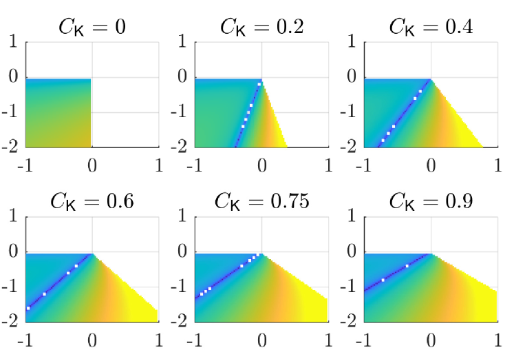
(a) LQG case in Example 3.1

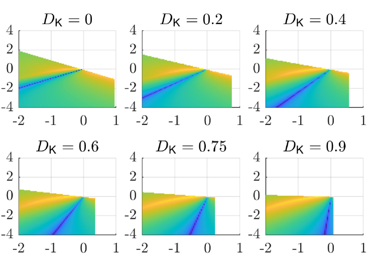
(b) $\mathcal{H}_{\infty}$ case in Example 3.2

Figure 1: Illustration that the set of degenerate policies has measure zero. (a) The case of LQG control 23: Heatmaps of $\ln|P_{12}|$ for different values of $C_{\mathsf{K}}$. (b) The case of $\mathcal{H}_{\infty}$ control 26: Heatmaps of $\ln|P_{12}|$ for different values of $D_{\mathsf{K}}$. In both subfigures, the $x$-axes and $y$-axes represent $A_{{\mathsf{K}}}$ and $B_{{\mathsf{K}}}$ respectively. Points with very low values of $\ln|P_{12}|$ (i.e., points whose corresponding $P_{12}$ are very close to $0$) are colored in dark blue, and they roughly form a line passing through $(0,0)$ in each sub-figure which has measure zero.

Example 3.1 (${\mathcal{C}}_{n,0}\backslash{\mathcal{C}}_{\mathrm{nd},0}$ has measure zero).

Consider an open-loop stable dynamic system 1 with $A=-1,\;B=1,\;C=1.$ We choose $Q=R=1,W=V=1$ for the LQG in 11. Our task is to numerically search for points in ${\mathcal{C}}_{n,0}\backslash{\mathcal{C}}_{\mathrm{nd},0}$, and inspect whether they form a set of measure zero. We imposes the constraints $A_{\mathsf{K}}\in[-1,1],B_{\mathsf{K}}\in[-2,2]$. We first generate a set of points $\{{\mathsf{K}}_{j}\}_{j=1}^{N}$ by discretizing the region $[-1,1]\times[-2,2]$ into a spacial grid with $N=101\times 101$ points that are equally spaced. Then for each $j=1,\ldots,N,$ we numerically compute $\gamma_{j}=J_{\mathtt{LQG},1}({\mathsf{K}}_{j})$ and try to construct $P_{j}\succeq 0$ by solving a Lyapunov equation (cf. Theorem 3.1). We then check whether the smallest eigenvalue of $P_{j}$ is sufficiently bounded away from zero (say greater than or equal to $10^{-5}$), and record the value of $(P_{j})_{12}$. Figure 1(a) illustrates several heatmaps of $\ln|P_{12}|$ with fixed $C_{\mathsf{K}}$ and varying $(A_{\mathsf{K}},B_{\mathsf{K}})$, generated from the recorded values of $\{\ln|(P_{j})_{12}|\}_{j=1}^{N}$. Points with low values of $\ln|P_{12}|$ (i.e., points whose corresponding $P_{12}$ are close to $0$) are colored in dark blue, and we observe that they roughly form a line passing through $(0,0)$ in each sub-figure, which has measure zero. ∎

$\mathcal{H}_{\infty}$ robust control

Similar to the LQG case, for the $\mathcal{H}_{\infty}$ policy optimization problem 15, we focus on the policies ${\mathsf{K}}\in\mathcal{C}_{n}$ such that the following set of matrix inequalities are satisfied by some matrix $P$ with $\gamma=J_{\infty,n}({\mathsf{K}})$:

$$\begin{bmatrix}A_{\mathrm{cl}}({\mathsf{K}})^{{\mathsf{T}}}P+PA_{\mathrm{cl}}({\mathsf{K}})&PB_{\mathrm{cl}}({\mathsf{K}})&C_{\mathrm{cl}}({\mathsf{K}})^{{\mathsf{T}}}\\ B_{\mathrm{cl}}({\mathsf{K}})^{{\mathsf{T}}}P&-\gamma I&D_{\mathrm{cl}}({\mathsf{K}})^{{\mathsf{T}}}\\ C_{\mathrm{cl}}({\mathsf{K}})&D_{\mathrm{cl}}({\mathsf{K}})&-\gamma I\end{bmatrix}\preceq 0,$$ (25a)

$${P\in\mathbb{S}^{2n}_{++}},$$ (25b)

where $A_{\mathrm{cl}}({\mathsf{K}}),B_{\mathrm{cl}}({\mathsf{K}}),C_{\mathrm{cl}}({\mathsf{K}})$ and $D_{\mathrm{cl}}({\mathsf{K}})$ are the closed-loop matrices for policy ${\mathsf{K}}$, defined in 7. The matrix $P$ has a dimension of $2n$-by-$2n$ and can be partitioned as 22.

Similar to Section 3.1, the invertibility of $P_{12}$ plays an important role in “convex reformulations” of 25. We thus define a class of non-degenerate policies for $\mathcal{H}_{\infty}$ control, which admits a Lyapunov variable $P\in\mathbb{S}^{2n}_{++}$ with an off-diagonal block $P_{12}$ having full rank to certify its $\mathcal{H}_{\infty}$ cost.

Definition 3.2.

A full-order dynamic policy ${\mathsf{K}}\in{\mathcal{C}}_{n}$ is called non-degenerate for $\mathcal{H}_{\infty}$ control if there exists a $P\in\mathbb{S}^{2n}_{++}$ with $P_{12}\in\mathrm{GL}_{n}$ such that 25a holds with $\gamma=J_{\infty,n}({\mathsf{K}})$.

We thus define the set of non-degenerate policies for $\mathcal{H}_{\infty}$ control as

$${\mathcal{C}}_{\mathrm{nd}}:=\left\{{\mathsf{K}}=\begin{bmatrix}D_{{\mathsf{K}}}&C_{{\mathsf{K}}}\\ B_{{\mathsf{K}}}&A_{{\mathsf{K}}}\end{bmatrix}\in\mathcal{C}_{n}\left|\begin{aligned} \;\;\exists P&\in\mathbb{S}^{2n}_{++}\;\mathrm{with}\;P_{12}\in\mathrm{GL}_{n}\;\\ \;\mathrm{such~{}that}\;&\lx@cref{creftypecap~refnum}{eq:Hinf-Bilinear-a}\;\textrm{holds with}\;\gamma=J_{\infty,n}({\mathsf{K}})\end{aligned}\right.\right\}.$$ (26)

We conjecture that non-degenerate policies are “generic” in the sense that the complement set $\mathcal{C}_{n}\backslash\mathcal{C}_{\mathrm{nd}}$ has measure zero. Unlike the smooth LQG case, a rigorous proof of this conjecture seems challenging, and we leave it to future work. One main difficulty for the proof lies in the non-smoothness of the $\mathcal{H}_{\infty}$ cost (we cannot use the argument that the zero-set of a nontrivial real-analytic function has measure zero).

Conjecture 3.1.

${\mathcal{C}}_{n}\backslash{\mathcal{C}}_{\mathrm{nd}}$ has measure zero in the space $\mathbb{R}^{(m+n)\times(p+n)}$.

We here provide some numerical evidence supporting Conjecture 3.1.

Example 3.2 (Measure zero of ${\mathcal{C}}_{n}\backslash{\mathcal{C}}_{\mathrm{nd}}$).

We consider the same problem data as Example 3.1 for the $\mathcal{H}_{\infty}$ formulation 15. The dynamic feedback policy is parameterized by ${\mathsf{K}}={\small\begin{bmatrix}D_{\mathsf{K}}&C_{\mathsf{K}}\\ B_{\mathsf{K}}&A_{\mathsf{K}}\end{bmatrix}\in\mathbb{R}^{2\times 2}}$. Our task is to numerically search for points in $\mathcal{C}_{n}\backslash\mathcal{C}_{\mathrm{nd}}$, and inspect whether they form a set of measure zero. For visualization purposes, we fix $C_{\mathsf{K}}=1$ and only examine the set $\{{\mathsf{K}}\in\mathcal{C}_{n}:C_{\mathsf{K}}=1\}$. We also restrict $A_{\mathsf{K}}\in[-2,2]$, $B_{{\mathsf{K}}}\in$ $[-4,4]$, $D_{{\mathsf{K}}}\in[-1.5,1.5]$ when searching over the set $\{{\mathsf{K}}\in\mathcal{C}_{n}:C_{\mathsf{K}}=1\}$. We first generate a set of points $\{{\mathsf{K}}_{j}\}_{j=1}^{N}$ by discretizing the region $[-2,2]\times[-4,4]\times[-1.5,1.5]$ into a spatial grid with $N=101\times 101\times 61$ points that are equally spaced. Then for each $j=1,\ldots,N$, we numerically compute $\gamma_{j}=J({\mathsf{K}}_{j})$, and try to construct $P_{j}\succeq 0$ based on an LMI approach. We then check whether the minimum eigenvalue of $P_{j}$ is sufficiently bounded away from zero (say greater than or equal to $10^{-4}$), and record the value of $(P_{j})_{12}$. Figure 1(b) illustrates several typical heatmaps of $\ln|P_{12}|$ with fixed $D_{\mathsf{K}}$ and varying $(A_{{\mathsf{K}}},B_{{\mathsf{K}}})$, generated from the recorded values $\{\ln|(P_{j})_{12}|\}_{j=1}^{N}$. It can be observed from the heatmaps that for each fixed value of $D_{{\mathsf{K}}}$, the points with very low values of $\ln|P_{12}|$ seem to lie near a straight line that passes through $(0,0)$, which has indeed measure zero. More computational details can be found in our conference report [66, Section V]. $\square$

Remark 3.1 (Physical interpretation in terms of storage functions).

Similar to LQG optimal control, there also exists a physical interpretation for non-degenerate policies in $\mathcal{C}_{\mathrm{nd}}$. In particular, the variable $P$ can be used to define a storage function $V:\mathbb{R}^{2n}\to\mathbb{R}$, defined by

$$V(x(t),\xi(t)) =\frac{1}{J_{\infty,n}({\mathsf{K}})}\begin{bmatrix}x(t)\\ \xi(t)\end{bmatrix}^{{\mathsf{T}}}P\begin{bmatrix}x(t)\\ \xi(t)\end{bmatrix}$$

$$=\frac{1}{J_{\infty,n}({\mathsf{K}})}\left(x(t)^{{\mathsf{T}}}P_{11}x(t)+2x(t)^{{\mathsf{T}}}P_{12}\xi(t)+\xi(t)^{{\mathsf{T}}}P_{22}\xi(t)\right),$$

which satisfies the following dissipation inequality for the closed-loop system 7 (see Section A.3.2)

$$\frac{dV(t)}{dt}+z(t)^{{\mathsf{T}}}z(t)\leq{J_{\infty,n}({\mathsf{K}})}^{2}d(t)^{{\mathsf{T}}}d(t),\quad\forall t\geq 0.$$

Integrating this inequality over $[0,\infty)$ gives a certification of the worst case perfromance $\|z\|_{2}^{2}\leq{J_{\infty,n}({\mathsf{K}})}^{2}\|d\|^{2},\forall d(t)\in\mathcal{L}_{2}[0,\infty).$ A non-degenerate stabilizing policy ${\mathsf{K}}\in\mathcal{C}_{\mathrm{nd}}$ indicates that there exists a storage function $V$ with a full interaction between the system state $x(t)$ and policy state $\xi(t)$ to certify the worst-case $\mathcal{H}_{\infty}$ performance of the closed-loop system $J_{\infty,n}({\mathsf{K}})$. $\square$

Remark 3.2 (Strict LMIs vs. nonstrict LMIs and internal stability).

Our analysis techniques will rely on Lemma 3.1 and 3.2. We note that the results in Lemma 3.1 and 3.2 assume that the matrix $A$ is stable, while the internal stability 9 is a constraint when designing policies, i.e. ${\mathsf{K}}\in{\mathcal{C}}_{n,0}$. There are converse results to guarantee that $A$ is stable (Lemma A.5). For example, the feasibility of strict LMI $A^{{\mathsf{T}}}P+PA\prec 0,P\succ 0$ guarantees the stability of $A$. All the previous results [26, 21, 42, 74] rely on strict LMIs and any feasible policy directly guarantees internal stability. Furthermore, any sufficiently small perturbation on a feasible point to 17 remains feasible. Thus, if a matrix $P$ satisfies the strict version of 21, we can always add a small perturbation to $P_{12}$ such that it becomes full rank. This perturbation strategy has been heavily used in classical LMI-based controller synthesis [42]. As stated above, we need to use the nonstrict versions 21 and 25. This brings two difficulties: 1) 21 can only guarantee that the real parts of all eigenvalues of $A_{\mathrm{cl}}({\mathsf{K}})$ are negative or zero; 2) $P_{12}$ of a feasible $P$ may not have full rank. The second difficulty leads to our notion of non-degenerate policies. The first point seems minor, but will significantly impact our technical analysis in $\mathtt{ECL}$; further details can be seen later in Part II of our paper. ∎

4 Smooth Nonconvex LQG Optimal Control

In this section, we examine the smooth nonconvex landscape of LQG optimal control and reveal its hidden convexity. Let us review a known fact that the LQG cost $J_{\mathtt{LQG},q}({\mathsf{K}})$ is a real analytical function over its domain ${\mathcal{C}}_{q,0}$, which implies that $J_{\mathtt{LQG},q}({\mathsf{K}})$ is infinitely differentiable.

Lemma 4.1 ([13, Lemma 2.3]).

Fix $q\in\mathbb{N}$ such that ${\mathcal{C}}_{q,0}\neq\varnothing$. Then, $J_{\mathtt{LQG},q}({\mathsf{K}})$ is a real analytic function on ${\mathcal{C}}_{q,0}$.

We here recall the notion of coercivity, which is widely used in optimization to ensure that the iterates of first-order algorithms are bounded under mild conditions [75].

Definition 4.1 (Coercivity).

A real-valued continuous function $J$ defined on an open set $\mathcal{C}\subseteq\mathbb{R}^{d}$ is said to be coercive if for any sequence $\{{\mathsf{K}}_{l}\}_{l=1}^{\infty}\subset\mathcal{C}$, we have $J({\mathsf{K}}_{l})\to\infty$ if either $\lim_{l\to\infty}\|{{\mathsf{K}}_{l}}\|=\infty$ or $\lim_{l\to\infty}K_{l}\in\partial\mathcal{C}$.

It is known that the LQG cost is nonconvex and not coercive. We summarize these facts below.

Fact 4.1.

The following facts hold.

1. The LQG policy optimization problem 11 is nonconvex;

2. Its domain ${\mathcal{C}}_{n,0}$ can be disconnected but has at most two path-connected components;

3. Fix $q\in\mathbb{N}$ such that ${\mathcal{C}}_{q,0}\neq\varnothing$. Then, $J_{\mathtt{LQG},q}({\mathsf{K}})$ in 12 is not coercive.

The nonconvexity of 11 is well-known, but the set ${\mathcal{C}}_{n,0}$ being potentially disconnected was only identified recently; we refer the interested reader to [13, Theorems 3.1-3.3] for further characterizations and examples. Fact 4.1(3) is not difficult to see since the LQG cost is invariant with respect to similarity transformations. Thus, it is easy to find a sequence of policies $\{{\mathsf{K}}_{l}\}\subset{\mathcal{C}}_{n,0}$ where $\lim_{l\to\infty}\|{{\mathsf{K}}_{l}}\|_{F}=\infty$ such that $J_{\mathtt{LQG},n}({\mathsf{K}}_{l})<\infty$.

Despite being analytical over its domain, this section first highlights that the LQG cost has complicated “discontinuous” behavior around its boundary, which is caused by uncontrollable or unobservable policies. We then present one main technical result that any non-degenerate stationary points are global minimum, which includes existing characterizations in [13] as a special case. We also discuss a class of degenerate policies for LQG at the end of this section.

4.1 “Discontinuous” behavior of the LQG cost

Fact 4.1(3) reveals that the LQG cost is not coercive. Indeed, [13, Example 4] confirms that the LQG cost can converge to a finite value even when the policy ${\mathsf{K}}$ goes to the boundary of ${\mathcal{C}}_{n,0}$. We here further illustrate that the LQG cost is “discontinuous” on some boundary points in the sense that the LQG function admits different limit values.

Example 4.1 (“Discontinuous” behavior of the LQG cost).

Consider an open-loop stable dynamic system 1 with $A=-1,\;B=1,\;C=1.$ Using the Routh–Hurwitz stability criterion, it is straightforward to derive that

$${\mathcal{C}}_{1,0} =\left\{\left.{\mathsf{K}}=\begin{bmatrix}0&C_{{\mathsf{K}}}\\ B_{{\mathsf{K}}}&A_{{\mathsf{K}}}\end{bmatrix}\in\mathbb{R}^{2\times 2}\right|A_{{\mathsf{K}}}<1,B_{{\mathsf{K}}}C_{{\mathsf{K}}}<-A_{{\mathsf{K}}}\right\}.$$

We choose $Q=R=1,W=V=1$ for the LQG problem 11. Using 12, we can directly obtain

$$J_{\mathtt{LQG},1}^{2}\!\left(\begin{bmatrix}0&C_{{\mathsf{K}}}\\ B_{{\mathsf{K}}}&A_{{\mathsf{K}}}\end{bmatrix}\right)=\frac{A_{{\mathsf{K}}}^{2}-A_{{\mathsf{K}}}(1+B_{{\mathsf{K}}}^{2}C_{{\mathsf{K}}}^{2})-B_{{\mathsf{K}}}C_{{\mathsf{K}}}(1-3B_{{\mathsf{K}}}C_{{\mathsf{K}}}+B_{{\mathsf{K}}}^{2}C_{{\mathsf{K}}}^{2})}{2(-1+A_{{\mathsf{K}}})(A_{{\mathsf{K}}}+B_{{\mathsf{K}}}C_{{\mathsf{K}}})},\;\;\forall{\mathsf{K}}\in\mathcal{C}_{1,0}.$$ (27)

Consider the boundary point ${\mathsf{K}}_{0}\in\partial{C}_{1,0}$ with $A_{{\mathsf{K}}_{0}}=0,\,B_{{\mathsf{K}}_{0}}=0,\,C_{{\mathsf{K}}_{0}}=0,$ and two sequences of policies in $\mathcal{C}_{1,0}$

$${\mathsf{K}}_{\epsilon}^{(1)} =\begin{bmatrix}D_{{\mathsf{K}}_{\epsilon}^{(1)}}&C_{{\mathsf{K}}_{\epsilon}^{(1)}}\\ B_{{\mathsf{K}}_{\epsilon}^{(1)}}&A_{{\mathsf{K}}_{\epsilon}^{(1)}}\end{bmatrix}=\begin{bmatrix}0&\epsilon\\ -\epsilon&0\end{bmatrix},\qquad\forall\epsilon>0.$$ (28a)

$${\mathsf{K}}_{\epsilon}^{(2)} =\begin{bmatrix}D_{{\mathsf{K}}_{\epsilon}^{(2)}}&C_{{\mathsf{K}}_{\epsilon}^{(2)}}\\ B_{{\mathsf{K}}_{\epsilon}^{(2)}}&A_{{\mathsf{K}}_{\epsilon}^{(2)}}\end{bmatrix}=\begin{bmatrix}0&\epsilon+\epsilon^{4}\\ -\epsilon&\epsilon^{2}\end{bmatrix},\qquad\forall\epsilon\in(0,1).$$ (28b)

It is clear that both sequences converge to the same boundary point $\lim_{\epsilon\downarrow 0}{\mathsf{K}}_{\epsilon}^{(1)}=\lim_{\epsilon\downarrow 0}{\mathsf{K}}_{\epsilon}^{(2)}={\mathsf{K}}_{0}$. From 27, we can further compute that

$$J_{\mathtt{LQG},1}^{2}({\mathsf{K}}_{\epsilon}^{(1)})=\frac{1-3\epsilon^{2}+\epsilon^{4}}{2},\;\;J_{\mathtt{LQG},1}^{2}({\mathsf{K}}_{\epsilon}^{(2)})=\frac{4-3\epsilon+3\epsilon^{2}+3\epsilon^{3}-3\epsilon^{4}+4\epsilon^{5}-\epsilon^{6}+\epsilon^{7}+\epsilon^{8}-\epsilon^{9}+\epsilon^{10}}{2\epsilon(1-\epsilon)}.$$

Then, we have

$$\lim_{\epsilon\downarrow 0}J_{\mathtt{LQG},1}({\mathsf{K}}_{\epsilon}^{(1)})=\frac{\sqrt{2}}{2},\qquad\lim_{\epsilon\downarrow 0}J_{\mathtt{LQG},1}({\mathsf{K}}_{\epsilon}^{(2)})=\infty.$$

Thus, $J_{\mathtt{LQG},n}$ cannot be defined or extended to be continuous at the boundary point ${\mathsf{K}}_{0}$. It is clear that $J_{\mathtt{LQG},1}({\mathsf{K}})$ in 27 depends on the values of $A_{\mathsf{K}}$ and $B_{\mathsf{K}}C_{\mathsf{K}}$, i.e., the individual values of $B_{\mathsf{K}}$ and $C_{\mathsf{K}}$ affects the LQG cost via their product. With a slight abuse of the notation, we plot $J_{\mathtt{LQG},1}({\mathsf{K}})$ in Figure 2(a) where the $x$-axis represents $A_{\mathsf{K}}$ and the $y$-axis denotes $B_{\mathsf{K}}C_{\mathsf{K}}$. We can clearly observe the converged sequence of policies 28a (blue curve) and divergence behavior of 28b (red curve). ∎

In Example 4.1, the second sequence in 28b also converges to another boundary point with $A_{{\mathsf{K}}}=1,B_{{\mathsf{K}}}=-1,C_{{\mathsf{K}}}=2$ when $\epsilon\uparrow 1$, and we have $\lim_{\epsilon\uparrow 1}J_{\mathtt{LQG},1}({\mathsf{K}}_{\epsilon}^{(2)})=\infty$. It is easy to see that this new boundary point corresponds to a minimal policy (i.e., $(A_{\mathsf{K}},B_{\mathsf{K}})$ is controllable and $(C_{\mathsf{K}},A_{\mathsf{K}})$ is observable; see Section A.1 for the definition of minimality). In fact, we can prove that this divergence behavior is always guaranteed, as shown in the result below.

Theorem 4.1.

Consider a sequence of policies $\{{\mathsf{K}}_{t}\}_{t=1}^{\infty}\subset{\mathcal{C}}_{n,0}$ that converges to a boundary point ${\mathsf{K}}_{\infty}=\begin{bmatrix}0&C_{{\mathsf{K}}_{\infty}}\\ B_{{\mathsf{K}}_{\infty}}&A_{{\mathsf{K}}_{\infty}}\end{bmatrix}\in\partial{\mathcal{C}}_{n,0}$. Suppose ${\mathsf{K}}_{\infty}$ corresponds to a minimal policy, i.e., $(A_{{\mathsf{K}}_{\infty}},B_{{\mathsf{K}}\infty})$ is controllable and $(C_{{\mathsf{K}}_{\infty}},A_{{\mathsf{K}}_{\infty}})$ is observable. Then $\lim_{t\to\infty}J_{\mathtt{LQG},n}({\mathsf{K}}_{t})=\infty$.

This result is a consequence of Lemma D.1, since a minimal policy ${\mathsf{K}}$ also leads to a minimal closed-loop system 7 (see Lemma A.10). Indeed, the sequence 28b was motivated from Theorem 4.1. The policy $A_{{\mathsf{K}}}=\epsilon^{2}$, $B_{\mathsf{K}}=-\epsilon$, $C_{\mathsf{K}}=\epsilon,\forall\epsilon<1$ is minimal and on the boundary $\partial{C}_{1,0}$, thus any sequence converging to this point will diverge to infinity by Theorem 4.1. While the sequence 28b converges to $(0,0,0)$, they stay close enough to minimal boundary points $A_{{\mathsf{K}}}=\epsilon^{2}$, $B_{\mathsf{K}}=-\epsilon$, $C_{\mathsf{K}}=\epsilon$, thus we expect that the corresponding LQG cost would diverge, which is confirmed by our calculation. Finally, Example 4.1 also implies that the sublevel set $\{{\mathsf{K}}\in{\mathcal{C}}_{n,0}\mid J_{\mathtt{LQG},n}({\mathsf{K}})\leq\gamma\}$ is not bounded and might not be closed in $\mathcal{V}_{n}$ despite $J_{\mathtt{LQG},n}$ being continuous over its domain (indicating that $J_{\mathtt{LQG},n}({\mathsf{K}})$, viewed as an extended real-valued function, is not lower semicontinuous over ${\mathcal{V}}_{n}$).

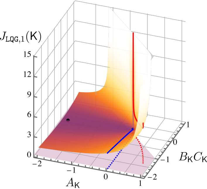
(a)

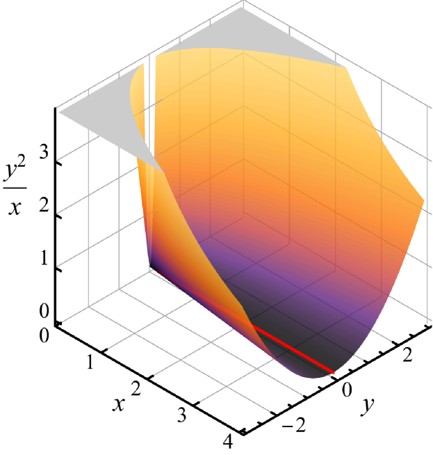
(b)

Figure 2: (a) Discontinuous behavior of LQG cost in 27. The blue and red (dotted) curves correspond to the behaviors for polices in 28a and 28b, respectively, as $\epsilon\downarrow 0$. The blue curve approaches a constant while the red one goes to infinity. The black dot represents the globally optimal policy $A_{\mathsf{K}}^{\star}=1-2\sqrt{2},B_{\mathsf{K}}^{\star}C_{\mathsf{K}}^{\star}=-(1-\sqrt{2})^{2}$ (see Example 4.2). (b) Shape of $f(x,y)$ in 29, where the red line marks the globally optimal points $\{(x,y):x>0,y=0\},$ which can be arbitrarily close to the boundary point $(0,0)$.

Remark 4.1 (Hidden convexity of LQG).

The discontinuous behavior of the LQG cost around its boundary is somewhat surprising to us at first glance, but in retrospect, it also becomes expected. In principle, the LQG cost $J_{\mathtt{LQG},n}({\mathsf{K}})$ behaves similarly to rational functions like

$$f(x,y)=\frac{y^{2}}{x},\qquad\text{dom}(f)=\{(x,y)\in\mathbb{R}^{2}\mid x>0\}.$$ (29)

This function is “discontinuous” at the boundary point $(0,0)$ and will grow unbounded as it approaches other boundary points $(0,y)$ with $y\neq 0$ (see Figure 2(b)). We note that the Hessian of this function is

$$\nabla^{2}f(x,y)=\frac{2}{x^{3}}\begin{bmatrix}y^{2}&\displaystyle-xy\\ \displaystyle-xy&\displaystyle x^{2}\end{bmatrix}\succeq 0,\qquad\forall x>0,y\in\mathbb{R}.$$

This function is convex over its whole domain, thus all stationary points (i.e., $y=0,x>0$) are globally optimal. Note that the convexity of $f(x,y)$ can also be seen from the fact that its epigraph

$$\{(x,y,\gamma)\in\mathbb{R}^{3}\mid\gamma\geq f(x,y),x>0\}=\left\{(x,y,\gamma)\in\mathbb{R}^{3}\mid\begin{bmatrix}\gamma&y\\ y&x\end{bmatrix}\succeq 0,x>0\right\},$$

is convex. Indeed, we will show that a certain form of the epigraph of the LQG control 11 admits a convex representation, and thus LQG optimization is “almost a convex problem” in disguise. The global optimality characterizations in Theorems 4.2 and 4.3 confirm this nice property. Our ECL framework in Part II of this paper will more precisely reveal the hidden convexity of many policy optimization problems in control. Figure 2 illustrates the similar landscape for 27 and 29. ∎

4.2 Main technical results

Before presenting our main technical results, we first recall the closed-form expression to compute the gradient of $J_{\mathtt{LQG},q}({\mathsf{K}})$. If desired, one can further compute its Hessian (and any arbitrary high-order derivatives) since $J_{\mathtt{LQG},q}({\mathsf{K}})$ is real analytical; see [13, Lemma 4.3 & Appendix B.4].

Lemma 4.2 ([13, Lemma 4.2]).

Fix $q\geq 1$ such that ${\mathcal{C}}_{q,0}\neq\varnothing$. For every ${\mathsf{K}}=\begin{bmatrix}0&C_{{\mathsf{K}}}\\ B_{{\mathsf{K}}}&A_{{\mathsf{K}}}\end{bmatrix}\in{\mathcal{C}}_{q,0}$, the gradient of $J_{\mathtt{LQG},q}({\mathsf{K}})$ is given by

$$\frac{\partial J_{\mathtt{LQG},q}({\mathsf{K}})}{\partial A_{{\mathsf{K}}}} =\frac{1}{J_{\mathtt{LQG},q}({\mathsf{K}})}\left(Y_{12}^{{\mathsf{T}}}X_{12}+Y_{22}X_{22}\right),$$ (30a)

$$\frac{\partial J_{\mathtt{LQG},q}({\mathsf{K}})}{\partial B_{{\mathsf{K}}}} =\frac{1}{J_{\mathtt{LQG},q}({\mathsf{K}})}\left(Y_{22}B_{{\mathsf{K}}}V+Y_{22}X_{12}^{{\mathsf{T}}}C^{{\mathsf{T}}}+Y_{12}^{{\mathsf{T}}}X_{11}C^{{\mathsf{T}}}\right),$$ (30b)

$$\frac{\partial J_{\mathtt{LQG},q}({\mathsf{K}})}{\partial C_{{\mathsf{K}}}} =\frac{1}{J_{\mathtt{LQG},q}({\mathsf{K}})}\left(RC_{{\mathsf{K}}}X_{22}+B^{{\mathsf{T}}}Y_{11}X_{12}+B^{{\mathsf{T}}}Y_{12}X_{22}\right),$$ (30c)

where $X_{{\mathsf{K}}}$ and $Y_{{\mathsf{K}}}$, partitioned as

$$X_{{\mathsf{K}}}=\begin{bmatrix}X_{11}&X_{12}\\ X_{12}^{{\mathsf{T}}}&X_{22}\end{bmatrix},\qquad Y_{{\mathsf{K}}}=\begin{bmatrix}Y_{11}&Y_{12}\\ Y_{12}^{{\mathsf{T}}}&Y_{22}\end{bmatrix}$$ (31)

are the unique positive semidefinite solutions to 13a and 13b, respectively.

It has been recently revealed in [13, Theorem 4.2] that the set of stationary points $\{{\mathsf{K}}\in{\mathcal{C}}_{n,0}\mid\nabla J_{\mathtt{LQG},q}({\mathsf{K}})=0\}$ contains strictly suboptimal saddle points for LQG control 11. A positive result is that if a stationary point corresponds to a minimal policy, then it is globally optimal for LQG [13, Theorem 4.3]. However, the analysis in [13, Theorem 4.3] strongly depends on the assumption of minimality, which fails to deal with non-minimal globally optimal policies for LQG. Additionally, it may be difficult to enforce minimality during the policy optimization procedure as argued in [17].

We present our next main technical result of this section, which utilizes the notion of non-degenerate policies for LQG defined in 23 without relying on the minimality assumption.

Theorem 4.2.

Let ${\mathsf{K}}^{\ast}\in{\mathcal{C}}_{n,0}$ be a stationary point of $J_{\mathtt{LQG},n}$ (i.e., $\nabla J_{\mathtt{LQG},n}({\mathsf{K}}^{\ast})=0$). If ${\mathsf{K}}^{\ast}$ is a non-degenerate policy for LQG, then it is a global minimum of $J_{\mathtt{LQG},n}$ over ${\mathcal{C}}_{n,0}$.

Our proof is based on a new ECL framework for epigraphs of nonconvex functions, which will be the focus of Part II of this paper. Essentially, we show that the LQG optimization “almost” behaves as a convex problem. This proof strategy is much more general than [13, Theorem 4.3] that relies on the minimality assumption and Riccati equations. We will use the same proof strategy to establish similar guarantees for nonsmooth and nonconvex $\mathcal{H}_{\infty}$ control in Section 5.2. Theorem 4.2 directly implies that there exist no spurious (local minimum/maximum/saddle points) stationary points of $J_{\mathtt{LQG},n}({\mathsf{K}})$ in ${\mathcal{C}}_{\mathrm{nd},0}$. Indeed, we show that if a policy ${\mathsf{K}}\in{\mathcal{C}}_{\mathrm{nd},0}$ is not globally optimal, then there exists a direction ${\mathsf{V}}$ such that the directional derivative is negative, i.e.,

$$\lim_{t\downarrow 0}\frac{J_{\mathtt{LQG},n}({\mathsf{K}}+t{\mathsf{V}})-J_{\mathtt{LQG},n}({\mathsf{K}})}{t}<0,$$

thus it is always possible to improve over this point via suitable local search algorithms.

Our next result shows that all minimal stationary points must be non-degenerate. In other words, the global optimality in [13, Theorem 4.3] is a special case of Theorem 4.2.

Theorem 4.3.

Let ${\mathsf{K}}^{\ast}\in{\mathcal{C}}_{n,0}$ be a stationary point of $J_{\mathtt{LQG},n}$ (i.e., $\nabla J_{\mathtt{LQG},n}({\mathsf{K}}^{\ast})=0$). If ${\mathsf{K}}^{\ast}$ corresponds to a minimal policy, then it is a non-degenerate policy for LQG, and thus is a global minimum of $J_{\mathtt{LQG},n}$ over ${\mathcal{C}}_{n,0}$.

Proof.

Since ${\mathsf{K}}^{\ast}$ is a minimal policy, the solutions $X_{{\mathsf{K}}^{\ast}}$ and $Y_{{\mathsf{K}}^{\ast}}$ to 13a and 13b are strictly positive definite (cf. [13, Lemma 4.5]). We partition the solutions as 31, and we have $X_{22}\succ 0,Y_{22}\succ 0$. Further, since ${\mathsf{K}}^{\ast}$ is a stationary point, from 30a, we have

$$\frac{\partial{J_{\mathtt{LQG},n}({\mathsf{K}}^{\ast})}}{\partial{A_{\mathsf{K}}}}=\frac{1}{J_{\mathtt{LQG},n}({\mathsf{K}}^{\ast})}(Y_{12}^{{\mathsf{T}}}X_{12}+Y_{22}X_{22})=0\quad\Rightarrow\quad Y_{12}^{{\mathsf{T}}}X_{12}=-Y_{22}X_{22},$$

which implies $X_{12},Y_{12}\in\mathrm{GL}_{n}$.

We next construct matrices $\Gamma$ and $P\in\mathbb{S}^{2n}_{++}$ with $P_{12}\in\mathrm{GL}_{n}$ such that 21a and 21b hold with $\gamma=J_{\mathtt{LQG},n}({\mathsf{K}}^{\ast})$. This will complete our proof of ${\mathsf{K}}^{\ast}\in{\mathcal{C}}_{\mathrm{nd},0}$ by the definition 23. Indeed, we choose

$$P={J_{\mathtt{LQG},n}({\mathsf{K}}^{\ast})}X_{{\mathsf{K}}^{\ast}}^{-1},\qquad\Gamma=C_{\mathrm{cl}}({\mathsf{K}}^{\ast})P^{-1}C_{\mathrm{cl}}({\mathsf{K}}^{\ast})^{{\mathsf{T}}}.$$ (32)

It is not difficulty to verify that they satisfy 21a and 21b with $\gamma=J_{\mathtt{LQG},n}({\mathsf{K}}^{\ast})$ (see the constructions in the proof of Lemma 3.1 in Section A.3). It remains to show $P_{12}\in\mathrm{GL}_{n}$. For this, we infer from $X_{{\mathsf{K}}^{\ast}}X_{{\mathsf{K}}^{\ast}}^{-1}=I$ that

$$X_{11}(X_{{\mathsf{K}}^{\ast}}^{-1})_{12}+X_{12}(X_{{\mathsf{K}}^{\ast}}^{-1})_{22}=0,$$

which implies $(X_{{\mathsf{K}}^{\ast}}^{-1})_{12}\in\mathrm{GL}_{n}$ since $X_{11},X_{12},(X_{{\mathsf{K}}^{\ast}}^{-1})_{22}\in\mathrm{GL}_{n}$. Thus $P_{12}\in\mathrm{GL}_{n}$. ∎

Table 1: Cases of stationary points in LQG control 11.

	Minimal	Non-minimal
Non-degenerate	✓(Example 4.2)	✓(Example 4.3)
Degenerate	✗(cannot exist)	✓(Example 4.4)

Any non-degenerate stationary points are globally optimal (Theorem 4.2), but there may exist degenerate globally optimal policies (Example 4.4).

In the following, we present three examples illustrating Theorems 4.2 and 4.3. Table 1 summarizes different cases of stationary points in LQG control. Our first example below is the case where the globally optimal policy for LQG from the Riccati equation in Theorem A.1 is minimal and non-degenerate.

Example 4.2 (A globally optimal policy that is minimal and non-degenerate).

Consider the same LQG instance in Example 4.1. It is easy to see that the unique positive semidefinite solution to Riccati equation A.23a is $P=\sqrt{2}-1,$ and the Kalman gain is $L=\sqrt{2}-1$. Similarly, the Feedback gain is $K=\sqrt{2}-1$. Then, the globally optimal policy for LQG is given by

$$A_{\mathsf{K}}^{\star}=1-2\sqrt{2},\qquad B_{\mathsf{K}}^{\star}=-1+\sqrt{2},\qquad C_{\mathsf{K}}^{\star}=1-\sqrt{2}.$$

This policy is minimal and thus non-degenerate (cf. Theorem 4.3), i.e., ${\mathsf{K}}^{\star}\in{\mathcal{C}}_{\mathrm{nd},0}$. Therefore, despite the discontinuous boundary behavior in Example 4.1, this LQG instance is well-conditioned and can be solved easily via Riccati equations or LMIs. We can further verify that the globally optimal policies for a class of LQG instances with $A=a,\,B=1,\,C=1,\,Q=1,\,R=1,\,W=1,\,V=1,$ are all non-degenerate for any $a\in\mathbb{R}$; see Section C.2 for computational details. ∎

The following example shows that the notion of non-degenerate policies indeed characterizes a larger class of stationary points, beyond minimal policies, that are globally optimal to 11.

Example 4.3 (A globally optimal policy for LQG that is non-minimal and non-degenerate).

We consider the same example in [13, Example 7], which originates from [76]. In this example, the policy in ${\mathcal{C}}_{n,0}$ is not minimal, but we show it is indeed non-degenerate.

Specifically, we consider the LTI system 1 with

$$A=\begin{bmatrix}0&-1\\ 1&0\end{bmatrix},\qquad B=\begin{bmatrix}1\\ 0\end{bmatrix},\qquad C=\begin{bmatrix}1&-1\end{bmatrix},\qquad W=\begin{bmatrix}1&-1\\ -1&16\end{bmatrix},\qquad V=1,$$

and let the LQG cost be defined by $Q=\begin{bmatrix}4&0\\ 0&0\end{bmatrix},\,R=1.$ This LQG problem satisfies Assumption 1. The positive definite solutions to the Riccati equations A.23 are $P=\begin{bmatrix}1&0\\ 0&4\end{bmatrix},\,S=\begin{bmatrix}2&0\\ 0&2\end{bmatrix},$ and the globally optimal policy is given by

$$A_{{\mathsf{K}}}=\begin{bmatrix}-3&0\\ 5&-4\end{bmatrix},\quad B_{{\mathsf{K}}}=L=\begin{bmatrix}1\\ -4\end{bmatrix},\quad C_{{\mathsf{K}}}=-K=\begin{bmatrix}-2&0\end{bmatrix}.$$ (33)

It is straightforward to verify that $(C_{{\mathsf{K}}},A_{{\mathsf{K}}})$ is not observable. Therefore, the optimal policy for LQG obtained from the Riccati equations is not minimal in this example.

This globally optimal policy 33 turns out to be non-degenerate. Indeed, for the closed-loop system 7 with this optimal policy ${\mathsf{K}}$, the solution to the Lyapunov equation 13a reads as

$$X_{\mathsf{K}}=\begin{bmatrix}5.25&-8&4.25&-8\\ -8&20.25&-8&16.25\\ 4.25&-8&4.25&-8\\ -8&16.25&-8&16.25\end{bmatrix}.$$

It is easy to verify that $X_{\mathsf{K}}\succ 0$ (this is expected since the closed-loop system is controllable thanks to the controllability of $(A_{\mathsf{K}},B_{\mathsf{K}})$) and $(X_{\mathsf{K}}^{-1})_{12}\in\mathrm{GL}_{n}$. Then, the construction in 32 satisfies 21a and 21b with $\gamma=J_{\mathtt{LQG},n}({\mathsf{K}})$. Thus, the non-minimal policy 33 is non-degenerate. ∎

Example 4.4 (A globally optimal policy for LQG that is degenerate).

Similar to minimal policies, our notion of non-degenerate policies depends on state-space realizations. In Example 4.3, some globally optimal policies in ${\mathcal{C}}_{n,0}$ are not connected by similarity transformations. The following two non-minimal policies are both globally optimal:

$${\mathsf{K}}_{1}=\left[\begin{array}[]{c:cc}0&-2&0\\[2.0pt] \hdashline 1&-3&0\\[-2.0pt] -4&5&-4\end{array}\right],\qquad{\mathsf{K}}_{2}=\left[\begin{array}[]{c:cc}0&-2&0\\[2.0pt] \hdashline 1&-3&0\\[-2.0pt] 0&0&-1\end{array}\right],$$

(since they correspond to the same transfer function), but there exists no similarity transformation between ${\mathsf{K}}_{1}$ and ${\mathsf{K}}_{2}$. We have numerically verified in Example 4.3 that ${\mathsf{K}}_{1}$ is non-degenerate; on the other hand, we can further prove that ${\mathsf{K}}_{2}$ is degenerate; see Theorem 4.4 below. This observation raises an interesting question: if a globally optimal policy for LQG is minimal, it must be non-degenerate (cf. Theorem 4.3); for a globally optimal policy for LQG that is not minimal, itself might be degenerate (see ${\mathsf{K}}_{2}$), but does it admit another state-space realization that is non-degenerate (such as ${\mathsf{K}}_{1}$)? Another related question is whether all policies obtained from Riccati equations (i.e., those from Theorem A.1) are non-degenerate. Detailed investigations are left for future work. ∎

4.3 A class of degenerate policies

In Example 4.4, we have identified one degenerate policy that is globally optimal. Due to the existence of saddle points [13, Theorem 4.2], it is expected that there exist sub-optimal degenerate stationary points ${\mathsf{K}}\in{\mathcal{C}}_{n,0}\backslash{\mathcal{C}}_{\mathrm{nd},0}$ for LQG control 11.

We here identify a class of degenerate policies. In particular, the following Theorem 4.4 shows that any stationary point of $J_{\mathtt{LQG},q}$ can be augmented to a stationary point of $J_{\mathtt{LQG},q+q^{\prime}}$ for any $q^{\prime}\geq 1$. Furthermore, any reduced-order minimal policy in ${\mathcal{C}}_{q,0}$ can be augmented to a full-order policy in ${\mathcal{C}}_{n,0}$ that is a degenerate policy.

Theorem 4.4.

Let $0\leq q<n$, and consider a reduced-order policy ${\mathsf{K}}=\begin{bmatrix}0&C_{{\mathsf{K}}}\\ B_{{\mathsf{K}}}&A_{{\mathsf{K}}}\end{bmatrix}\in{\mathcal{C}}_{q,0}$. The following statement holds.

1. For any $q^{\prime}\geq 1$ and any stable $\Lambda\in\mathbb{R}^{q^{\prime}\times q^{\prime}}$, the following augmented policy

   $$\tilde{{\mathsf{K}}}=\left[\begin{array}[]{c:cc}0&C_{{\mathsf{K}}}&0\\[2.0pt] \hdashline B_{{\mathsf{K}}}&A_{{\mathsf{K}}}&0\\[-2.0pt] 0&0&\Lambda\end{array}\right]\in{\mathcal{C}}_{q+q^{\prime},0}$$ (34)

   satisfies $J_{\mathtt{LQG},q+q^{\prime}}\big{(}\tilde{{\mathsf{K}}}\big{)}=J_{\mathtt{LQG},q}({{\mathsf{K}}})$.

2. If the policy ${\mathsf{K}}$ is a stationary point of $J_{\mathtt{LQG},q}$, i.e., $\nabla J_{\mathtt{LQG},q}({\mathsf{K}})=0$, then the augmented policy 34 with any $q^{\prime}\geq 1$ and any stable $\Lambda\in\mathbb{R}^{q^{\prime}\times q^{\prime}}$ is a stationary point of $J_{\mathtt{LQG},q+q^{\prime}}$ over ${\mathcal{C}}_{q+q^{\prime},0}$.

3. Let $q^{\prime}=n-q$. If ${\mathsf{K}}\in{\mathcal{C}}_{q,0}$ is minimal, the augmented policy 34 with any stable $\Lambda\in\mathbb{R}^{q^{\prime}\times q^{\prime}}$ is degenerate, i.e., $\tilde{{\mathsf{K}}}\in{\mathcal{C}}_{n,0}\backslash{\mathcal{C}}_{\mathrm{nd},0}$.

The first statement is straightforward since ${\mathsf{K}}$ and $\tilde{{\mathsf{K}}}$ correspond to the same transfer function in the frequency domain. The second statement has recently been established in [13, Theorem 4.1] which relies on direct gradient computation. The third statement requires some computations around Lyapunov equations and inequalities, which guarantees that the off-diagonal block $P_{12}$ satisfying 21a and 21b with $\gamma=J_{\mathtt{LQG},n}(\tilde{{\mathsf{K}}})$ always has low rank. The details are technically involved. We postpone them to Section D.4 (see Theorem D.1).

We finally present a simple corollary that introduces a class of sub-optimal stationary points that correspond to degenerate policies.

Corollary 4.1.

Suppose the plant 1 is open-loop stable. Let $\Lambda\in\mathbb{R}^{n\times n}$ be stable. Then ${\mathsf{K}}=\left[\begin{array}[]{c:c}0&0\\[2.0pt] \hdashline 0&\Lambda\end{array}\right].$ is a stationary point of $J_{\mathtt{LQG},n}({\mathsf{K}})$ over ${\mathcal{C}}_{n,0}$, and it is degenerate, i.e., ${\mathsf{K}}\in{\mathcal{C}}_{\mathrm{nd},0}$.

This corollary is an immediate consequence from Theorem 4.4, since a zero policy is always a stationary point to LQG control with open-loop stable systems [13, Theorem 4.2]. This zero policy is degenerate, and it will be suboptimal if the globally optimal policy is minimal (since the optimal LQG controller is unique in the frequency domain). We conclude this section with a degenerate policy that corresponds to a strict saddle point.

Example 4.5 (A degenerate policy that corresponds to a strict saddle).

Consider the same LQG instance in Example 4.1. It is straightforward to verify that ${\mathsf{K}}=\begin{bmatrix}0&0\\ 0&-1\end{bmatrix}\in{\mathcal{C}}_{1,0}$ is a stationary point. It is also not difficult to verify that this policy is degenerate. Furthermore, by [13, Theorem 4.3] and [14, Theorem 2], this policy is a strict saddle point and its corresponding Hessian has one negative eigenvalue (indeed, the three eigenvalues are $0$ and $\pm 0.25$). We illustrate this strict saddle in Figure 3. ∎

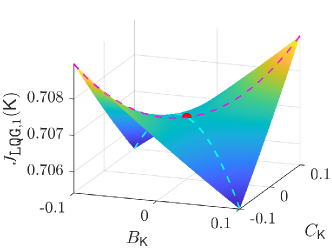
Figure 3: A strict saddle (highlighted as the red point) of LQG optimization landscape in Example 4.5. We fixed $A_{\mathsf{K}}=-1$ and change $B_{\mathsf{K}}\in(-0.1,0.1)$ and $C_{\mathsf{K}}\in(-0.1,0.1)$.

5 Nonsmooth and Nonconvex $\mathcal{H}_{\infty}$ Robust Control

In this section, we turn our focus to the policy optimization for $\mathcal{H}_{\infty}$ control 15. One key difference compared to the LQG control is that the $\mathcal{H}_{\infty}$ cost function $J_{\infty,n}({\mathsf{K}})$ is nonsmooth. We thus need to pay special care to the non-smoothness. However, not surprisingly (or surprisingly) in the spirit of [38], we will show many properties in Section 4 have nonsmooth counterparts for $\mathcal{H}_{\infty}$ control 15, since both $\mathcal{H}_{2}$ and $\mathcal{H}_{\infty}$ norms have similar LMI characterizations (cf. Lemma 3.1 and 3.2). We will also highlight some difficulties in the analysis brought by the unique feature of the bounded real lemma (Lemma 3.2).

We first summarize some basic properties of $\mathcal{H}_{\infty}$ cost function $J_{\infty,n}({\mathsf{K}})$, and demonstrate its non-smoothness using simple examples. Similar to the LQG case, the $\mathcal{H}_{\infty}$ cost function $J_{\infty,n}({\mathsf{K}})$ also exhibits complicated “discontinuous” behavior around its boundary. We then present our main technical result, proving that all Clarke stationary points in the set of non-degenerate policies are globally optimal. The proof also relies on the ECL framework. At the end of this section, we discuss a class of Clarke stationary points that is potentially degenerate and sub-optimal.

5.1 Basic properties and “discontinuous” behavior of the $\mathcal{H}_{\infty}$ cost

The $\mathcal{H}_{\infty}$ cost function $J_{\infty,q}({\mathsf{K}})$ in 14 is known to be nonconvex and also nonsmooth with two possible sources of non-smoothness: One from taking the largest singular value of complex matrices, and the other from maximization over all the frequencies $\omega\in\mathbb{R}$. One could also see the non-smoothness from its max operation in the time domain. Since this is a unique feature in $\mathcal{H}_{\infty}$ control, we highlight it as a fact below.

Fact 5.1.

Fix $q\in\mathbb{N}$ such that ${\mathcal{C}}_{q}\neq\varnothing$. Then, $J_{\infty,q}({\mathsf{K}})$ in 14 is continuous, nonconvex and nonsmooth on ${\mathcal{C}}_{q}$.

We note that the continuity of $J_{\infty,q}({\mathsf{K}})$ in 14 can be viewed from the composition of a convex mapping $\|\cdot\|_{\infty}$ (which is naturally continuous) and the continuous mapping ${\mathsf{K}}\mapsto\mathbf{T}_{zd}$. Indeed, this perspective can ensure strong properties as locally Lipschitz continuity (see Lemma 5.1 below). We here illustrate Fact 5.1 using a simple example.

Example 5.1.

Consider a single-input single-output system with the same dynamics in Example 4.1. In particular, the dynamics in 1 and the performance signal in 2 are given by

$$A=-1,\quad B=1,\quad C=1,\quad Q=1\quad R=1,\quad W=1,\quad V=1.$$

We first consider a static output feedback $u(t)=D_{\mathsf{K}}y(t)$ where $D_{\mathsf{K}}\in\mathbb{R}$. It is easy to see that the set of stabilizing static policies is $\mathcal{C}_{0}=\{D_{\mathsf{K}}\in\mathbb{R}\mid D_{\mathsf{K}}<1\}$. The corresponding $\mathcal{H}_{\infty}$ cost $J_{\infty,0}({\mathsf{K}})$ is shown in Figure 4(a), which shows a nonsmooth point at $D_{\mathsf{K}}=1-\sqrt{3}$ (highlighted by a red point). This policy turns out to be globally optimal for all dynamic policies (see Example 5.3).

We then consider a full-order dynamic output feedback policy. Using the Routh–Hurwitz stability criterion, it is straightforward to derive that

$${\mathcal{C}}_{1} =\left\{\left.{\mathsf{K}}=\begin{bmatrix}D_{{\mathsf{K}}}&C_{{\mathsf{K}}}\\ B_{{\mathsf{K}}}&A_{{\mathsf{K}}}\end{bmatrix}\in\mathbb{R}^{2\times 2}\right|A_{{\mathsf{K}}}+D_{{\mathsf{K}}}<1,\;\;B_{{\mathsf{K}}}C_{{\mathsf{K}}}<-A_{{\mathsf{K}}}+A_{{\mathsf{K}}}D_{{\mathsf{K}}}\right\}.$$ (35)

The corresponding $\mathcal{H}_{\infty}$ cost around the dynamic policy ${\mathsf{K}}_{1}=\begin{bmatrix}1-\sqrt{3}&0\\ 0&-1\end{bmatrix}$ is shown in Figure 4(b), which shows a set of nonsmooth points (highlighted by red lines). ∎

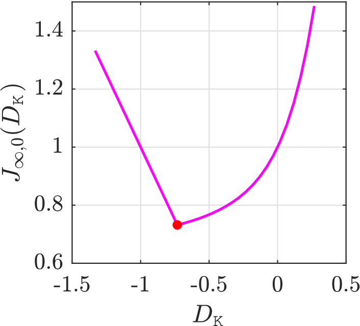
(a) Static output feedback

(b) Dynamic output feedback

Figure 4: Non-smoothness of the $\mathcal{H}_{\infty}$ function in Example 5.1. (a) Static output feedback $u(t)=D_{\mathsf{K}}y(t)$; (b) dynamic output feedback, where we fix $D_{\mathsf{K}}=1-\sqrt{3},A_{{\mathsf{K}}}=-1$ and change $B_{{\mathsf{K}}}\in(-0.6,0.6)$, $C_{{\mathsf{K}}}\in(-0.6,0.6)$.

Despite the non-smoothness, it is known that the $\mathcal{H}_{\infty}$ cost function $J_{\infty,q}({\mathsf{K}})$ is locally Lipschitz and thus differentiable almost everywhere (Figure 4 also suggests this). We can further show $J_{\infty,q}({\mathsf{K}})$ is subdifferentially regular in the sense of Clarke (for self-completeness, we review some fundamentals in nonsmooth optimization in Appendix B). We summarize this property below.

Lemma 5.1 ([48, Proposition 3.1]).

Fix $q\in\mathbb{N}$ such that ${\mathcal{C}}_{q}\neq\varnothing$. The function $J_{\infty,q}({\mathsf{K}})$ in 14 is locally Lipschitz and also subdifferentially regular over $\mathcal{C}_{q}$.

The proof idea in [48, Proposition 3.1] is to view $J_{\infty,q}({\mathsf{K}})$ as a composition of a convex mapping $\|\cdot\|_{\infty}$ and the mapping ${\mathsf{K}}\mapsto\mathbf{T}_{zd}$ that is continuously differentiable over ${\mathsf{K}}$. Then, the subdifferential regularity of $J({\mathsf{K}})$ follows from [39]. We provide some missing details in Section D.5. Similar to the smooth LQG case, $J_{\infty,q}({\mathsf{K}})$ is not coercive due to similarity transformations: it is easy to see that there exists a sequence of policies $\{{\mathsf{K}}_{l}\}\subset\mathcal{C}_{q}$ such that $\lim_{l\to\infty}J_{\infty,q}({\mathsf{K}}_{l})<\infty$ as $\lim_{l\to\infty}\|{{\mathsf{K}}_{l}}\|_{F}=\infty$. We also summarize this as a fact.

Fact 5.2.

Fix $q\in\mathbb{N}$ such that ${\mathcal{C}}_{q}\neq\varnothing$. The function $J_{\infty,q}({\mathsf{K}})$ in 14 is not coercive.

The following example further shows that even when the policies ${\mathsf{K}}$ go to the boundary of $\mathcal{C}_{q}$, the corresponding $\mathcal{H}_{\infty}$ cost might converge to a finite value . This example also shows that the $\mathcal{H}_{\infty}$ cost has “discontinuous” behavior around some boundary points.

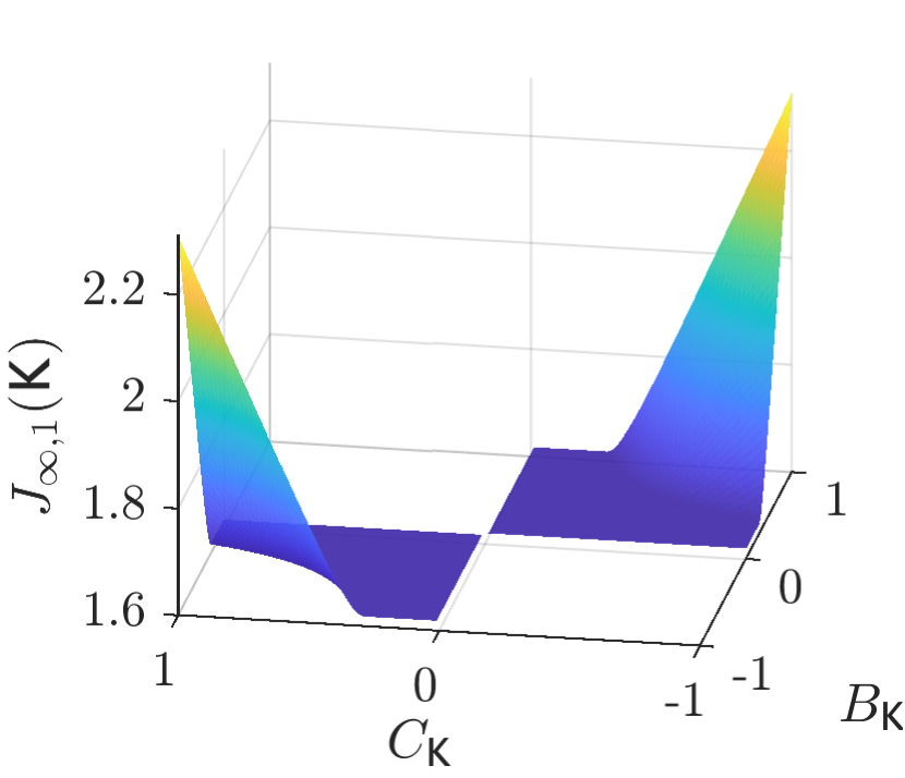
(a)

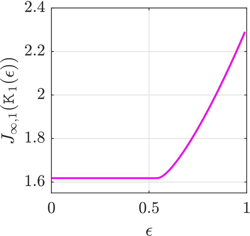
(b)

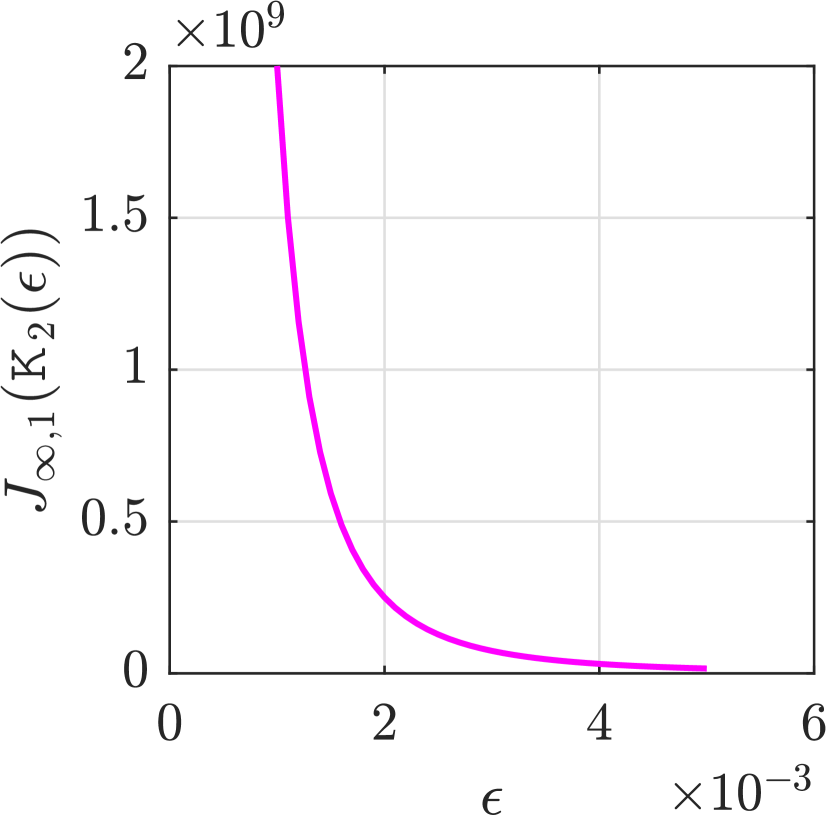
(c)

Figure 5: Boundary behavior of the $\mathcal{H}_{\infty}$ cost in Example 5.2. (a) Shape of $J_{\infty,1}({\mathsf{K}})$, which is fairly flat around $(B_{\mathsf{K}},C_{\mathsf{K}})=(0,0)$, where we fix $A_{\mathsf{K}}=D_{\mathsf{K}}=0$ and change $B_{\mathsf{K}},C_{\mathsf{K}}\in(-1,1)$; (b) Shape of $J_{\infty,1}({\mathsf{K}}_{1}(\epsilon))$ in 36a, which converges to a finite value as $\epsilon\downarrow 0$; (c) Shape of $J_{\infty,1}({\mathsf{K}}_{2}(\epsilon))$ in 36b, which diverges to infinity as $\epsilon\downarrow 0$.

Example 5.2 (Non-coercivity and “discontinuity” of the $\mathcal{H}_{\infty}$ cost).

Consider the same $\mathcal{H}_{\infty}$ instance in Example 5.1. Let ${\mathsf{K}}_{0}=(0,0,0,0)\in\partial\mathcal{C}_{1}$. From 35, the following parameterized policies

$${\mathsf{K}}_{1}(\epsilon)=\begin{bmatrix}0&\epsilon\\ -\epsilon&0\end{bmatrix},\;\;\forall\epsilon\neq 0,$$ (36a)

are all stabilizing, which converges to the boundary point $${\mathsf{K}}_{0} \epsilon\downarrow 0 \lim_{\epsilon\downarrow 0}{\mathsf{K}}_{1}(\epsilon)={\mathsf{K}}_{0} J_{\infty,1}({\mathsf{K}}_{1}(\epsilon)) \epsilon\downarrow 0 J_{\infty,1}(\cdot)$$ as , i.e., . We will show that converges to a finite value as and hence is not coercive; see Figure 5. Indeed, the closed-loop matrices are

$$A_{\mathrm{cl}}({\mathsf{K}}_{1}(\epsilon))= \begin{bmatrix}-1&\epsilon\\ -\epsilon&0\end{bmatrix},\;\;B_{\mathrm{cl}}({\mathsf{K}}_{1}(\epsilon))=\begin{bmatrix}1&0\\ 0&-\epsilon\end{bmatrix},\;\;C_{\mathrm{cl}}({\mathsf{K}}_{1}(\epsilon))=\begin{bmatrix}1&0\\ 0&\epsilon\end{bmatrix},\;\;D_{\mathrm{cl}}({\mathsf{K}}_{1}(\epsilon))=0,$$

and the closed-loop transfer function is

$$\mathbf{T}_{zd}({\mathsf{K}}_{1}(\epsilon))=\frac{1}{s^{2}+s+\epsilon^{2}}\begin{bmatrix}s&-\epsilon^{2}\\ -\epsilon^{2}&-\epsilon^{2}(s+1)\end{bmatrix}\quad\Rightarrow\quad\lim_{\epsilon\downarrow 0}\mathbf{T}_{zd}({\mathsf{K}}_{1}(\epsilon))=\frac{1}{s+1}\begin{bmatrix}1&0\\ 0&0\end{bmatrix}.$$

However, the convergence of these transfer functions is not uniform. After some tedious computation (see Section C.3), we verify that

$$\lim_{\epsilon\downarrow 0}J_{\infty,1}({\mathsf{K}}_{1}(\epsilon)) =\lim_{\epsilon\downarrow 0}\sup_{\omega\in\mathbb{R}}\sigma_{\mathrm{max}}\left(\mathbf{T}_{zd}(j\omega,{\mathsf{K}}_{1}(\epsilon))\right)=\frac{1+\sqrt{5}}{2}.$$

Consider another parameterized stabilizing policies

$${\mathsf{K}}_{2}(\epsilon)=\begin{bmatrix}0&\epsilon+\epsilon^{4}\\ -\epsilon&\epsilon^{2}\end{bmatrix}\in\mathcal{C}_{1},\qquad\forall 1>\epsilon>0.$$ (36b)

which converges to the same boundary point ${\mathsf{K}}_{0}$ as $\epsilon\downarrow 0$. The closed-loop transfer function is

$$\mathbf{T}_{zd}({\mathsf{K}}_{2}(\epsilon))=\frac{1}{s^{2}+(1-\epsilon^{2})s+\epsilon^{5}}\begin{bmatrix}s-\epsilon^{2}&-\epsilon^{2}-\epsilon^{5}\\ -\epsilon^{2}-\epsilon^{5}&-(\epsilon^{2}+\epsilon^{5})(s+1)\end{bmatrix}\;\Rightarrow\;\lim_{\epsilon\downarrow 0}\mathbf{T}_{zd}({\mathsf{K}}_{2}(\epsilon))=\frac{1}{s+1}\begin{bmatrix}1&0\\ 0&0\end{bmatrix}.$$

Again, the convergence of these transfer functions is not uniform. We find that it is tedious to get an analytical expression for their $\mathcal{H}_{\infty}$ norms, but numerical simulation suggests that

$$J_{\infty,1}({\mathsf{K}}_{2}(\epsilon))=\sup_{\omega\in\mathbb{R}}\,\sigma_{\mathrm{max}}(\mathbf{T}_{zd}(j\omega,{\mathsf{K}}_{2}(\epsilon)))\approx\frac{2}{\epsilon^{3}}\qquad\text{if}\;\;0<\epsilon\leq 10^{-1}.$$

This analytical expression agrees with numerical values very well (see Section C.3). For ${\mathsf{K}}_{2}(\epsilon)$, we have $\lim_{\epsilon\downarrow 0}J_{\infty,1}({\mathsf{K}}_{2}(\epsilon))\to\infty$. Therefore, $J_{\infty,1}(\cdot)$ cannot be defined or extended to be continuous at the boundary point ${\mathsf{K}}_{0}$. We illustrate these behaviors in Figure 5. ∎

Similar to Theorem 4.1, the $\mathcal{H}_{\infty}$ cost will diverge to infinity if the sequence of policies converges to a boundary point corresponding to a strictly proper minimal policy. The sequence of policies in 36b was indeed motivated by this result.

Theorem 5.1.

Consider a sequence of policies $\{{\mathsf{K}}_{t}\}_{t=1}^{\infty}\subset{\mathcal{C}}_{n}$ that approaches a boundary point ${\mathsf{K}}_{\infty}\in\partial{\mathcal{C}}_{n}$. If ${\mathsf{K}}_{\infty}$ is minimal, then $\lim_{t\to\infty}J_{\infty,n}({\mathsf{K}}_{t})=\infty$.

This is a consequence of Lemma D.1 since a minimal policy ${\mathsf{K}}$ with $D_{\mathsf{K}}=0$ also leads to a minimal closed-loop system 7 (see Lemma A.10). Finally, similar to the LQG case, Example 5.2 also implies that the sublevel set of the $\mathcal{H}_{\infty}$ cost function $\{{\mathsf{K}}\in{\mathcal{C}}_{n}\mid J_{\infty,n}({\mathsf{K}})\leq\gamma\}$ is not bounded and might not even be closed despite $J_{\infty,n}$ being continuous over its domain. This fact becomes obvious in retrospect since the domain is open and the function is not coercive.

Remark 5.1 (Non-smoothness and hidden convexity in $\mathcal{H}_{\infty}$ control).

Both the smooth LQG cost 10 and nonsmooth $\mathcal{H}_{\infty}$ cost 14 are not coercive and exhibit discontinuity around some non-minimal boundary points. The nonsmooth $J_{\infty,0}({\mathsf{K}})$ in Figure 4(a) appears to be convex (one can indeed verify its convexity), and $J_{\infty,1}({\mathsf{K}})$ has rich geometric symmetry in Figure 4(b). Indeed, our ECL framework will confirm that a certain form of the epigraph of the $\mathcal{H}_{\infty}$ control 15 admits a convex representation, and it is “almost a convex problem” in disguise (see Theorem 5.2). This level of similarity between LQG control 11 and $\mathcal{H}_{\infty}$ control 15 originates the similarity in the LMI characterizations of $\mathcal{H}_{2}$ and $\mathcal{H}_{\infty}$ norms (cf. Lemmas 3.2 and 3.1). In classical literature [38, 77, 68, 41], it is known that the (suboptimal) solutions to LQG control 11 and $\mathcal{H}_{\infty}$ control 15 share similar structures.

Despite their similarities, we here emphasize some key (also well-known) differences. The LQG cost or $\mathcal{H}_{2}$ norm 10 admits a closed-form algebraic expression (i.e., a rational function from the Lyapunov equation). On the other hand, the $\mathcal{H}_{\infty}$ norm 14 depends on the largest singular value over the entire frequency domain, which has no closed-form algebraic expression; even evaluating the $\mathcal{H}_{\infty}$ norm is not a simple task and requires an iterative algorithm (e.g., solving an LMI or using the bisection in [68, Chapter 4.4]). This is already reflected in our computation for the arguably simplest $\mathcal{H}_{\infty}$ case in Example 5.2, which is much more involved than the LQG counterpart in Example 4.1. Consequently, our results below are similar to but less complete than the LQG case. ∎

5.2 Main technical results

Lemma 5.1 justifies that $J({\mathsf{K}})$ is Clarke subdifferentiable. It is now clear from Lemma B.1 that if a dynamic policy ${\mathsf{K}}\in\mathcal{C}_{n}$ is a local minimum of $J_{\infty,n}({\mathsf{K}})$, then ${\mathsf{K}}$ is a Clarke stationary point. Our main goal of this section is to establish a class of Clarke stationary points that are globally optimal to the $\mathcal{H}_{\infty}$ robust control 15, which is a nonsmooth counterpart to Theorem 4.2.

We can indeed compute the Clarke subdifferential of $J_{\infty,q}({\mathsf{K}})$ at any feasible point ${\mathsf{K}}\in\mathcal{C}_{q}$. Let $j\mathbb{R}$ denote the imaginary axis in $\mathbb{C}$. Fix ${\mathsf{K}}\in\mathcal{C}_{q}$, and define

$$\mathcal{Z}=\{s\in j\mathbb{\mathbb{R}}\cup\{\infty\}\mid\sigma_{\max}(\mathbf{T}_{zd}({\mathsf{K}},s))=J_{\infty,q}({\mathsf{K}})\}.$$

For each $s\in\mathcal{Z}$, let $Q_{s}$ be a complex matrix whose columns form an orthonormal basis of the eigenspace of $\mathbf{T}_{zd}({\mathsf{K}},s)\mathbf{T}_{zd}({\mathsf{K}},s)^{{\mathsf{H}}}$ associated with its maximal eigenvalue $J_{\infty,q}^{2}({\mathsf{K}})$. The following lemma characterizes the subdifferential $\partial J_{\infty,q}({\mathsf{K}})$, whose proof is technically invovled. We present the details in Section B.2.

Lemma 5.2.

A matrix $\Phi\in\mathbb{R}^{(m+q)\times(p+q)}$ is a member of $\partial J_{\infty,q}({\mathsf{K}})$ if and only if there exist finitely many $s_{1},\ldots,s_{K}\in\mathcal{Z}$ and associated positive semidefinite Hermitian matrices $Y_{1},\ldots,Y_{K}$ with $\sum_{\kappa=1}^{K}\operatorname{tr}Y_{\kappa}=1$ such that

$$\Phi=\frac{1}{J_{\infty,q}({\mathsf{K}})}\sum_{\kappa=1}^{K}\operatorname{Re}\bigg{\{}\! \left(\begin{bmatrix}0&V^{1/2}\\ 0&0\end{bmatrix}+\begin{bmatrix}C&0\\ 0&I\end{bmatrix}(s_{\kappa}I-A_{\mathrm{cl}}({\mathsf{K}}))^{-1}B_{\mathrm{cl}}({\mathsf{K}})\right)\mathbf{T}_{zd}({\mathsf{K}},s_{\kappa})^{{\mathsf{H}}}Q_{s_{\kappa}}Y_{\kappa}Q_{s_{\kappa}}^{{\mathsf{H}}}$$

$$\quad\cdot\left(\begin{bmatrix}0&0\\ R^{1/2}&0\end{bmatrix}+C_{\mathrm{cl}}({\mathsf{K}})(s_{\kappa}I-A_{\mathrm{cl}}({\mathsf{K}}))^{-1}\begin{bmatrix}B&0\\ 0&I\end{bmatrix}\right)\!\bigg{\}}^{\!{{\mathsf{T}}}}.$$

Note that the subdifferential computation in Lemma 5.2 is much more involved than gradient computations in Lemma 4.2. Still, similar to the LQG case, it is likely that the $\mathcal{H}_{\infty}$ control 15 has many strictly suboptimal Clarke stationary points.

Remark 5.2 (Suboptimal Clarke stationary points in $\mathcal{H}_{\infty}$ control).

If the globally optimal $\mathcal{H}_{\infty}$ policies to 15 are all controllable and observable in $\mathcal{C}_{n}$, and the problem $\min_{{\mathsf{K}}\in\mathcal{C}_{q}}J_{\infty,q}({\mathsf{K}})$ has a solution for some $0\leq q<n$, then there are infinitely many strictly suboptimal Clarke stationary points of $J_{\infty,n}({\mathsf{K}})$ over $\mathcal{C}_{n}$. This result is based on the following characterization: any Clarke stationary point in the space of $\mathcal{C}_{q}$ can be augmented to a full-order Clarke stationary point in $\mathcal{C}_{n}$. We will discuss this lifting characterization in Section 5.3.

Despite the undesirable result in Remark 5.2, our main technical result in this section confirms that if a Clarke stationary point corresponds to a non-degenerate policy in $\mathcal{C}_{\mathrm{nd}}$, then it is globally optimal to 15. This is the nonsmooth counterpart to Theorem 4.2.

Theorem 5.2 (Global optimality).

Let ${\mathsf{K}}\in\mathcal{C}_{\mathrm{nd}}$ be any non-degenerate policy. If ${\mathsf{K}}$ is a Clarke stationary point, i.e., $0\in\partial J_{\infty,n}({\mathsf{K}})$, then it is a global minimizer of $J_{\infty,n}({\mathsf{K}})$ over $\mathcal{C}_{n}$.

Our key proof strategy is based on the same ECL framework for epigraphs of nonconvex functions. Essentially, we show that the $\mathcal{H}_{\infty}$ optimization “almost” behaves as a convex problem. We note that Theorem 5.2 directly implies that there exist no spurious stationary points (local minimum/maximum/saddle) of $J_{\infty,n}({\mathsf{K}})$ in ${\mathcal{C}}_{\mathrm{nd}}$. Indeed, we will show that if a policy ${\mathsf{K}}\in{\mathcal{C}}_{\mathrm{nd}}$ is not globally optimal, then there exists a direction ${\mathsf{V}}$ such that the directional derivative is negative (since $J_{\infty,n}({\mathsf{K}})$ is subdifferential regular, its directional derivative always exists), i.e.,

$$\lim_{t\downarrow 0}\frac{J_{\infty,n}({\mathsf{K}}+t{\mathsf{V}})-J_{\infty,n}({\mathsf{K}})}{t}<0,$$

thus it is always possible to improve over this point via suitable local search algorithms.

In the LQG case (Theorem 4.3), we have shown that any minimal stationary point is non-degenerate, and thus is globally optimal. Motivated by this, we make the following conjecture.

Conjecture 5.1.

Let ${\mathsf{K}}\in{\mathcal{C}}_{n}$ be a Clarke stationary point (i.e., $0\in\partial J_{\infty,n}({\mathsf{K}})$). If ${\mathsf{K}}$ is a minimal policy, then it is non-degenerate, and thus is a global minimum of $J_{\infty,n}({\mathsf{K}})$ over ${\mathcal{C}}_{n}$.

Unlike the smooth LQG case, a rigorous proof of this conjecture (or identifying a counterexample) seems challenging, and we leave it to future work. One main difficulty lies in the non-smoothness of the $\mathcal{H}_{\infty}$ cost and the fact that the computation of the Clarke subdifferential (see Lemma 5.2) is much more involved than computing the gradients for LQG (see Lemma 4.2). This difficulty also appears in the proof of Conjecture 3.1.

We here present an example, adapted from [68, Example 14.3], where the globally optimal $\mathcal{H}_{\infty}$ policy can be computed analytically. In the example below, the globally optimal $\mathcal{H}_{\infty}$ policy from Theorem A.2 turns out to be degenerate.

Example 5.3 (Globally optimal $\mathcal{H}_{\infty}$ policies that are degenerate).

Consider the same $\mathcal{H}_{\infty}$ control instance in Example 5.1. Via analyzing the limiting behavior in Theorem A.2 (see [68, Example 14.3]), we can show that a globally optimal $\mathcal{H}_{\infty}$ policy in this instance is achieved by static output feedback

$$u(t)=D_{\mathsf{K}}^{\star}y(t),\quad\text{with}\quad D_{\mathsf{K}}^{\star}=1-\sqrt{3},$$

and the globally optimal $\mathcal{H}_{\infty}$ cost is $J^{\star}_{\infty,1}=\sqrt{3}-1$. Even for this simple example, the computations for global optimality are quite involved, and we put some details in Section C.2.

It is easy to see that for any $a<0$, the following policy

$$A_{\mathsf{K}}=a,\quad B_{\mathsf{K}}=0,\quad C_{\mathsf{K}}=0,\quad D_{\mathsf{K}}^{\star}=1-\sqrt{3},$$ (37)

is also globally optimal. Via some tedious computations, we can verify that the matrix $P\succ 0$ satisfying the non-strict LMI 25a with $\gamma=\sqrt{3}-1$ must be in the form of

$$P=\begin{bmatrix}1&0\\ 0&p_{3}\end{bmatrix}\succeq 0,$$

where $p_{3}>0$ is any positive value (computational details are presented in Section C.2). Thus, this class of state-space realizations of the globally optimal policy in 37 is degenerate. In Section C.2, via some straightforward yet very tedious computations, we have further verified that the other state-space realizations

$$A_{\mathsf{K}} =a,\quad B_{\mathsf{K}}=b,\quad C_{\mathsf{K}}=0,\quad D_{\mathsf{K}}=1-\sqrt{3}$$

$$A_{\mathsf{K}} =a,\quad B_{\mathsf{K}}=0,\quad C_{\mathsf{K}}=c,\quad D_{\mathsf{K}}=1-\sqrt{3}$$

with $a<0,b\neq 0,c\neq 0$ are all degenerate. ∎

In classical control, it is known that the globally optimal $\mathcal{H}_{\infty}$ controller might not be unique even in the frequency domain [23, Page 406], and this is different from the LQG control which has a unique globally optimal solution in the frequency domain [23, Theorem 14.7]. Here, we use an example from [78] to illustrate this fact.

Example 5.4 (Non-uniqueness of globally optimal $\mathcal{H}_{\infty}$ policies).

Consider the general dynamics A.20 with problem data

$$A =\begin{bmatrix}-1&0\\ 0&-2\end{bmatrix},\;B_{1}=\begin{bmatrix}1\\ 0\end{bmatrix},\;B_{2}=\begin{bmatrix}0\\ -2+a\end{bmatrix},$$

$$C_{1} =\begin{bmatrix}1&1\end{bmatrix},\;C_{2}=\begin{bmatrix}-2&0\end{bmatrix},\;D_{11}=0,\;D_{12}=1,\;D_{21}=1,$$

where $a\in\mathbb{R}$ is a parameter. We note that this system is only stabilizable and detectable (violating Assumption 1). We consider an $\mathcal{H}_{\infty}$ problem by designing a dynamic controller $\mathbf{u}=\mathbf{K}\mathbf{y}$ such that the $\mathcal{H}_{\infty}$ norm of the closed-loop transfer function from $w(t)$ to $z(t)$ is minimized. Via simple frequency-domain algebra, this problem reads as

$$\gamma^{*}=\inf_{\mathbf{K}(s)\in\mathcal{RH}_{\infty}}\;\;\left\|\frac{1}{s+1}+\frac{(s-1)(s-a)}{(s+1)(s+2)}\mathbf{K}(s)\right\|_{\mathcal{H}_{\infty}},$$ (38)

where $\mathbf{K}(s)$ is a stable dynamic controller. This formulation 38 is a standard model-matching problem (one potential solution is via the Nevanlinna–Pick strategy) [79]. When $a=0$, it is clear that $\gamma^{*}\geq\|\frac{1}{0+1}\|_{\infty}=1$ no matter which controller is used. Further, it is not difficult to check that the following two controllers

$$\mathbf{K}_{1}=0,\qquad\mathbf{K}_{2}=\frac{1}{s+3}-1$$

archive the optimal value $\gamma^{*}=1$. Thus, both of them are globally optimal $\mathcal{H}_{\infty}$ controllers to 38. Indeed, there is a family of $\mathbf{K}(s)$ achieving $\gamma^{\star}=1$; see [78] for more details. ∎

5.3 A class of potentially suboptimal Clarke stationary points

As highlighted in Remark 5.2, it is likely that the $\mathcal{H}_{\infty}$ robust control 15 has many suboptimal Clarke stationary points. We here establish an interesting result that any Clarke stationary point of $J_{\infty,q}({\mathsf{K}})$ can be transferred to Clarke stationary points of $J_{\infty,q+q^{\prime}}$ for any $q^{\prime}>0$ with the same $\mathcal{H}_{\infty}$ value. Therefore, it is likely that these new Clarke stationary points are suboptimal over $\mathcal{C}_{q+q^{\prime}}$.

Theorem 5.3.

Let $q\geq 0$ be arbitrary. Suppose there exists ${\mathsf{K}}=\begin{bmatrix}D_{{\mathsf{K}}}&C_{{\mathsf{K}}}\\ B_{{\mathsf{K}}}&A_{{\mathsf{K}}}\end{bmatrix}\in\mathcal{C}_{q}$ such that $0\in\partial J_{\infty,q}({\mathsf{K}})$. Then for any $q^{\prime}\geq 1$ and any stable $\Lambda\in\mathbb{R}^{q^{\prime}\times q^{\prime}}$, the following policy

$$\tilde{{\mathsf{K}}}=\left[\begin{array}[]{c:cc}D_{\mathsf{K}}&C_{{\mathsf{K}}}&0\\[2.0pt] \hdashline B_{{\mathsf{K}}}&A_{{\mathsf{K}}}&0\\[-2.0pt] 0&0&\Lambda\end{array}\right]\in\mathcal{C}_{q+q^{\prime}}$$ (39)

is a Clarke stationary point of $J_{\infty,q+q^{\prime}}$ over $\mathcal{C}_{q+q^{\prime}}$ satisfying $J_{\infty,q+q^{\prime}}\big{(}\tilde{{\mathsf{K}}}\big{)}=J_{\infty,q}(\tilde{{\mathsf{K}}})$.

It is easy to see that $J_{\infty,q+q^{\prime}}\big{(}\tilde{{\mathsf{K}}}\big{)}=J_{\infty,q}(\tilde{{\mathsf{K}}})$ since they correspond to the same transfer function. For the proof of Clarke stationary points, we can directly use the computations of Clarke subdifferential in Lemma 5.2. The proof details are postponed in Section D.6. We conclude this section by highlighting some degenerate and suboptimal Clarke stationary points in $\mathcal{H}_{\infty}$ control.

Remark 5.3 (Degenerate and suboptimal Clarke stationary points in $\mathcal{H}_{\infty}$ control).

Let $q^{\prime}=n-q$ in Theorem 5.3. The augmented policy 39 with any stable $\Lambda\in\mathbb{R}^{q^{\prime}\times q^{\prime}}$ is likely to be degenerate, i.e., $\tilde{{\mathsf{K}}}\in{\mathcal{C}}_{n}\backslash{\mathcal{C}}_{\mathrm{nd}}$; otherwise, Theorem 5.2 ensures that the augmented policy 39 will be globally optimal over the entire ${\mathcal{C}}_{n}$ even ${\mathsf{K}}$ is just a stationary point of $J_{\infty,q}$ over ${\mathcal{C}}_{q}$ ($0\leq q<n$). In other words, it is likely that the augmented policy 39 is a suboptimal Clarke stationary point. We have indeed proved in Theorem 4.4 that the augmented policy 34 is degenerate for LQG control under a mild condition. However, a proof for the case of $\mathcal{H}_{\infty}$ control seems challenging. This difficulty can again be traced back to the non-smoothness of $\mathcal{H}_{\infty}$ norm: we can use the smooth Lyapunov equation 16 to compute the $\mathcal{H}_{2}$ norm, while the bounded real lemma (Lemma 3.2) for the $\mathcal{H}_{\infty}$ norm is non-trivial to manipulate analytically. We also expect that strict saddle points exist for $\mathcal{H}_{\infty}$ cost $J_{\infty,n}({\mathsf{K}})$ over $\mathcal{C}_{n}$, but an explicit example (similar to Example 4.5) is yet to be found. ∎

6 Numerical Experiments

In this section, we present a few numerical experiments to showcase the effectiveness of various methods to approach the global minimum of LQG control 11 and $\mathcal{H}_{\infty}$ robust control 15.

Among different methods, we particularly illustrate the numerical behavior of an existing first-order policy optimization package – HIFOO [80, 51]. HIFOO employs a two-stage approach involving stabilization (spectral abscissa minimization) followed by $\mathcal{H}_{2}$ or $\mathcal{H}_{\infty}$ performance optimization. Both stages utilize nonsmooth and nonconvex optimization techniques with the following components: an initial quasi-Newton algorithm phase to approach a local minimizer, and a subsequent phase including local bundle and gradient sampling methods to verify local optimality (see [80, Section 3] and [81, Section 2] for algorithm details).

The code for our experiments (as well as all the figures in this paper) is available at

https://github.com/soc-ucsd/nonconvex_landscape_in_control.

6.1 LQG optimal control

We here consider four different methods to solve the smooth nonconvex LQG control 11:

1. Analytical solution via solving two Riccati equations (see Theorem A.1).

2. An LMI approach via a change of variables (see [42] or Part II of this paper). We solve the resulting LMI via an interior-point conic solver – Mosek [82].

3. A naive gradient descent policy optimization approach, implemented in [13] (we ran 500 iterations).

4. A sophisticate implementation of first-order policy optimization – HIFOO [80, 51].

We note that the first two methods are model-based, and the last two approaches can in principle be made mode-free via zeroth-order techniques (although we use the model information to compute gradients in our experiments). With known problem data, the globally LQG policy can be very easily computed via two Riccati equations (Theorem A.1), and we use it to benchmark the performance of the other three methods. For our numerical experiments, we consider three LQG instances: 1) a problem with a scalar state variable in Example 4.1; 2) a problem of two-dimensional state with data

$$A=\begin{bmatrix}0&-1\\ 1&0\end{bmatrix},\ B=\begin{bmatrix}1\\ 0\end{bmatrix},\ C=\begin{bmatrix}1&-1\end{bmatrix},\ W=\begin{bmatrix}1&-1\\ -1&16\end{bmatrix},\ V=1,\ Q=\begin{bmatrix}4&0\\ 0&0\end{bmatrix},\ R=1$$

and 3) another problem of three-dimensional state with data

$$A=\begin{bmatrix}1&1&1\\ 0&1&0\\ 1&0&0\end{bmatrix},\ B=\begin{bmatrix}1&0\\ 0&1\\ 0&0\end{bmatrix},\ C=\begin{bmatrix}0&0&1\\ 1&0&0\\ 0&1&1\end{bmatrix},\ W=I,\ V=I,\ Q=I,\ R=I.$$

Table 2: The best LQG costs of three instances returned by different methods.

	Instance 1	Instance 2	Instance 3
Analytical	$0.6966$	$6.1644$	$10.3566$
LMI (Mosek)	$0.6966$	$6.1644$	$10.3566$
Gradient descent	$0.6970$	$6.1644$	$10.5397$
HIFOO	$0.6967$	$6.1644$	$10.3566$

Table 2 lists the final LQG costs obtained through different methods. We observe that the global minimum of LQG costs (as computed analytically in the first row of Table 2) can be easily attained via solving the corresponding LMI (theoretically, Ricatti-based and LMI-based approaches should return solutions with the same performance; but numerically they may return different solutions; as we will see for the $\mathcal{H}_{\infty}$ case in Section 6.2, the corresponding LMIs appear more difficult to solve numerically). The naive gradient descent implementation in [13] converges for the second LQG instance, but fails to return a high-quality solution for the other two instances within 500 iterations.

Interestingly, the HIFOO package has remarkable empirical performance for these three instances, and it returns a globally optimal solution for each of the LQG instances within 120 iterations. Figure 6 illustrates their convergence performance. We note that while the HIFOO package can only certify local optimality, our theoretical guarantees in Theorems 4.2 and 4.3 allow for the certification of global optimality for the resulting policy.

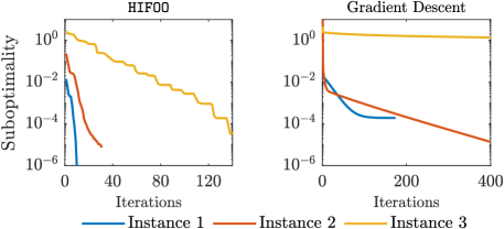
Figure 6: The empirical convergence performance for solving LQG instances. Left: HIFOO [80, 51], where the suboptimality is measured by the LQG cost value gap; Right: Naive gradient descent implementation from [13], where the suboptimality is measured by the gradient norms.

6.2 $\mathcal{H}_{\infty}$ robust control

We next consider the nonsmooth and nonconvex $\mathcal{H}_{\infty}$ robust control 15 using four different methods:

1. Analytical solution via analyzing the limiting solutions from Riccati equations (see Theorem A.2).

2. An LMI approach via a change of variables (see [42] or Part II of this paper). We solve the resulting LMI via two routines i) a general-purpose interior-point conic solver – Mosek [82]; ii) a specialized solver for LMIs – mincx [83].

3. The MATLAB function hinfsyn: there are two options in this function using either i) Riccati iterations [38] or ii) LMIs [26]. Our numerical experiments used their default settings in MATLAB.

4. A sophisticate implementation of first-order policy optimization – HIFOO [80, 51].

As discussed in the main text, obtaining the global minimum of 15 via the first method is often impossible. The limiting analysis is very involved even for very simple instances such as Example 5.3 (see our computational details in Section C.2.). Our numerical experience suggests that the LMIs from $\mathcal{H}_{\infty}$ optimization are often harder to solve than those from $\mathcal{H}_{2}$ optimization; thus we use two different solvers (Mosek and mincx) in the second method. We also report the performance using the built-in function hinfsyn in MATLAB with its default setting. We will see that this implementation may not give the true globally optimal $\mathcal{H}_{\infty}$ performance due to the nature of Riccati iterations (although its performance can be improved by properly tuning its setting in MATLAB). Finally, all these methods above are model-based, while the last method via HIFOO might be adapted to the model-free setting (the details are non-trivial and left for future work).

We test the aforementioned methods to six $\mathcal{H}_{\infty}$ control instances. Three of them are academic examples: 1) the first instance is the same as Example 5.3, for which we have derived its global optimal policy analytically; 2) the second instance has problem data

$$A=\begin{bmatrix}1&1\\ 0&1\end{bmatrix},\ B=\begin{bmatrix}0\\ 1\end{bmatrix},\ C=\begin{bmatrix}1&1\\ 1&0\end{bmatrix},\ W=I,\ V=I,\ Q=I,\ R=I,$$

and the third instance is

$$A=\begin{bmatrix}1&1&1\\ 0&1&0\\ 1&0&0\end{bmatrix},\ B=\begin{bmatrix}1&0\\ 0&1\\ 0&0\end{bmatrix},\ C=\begin{bmatrix}0&0&1\\ 1&0&0\\ 0&1&1\end{bmatrix},\ W=I,\ V=I,\ Q=I,\ R=I.$$

The remaining three instances are benchmark examples from real applications, taken from the COMPl_eib library [84]:

• AC8 [85]: A 9th-order state-space model of the linearized vertical plane dynamics of an aircraft;

• HE1 [86]: A 4th-order model of the longitudinal motion of a VTOL helicopter for typical loading and flight condition at the speed of 135 knots;

• REA2 [87]: A 4th-order chemical reactor model.

Table 3: The $\mathcal{H}_{\infty}$ costs returned by different methods. N/A means the analytical solution is unavailable. The numbers highlighted in bold type denote the best value among all methods up to four significant digits.

Method		$1$-dim	$2$-dim	$3$-dim	AC8	HE1	REA2
Analytical		$\sqrt{3}-1$	N/A	N/A	N/A	N/A	N/A
LMI	mincx	0.7321	$5.4260$	5.0829	1.6165	0.0736	1.1341
	Mosek	0.7321	$5.4267$	$5.0834$	$1.6169$	$0.0738$	1.1341
hinfsyn	LMI	$0.7322$	$5.4288$	$5.0844$	$1.6176$	$0.0739$	1.1341
	Riccati	$0.7381$	$5.4748$	$5.1117$	$1.6258$	$0.0740$	$1.1362$
HIFOO		0.7321	5.4259	$5.0831$	$1.6830$	$0.0827$	1.1341

Table 3 lists the $\mathcal{H}_{\infty}$ costs returned by the methods we tested. As we can observe in the second row of Table 3, the solutions returned by Mosek for the LMIs from $\mathcal{H}_{\infty}$ robust control is often worse than those returned by the specialized solver mincx. We have used the default setting of high-accuracy as the stopping criteria in Mosek, and the solver also reported success for the returned solutions. Similar numerical phenomena for the LMIs from $\mathcal{H}_{2}$ optimization was rare in our experience, indicating that LMIs from $\mathcal{H}_{\infty}$ robust control seem harder to solve numerically using general-purpose conic solvers. This may be related to smooth versus nonsmooth features between $\mathcal{H}_{2}$ and $\mathcal{H}_{\infty}$ optimization, and its detailed analysis is interesting but beyond the scope of this work.

From the third row of Table 3, it is interesting to observe that the solutions from the built-in Matlab routine hinfsyn (especially for the Riccati option) are often not as good as the solutions from LMI (mincx). This is expected since the Riccati option in hinfsyn is based on a bisection strategy, which can only approach the infimum in its limit but the corresponding Riccati equations may not be well-behaved asymptotically. Interestingly again, the HIFOO package has remarkable empirical performance for these $\mathcal{H}_{\infty}$ instances, and it returns high-quality solutions that are often as good as (very close to) those from LMIs. Figure 7 illustrates the convergence behavior of HIFOO for these $\mathcal{H}_{\infty}$ instances.

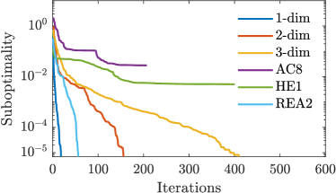
Figure 7: Empirical convergence performance of policy search methods via HIFOO [80, 51] for solving $\mathcal{H}_{\infty}$ instances, where the (local) suboptimality is measured by $\mathcal{H}_{\infty}$ cost gap compared to the best $\mathcal{H}_{\infty}$ value obtained from all methods.

.

From our numerical experiments, we observe another advantage of direct policy optimization like HIFOO: it directly optimizes over a policy class and the resulting policy is often “well-behaved” numerically. For example, for the first $\mathcal{H}_{\infty}$ instance, the solution returned by HIFOO reads

$$J_{\infty,1}({\mathsf{K}}_{\text{{HIFOO}}})=0.73205,\quad{\mathsf{K}}_{\text{{HIFOO}}}=\begin{bmatrix}-0.73205&-0.2123\\ 0&-1.6348\end{bmatrix},$$ (40a)

while the solution returned by hinfsyn (via the default Riccati option) reads

$$J_{\infty,1}({\mathsf{K}}_{\text{riccati}})=0.73814,\quad{\mathsf{K}}_{\text{riccati}}=\begin{bmatrix}0&-0.7111\\ 9.8676&-10.2738\end{bmatrix},$$ (40b)

and the solution returned by hinfsyn (via the default LMI option) reads

$$J_{\infty,1}({\mathsf{K}}_{\text{lmi}})=0.73221,\quad{\mathsf{K}}_{\text{lmi}}=\begin{bmatrix}0&-21.65687\\ 21.6569&-641.8895\end{bmatrix}.$$ (40c)

The solutions in 40b and 40c from hinfsyn correspond to strictly proper dynamic policies, while the solution 40a HIFOO is in fact a static output feedback $u(t)=-0.73205y(t)\approx(1-\sqrt{3})y(t)$ which is almost the same as the analytical solution in Example 5.3. Theoretically, one can use strictly proper dynamic policies to approach the global infimum of $\mathcal{H}_{\infty}$ control (guaranteed by Theorem A.2), but these strictly proper dynamic policies may have large numerical values in their state-space realizations, as shown in 40c and 40b.

7 Conclusions

In this paper, we have examined the nonconvex optimization landscapes of two fundamental control problems: the LQG control with stochastic noises, and $\mathcal{H}_{\infty}$ robust control with adversarial noises. Despite the nonconvexity, our results have characterized the global optimality of non-degenerate stationary points for both LQG and $\mathcal{H}_{\infty}$ optimization over dynamic policies. These results reveal the hidden convexity in LQG control and $\mathcal{H}_{\infty}$ robust control. We have postponed our main proof techniques via a new analysis framework $\mathtt{ECL}$ to Part II of this paper.

There are a few research topics that are worth further investigation. First, we are interested in establishing convergence conditions for local search algorithms to stationary points; this seemingly simple question is nontrivial to address especially due to the non-coercivity of LQG and $\mathcal{H}_{\infty}$ cost functions and their “discontinuity” behavior around the boundary, and thus the existing results [88, 50] cannot be applied immediately. Second, it would be of great interest to design data-driven approaches for checking whether a policy is non-degenerate and avoiding degenerate policies via suitable regularization. Our definition of non-degenerate policies depends on the solution of a matrix inequality. It will be interesting to investigate its further system interpretations and its relationship with classical $\mathcal{H}_{2}$ and $\mathcal{H}_{\infty}$ theories. Finally, the classical literature on controls typically focuses on suboptimal $\mathcal{H}_{\infty}$ policies, and there are good reasons for this (some are practical and some are technical [77, Section 5.1]). From a nonsmooth optimization perspective, it is still extremely interesting to further characterize the global optimality of $\mathcal{H}_{\infty}$ optimization. Following the pioneer work [36, 50], we believe this nonsmooth optimization perspective for $\mathcal{H}_{\infty}$ synthesis will continue to produce fruitful results, especially considering the recent context of model-free data-driven control.

Appendix

This appendix contains many auxiliary results, additional discussions, and technical proofs. We divide it into four parts:

• Appendix A presents some preliminaries in control theory;

• Appendix B presents some preliminaries in nonsmooth optimization;

• Appendix C presents auxiliary results for LQG and $\mathcal{H}_{\infty}$ control;

• Appendix D presents technical proofs that are omitted in the main text.

Appendix A Fundamentals of Control Theory

For self-completeness, we here review some fundamentals on controllability, observability, Lyapunov equations, and LMI characterizations of $\mathcal{H}_{2}$/$\mathcal{H}_{\infty}$ norms. Most of the results below can be found in standard textbooks in control; see [23, Chap 3 & 4 ], [41, 68, 42, 27]. Minor pedagogical contributions might be our explicit emphasis on some subtleties between strict and nonstrict LMIs.

A.1 Controllability and observability

Consider an LTI system parameterized by $(A,B,C,D)\in\mathbb{R}^{n\times n}\times\mathbb{R}^{n\times m}\times\mathbb{R}^{p\times n}\times\mathbb{R}^{p\times m}$,

$$\dot{x} =Ax+Bu,$$ (A.1)

$$y =Cx+Du.$$

The pair $(A,B)$ is called controllable if the following controllability matrix

$$\begin{bmatrix}B&AB&\ldots&A^{n-1}B\end{bmatrix}$$

has full row rank. The pair $(C,A)$ is called observable if the following observability matrix

$$\begin{bmatrix}C\\ CA\\ \vdots\\ CA^{n-1}\end{bmatrix}$$

has full column rank. It is easy to verify that $(A,B)$ is controllable if and only if $(B^{{\mathsf{T}}},A^{{\mathsf{T}}})$ is observable. We also say that the system A.1 is controllable (resp. observable) if the associated pair $(A,B)$ is controllable (resp. $(C,A)$ is observable).

The input-output behavior of A.1 can also be equivalently described in the frequency domain by the transfer matrix $\mathbf{G}(s)=C(sI-A)^{-1}B+D$. It is easy to verify that the transfer matrix $\mathbf{G}(s)$ is invariant under any similarity transformation on the state-space model

$$(A,B,C,D)\mapsto(TAT^{-1},TB,CT^{-1},D),$$

where $T$ is any invertible $n\times n$ real matrix. The system A.1 is called minimal if $(A,B)$ is controllable and $(C,A)$ is observable. This terminology is justified by the following interpretation: if the system A.1 is not minimal, then there exists another state-space model with a smaller state dimension $\hat{n}<n$

$$\dot{\hat{x}} =\hat{A}\hat{x}+\hat{B}u$$

$$y =\hat{C}\hat{x}+Du,$$

such that the input-output behavior is the same as A.1, i.e., $\mathbf{G}(s)=\hat{C}(sI-\hat{A})^{-1}\hat{B}+D.$

In addition to the (Kalman) rank test, there are other equivalent conditions for controllability.

Lemma A.1 ([23, Theorem 3.1]).

Given a matrix pair $(A,B)\in\mathbb{R}^{n\times n}\times\mathbb{R}^{n\times m}$, the following statements are equivalent.

1. $(A,B)$ is controllable.

2. (Pole placement) The eigenvalues of $(A+BK)$ can be arbitrarily assigned by choosing $K\in\mathbb{R}^{m\times n}$.

3. (Invariance under state feedback) $(A+BK,B)$ is controllable for any $K\in\mathbb{R}^{m\times n}$.

In addition to controllability and observability, we will also occasionally encounter the notions of stabilizability and detectability. We say that the pair $(A,B)$ is stabilizable, if there exists a matrix $F$ such that $A+BF$ is stable. We say that $(C,A)$ is detectable, if there exists a matrix $L$ such that $A+LC$ is stable.

A.2 Lyapunov equations

We here review some classical results on Lyapunov equations. Given a real matrix $A\in\mathbb{R}^{n\times n}$ and a symmetric matrix $Q\in\mathbb{S}^{n}$, a standard Lyapunov equation is

$$AX+XA^{{\mathsf{T}}}+Q=0,$$ (A.2)

This is a linear equation in the variable $X$. When the matrix $A$ is stable, we have the following lemma that characterizes the solution to the Lyapunov equation.

Lemma A.2 ([23, Lemma 3.18(i)(ii)]).

Let $A\in\mathbb{R}^{n\times n}$ be stable, i.e., all eigenvalues of $A$ have negative real parts. Then the Lyapunov equation A.2 has a unique solution given by

$$X=\int_{0}^{+\infty}e^{At}Qe^{A^{{\mathsf{T}}}t}\,dt.$$

In addition, $X\succeq 0$ if $Q\succeq 0$, and $X\succ 0$ if $Q\succ 0$.

Another related Lyapunov equation to A.2 is

$$A^{{\mathsf{T}}}Y+YA+Q=0,$$

which replaces $A$ with $A^{{\mathsf{T}}}$. Thus, similar results to Lemma A.2 hold. Furthermore, we can also relate the controllability and observability of a system with the solutions to certain Lyapunov equations.

Lemma A.3 ([23, Lemma 3.18(iii)]).

Let $A\in\mathbb{R}^{n\times n}$ be stable, and let $L_{c}$ and $L_{o}$ be the unique solutions to the following Lyapunov equations

$$AL_{\mathrm{c}}+L_{\mathrm{c}}A^{{\mathsf{T}}}+BB^{{\mathsf{T}}} =0,$$ (A.3)

$$A^{{\mathsf{T}}}L_{\mathrm{o}}+L_{\mathrm{o}}A+C^{{\mathsf{T}}}C =0.$$ (A.4)

Then $(A,B)$ is controllable if and only if $L_{\mathrm{c}}\succ 0$. Similarly, $(C,A)$ is observable if and only if $L_{\mathrm{o}}\succ 0$.

In control theory, the matrices $L_{\mathrm{c}}$ and $L_{\mathrm{o}}$ defined in Lemma A.3 above are called controllability and observability Gramians for the (stable) system A.1, respectively.

Note that in Lemma A.2 and LABEL:{lemma:Lyapunov_controllability_observability}, we have assumed that $A$ is stable. Given the solution to A.2, converse results also exist to establish the stability of $A$. We present one version that is used in our context. These converse results are important when we aim to design a controller that stabilizes a plant (see Remark 3.2).

Lemma A.4 ([23, Lemma 3.19]).

Let $X$ be a solution to the Lyapunov equation A.2.

1. If $Q\succeq 0$ and $X\succ 0$, then $A$ is at least marginally stable, i.e., all eigenvalues of $A$ have non-positive real parts.

2. If $Q\succ 0$ and $X\succ 0$, then $A$ is stable.

3. If $Q=BB^{{\mathsf{T}}}\succeq 0$ with $B\in\mathbb{R}^{n\times m}$, $(A,B)$ is stabilizable and $X\succeq 0$, then $A$ is stable.

The second statement of Lemma A.4 combined with Lemma A.2 implies that the system of linear matrix inequalities $AX+XA^{{\mathsf{T}}}\prec 0,X\succ 0$ is feasible if and only if $A$ is stable (which is the famous canonical Lyapunov inequality). Also, Lemma A.4 immediately leads to a useful alternative characterization.

Lemma A.5.

1. If $(A,B)$ is stabilizable, and the following system of LMIs is feasible,

   $$AX+XA^{{\mathsf{T}}}+BB^{{\mathsf{T}}}\preceq 0,\qquad Y\succeq 0,$$ (A.5)

   then $A$ is stable.

2. If A.5 is feasible with $X\succ 0$, then $A$ is at least marginally stable, i.e., all eigenvalues of $A$ have non-positive real parts.

Proof.

It is clear that $X\succeq 0$ is a solution to the Lyapunov equation $AX+XA^{{\mathsf{T}}}+BB^{{\mathsf{T}}}+B_{0}B_{0}^{{\mathsf{T}}}=0$ for some matrix $B_{0}$. Since $(A,B)$ is stabilizable, we have that $\left(A,\begin{bmatrix}B&B_{0}\end{bmatrix}\right)$ is also stabilizable. The stability of $A$ directly follows from Lemma A.4. ∎

A.3 Characterizations of $\mathcal{H}_{2}$ and $\mathcal{H}_{\infty}$ norms

We here discuss the proofs in Lemma 3.1 and 3.2, and highlight some subtleties between strict and non-strict LMIs.

A.3.1 Characterizations of $\mathcal{H}_{2}$ norms

The results in Lemma 3.1 are classical in control, which can be found in many textbooks. For example, the equivalence in 16 can be found on [42, Page 76], [41, Page 203] and in [23, Lemma 4.6]; more extensive strict LMI characterizations than 17 is summarized in [42, Proposition 3.13] (also see [41, Proposition 6.13]). However, it seems that the nonstrict LMI characterizations in 18 have been less emphasized in the literature.

Here, we reproduce their proofs as they help clarify certain subtleties between strict and nonstrict LMIs for characterizing $\mathcal{H}_{2}$ norms. As previewed in Section 3.1, the proofs below are constructive: the computation of $\|\mathbf{G}\|_{\mathcal{H}_{2}}^{2}$ via 16 is a consequence of the Parseval theorem and Lemma A.2; we then explicitly construct solutions to 16 to prove 17 and 18. Special care needs to be put in when dealing with the converse direction of 18 which requires the controllability of $(A,B)$.

Proof of Statement 1 in Lemma 3.1. The computation of $\|\mathbf{G}\|_{\mathcal{H}_{2}}^{2}$ via 16 is a consequence of the Parseval theorem and Lemma A.2. By definition, we have

$$\|\mathbf{G}\|_{\mathcal{H}_{2}}^{2}=\frac{1}{2\pi}\int_{-\infty}^{\infty}\operatorname{tr}(\mathbf{G}(j\omega)^{{\mathsf{H}}}\mathbf{G}(j\omega))d\omega=\int_{0}^{\infty}\mathrm{trace}(B^{{\mathsf{T}}}e^{A^{{\mathsf{T}}}t}C^{{\mathsf{T}}}Ce^{At}B)dt$$

where the last equality follows the Parseval theorem. Using linearity of the trace, we have

$$\|\mathbf{G}\|_{\mathcal{H}_{2}}^{2}=\operatorname{tr}\!\left(B^{{\mathsf{T}}}\int_{0}^{\infty}e^{A^{{\mathsf{T}}}t}C^{{\mathsf{T}}}Ce^{At}dtB\right)=\mathrm{trace}(B^{{\mathsf{T}}}L_{\mathrm{o}}B),$$

where $L_{\mathrm{o}}$ is the observability Gramian defined in Lemma A.3. From the cyclic property of the trace, we also have

$$\|\mathbf{G}\|_{\mathcal{H}_{2}}^{2}=\operatorname{tr}\!\left(C\int_{0}^{\infty}e^{At}BB^{{\mathsf{T}}}e^{A^{{\mathsf{T}}}t}dtC^{{\mathsf{T}}}\right)=\mathrm{trace}(CL_{\mathrm{c}}C^{{\mathsf{T}}}),$$

where $L_{\mathrm{c}}$ is the controllability Gramian defined in Lemma A.3.

Proof of Statement 2 in Lemma 3.1. This directly follows from a more complete result.

Lemma A.6.

Consider a transfer matrix $\mathbf{G}(s)=C(sI-A)^{-1}B$, where $A\in\mathbb{R}^{n\times n}$ is stable and $C\in\mathbb{R}^{p\times n},B\in\mathbb{R}^{n\times m}$. The following statements are equivalent.

1. $\|\mathbf{G}\|_{\mathcal{H}_{2}}<\gamma$.

2. There exists a symmetric matrix $X$ such that

   $$AX+XA^{{\mathsf{T}}}+BB^{{\mathsf{T}}}\!\prec 0,\quad\operatorname{tr}(CXC^{{\mathsf{T}}})<\gamma^{2}.$$ (A.6)

3. There exist symmetric matrices $P$ and $\Gamma$ such that

   $$\begin{bmatrix}A^{{\mathsf{T}}}P+PA&PB\\ B^{{\mathsf{T}}}P&-\gamma I\end{bmatrix} \prec 0,\;\;\begin{bmatrix}P&C^{{\mathsf{T}}}\\ C&\Gamma\end{bmatrix}\succ 0,\;\;\operatorname{tr}(\Gamma)<\gamma.$$ (A.7)

Proof.

• We first consider the direction 1) $\Rightarrow$ 2). By Statement 1 in Lemma 3.1, we know that $\|\mathbf{G}\|_{\mathcal{H}_{2}}^{2}=\mathrm{tr}(CL_{\mathrm{c}}C^{{\mathsf{T}}})<\gamma^{2}$, where $L_{\mathrm{c}}\succeq 0$ is the controllability Gramian. Since $A$ is stable, there exists $\tilde{X}\succ 0$ such that $A\tilde{X}+\tilde{X}A^{{\mathsf{T}}}\prec 0$. We can then find some $\epsilon>0$ such that

  $$X=L_{\mathrm{c}}+\epsilon\tilde{X}$$ (A.8)

  satisfies $X\succ 0$ and $\mathrm{tr}(CXC^{{\mathsf{T}}})<\gamma^{2}$. Furthermore, we have

  $$AX+XA^{{\mathsf{T}}}+BB^{{\mathsf{T}}}=AL_{\mathrm{c}}+L_{\mathrm{c}}A^{{\mathsf{T}}}+BB^{{\mathsf{T}}}+\epsilon(A\tilde{X}+\tilde{X}A^{{\mathsf{T}}})\prec 0,$$

  which completes the proof of 1) $\Rightarrow$ 2).

  The direction 2 $\Rightarrow$ 1) follows a simple fact: A.6 implies the existence of a nonzero matrix $B_{0}$ such that

  $$AX+XA^{{\mathsf{T}}}+BB^{{\mathsf{T}}}+B_{0}B_{0}^{{\mathsf{T}}}=0,\quad\mathrm{tr}(CXC^{{\mathsf{T}}})<\gamma^{2}.$$

  By Statement 1, we have $\|\mathbf{G}_{e}\|_{\mathcal{H}_{2}}<\gamma$ where $\mathbf{G}_{e}=C(sI-A)^{-1}\begin{bmatrix}B&B_{0}\end{bmatrix}$. Consequently, we have

  $$\|\mathbf{G}\|_{\mathcal{H}_{2}}\leq\|\mathbf{G}_{e}\|_{\mathcal{H}_{2}}<\gamma.$$

• Now we consider the direction 2) $\Rightarrow$ 3). From Lemma A.2, any feasible $X$ in A.6 is strictly positive definite. Then, from a feasible $X\succ 0$, we can find some $\epsilon>0$ such that

  $$\Gamma=\frac{1}{\gamma}CXC^{{\mathsf{T}}}+\epsilon I\qquad\text{and}\qquad P=\gamma X^{-1}$$ (A.9)

  satisfy $\Gamma\succ 0$, $P\succ 0$ and $\operatorname{tr}(\Gamma)<\gamma$. We further infer that $\Gamma\succ\frac{1}{\gamma}CXC^{{\mathsf{T}}}=CP^{-1}C^{{\mathsf{T}}}$ and

  $$A^{{\mathsf{T}}}P+PA+\frac{1}{\gamma}PBB^{{\mathsf{T}}}P=\gamma X^{-1}\left(AX+XA^{{\mathsf{T}}}+BB^{{\mathsf{T}}}\right)X^{-1}\!\prec 0,$$

  By using Schur complements, these two inequalities are equivalent to those in A.7.

  The direction 3) $\Rightarrow$ 2) follows directly if we notice that, given $P$ and $\Gamma$ satisfying A.7, the matrix $X=\gamma P^{-1}$ satisfies A.6. The proof is now complete. ∎

Proof of Statement 3 in Lemma 3.1. For this, we establish the following result.

Lemma A.7.

Consider a transfer matrix $\mathbf{G}(s)=C(sI-A)^{-1}B$, where $A\in\mathbb{R}^{n\times n}$ is stable and $C\in\mathbb{R}^{p\times n},B\in\mathbb{R}^{n\times m}$. The following two statements are equivalent.

1. There exists $X\succ 0$ such that

   $$AX+XA^{{\mathsf{T}}}+BB^{{\mathsf{T}}}\!\preceq 0,\quad\mathrm{tr}(CXC^{{\mathsf{T}}})\leq\gamma^{2}.$$ (A.10)

2. There exist $P\succ 0$ and $\Gamma\succeq 0$ such that

   $$\begin{bmatrix}A^{{\mathsf{T}}}P+PA&PB\\ B^{{\mathsf{T}}}P&-\gamma I\end{bmatrix} \preceq 0,\;\;\begin{bmatrix}P&C^{{\mathsf{T}}}\\ C&\Gamma\end{bmatrix}\succeq 0,\;\;\mathrm{tr}(\Gamma)\leq\gamma.$$ (A.11)

The two matrices $X$ and $P$ can be related by $X=\gamma P^{-1}$. Furthermore, either one (and thus both) of A.10 and A.11 guarantees $\|\mathbf{G}\|_{\mathcal{H}_{2}}\leq\gamma$; the converse is true when $(A,B)$ is controllable.

Proof.

We use similar constructions as those in Lemma A.6.

• 1) $\Rightarrow$ 2): From the solution $X\succ 0$, we use the same construction in A.9 with $\epsilon=0$. Then, we have $\mathrm{tr}(\Gamma)\leq\gamma$. We further infer that $\Gamma=CP^{-1}C^{{\mathsf{T}}}\Rightarrow\Gamma-CP^{-1}C^{{\mathsf{T}}}=0\succeq 0$ and

  $$A^{{\mathsf{T}}}P+PA+\frac{1}{\gamma}PBB^{{\mathsf{T}}}P=\gamma X^{-1}\left(AX+XA^{{\mathsf{T}}}+BB^{{\mathsf{T}}}\right)X^{-1}\!\preceq 0.$$

  The Schur complement confirms that $P$ and $\Gamma$ satisfy the nonstrict LMI A.11.

• The direction 2) $\Rightarrow$ 1) follows the same construction $X=\gamma P^{-1}\succ 0$. Simple calculations confirm that $\mathrm{tr}(CXC^{{\mathsf{T}}})=\gamma\mathrm{tr}(CP^{-1}C^{{\mathsf{T}}})\leq\gamma\mathrm{tr}(\Gamma)\leq\gamma^{2}$ and

  $$AX+XA^{{\mathsf{T}}}+BB^{{\mathsf{T}}}=\frac{1}{\gamma}X\left(A^{{\mathsf{T}}}P+PA+\frac{1}{\gamma}PBB^{{\mathsf{T}}}P\right)X\preceq 0.$$

We next show that A.10 implies $\|\mathbf{G}\|_{\mathcal{H}_{2}}\leq\gamma$. From A.10, we can find a (possibly zero) matrix $B_{0}$ such that

$$AX+XA^{{\mathsf{T}}}+BB^{{\mathsf{T}}}+B_{0}B_{0}^{{\mathsf{T}}}=0,\;\;\operatorname{tr}(CXC^{{\mathsf{T}}})\leq\gamma^{2}.$$

By Statement 1 in Lemma 3.1, we know that $\|\mathbf{G}_{e}\|_{\mathcal{H}_{2}}\leq\gamma$ where $\mathbf{G}_{e}=C(sI-A)^{-1}\begin{bmatrix}B&B_{0}\end{bmatrix}$. Consequently, we have $\|\mathbf{G}\|_{\mathcal{H}_{2}}\leq\|\mathbf{G}_{e}\|_{\mathcal{H}_{2}}\leq\gamma.$

We finally show that if $\|\mathbf{G}\|_{\mathcal{H}_{2}}\leq\gamma$ and $(A,B)$ is controllable, then A.10 holds with $X\succ 0$. By Statement 1 in Lemma 3.1, we know $\|\mathbf{G}\|_{\mathcal{H}_{2}}^{2}=\mathrm{tr}(CL_{\mathrm{c}}C^{{\mathsf{T}}})\leq\gamma^{2}$, where $L_{\mathrm{c}}$ satisfies A.3. Since $(A,B)$ is controllable, we know $L_{\mathrm{c}}\succ 0$ by Lemma A.3. The proof is finished by choosing

$$X=L_{\mathrm{c}}\succ 0$$ (A.12)

which satisfies the nonstrict LMI A.10, i.e., $AX+XA^{{\mathsf{T}}}+BB^{{\mathsf{T}}}\!=0\preceq 0,\ \mathrm{tr}(CXC^{{\mathsf{T}}})\leq\gamma^{2}.$ ∎

Remark A.1 (Strict vs nonstrict LMIs in $\mathcal{H}_{2}$ norm).

From the constructions in Lemma A.6 and A.7, it is clear that $X\succ 0$ and $P\succ 0$ are very important; otherwise their inverses may not exist. In the strict LMI A.6, we know from Lemma A.2 that all feasible solutions $X$ must be positive definite. Although the solution to A.3 may be only positive semidefinite, the perturbed matrix A.8 is guaranteed to be strictly positive definite while also satisfying the strict LMI. On the other hand, if $(A,B)$ is controllable, the solution to A.3 (i.e., the controllability Gramian) is guaranteed to be positive definite. In this case, no perturbation is required in A.12 to construct the solutions to A.10 and A.11, which allows us to obtain non-strict LMIs. $\square$

Throughout Lemma A.6 and A.7, the observability of $(C,A)$ is not required. If $(C,A)$ is observable, we have stronger results that will be presented in Lemma A.9 and A.8.

Lemma A.8.

Consider a transfer matrix $\mathbf{G}(s)=C(sI-A)^{-1}B$ where $A$ is stable. Suppose $(C,A)$ is observable. If A.11 holds with $\gamma=\|\mathbf{G}\|_{\mathcal{H}_{2}}$, $P\succ 0$ and $\Gamma\succeq 0$, then $(A,B)$ is controllable.

Proof.

From Lemma A.7, we see that A.10 holds with $X=\gamma P^{-1}\succ 0$. Then, there exists a matrix $B_{0}$ such that $AX+XA^{{\mathsf{T}}}+BB^{{\mathsf{T}}}+B_{0}B_{0}^{{\mathsf{T}}}=0$. By Statement 1 in Lemma 3.1, we have

$$\gamma^{2}=\left\|\mathbf{G}\|_{\mathcal{H}_{2}}^{2}\leq\|C(sI-A)^{-1}\begin{bmatrix}B,B_{0}\end{bmatrix}\right\|_{\mathcal{H}_{2}}^{2}=\mathrm{tr}(CXC^{{\mathsf{T}}})\leq\gamma^{2}.$$

We must have $\|C(sI-A)^{-1}B_{0}\|_{\mathcal{H}_{2}}^{2}=0$, i.e., $C(sI-A)^{-1}B_{0}=0$ is a zero transfer matrix. Since $(C,A)$ is observable, we get $B_{0}=0$. Therefore, both inequalities in A.10 hold with equalities for $X=\gamma P^{-1}\succ 0$. We see that $X$ is just the controllability Gramian $L_{\mathrm{c}}$, and Lemma A.3 ensures that $(A,B)$ is controllable. ∎

Lemma A.9.

Consider a transfer matrix $\mathbf{G}(s)=C(sI-A)^{-1}B$ where $A$ is stable. If $(A,B,C)$ is controllable and observable, then there exist unique $P\succ 0$ and $\Gamma\succeq 0$ satisfying A.11 with $\gamma=\|\mathbf{G}\|_{\mathcal{H}_{2}}$.

Proof.

Let $P\succ 0$ and $\Gamma\succeq 0$ satisfy A.11, and let $X=\gamma P^{-1}$ so that it satisfies A.10. From the proof of Lemma A.8, any $X\succ 0$ satisfying A.10 will necessarily be equal to the controllability Gramian $L_{\mathrm{c}}$. Consequently, the matrix $P=\gamma L_{\mathrm{c}}^{-1}$ is unique. To show the uniqueness of $\Gamma$, we note that A.11 implies $\Gamma-CP^{-1}C^{{\mathsf{T}}}\succeq 0$, which further leads to

$$\gamma=\gamma^{-1}\operatorname{tr}(CL_{\mathrm{c}}C^{{\mathsf{T}}})=\operatorname{tr}(CPC^{{\mathsf{T}}})\leq\operatorname{tr}(\Gamma)\leq\gamma.$$

As a result, $\operatorname{tr}(\Gamma-CP^{-1}C^{{\mathsf{T}}})=0$, which implies $\Gamma$ is equal to $CP^{-1}C^{{\mathsf{T}}}$ and therefore is unique. ∎

We present an example below showing that if $(C,A)$ is not observable, then the solution set to the nonstrict LMI A.11 is not a singleton with $\gamma=\|\mathbf{G}\|_{\mathcal{H}_{2}}$.

Example A.1.

Consider a second-order system with matrices

$$A=\begin{bmatrix}-1&0\\ 2&-2\end{bmatrix},\qquad B=\begin{bmatrix}1\\ 0\end{bmatrix},\qquad C=\begin{bmatrix}1&0\end{bmatrix}.$$

This system is controllable but not observable (only detectable). The unique solution to 16a is

$$L_{\mathrm{c}}=\frac{1}{6}\begin{bmatrix}3&2\\ 2&2\end{bmatrix},$$

which is positive definite as expected. The corresponding $\mathcal{H}_{2}$ norm is $\gamma=\|\mathbf{G}\|_{\mathcal{H}_{2}}=\frac{\sqrt{2}}{2}$. It is straightforward to verify that $X=L_{c}\succ 0$ satisfies A.10 with $\gamma=\frac{\sqrt{2}}{2}$. To see the extra flexibility, we compute

$$AX+XA^{{\mathsf{T}}}=\begin{bmatrix}-1&0\\ 0&0\end{bmatrix},\quad BB^{{\mathsf{T}}}=\begin{bmatrix}1&0\\ 0&0\end{bmatrix},\quad C^{{\mathsf{T}}}C=\begin{bmatrix}1&0\\ 0&0\end{bmatrix}.$$

The above equalities suggest that the bottom right element has extra freedom for the inequality in A.10. In particular, let us choose

$$X_{t}=X+\frac{1}{6}\begin{bmatrix}0&0\\ 0&t\end{bmatrix}=\frac{1}{6}\begin{bmatrix}3&2\\ 2&2+t\end{bmatrix}\succ 0,\quad\forall t\geq 0.$$

It is straightforward to verify that

$$AX_{t}+X_{t}A^{{\mathsf{T}}}+BB^{{\mathsf{T}}}=-\frac{2}{3}\begin{bmatrix}0&0\\ 0&t\end{bmatrix}\preceq 0,\quad\mathrm{tr}(CX_{t}C^{{\mathsf{T}}})=\frac{1}{2},\quad\forall t\geq 0.$$

Thus, $X_{t}\succ 0,\forall t\geq 0$ is feasible to A.10. For each $X_{t}$, the construction A.9 with $\epsilon=0$ is feasible to the nonstrict LMI A.11 with $\gamma=\frac{\sqrt{2}}{2}$. ∎

A.3.2 Characterizations of $\mathcal{H}_{\infty}$ norm

The bounded real lemma in Lemma 3.2 is a classical result in control, which establishes equivalence between a frequency-domain inequality (i.e., $\mathcal{H}_{\infty}$ norm) and the algebraic feasibility of LMIs in the state-space domain. This result is covered in many modern control textbooks; see, for example, [68, Corollary 12.3] for strict versions and [42, Lemma 2.11] for nonstrict versions.

There are different proofs for Lemma 3.2. The constructive proof in [41, Lemma 7.3] and [68, Corollary 12.3] for strict versions reveals some of the deepest relationships in linear systems theory (such as Riccati operator and Hamiltonian matrix), which is not easily accessible for readers outside control. An alternative elegant proof based on convex duality first appeared in [69], and this duality perspective has been further developed in [42, Lemma 2.11], [70, Section 6] and [71, 89, 90]. We adopt the duality techniques in [69, 70, 71] to highlight the subtleties between strict and non-strict LMIs.

Before presenting the proof of Lemma 3.2, we introduce a few equivalent LMI formulations to 19 and 20. First, via Schur complement, 19 is equivalent to the following LMI

$$\begin{bmatrix}A^{{\mathsf{T}}}P+PA&PB\\ B^{{\mathsf{T}}}P&-\gamma I\end{bmatrix}+\frac{1}{\gamma}\begin{bmatrix}C^{{\mathsf{T}}}\\ D^{{\mathsf{T}}}\end{bmatrix}\begin{bmatrix}C&D\end{bmatrix}\prec 0.$$ (A.13a)

Via a scaling argument $$\gamma P\to P$$, A.13a is equivalent to the following LMI

$$\begin{bmatrix}A^{{\mathsf{T}}}P+PA&PB\\ B^{{\mathsf{T}}}P&-\gamma^{2}I\end{bmatrix}+\begin{bmatrix}C^{{\mathsf{T}}}\\ D^{{\mathsf{T}}}\end{bmatrix}\begin{bmatrix}C&D\end{bmatrix}\prec 0,$$ (A.13b)

which is further equivalent to the following Riccati inequality (again via Schur complement)

$$A^{{\mathsf{T}}}P+PA+C^{{\mathsf{T}}}C-(PB+C^{{\mathsf{T}}}D)(D^{{\mathsf{T}}}D-\gamma^{2}I)^{-1}(PB+C^{{\mathsf{T}}}D)^{{\mathsf{T}}}\prec 0,\;D^{{\mathsf{T}}}D\prec\gamma^{2}I.$$ (A.13c)

Similarly, the nonstrict LMI 20 is equivalent to

$$\begin{bmatrix}A^{{\mathsf{T}}}P+PA&PB\\ B^{{\mathsf{T}}}P&-\gamma^{2}I\end{bmatrix}+\begin{bmatrix}C^{{\mathsf{T}}}\\ D^{{\mathsf{T}}}\end{bmatrix}\begin{bmatrix}C&D\end{bmatrix}\preceq 0.$$ (A.14)

We are now ready to prove Lemma 3.2.

Proof of the sufficient conditions in Lemma 3.2: For both the strict LMI 19 and nonstrict LMI 20, the “if ” direction is relatively straightforward and involves a control-theoretic interpretation for the variable $P$.

Consider the LTI system A.1 with $x(0)=0$. When $A$ is stable, its $\mathcal{H}_{\infty}$ norm $\|C(sI-A)^{-1}B+D\|_{\mathcal{H}_{\infty}}\leq\gamma$ if and only if

$$\|y\|_{2}^{2}\leq\gamma^{2}\|u\|_{2}^{2},\qquad\forall u\in\mathcal{L}_{2}[0,\infty).$$ (A.15)

We next show A.15 is true if there exists a $P\succ 0$ such that A.14 holds. Pre-multiplying A.14 by $\begin{bmatrix}x(t)^{{\mathsf{T}}},u(t)^{{\mathsf{T}}}\end{bmatrix}$ and postmultiplying A.14 by $\begin{bmatrix}x(t)^{{\mathsf{T}}},u(t)^{{\mathsf{T}}}\end{bmatrix}^{{\mathsf{T}}}$ lead to

$$x^{{\mathsf{T}}}P(Ax+Bu)+(Ax+Bu)^{{\mathsf{T}}}Px-\gamma^{2}u^{{\mathsf{T}}}u+y^{{\mathsf{T}}}y\leq 0,\qquad\forall t\geq 0.$$ (A.16)

We introduce the storage function $V:\mathbb{R}^{n}\to\mathbb{R}$ defined by $V(x)=x^{{\mathsf{T}}}Px$. Then, A.16 implies the so-called dissipation inequality

$$\frac{d}{dt}V(x(t))+y^{{\mathsf{T}}}y\leq\gamma^{2}u^{{\mathsf{T}}}u,\qquad\forall t\geq 0.$$ (A.17)

Integrating over an interval $[0,T]$, and recalling that $x(0)=0$, we have

$$V(x(T))+\int_{0}^{T}y^{{\mathsf{T}}}y\,dt\leq\gamma^{2}\int_{0}^{T}u^{{\mathsf{T}}}u\,dt.$$

Note that $P\succ 0$ implies $V(x(T))\geq 0$, which further leads to $\int_{0}^{T}y^{{\mathsf{T}}}y\,dt\leq\gamma^{2}\int_{0}^{T}u^{{\mathsf{T}}}u\,dt$. Letting $T\rightarrow+\infty$ proves A.15.

Suppose there exists a $P\succ 0$ such that A.13b holds. Then we can find some $\epsilon>0$ such that

$$\begin{bmatrix}A^{{\mathsf{T}}}P+PA&PB\\ B^{{\mathsf{T}}}P&-(\gamma-\epsilon)^{2}I\end{bmatrix}+\begin{bmatrix}C^{{\mathsf{T}}}\\ D^{{\mathsf{T}}}\end{bmatrix}\begin{bmatrix}C&D\end{bmatrix}\preceq 0.$$

By the same construction in A.15 and A.16, we get

$$\|y\|_{2}^{2}\leq(\gamma-\epsilon)^{2}\|u\|_{2}^{2},\qquad\forall u\in\mathcal{L}_{2}[0,+\infty),$$

which implies $\|C(sI-A)^{-1}B+D\|_{\mathcal{H}_{\infty}}\leq\gamma-\epsilon<\gamma$.

Proof of the necessary conditions in Lemma 3.2: The “only if” direction in 19 and 20 are more involved to prove. We here adopt the convex duality techniques in [69, 70, 71] to highlight some subtleties between strict and non-strict LMIs.

Let us construct a primal and dual perspective of computing $\mathcal{H}_{\infty}$ norms [70]. Consider the LTI system A.1 with $x(0)=0$. Let $A$ be stable and $\gamma\geq\|C(sI-A)^{-1}B+D\|_{\mathcal{H}_{\infty}}$. For any $u\in\mathcal{L}_{2}[0,+\infty)$, both the state $x(t)$ and output $y(t)$ have finite energy. Therefore, the following quantities are well-defined

$$Z_{11}=\int_{0}^{\infty}x(t)x(t)^{{\mathsf{T}}}dt,\quad Z_{12}=\int_{0}^{\infty}x(t)u(t)^{{\mathsf{T}}}dt,\quad Z_{22}=\int_{0}^{\infty}u(t)u(t)^{{\mathsf{T}}}dt.$$

It is straightforward to verify that

$$AZ_{11}+BZ_{12}^{{\mathsf{T}}}+Z_{11}A^{{\mathsf{T}}}+Z_{12}B^{{\mathsf{T}}}=\int_{0}^{\infty}\frac{d}{dt}(x(t)x(t)^{{\mathsf{T}}})=0$$

and

$$\begin{bmatrix}Z_{11}&Z_{12}\\ Z_{12}^{{\mathsf{T}}}&Z_{22}\end{bmatrix}=\int_{0}^{\infty}\begin{bmatrix}x(t)\\ u(t)\end{bmatrix}\begin{bmatrix}x(t)\\ u(t)\end{bmatrix}^{{\mathsf{T}}}dt\succeq 0,\qquad\operatorname{tr}\left(\begin{bmatrix}C&D\end{bmatrix}\begin{bmatrix}Z_{11}&Z_{12}\\ Z_{12}^{{\mathsf{T}}}&Z_{22}\end{bmatrix}\begin{bmatrix}C^{{\mathsf{T}}}\\ D^{{\mathsf{T}}}\end{bmatrix}\right)=\int_{0}^{\infty}y(t)^{{\mathsf{T}}}y(t)dt.$$

We now define two sets

$$\mathcal{V} =\left\{Z\succeq 0\mid Z=\int_{0}^{\infty}\begin{bmatrix}x(t)\\ u(t)\end{bmatrix}\begin{bmatrix}x(t)\\ u(t)\end{bmatrix}^{{\mathsf{T}}}dt\;\;\text{for some}\;\;u\in\mathcal{L}_{2}[0,\infty)\;\text{to \lx@cref{creftype~refnum}{eq:App_dynamics} with $x(0)=0$}\right\},$$

$$\mathcal{V}_{\mathrm{sdp}} =\left\{Z\succeq 0\mid AZ_{11}+BZ_{12}^{{\mathsf{T}}}+Z_{11}A^{{\mathsf{T}}}+Z_{12}B^{{\mathsf{T}}}=0\right\}.$$

It is clear that $\mathcal{V}\subseteq\mathcal{V}_{\mathrm{sdp}}$. In fact, it is proved in [71, Lemma 3.4] that $\mathcal{V}_{\mathrm{sdp}}=\mathrm{cl}\,\mathcal{V}$.

We then consider the following semidefinite optimization problem

$$p^{\star}=\sup_{Z} \operatorname{tr}\left(\begin{bmatrix}C&D\end{bmatrix}\begin{bmatrix}Z_{11}&Z_{12}\\ Z_{12}^{{\mathsf{T}}}&Z_{22}\end{bmatrix}\begin{bmatrix}C^{{\mathsf{T}}}\\ D^{{\mathsf{T}}}\end{bmatrix}\right)$$ (A.18)

subject to $$AZ_{11}+BZ_{12}^{{\mathsf{T}}}+Z_{11}A^{{\mathsf{T}}}+Z_{12}B^{{\mathsf{T}}}=0,$$

$$\operatorname{tr}(Z_{22})=1,\quad\begin{bmatrix}Z_{11}&Z_{12}\\ Z_{12}^{{\mathsf{T}}}&Z_{22}\end{bmatrix}\succeq 0.$$

The fact $\mathcal{V}_{\mathrm{sdp}}=\mathrm{cl}\,\mathcal{V}$ implies that $p^{\star}$ is equal to the squared $\mathcal{H}_{\infty}$ norm of the transfer matrix $C(sI-A)^{-1}B+D$. It can be verified that the Lagrangian dual of A.18 is

$$d^{\star}=\inf_{\beta,P} \beta$$ (A.19)

subject to $$\begin{bmatrix}A^{{\mathsf{T}}}P+PA&PB\\ B^{{\mathsf{T}}}P&-\beta I\end{bmatrix}+\begin{bmatrix}C^{{\mathsf{T}}}\\ D^{{\mathsf{T}}}\end{bmatrix}\begin{bmatrix}C&D\end{bmatrix}\preceq 0.$$

Since $A$ is stable, we have a positive definite solution $P\succ 0$ to $A^{{\mathsf{T}}}P+PA=-tI,\forall t>0$. Therefore, we can construct a strict feasible solution to the dual SDP A.19 by letting $\beta>0$ and $t>0$ be sufficiently large and letting $P$ be the positive definite solution to $A^{{\mathsf{T}}}P+PA=-tI$. [91, Theorem 2.4.1] then justifies that strong duality holds for A.19 and A.18 , i.e.,

$$p^{\star}=d^{\star}.$$

To show the “only if” direction of the non-strict LMI 20 in Lemma 3.2, we employ the result proved in [71, Proposition 3.3] that the primal SDP A.18 is strictly feasible if and only if $(A,B)$ is controllable. Then, since the strict feasibility of the primal SDP A.18 implies the existence of an optimal solution to the dual SDP A.19 [91, Theorem 2.4.1], we see that the controllability of $(A,B)$ implies the existence of a matrix $P$ such that A.19 is feasible with $\beta=p^{\star}=d^{\star}$. Then it is not hard to see that this matrix $P$ satisfies

$$\begin{bmatrix}A^{{\mathsf{T}}}P+PA&PB\\ B^{{\mathsf{T}}}P&-\gamma^{2}I\end{bmatrix}+\begin{bmatrix}C^{{\mathsf{T}}}\\ D^{{\mathsf{T}}}\end{bmatrix}\begin{bmatrix}C&D\end{bmatrix}\preceq\begin{bmatrix}A^{{\mathsf{T}}}P+PA&PB\\ B^{{\mathsf{T}}}P&-\beta I\end{bmatrix}+\begin{bmatrix}C^{{\mathsf{T}}}\\ D^{{\mathsf{T}}}\end{bmatrix}\begin{bmatrix}C&D\end{bmatrix}\preceq 0,$$

which proves the “only if” direction of the non-strict LMI 20 in Lemma 3.2.

We now finalize the proof for the “only if” direction of the strict LMI 19 in Lemma 3.2. Let $\gamma>\|C(sI-A)^{-1}B+D\|_{\mathcal{H}_{\infty}}$, and let $(\tilde{\beta},\tilde{P})$ be an arbitrary strictly feasible solution to the dual SDP A.19. It is clear that

$$\gamma^{2}>p^{\star}=d^{\star},$$

and so we can find $\epsilon>0$ such that $\frac{\gamma^{2}-\epsilon\tilde{\beta}}{1-\epsilon}>d^{\star}$. By the definition of $d^{\star}$, there exists a feasible solution $(\hat{\beta},\hat{P})$ to the dual SDP A.19 such that $\hat{\beta}\leq\frac{\gamma^{2}-\epsilon\tilde{\beta}}{1-\epsilon}$. Uppon defining $P=(1-\epsilon)\hat{P}+\epsilon\tilde{P}$, we see that

$$\begin{bmatrix}A^{{\mathsf{T}}}P+PA&PB\\ B^{{\mathsf{T}}}P&-\gamma^{2}I\end{bmatrix}+\begin{bmatrix}C^{{\mathsf{T}}}\\ D^{{\mathsf{T}}}\end{bmatrix}\begin{bmatrix}C&D\end{bmatrix}\preceq\begin{bmatrix}A^{{\mathsf{T}}}P+PA&PB\\ B^{{\mathsf{T}}}P&-[(1-\epsilon)\hat{\beta}+\epsilon\tilde{\beta}]I\end{bmatrix}+\begin{bmatrix}C^{{\mathsf{T}}}\\ D^{{\mathsf{T}}}\end{bmatrix}\begin{bmatrix}C&D\end{bmatrix}$$

$$={} (1-\epsilon)\left(\begin{bmatrix}A^{{\mathsf{T}}}\hat{P}+\hat{P}A&\hat{P}B\\ B^{{\mathsf{T}}}\hat{P}&-\hat{\beta}I\end{bmatrix}+\begin{bmatrix}C^{{\mathsf{T}}}\\ D^{{\mathsf{T}}}\end{bmatrix}\begin{bmatrix}C&D\end{bmatrix}\right)+\epsilon\left(\begin{bmatrix}A^{{\mathsf{T}}}\tilde{P}+\tilde{P}A&\tilde{P}B\\ B^{{\mathsf{T}}}\tilde{P}&-\tilde{\beta}I\end{bmatrix}+\begin{bmatrix}C^{{\mathsf{T}}}\\ D^{{\mathsf{T}}}\end{bmatrix}\begin{bmatrix}C&D\end{bmatrix}\right)$$

$$\prec{} 0.$$

The proof is now complete. ∎

From the duality-based proof, it is clear that the assumption for controllability of $(A,B)$ in the nonstrict version 20 cannot be removed (otherwise the infimum of the dual SDP A.19 may not be attainable). We illustrate this unsolvable case of A.19 in the following example.

Example A.2.

We here present three simple LTI systems to illustrate the positive (semi)definiteness of the solution $P$ in Lemma 3.2.

1. System 1: $A=-1,\,B=0,\,C=1,\,D=1$, which is not controllable.

2. System 2: $A=-1,\,B=1,\,C=0,\,D=1$, which is not observable.

3. System 3: $A=-1,\,B=1,\,C=1,\,D=1$, which is controllable and observable (thus minimal).

For the first system with matrices $A=-1,\,B=0,\,C=1,\,D=1,$ it is straightforward to check $\|\mathbf{G}(s)\|_{\infty}=\|1\|_{\infty}=1$. The non-strict LMI A.14 reads as

$$\begin{bmatrix}-2p+1&1\\ 1&-\gamma^{2}+1\end{bmatrix}\preceq 0,$$

which cannot be feasible if $\gamma=1$ (in this case, the LMI above requires $p\to\infty$). Indeed, the dual SDP A.19 is not solvable (i.e., its infimum can not be achieved).

For the second system with matrices $A=-1,\,B=1,\,C=0,\,D=1,$ the non-strict LMI A.14 reads as

$$\begin{bmatrix}-2p&p\\ p&-\gamma^{2}+1\end{bmatrix}\preceq 0,$$

which has a feasible point $p=0$ if $\gamma=1$ (this solution is only positive semidefinite since $(C,A)$ is not observable).

For the third system with matrices $A=-1,\,B=1,\,C=1,\,D=1,$ it is straightforward to verify that $\|\mathbf{G}(s)\|_{\infty}=2$. The non-strict LMI A.14 reads as

$$\begin{bmatrix}-2p+1&p+1\\ p+1&-\gamma^{2}+1\end{bmatrix}\preceq 0.$$

With $\gamma=2$, this non-strict LMI requires

$$\begin{cases}-2p+1-3\leq 0,\\ 3(2p-1)-(p+1)^{2}\geq 0,\end{cases}\qquad\Rightarrow\qquad\begin{cases}p\geq 1,\\ (p-2)^{2}\leq 0,\end{cases}$$

which has a unique positive definite solution $p=2$ (note that System 3 is minimal). ∎.

A.4 State covariance of an LTI system driven by white Gaussian noise

Here, we provide detailed discussions on the statement in 24. In particular, let us consider the following LTI system driven by white Gaussian noise, which we model by a stochastic differential equation:

$$dx(t)=Ax(t)\,dt+B\,dw(t),$$

where $x(t)\in\mathbb{R}^{n}$ for each $t\geq 0$, $A\in\mathbb{R}^{n\times n}$, $B\in\mathbb{R}^{n\times m}$, and $w(t)$ is an $m$-dimensional Brownian motion. We also assume that $\mathbb{E}[x(0)]=\mu_{0}$ and $\mathbb{E}[x(0)x(0)^{{\mathsf{T}}}]=\Sigma_{0}$ for some $\mu_{0}\in\mathbb{R}^{n}$ and positive semidefinite $\Sigma_{0}$. For each $t\geq 0$, we let $\mathcal{F}_{t}$ denote the $\sigma$-algebra generated by $(w(\tau):\tau\leq t)$ and $x(0)$.

We first note that, by Itô’s formula [92, Theorem 4.2.1],

$$d(e^{-At}x(t)) =-e^{-At}Ax(t)\,dt+e^{-At}dx(t)$$

$$=-e^{-At}Ax(t)\,dt+e^{-At}Ax(t)\,dt+e^{-At}B\,dw(t)$$

$$=e^{-At}B\,dw(t),$$

i.e.,

$$e^{-At}x(t)-x(0)=\int_{0}^{t}e^{-A\tau}B\,dw(\tau).$$

By taking the expectation, we see that

$$\mathbb{E}[x(t)]=e^{At}\,\mathbb{E}[x(0)]=e^{At}\mu_{0},$$

where we used $\mathbb{E}[\int_{0}^{t}Z(\tau)dw(\tau)]=0$ for any $\mathcal{F}_{t}$-adapted $\mathbb{R}^{n\times m}$-valued process $Z(t)$ with $\mathbb{E}[\int_{0}^{t}\|z(\tau)\|_{F}^{2}\,d\tau]<+\infty$ (see [92, Theorem 3.2.1]). If the matrix $A$ is stable, we then get $\lim_{t\rightarrow\infty}\mathbb{E}[x(t)]=0$.

To analyze the covariance of $x(t)$, we again apply Itô’s formula to obtain

$$d\!\left(e^{-At}x(t)(e^{-At}x(t))^{{\mathsf{T}}}\right)={} e^{-At}x(t)\left(e^{-At}B\,dw(t)\right)^{{\mathsf{T}}}+\left(e^{-At}B\,dw(t)\right)(e^{-At}x(t))^{{\mathsf{T}}}$$

$$+e^{-At}B(e^{-At}B)^{{\mathsf{T}}}dt,$$

By taking the expectation and noting that $x(t)$ is adapted to the filtration $\mathcal{F}_{t}$, we get

$$\frac{d}{dt}\mathbb{E}\!\left[e^{-At}x(t)x(t)^{{\mathsf{T}}}e^{-A^{{\mathsf{T}}}t}\right]=e^{-At}BB^{{\mathsf{T}}}e^{-A^{{\mathsf{T}}}t},$$

or equivalently,

$$\mathbb{E}\!\left[e^{-At}x(t)x(t)^{{\mathsf{T}}}e^{-A^{{\mathsf{T}}}t}\right]-\mathbb{E}\!\left[x(0)x(0)^{{\mathsf{T}}}\right]=\int_{0}^{t}e^{-A\tau}BB^{{\mathsf{T}}}e^{-A^{{\mathsf{T}}}\tau}\,d\tau.$$

We then get

$$\mathbb{E}\!\left[x(t)x(t)^{{\mathsf{T}}}\right] =e^{At}\,\mathbb{E}\!\left[x(0)x(0)^{{\mathsf{T}}}\right]e^{A^{{\mathsf{T}}}t}+\int_{0}^{t}e^{A(t-\tau)}BB^{{\mathsf{T}}}e^{-A^{{\mathsf{T}}}(t-\tau)}\,d\tau$$

$$=e^{At}\Sigma_{0}e^{A^{{\mathsf{T}}}t}+\int_{0}^{t}e^{A\tau}BB^{{\mathsf{T}}}e^{A^{{\mathsf{T}}}\tau}\,d\tau.$$

If the matrix $A$ is stable, we can let $t\rightarrow\infty$ and get

$$\lim_{t\rightarrow\infty}\mathbb{E}\!\left[x(t)x(t)^{{\mathsf{T}}}\right]=\int_{0}^{+\infty}e^{A\tau}BB^{{\mathsf{T}}}e^{A^{{\mathsf{T}}}\tau}\,d\tau.$$

By Lemma A.2, the right-hand side is just the solution to the Lyapunov equation

$$AX+XA^{{\mathsf{T}}}+BB^{{\mathsf{T}}}=0.$$

A.5 Controllability and observability of the closed-loop system

In this work, we heavily rely on Lyapunov equations, their related LMIs, and LMIs from the bounded real lemma to compute $\mathcal{H}_{2}$ and $\mathcal{H}_{\infty}$ norms of the closed-loop systems. In many cases, we need to examine the positive definiteness of the solutions from those LMIs, and this property depends on the controllability and observability of the closed-loop system. We here summarize these properties.

Consider a dynamic feedback policy of the form 5 with internal state $\xi(t)\in\mathbb{R}^{q}$. The closed-loop transfer function from the exogenous disturbance $d$ to $z$ is given by 7. For convenience, we copy the equations here

$$\mathbf{T}_{{zd}}(s)=C_{\mathrm{cl}}({\mathsf{K}})\left(sI-A_{\mathrm{cl}}({\mathsf{K}})\right)^{-1}B_{\mathrm{cl}}({\mathsf{K}})+D_{\mathrm{cl}}({\mathsf{K}}),$$

where we denote

$$A_{\mathrm{cl}}({\mathsf{K}})\coloneqq\ \begin{bmatrix}A+BD_{\mathsf{K}}C&BC_{\mathsf{K}}\\ B_{\mathsf{K}}C&A_{\mathsf{K}}\end{bmatrix}, B_{\mathrm{cl}}({\mathsf{K}})\coloneqq\ \begin{bmatrix}W^{1/2}&BD_{{\mathsf{K}}}V^{1/2}\\ 0&B_{{\mathsf{K}}}V^{1/2}\end{bmatrix},$$

$$C_{\mathrm{cl}}({\mathsf{K}})\coloneqq\ \begin{bmatrix}Q^{1/2}&0\\ R^{1/2}D_{{\mathsf{K}}}C&R^{1/2}C_{{\mathsf{K}}}\end{bmatrix}, D_{\mathrm{cl}}({\mathsf{K}})\coloneqq\ \begin{bmatrix}0&0\\ 0&R^{1/2}D_{{\mathsf{K}}}V^{1/2}\end{bmatrix}.$$

Recall that we make the following assumption, which is the same as Assumptions 2 and 1 in the main text.

Assumption A.1.

$(A,B)$ is controllable and $(C,A)$ is observable. The weight matrices satisfy $R\succ 0,V\succ 0$, and $(A,W^{1/2})$ is controllable and $(Q^{1/2},A)$ is observable.

Then, the closed-loop system is controllable and observable if the feedback policy ${\mathsf{K}}\in\mathcal{C}_{q}$, viewed as a linear dynamical system, is controllable and observable. This result is known when $D_{\mathsf{K}}=0$, and more complete characterizations appeared in [25, Theorem 1].

Lemma A.10.

Under Assumption A.1, let ${\mathsf{K}}\in\mathcal{C}_{q}$. The following statements hold.

• If $(A_{\mathsf{K}},B_{\mathsf{K}})$ is controllable, then $(A_{\mathrm{cl}}({\mathsf{K}}),B_{\mathrm{cl}}({\mathsf{K}}))$ is controllable.

• If $(C_{\mathsf{K}},A_{\mathsf{K}})$ is observable, then $(C_{\mathrm{cl}}({\mathsf{K}}),A_{\mathrm{cl}}({\mathsf{K}}))$ is observable.

Proof.

By Lemma A.1, we only need to prove that the eigenvalues of the following matrix

$$\begin{bmatrix}A+BD_{\mathsf{K}}C&BC_{\mathsf{K}}\\ B_{\mathsf{K}}C&A_{\mathsf{K}}\end{bmatrix}+\begin{bmatrix}W^{1/2}&BD_{{\mathsf{K}}}V^{1/2}\\ 0&B_{{\mathsf{K}}}V^{1/2}\end{bmatrix}\begin{bmatrix}M_{11}&M_{12}\\ M_{21}&M_{22}\end{bmatrix}$$

$$= \begin{bmatrix}A+BD_{\mathsf{K}}C+W^{1/2}M_{11}+BD_{{\mathsf{K}}}V^{1/2}M_{21}&BC_{\mathsf{K}}+W^{1/2}M_{21}+BD_{{\mathsf{K}}}V^{1/2}M_{22}\\ B_{\mathsf{K}}C+B_{{\mathsf{K}}}V^{1/2}M_{21}&A_{\mathsf{K}}+B_{{\mathsf{K}}}V^{1/2}M_{22}\end{bmatrix}$$

can be arbitrarily assigned by choosing $M_{11},M_{12},M_{21},M_{22}$ properly. This is true by choosing

$$M_{21}=-V^{-1/2}C,$$

and observing that $(A_{\mathsf{K}},B_{\mathsf{K}})$ and $(A,W^{1/2})$ are both controllable.

The proof for observability is very similar. This completes our proof. ∎

A.6 $\mathcal{H}_{2}$ and $\mathcal{H}_{\infty}$ control with general plant dynamics

Consider a general LTI system of the form

$$\dot{x}(t)= Ax(t)+B_{1}w(t)+B_{2}u(t),$$ (A.20)

$$z(t)= C_{1}x(t)+D_{11}w(t)+D_{12}u(t),$$

$$y(t)= C_{2}x(t)+D_{21}w(t),$$

where $x(t)\in\mathbb{R}^{n_{x}}$ is the state of the plant, $w(t)\in\mathbb{R}^{n_{w}}$ represents exogenous disturbance, $u(t)\in\mathbb{R}^{n_{u}}$ is the control input, $z(t)\in\mathbb{R}^{n_{z}}$ represents the regulated performance signal, and $y(t)\in\mathbb{R}^{n_{y}}$ is the measured output. We make the following standard assumption.

Assumption A.2.

$(A,B_{1})$ and $(A,B_{2})$ are controllable, and $(C_{1},A)$ and $(C_{2},A)$ are observable.

A typical control task is to synthesize a feedback controller (policy) that maps the output $y(t)$ to the control input $u(t)$, which stabilizes the plant and minimizes a certain performance metric. Consider a dynamic feedback policy of the form 5 with $\xi(t)\in\mathbb{R}^{n_{x}}$ being full-order. The closed-loop transfer function from the exogenous disturbance $w$ to the output $z$ is given by

$$\mathbf{T}_{{zw}}(s)=C_{\mathrm{cl}}({\mathsf{K}})\left(sI-A_{\mathrm{cl}}({\mathsf{K}})\right)^{-1}B_{\mathrm{cl}}({\mathsf{K}})+D_{\mathrm{cl}}({\mathsf{K}}),$$ (A.21)

where we denote

$$A_{\mathrm{cl}}({\mathsf{K}})\coloneqq\ \begin{bmatrix}A+B_{2}D_{\mathsf{K}}C_{2}&B_{2}C_{\mathsf{K}}\\ B_{\mathsf{K}}C_{2}&A_{\mathsf{K}}\end{bmatrix}, B_{\mathrm{cl}}({\mathsf{K}})\coloneqq\ \begin{bmatrix}B_{1}+B_{2}D_{\mathsf{K}}D_{21}\\ B_{\mathsf{K}}D_{21}\end{bmatrix},$$

$$C_{\mathrm{cl}}({\mathsf{K}})\coloneqq\ \begin{bmatrix}C_{1}+D_{12}D_{\mathsf{K}}C_{2}&D_{12}C_{\mathsf{K}}\end{bmatrix}, D_{\mathrm{cl}}({\mathsf{K}})\coloneqq\ D_{11}+D_{12}D_{\mathsf{K}}D_{21}.$$

The setup of LQG optimal control and $\mathcal{H}_{\infty}$ robust control in Section 2 corresponds to the general dynamics A.20 with

$$B_{1}=\begin{bmatrix}W^{\frac{1}{2}}&0\end{bmatrix},\;B_{2}=B,\;C_{1}=\begin{bmatrix}Q^{\frac{1}{2}}\\ 0\end{bmatrix},\;C_{2}=C,\;D_{11}=0,\;D_{12}=\begin{bmatrix}0\\ R^{\frac{1}{2}}\end{bmatrix},\;D_{21}=\begin{bmatrix}0&V^{\frac{1}{2}}\end{bmatrix}.$$

With these matrices, the LQG optimal control 11 is the same as

$$\min_{{\mathsf{K}}} J_{\texttt{LQG},n}({\mathsf{K}}):=\|\mathbf{T}_{{zw}}(s)\|_{\mathcal{H}_{2}}$$

subject to $${\mathsf{K}}\in{\mathcal{C}}_{n,0}.$$

and the $\mathcal{H}_{\infty}$ robust control 15 is the same as

$$\min_{{\mathsf{K}}} J_{{\infty},n}({\mathsf{K}}):=\|\mathbf{T}_{{zw}}(s)\|_{\mathcal{H}_{\infty}}$$

subject to $${\mathsf{K}}\in{\mathcal{C}}_{n}.$$

Finally, it is easy to see that Assumptions 2 and 1 implies Assumption A.2.

A.7 Globally (sub)optimal policies for LQG and $\mathcal{H}_{\infty}$ control

Both LQG optimal control 3 and $\mathcal{H}_{\infty}$ robust control 4 have been extensively studied before. For completeness, we here briefly review their classical solutions.

In particular, the LQG problem 3 admits the celebrated separable principle and has a closed-form optimal solution by solving two algebraic Riccati equations. The optimal solution to 3 is in the form of $u(t)=-K\xi(t)$ with a fixed $p\times n$ matrix $K$ and $\xi(t)$ is the state estimation based on the Kalman filter. We summarize the result in the following theorem.

Theorem A.1 ([23, Theorem 14.7]).

A globally optimal dynamic policy to the LQG optimal control 3 is given by an observer-based controller of the form

$$\dot{\xi}(t) =A\xi(t)+Bu(t)+L(y(t)-C\xi(t)),$$ (A.22)

$$u(t) =-K\xi(t),$$

where the matrix $L$ is called the Kalman gain, given by $L=PC^{{\mathsf{T}}}V^{-1}$ with $P$ being the unique positive semidefinite solution to

$$AP+PA^{{\mathsf{T}}}-PC^{{\mathsf{T}}}V^{-1}CP+W=0,$$ (A.23a)

and the matrix $$K K=R^{-1}B^{{\mathsf{T}}}S S$$ is called the feedback gain, given by with being the unique positive semidefinite solution to

$$A^{{\mathsf{T}}}S+SA-SBR^{-1}B^{{\mathsf{T}}}S+Q=0.$$ (A.23b)

It is easy to see that the optimal LQG policy A.22 can be written into the form of 5 with $A_{{\mathsf{K}}}=A-BK-LC,\,B_{{\mathsf{K}}}=L,\,C_{{\mathsf{K}}}=-K$. Thus, the solution from Ricatti equations A.23 is always full-order, i.e., $q=n$. We note that the optimal LQG policy is unique in the frequency domain [23, Theorem 14.7], but it has non-unique state-space representations 5 due to similarity transformations.

Unlike LQG control, the optimal $\mathcal{H}_{\infty}$ policy in general does not admit a closed-form solution. The optimal $\mathcal{H}_{\infty}$ policy might not be unique even in the frequency domain, and finding an optimal $\mathcal{H}_{\infty}$ policy can be theoretically and numerically complicated; see [77, Section 5.1]. This is in contrast with the standard LQG theory. Instead, most existing classical results focus on suboptimal $\mathcal{H}_{\infty}$ control. One standard result is summarized in the following theorem.

Theorem A.2 ([23, Theorem 16.4], [68, Theorem 14.1]).

Consider the $\mathcal{H}_{\infty}$ robust control problem 4. Given $\gamma>0$, there exists a suboptimal policy such that $\mathfrak{J}_{\infty}<\gamma^{2}$ if and only if the following two Riccati equations

$$A^{{\mathsf{T}}}X_{\infty}+X_{\infty}A-X_{\infty}(BR^{-1}B^{{\mathsf{T}}}-\gamma^{-2}W)X_{\infty}+Q =0$$ (A.24a)

$$AY_{\infty}+Y_{\infty}A^{{\mathsf{T}}}-Y_{\infty}(C^{{\mathsf{T}}}V^{-1}C-\gamma^{-2}Q)Y_{\infty}+W =0$$ (A.24b)

admit positive definite solutions $X_{\infty}\succ 0$ and $Y_{\infty}\succ 0$ such that $A-(BR^{-1}B^{{\mathsf{T}}}-\gamma^{-2}W)X_{\infty}$ and $A-Y_{\infty}(C^{{\mathsf{T}}}V^{-1}C-\gamma^{-2}Q)$ are stable, and they further satisfy $\rho(X_{\infty}Y_{\infty})<\gamma^{2}$ (where $\rho(\cdot)$ denotes the spectral radius of a matrix).

When these conditions hold, a suboptimal $\mathcal{H}_{\infty}$ policy satisfying $\mathfrak{J}_{\infty}<\gamma^{2}$ is given by

$$\dot{\xi}(t) =(A+\gamma^{-2}WX_{\infty})\xi(t)+Bu(t)+Z_{\infty}L_{\infty}(y(t)-C\xi(t))$$ (A.25)

$$u(t) =-F_{\infty}\xi(t),$$

where the feedback gain is $F_{\infty}=R^{-1}B^{{\mathsf{T}}}X_{\infty}$ and the observer gain is given by $L_{\infty}=Y_{\infty}CV^{-1}$ and $Z_{\infty}=(I-\gamma^{-2}Y_{\infty}X_{\infty})^{-1}$.

The dynamic policy A.25 is often called the central controller or minimum entropy controller; see [23, Chapter 16] for more discussions. When $\gamma\to\infty$, the Riccati equations A.24 are reduced to those for LQG control A.23, and the suboptimal $\mathcal{H}_{\infty}$ policy A.25 is reduced to the LQG optimal policy A.22. Theorem A.2 does not give an explicit formula to compute the globally optimal $\mathcal{H}_{\infty}$ policy. In principle, it can be computed as closely as desired via bisection, but the limiting behavior is subtle and involved, as discussed in [23, Chapter 16.9], [68, Theorem 14.6] and [77, Section 5.1].

Remark A.2.

One important difference between the Riccati equations A.23 and A.24 is that $C^{{\mathsf{T}}}V^{-1}C\succeq 0$ and $BR^{-1}B^{{\mathsf{T}}}\succeq 0$ in A.23 while the corresponding terms in A.24 are sign indefinite. Consequently, we can guarantee the solution to A.23 exists and is unique and positive semidefinite under Assumptions 2 and 1 (e.g., [68, Theorem 12.2]), while explicit conditions for the solutions to A.24 are not easily known in general (as stated in Theorem A.2, the existence of solutions to A.24 is part of the sufficient and necessary conditions for a suboptimal $\mathcal{H}_{\infty}$ controller). We also note that the suboptimal policy from A.25 is of full order but always strictly proper with $D_{\mathsf{K}}=0$. When letting $\gamma\to\gamma^{\star}\coloneqq\inf_{{\mathsf{K}}\in\mathcal{C}_{n}}\,J_{\infty,n}({\mathsf{K}})$, the policy from A.25 can be numerically strange due to $D_{\mathsf{K}}=0$. We discuss some numerical behavior in Section 6. $\square$

A.8 Similarity transformations

We conclude this section by briefly introducing the notion of similarity transformation that has been widely used in control theory. Similarity transformations bring nice symmetry in the policy optimization of LQG, as recently highlighted in [13, 35, 14].

For any fixed $T\in\mathrm{GL}_{n}$, we let $\mathscr{T}_{T}:\mathcal{C}_{n}\rightarrow\mathcal{C}_{n}$ denote the mapping given by

$$\mathscr{T}_{T}({\mathsf{K}})\coloneqq\begin{bmatrix}I_{m}&0\\ 0&T\end{bmatrix}\begin{bmatrix}D_{{\mathsf{K}}}&C_{{\mathsf{K}}}\\ B_{{\mathsf{K}}}&A_{{\mathsf{K}}}\end{bmatrix}\begin{bmatrix}I_{p}&0\\ 0&T\end{bmatrix}^{-1}=\begin{bmatrix}D_{{\mathsf{K}}}&C_{{\mathsf{K}}}T^{-1}\\ TB_{{\mathsf{K}}}&TA_{{\mathsf{K}}}T^{-1}\end{bmatrix}.$$ (A.26)

It is easy to verify that for any $T\in\mathrm{GL}_{n}$ and ${\mathsf{K}}\in\mathcal{C}_{n}$, $\mathscr{T}_{T}({\mathsf{K}})$ is an internally stabilizing policy of order $n$ and thus is in $\mathcal{C}_{n}$. In fact, the mapping $\mathscr{T}_{T}({\mathsf{K}})$ is a diffeomorphism from $\mathcal{C}_{n}$ to itself [13, Lemma 3.2]. One can also verify that for any $T\in\mathrm{GL}_{n}$, the similarity transformation is invariant in the set of non-degenerate stabilizing policies for both LQG and $\mathcal{H}_{\infty}$ control (see Lemma D.4 and D.5), i.e.,

$$\mathscr{T}_{T}({\mathsf{K}})\in{\mathcal{C}}_{\mathrm{nd},0},\;\forall{\mathsf{K}}\in{\mathcal{C}}_{\mathrm{nd},0},\qquad{\mathscr{T}_{T}({\mathsf{K}})\in{\mathcal{C}}_{\mathrm{nd}},\;\forall{\mathsf{K}}\in{\mathcal{C}}_{\mathrm{nd}}.}$$

Finally, it is well-known that similarity transformations do not change the input-output behavior of the dynamic policy 5. They correspond to the same transfer function in the frequency domain. Thus, both LQG cost 10 and $\mathcal{H}_{\infty}$ cost 14 are invariant with respect to similarity transformations.

Appendix B Fundamentals of Nonsmooth optimization

In this section, we review some fundamentals of nonsmooth optimization, especially Clarke subdifferential [39], which enables the analysis of a large class of nonsmooth functions.

B.1 Clarke subdifferential

Let $f(x):C\rightarrow\mathbb{R}$ be a function defined on an open subset $C\subseteq\mathbb{R}^{n}$. We say that $f$ is locally Lipschitz near $x\in C$, if there exists $\epsilon>0$ and $L>0$ such that for any $y_{1},y_{2}\in C$ satisfying $\|y_{1}-x\|<\epsilon$ and $\|y_{2}-x\|<\epsilon$, we have

$$|f(y_{1})-f(y_{2})|\leq L\|y_{1}-y_{2}\|.$$

The function $f$ is said to be locally Lipschitz over $C$ if it is locally Lipschitz near any $x\in C$. The Rademacher theorem [93, Theorem 3.2] guarantees that a locally Lipschitz function is differentiable almost everywhere in the domain.

Let $f(x)$ be locally Lipschitz over $C$. We define its Clarke directional derivative at $x\in C$ in the direction $v\in\mathbb{R}^{n}$ by

$$f^{\circ}(x;v)=\limsup_{x^{\prime}\rightarrow x,t\downarrow 0}\frac{f(x^{\prime}+tv)-f(x^{\prime})}{t}.$$

The local Lipschitz continuity of $f$ guarantees that $f^{\circ}(x;v)$ is finite for all $x\in C$ and $v\in\mathbb{R}^{n}$. It can be shown that for any fixed $x\in C$, $f^{\circ}(x;\cdot)$ is a convex function and satisfies $f^{\circ}(x;\lambda v)=\lambda f^{\circ}(x;v)$ for any $\lambda>0$. We then define the Clarke subdifferential of $f$ at $x\in C$ as the set

$$\partial f(x)\coloneqq\left\{g\in\mathbb{R}^{n}:f^{\circ}(x;v)\geq\langle g,v\rangle\text{ for all }v\in\mathbb{R}^{n}\right\},$$

which is nonempty for any $x\in C$. It is shown that $f^{\circ}(x,\cdot)$ is the support function of $\partial f(x)$ [39, Proposition 2.1.2]:

$$f^{\circ}(x,v)=\max_{g\in\partial f(x)}\;\langle g,v\rangle.$$ (B.1)

Moreover, the following equality holds [39, Theorem 2.5.1]:

$$\partial f(x)=\operatorname{conv}\left\{\lim_{x_{k}\to x}\nabla f(x_{k})\,\Big{|}\,\nabla f(x_{k})\text{ exists},x_{k}\in C\right\},$$

where $\mathrm{conv}$ denotes the convex hull of a set.

We call $x\in C$ a Clarke stationary point if $0\in\partial f(x)$. The following result relates local minima and local maxima with Clarke stationary points [39, Proposition 2.3.2].

Lemma B.1.

Let $f(x)$ be locally Lipschitz over $C$. If $x\in C$ is a local minimum or maximum of $f(x)$, then $x$ is a Clarke stationary point, i.e., $0\in\partial f(x)$.

Note that the converse of Lemma B.1 does not hold in general. The function $f$ is called subdifferntial regular, if for any $x\in C$, the ordinary directional derivative exists and coincides with the Clarke directional derivative for all directions, i.e.,

$$\lim_{t\downarrow 0}\frac{f(x+tv)-f(x)}{t}=f^{\circ}(x,v),\quad\forall v\in\mathbb{R}^{n},x\in C.$$

We denote the ordinary directional derivative by $f^{\prime}(x;v)$ whenever it exists.

From B.1, the following result is clear.

Lemma B.2.

Let $f(x):\mathbb{R}^{n}\to\bar{\mathbb{R}}$ be a subdifferential regular function. The point $x\in\mathbb{R}^{n}$ is a Clarke stationary point if and only if $f^{\prime}(x,v)\geq 0$ for all $v\in\mathbb{R}^{n}$.

B.2 Clarke subdifferential of the $\mathcal{H}_{\infty}$ cost function

Here we provide a detailed proof for Lemma 5.2 on the computation of Clarke subdifferential of the $\mathcal{H}_{\infty}$ cost 14 for each ${\mathsf{K}}\in\mathcal{C}_{q}$.

For convenience, we copy 14 below

$$J_{\infty,q}({\mathsf{K}})=\|\mathbf{T}_{zd}({\mathsf{K}},s)\|_{\mathcal{H}_{\infty}}:=\sup_{\omega\in\mathbb{R}}\sigma_{\max}(\mathbf{T}_{zd}({\mathsf{K}},j\omega)),\quad\forall{\mathsf{K}}\in\mathcal{C}_{q},$$ (B.2)

where $\mathbf{T}_{zd}({\mathsf{K}},s)$ denotes the transfer function from $d(t)=\begin{bmatrix}w(t)\\ v(t)\end{bmatrix}$ to $z(t)$, given by

$$\mathbf{T}_{{zd}}({\mathsf{K}},s)=C_{\mathrm{cl}}({\mathsf{K}})\left(sI-A_{\mathrm{cl}}({\mathsf{K}})\right)^{-1}B_{\mathrm{cl}}({\mathsf{K}})+D_{\mathrm{cl}}({\mathsf{K}}),$$

with $A_{\mathrm{cl}}({\mathsf{K}}),B_{\mathrm{cl}}({\mathsf{K}}),C_{\mathrm{cl}}({\mathsf{K}}),D_{\mathrm{cl}}({\mathsf{K}})$ being the closed-loop matrices in 6b. Recall that the set of internally stabilizing policies with order $q$ is defined as

$$\mathcal{C}_{q}:=\left\{\left.{\mathsf{K}}=\begin{bmatrix}D_{{\mathsf{K}}}&C_{{\mathsf{K}}}\\ B_{{\mathsf{K}}}&A_{{\mathsf{K}}}\end{bmatrix}\in\mathbb{R}^{(m+q)\times(p+q)}\right|\;\begin{bmatrix}A+BD_{{\mathsf{K}}}C&BC_{{\mathsf{K}}}\\ B_{{\mathsf{K}}}C&A_{{\mathsf{K}}}\end{bmatrix}~{}\text{is stable}\right\}.$$ (B.3)

We consider $J_{\infty,q}({\mathsf{K}})$ as a function from the open set $\mathcal{C}_{q}$ in $\mathbb{R}^{(m+q)\times(p+q)}$ to $\mathbb{R}$.

Our proof heavily relies on the following technical lemma.

Lemma B.3.

Let $\Theta$ be a compact metrizable space, and let $\{f_{\theta}:\theta\in\Theta\}$ be a family of continuously (Fréchet) differentiable functions defined on some open subset $U$ of a Banach space $X$. Suppose the following conditions hold:

1. The mapping $\theta\mapsto f_{\theta}(x)$ is continuous on $\Theta$ for all $x\in U$.

2. The mapping $(\theta,x)\mapsto Df_{\theta}(x)$ is continuous on $\Theta\times U$.

Then the function $f:U\rightarrow\mathbb{R}$ defined by

$$f(x)=\sup_{\theta\in\Theta}f_{\theta}(x)$$

is subdifferentially regular, and

$$\partial f(x)=\operatorname{cl}^{\ast}\operatorname{conv}\{Df_{\theta}(x)\mid f_{\theta}(x)=f(x)\},$$

where $\operatorname{cl}^{\ast}$ denotes closure in the weak^∗-topology of $X^{\ast}$.

Applying Lemma B.3 to B.2 requires some preparations. Let $\mathsf{S}_{d}(\mathbb{C})=\{u\in\mathbb{C}^{d}\mid u^{{\mathsf{H}}}u=1\}$ denote the unit sphere in $\mathbb{C}^{d}$. Let $\mathbb{C}^{\ast}=\mathbb{C}\cup\{\infty\}$ and equip it with the topology generated by all open sets in $\mathbb{C}$ and all sets of the form $(\mathbb{C}\backslash K)\cup\{\infty\}$ with $K\subset\mathbb{C}$ compact. It can be shown that $\mathbb{C}^{\ast}$ is then a compact metrizable space, and all transfer matrices in $\mathcal{RH}_{\infty}$ can be extended to be continuous mappings on

$$\mathbb{C}^{\ast}_{+}=\{z\in\mathbb{C}^{\ast}\mid\operatorname{Re}[z]\geq 0\text{ or }z=\infty\}.$$

We denote $j\mathbb{R}^{\ast}=\{z\in\mathbb{C}^{\ast}\mid\operatorname{Re}[z]=0\text{ or }z=\infty\}$, which can be shown to be compact and metrizable. Finally, denote

$$\mathcal{S}=\left\{\left.\begin{bmatrix}D&C\\ B&A\end{bmatrix}\in\mathbb{R}^{(p+n)\times(m+n)}\right|A\text{ is stable}\right\}.$$

It can be seen that $\mathcal{S}$ is an open set in $\mathbb{R}^{(p+n)\times(m+n)}$.

We first consider finding the subdifferential of the function $f:\mathcal{S}\to\mathbb{R}$

$$f(P)=\|\mathcal{G}_{P}\|_{\mathcal{H}_{\infty}},\quad\mathcal{G}_{P}(s)=C(sI-A)^{-1}B+D,\qquad\forall P=\begin{bmatrix}D&C\\ B&A\end{bmatrix}\in\mathcal{S}.$$

We note that this function $f$ is defined in the finite-dimensional space $\mathbb{R}^{(p+n)\times(m+n)}$, which is different from the treatment in [36]. Then, the subdifferential of B.2 follows from the chain rule.

Proposition B.1.

Let $P\in\mathcal{S}\backslash\{0\}$ be arbitrary, and let

$$\mathcal{Z}=\{s\in j\mathbb{R}^{\ast}:\sigma_{\max}(\mathcal{G}_{P}(s))=f(P)\},$$

represent the frequencies that achieve its $\mathcal{H}_{\infty}$ norm. For each $s\in\mathcal{Z}$, we let $Q_{s}$ be a matrix whose column vectors form an orthonormal basis of the eigenspace of $\mathcal{G}_{P}(s)\mathcal{G}_{P}(s)^{{\mathsf{H}}}$ associated with the eigenvalue $\sigma_{\max}(\mathcal{G}_{P}(s))^{2}=f(P)^{2}$.

Then $\Phi\in\mathbb{R}^{(p+n)\times(m+n)}$ is a subdifferential of $f$ at $P$ if and only if there exist finitely many $s_{1},\ldots,s_{K}\in\mathcal{Z}$ and corresponding positive semidefinite Hermitian matrices $Y_{1},\ldots,Y_{K}$ of appropriate dimensions satisfying $\sum_{\kappa=1}^{K}\operatorname{tr}Y_{\kappa}=1$ such that

$$\Phi=\frac{1}{f(P)}\sum_{\kappa=1}^{K}\operatorname{Re}\!\left\{\begin{bmatrix}I\\ (s_{\kappa}I-A)^{-1}B\end{bmatrix}\mathcal{G}_{P}(s_{\kappa})^{{\mathsf{H}}}Q_{s_{\kappa}}Y_{\kappa}Q_{s_{\kappa}}^{{\mathsf{H}}}\begin{bmatrix}I&C(s_{\kappa}I-A)^{-1}\end{bmatrix}\right\}^{\!{{\mathsf{T}}}}.$$ (B.4)

Proof.

Denote

$$\Theta=\mathsf{S}_{m}(\mathbb{C})\times\mathsf{S}_{p}(\mathbb{C})\times j\mathbb{R}^{\ast}.$$

It is not hard to see that $\Theta$ is compact and metrizable. Now for each $\theta=(u,v,s)\in\Theta$, define

$$f_{\theta}(P)=\operatorname{Re}\!\left[v^{{\mathsf{H}}}(C(sI-A)^{-1}B+D)u\right],\qquad\forall P=\begin{bmatrix}D&C\\ B&A\end{bmatrix}\in\mathcal{S}.$$

We can check that $f_{\theta}$ is continuously differentiable over $\mathcal{S}$ for any fixed $\theta\in\Theta$. Moreover, by definition, we have

$$\sup_{\theta\in\Theta}f_{\theta}(P)=f(P),\qquad\forall P\in\mathcal{S}.$$

To find the derivative of $f_{\theta}$ at $P=\begin{bmatrix}D&C\\ B&A\end{bmatrix}\in\mathcal{S}$, we let $\Delta=\begin{bmatrix}\Delta_{D}&\Delta_{C}\\ \Delta_{B}&\Delta_{A}\end{bmatrix}\in\mathbb{R}^{(p+n)\times(m+n)}$ be arbitrary and $t>0$ be sufficiently small. Then

$$f_{\theta}(P+t\Delta)$$

$$={} \operatorname{Re}\!\left[v^{{\mathsf{H}}}((C+t\Delta_{C})(sI-(A+t\Delta_{A}))^{-1}(B+t\Delta_{B})+D+t\Delta_{D})u\right]$$

$$={} \operatorname{Re}\!\left[v^{{\mathsf{H}}}((C+t\Delta_{C})(I-t(sI-A)^{-1}\Delta_{A})^{-1}(sI-A)^{-1}(B+t\Delta_{B})+D+t\Delta_{D})u\right]$$

$$={} \operatorname{Re}\!\left[v^{{\mathsf{H}}}\left((C+t\Delta_{C})\left(I+t(sI-A)^{-1}\Delta_{A}+o(t)\right)(sI-A)^{-1}(B+t\Delta_{B})+D+t\Delta_{D}\right)u\right]$$

$$={} f_{\theta}(P)+t\operatorname{Re}\!\big{[}v^{{\mathsf{H}}}\big{(}\Delta_{D}+\Delta_{C}(sI-A)^{-1}B+C(sI-A)^{-1}\Delta_{B}$$

$$+C(sI-A)^{-1}\Delta_{A}(sI-A)^{-1}B\big{)}u\big{]}+o(t)$$

$$={} f_{\theta}(P)+t\cdot\operatorname{tr}\!\left(\operatorname{Re}\!\left\{\begin{bmatrix}I\\ (sI-A)^{-1}B\end{bmatrix}uv^{{\mathsf{H}}}\begin{bmatrix}I&C(sI-A)^{-1}\end{bmatrix}\right\}\begin{bmatrix}\Delta_{D}&\Delta_{C}\\ \Delta_{B}&\Delta_{A}\end{bmatrix}\right)+o(t),$$

which shows that

$$Df_{\theta}(P)=\operatorname{Re}\!\left\{\begin{bmatrix}I\\ (sI-A)^{-1}B\end{bmatrix}uv^{{\mathsf{H}}}\begin{bmatrix}I&C(sI-A)^{-1}\end{bmatrix}\right\}^{\!{{\mathsf{T}}}}$$

It is not hard to see that the mapping $(\theta,P)\mapsto Df_{\theta}(P)$ is continuous over $\Theta\times\mathcal{S}$.

We can now apply Lemma B.3 and obtain

$$\partial f(P)=\operatorname{cl}\operatorname{conv}\{Df_{\theta}(P)\mid f_{\theta}(P)=f(P)\},$$

where we replace $\operatorname{cl}^{\ast}$ by $\operatorname{cl}$ since the weak^∗-topology coincides with the standard topology in finite-dimensional vector spaces. We also note that the set

$$\Theta_{0}(P)=\{\theta\in\Theta\mid f_{\theta}(P)=f(P)\}$$

is a nonempty compact set since $\Theta$ is compact and the mapping $\theta\mapsto f_{\theta}(P)$ is continuous for a given $P\in\mathcal{S}$. As a result, the set $\{Df_{\theta}(P)\mid f_{\theta}(P)=f(P)\}$, which is the image of $\Theta_{0}(P)$ under the continuous mapping $\theta\mapsto Df_{\theta}(P)$, is compact. Since the convex hull of a compact set in a finite-dimensional space is compact (see [95, Theorem 17.2]), we get

$$\partial f(P)=\operatorname{conv}\{Df_{\theta}(P)\mid f_{\theta}(P)=f(P)\}.$$

To derive B.4, for each $s\in\mathcal{Z}$, we let $d_{s}$ be the number of columns of $Q_{s}$, and let $Q_{s,\perp}$, $O_{s}$, $O_{s,\perp}$ be matrices such that

$$\mathcal{G}_{P}(s)=\begin{bmatrix}Q_{s}&Q_{s,\perp}\end{bmatrix}\begin{bmatrix}f(P)I_{d_{s}}\\ &*\end{bmatrix}\begin{bmatrix}O_{s}^{{\mathsf{H}}}\\ O_{s,\perp}^{{\mathsf{H}}}\end{bmatrix}$$

gives a singular value decomposition of $\mathcal{G}_{P}(s)$. We then have

$$\Theta_{0}(P)={} \{(u,v,s)\in\mathsf{S}_{m}(\mathbb{C})\times\mathsf{S}_{p}(\mathbb{C})\times j\mathbb{R}^{\ast}\mid f_{(u,v,s)}(P)=f(P)\}$$

$$={} \{(u,v,s)\in\mathsf{S}_{m}(\mathbb{C})\times\mathsf{S}_{p}(\mathbb{C})\times\mathcal{Z}\mid\operatorname{Re}[v^{{\mathsf{H}}}\mathcal{G}_{P}(s)u]=\sigma_{\max}(\mathcal{G}_{P}(s))\}$$

$$={} \!\left\{(O_{s}\xi,Q_{s}\xi,s)\mid s\in\mathcal{Z},\xi\in\mathsf{S}_{d_{s}}(\mathbb{C})\right\}.$$

Consequently,

$$\partial f(P)$$

$$={} \operatorname{conv}\left\{\left.\operatorname{Re}\!\left\{\begin{bmatrix}I\\ (sI-A)^{-1}B\end{bmatrix}uv^{{\mathsf{H}}}\begin{bmatrix}I&C(sI-A)^{-1}\end{bmatrix}\right\}^{\!{{\mathsf{T}}}}\right|(u,v,s)\in\Theta_{0}(P)\right\}$$

$$={} \operatorname{conv}\left\{\left.\operatorname{Re}\!\left\{\begin{bmatrix}I\\ (sI-A)^{-1}B\end{bmatrix}O_{s}\xi\xi^{{\mathsf{H}}}Q_{s}\begin{bmatrix}I&C(sI-A)^{-1}\end{bmatrix}\right\}^{\!{{\mathsf{T}}}}\right|s\in\mathcal{Z},\xi\in\mathsf{S}_{d_{s}}(\mathbb{C})\right\}$$

$$={} \operatorname{conv}\left\{\frac{1}{f(P)}\left.\operatorname{Re}\!\left\{\begin{bmatrix}I\\ (sI-A)^{-1}B\end{bmatrix}\mathcal{G}_{P}(s)^{{\mathsf{H}}}Q_{s}\xi\xi^{{\mathsf{H}}}Q_{s}^{{\mathsf{H}}}\begin{bmatrix}I&C(sI-A)^{-1}\end{bmatrix}\right\}^{\!{{\mathsf{T}}}}\right|s\in\mathcal{Z},\xi\in\mathsf{S}_{d_{s}}(\mathbb{C})\right\}$$

$$={} \operatorname{conv}\left\{\left.\frac{1}{f(P)}\operatorname{Re}\!\left\{\begin{bmatrix}I\\ (sI-A)^{-1}B\end{bmatrix}\mathcal{G}_{P}(s)^{{\mathsf{H}}}Q_{s}YQ_{s}^{{\mathsf{H}}}\begin{bmatrix}I&C(sI-A)^{-1}\end{bmatrix}\right\}^{\!{{\mathsf{T}}}}\right|\begin{aligned} &s\in\mathcal{Z},Y\in\mathbb{C}^{d_{s}\times d_{s}},\\ &Y=Y^{{\mathsf{H}}},\operatorname{tr}Y=1\end{aligned}\right\},$$

where in the third step we used $\mathcal{G}_{P}(s)^{{\mathsf{H}}}Q_{s}=f(P)O_{s}$ that follows from the singular value decomposition. The proof is now complete. ∎

Finally, let us consider the closed-loop system $\begin{bmatrix}D_{\mathrm{cl}}({\mathsf{K}})&C_{\mathrm{cl}}({\mathsf{K}})\\ B_{\mathrm{cl}}({\mathsf{K}})&A_{\mathrm{cl}}({\mathsf{K}})\end{bmatrix}$ and its associated $\mathcal{H}_{\infty}$ cost $J_{\infty,q}({\mathsf{K}})$. We have

$$\begin{bmatrix}D_{\mathrm{cl}}({\mathsf{K}})&C_{\mathrm{cl}}({\mathsf{K}})\\ B_{\mathrm{cl}}({\mathsf{K}})&A_{\mathrm{cl}}({\mathsf{K}})\end{bmatrix}=\begin{bmatrix}0&0&Q^{1/2}&0\\ 0&0&0&0\\ W^{1/2}&0&A&0\\ 0&0&0&0\end{bmatrix}+\begin{bmatrix}0&0\\ R^{1/2}&0\\ B&0\\ 0&I\end{bmatrix}\begin{bmatrix}D_{\mathsf{K}}&C_{\mathsf{K}}\\ B_{\mathsf{K}}&A_{\mathsf{K}}\end{bmatrix}\begin{bmatrix}0&V^{1/2}&C&0\\ 0&0&0&I\end{bmatrix}.$$

This shows that $\begin{bmatrix}D_{\mathrm{cl}}({\mathsf{K}})&C_{\mathrm{cl}}({\mathsf{K}})\\ B_{\mathrm{cl}}({\mathsf{K}})&A_{\mathrm{cl}}({\mathsf{K}})\end{bmatrix}$ is an affine function of ${\mathsf{K}}\in\mathcal{C}_{q}$. By employing the chain rule for Clarke subdifferential [39, Theorem 2.3.10], we see that $\partial J_{\infty,q}({\mathsf{K}})$ is the convex hull of all matrices of the form

$$\frac{1}{J_{\infty,q}({\mathsf{K}})}\operatorname{Re}\bigg{\{}\!\left[\!\begin{array}[]{cc:cc}0&V^{1/2}&C&0\\ 0&0&0&I\end{array}\!\right] \begin{bmatrix}I\\ (sI-A_{\mathrm{cl}}({\mathsf{K}}))^{-1}B_{\mathrm{cl}}({\mathsf{K}})\end{bmatrix}\mathbf{T}_{zd}({\mathsf{K}},s)^{{\mathsf{H}}}Q_{s}YQ_{s}^{{\mathsf{H}}}$$

$$\cdot\begin{bmatrix}I&C_{\mathrm{cl}}({\mathsf{K}})(sI-A_{\mathrm{cl}}({\mathsf{K}}))^{-1}\end{bmatrix}\left[\!\begin{array}[]{cc}0&0\\[-2.0pt] R^{1/2}&0\\[-2.0pt] \hdashline B&0\\[-2.0pt] 0&I\end{array}\!\right]\!\bigg{\}}^{\!{{\mathsf{T}}}}$$

or

$$\frac{1}{J_{\infty,q}({\mathsf{K}})}\operatorname{Re}\bigg{\{}\! \left(\begin{bmatrix}0&V^{1/2}\\ 0&0\end{bmatrix}+\begin{bmatrix}C&0\\ 0&I\end{bmatrix}(sI-A_{\mathrm{cl}}({\mathsf{K}}))^{-1}B_{\mathrm{cl}}({\mathsf{K}})\right)\mathbf{T}_{zd}({\mathsf{K}},s)^{{\mathsf{H}}}Q_{s}YQ_{s}^{{\mathsf{H}}}$$

$$\cdot\left(\begin{bmatrix}0&0\\ R^{1/2}&0\end{bmatrix}+C_{\mathrm{cl}}({\mathsf{K}})(sI-A_{\mathrm{cl}}({\mathsf{K}}))^{-1}\begin{bmatrix}B&0\\ 0&I\end{bmatrix}\right)\!\bigg{\}}^{\!{{\mathsf{T}}}},$$

where $s\in j\mathbb{R}^{\ast}$ satisfies $\sigma_{\max}(\mathbf{T}_{zd}({\mathsf{K}},s))=J_{\infty,q}({\mathsf{K}})$, the columns of $Q_{s}$ form an orthonormal basis of the eigenspace of $\mathbf{T}_{zd}({\mathsf{K}},s)\mathbf{T}_{zd}({\mathsf{K}},s)^{{\mathsf{H}}}$ with the eigenvalue $J_{\infty,q}({\mathsf{K}})^{2}$, and $Y$ is a positive semidefinite Hermitian matrix with $\operatorname{tr}Y=1$. Note that in the above expression, the dimension of $\begin{bmatrix}0&V^{1/2}\\ 0&0\end{bmatrix}$ is $(p+q)\times(n+p)$, the dimension of $\begin{bmatrix}C&0\\ 0&I\end{bmatrix}$ is $(p+q)\times(n+q)$, the dimension of $\begin{bmatrix}0&0\\ R^{1/2}&0\end{bmatrix}$ is $(n+m)\times(m+q)$, and the dimension of $\begin{bmatrix}B&0\\ 0&I\end{bmatrix}$ is $(n+q)\times(m+q)$. The proof of Lemma 5.2 is now complete.

Remark B.1.

Existing literature [36] has also discussed how to calculate the subdifferential of $J_{\infty,q}$. However, our proof idea is different from [36]: While both studies use the chain rule for Clarke subdifferential, the calculation in [36] is carried out via the subdifferential of $\|\cdot\|_{\mathcal{H}_{\infty}}:\mathcal{RH}_{\infty}\rightarrow\mathbb{R}$ that is defined over the infinite-dimensional space $\mathcal{RH}_{\infty}$, while our proof stays in finite-dimensional spaces (we view $J_{\infty,n}({\mathsf{K}})$ as a composition: $\mathcal{C}_{n}\to\mathcal{S}\to\mathbb{R}$, while [36] views $J_{\infty,n}({\mathsf{K}})$ as a composition: $\mathcal{C}_{n}\to\mathcal{RH}_{\infty}\to\mathbb{R}$). Staying in finite-dimensional spaces simplify many analysis details: it reduces the weak^∗-topology to the standard topology and further allows us to use [95, Theorem 17.2]. As a result, we can obtain stronger results: Lemma 5.2 provides sufficient and necessary conditions for the subdifferential even when the $\mathcal{H}_{\infty}$ norm is attained at infinitely many frequencies, while the results in [36] only consider the situation where the $\mathcal{H}_{\infty}$ norm is attained at finitely many frequencies. ∎

Appendix C Auxiliary results for LQG and $\mathcal{H}_{\infty}$ control

In this section, we provide some auxiliary results for LQG and $\mathcal{H}_{\infty}$ control, including further discussions on minimal/informative/non-degenerate policies in the LQG case, examples of global optimal policies, and boundary behaviors of $\mathcal{H}_{\infty}$ control.

C.1 Examples on minimal/informative/non-degenerate policies

In the main text, Theorem 3.1 reveals that the set of non-degenerate policies is the same as the set of informative policies for LQG control. We here give an example to show the relationship among minimal, informative, and non-degenerate policies for LQG control.

Example C.1 (Venn diagram of different sets of policies).

Consider the LQG problem with the system dynamics and the performance signal as in Example 4.1, i.e.,

$$A=-1,\;B=1,\;C=1,\;Q=R=1,\;V=W=1.$$

Consider a full-order policy

$${\mathsf{K}}=\begin{bmatrix}0&C_{{\mathsf{K}}}\\ B_{{\mathsf{K}}}&A_{{\mathsf{K}}}\end{bmatrix}\in\mathbb{R}^{2\times 2}.$$

Following the definitions, we define 1) stabilizing policies ${\mathcal{C}}_{1,0}$, 2) minimal policies ${\mathcal{C}}_{\mathrm{min},0}$, and 3) informative policies ${\mathcal{C}}_{\mathrm{info}}$:

$${\mathcal{C}}_{1,0} =\{{\mathsf{K}}\in\mathbb{R}^{2\times 2}:A_{{\mathsf{K}}}<1,B_{{\mathsf{K}}}C_{{\mathsf{K}}}<-A_{{\mathsf{K}}},D_{\mathsf{K}}=0\},$$

$${\mathcal{C}}_{\mathrm{min},0} =\{{\mathsf{K}}\in\mathbb{R}^{2\times 2}:B_{\mathsf{K}}\neq 0,C_{\mathsf{K}}\neq 0,D_{\mathsf{K}}=0\},$$

$${\mathcal{C}}_{\mathrm{info}} =\{{\mathsf{K}}\in{\mathcal{C}}_{1,0}:X_{{\mathsf{K}},12}\neq 0,D_{\mathsf{K}}=0\},$$

where

$$X_{\mathsf{K}}=\frac{1}{2(A_{\mathsf{K}}+B_{\mathsf{K}}C_{\mathsf{K}})(A_{\mathsf{K}}-1)}\begin{bmatrix}A_{\mathsf{K}}^{2}-A_{\mathsf{K}}+B_{\mathsf{K}}^{2}C_{\mathsf{K}}^{2}-B_{\mathsf{K}}C_{\mathsf{K}}&-B_{\mathsf{K}}(A_{\mathsf{K}}-B_{\mathsf{K}}C_{\mathsf{K}})\\ -B_{\mathsf{K}}(A_{\mathsf{K}}-B_{\mathsf{K}}C_{\mathsf{K}})&-B_{\mathsf{K}}^{2}(A_{\mathsf{K}}+B{\mathsf{K}}C_{\mathsf{K}}-2)\end{bmatrix}$$

is the solution to the Lyapunov equation

$$\begin{bmatrix}-1&C_{\mathsf{K}}\\ B_{\mathsf{K}}&A_{\mathsf{K}}\end{bmatrix}X_{\mathsf{K}}+X_{\mathsf{K}}\begin{bmatrix}-1&C_{\mathsf{K}}\\ B_{\mathsf{K}}&A_{\mathsf{K}}\end{bmatrix}^{{\mathsf{T}}}+\begin{bmatrix}1&0\\ 0&B_{\mathsf{K}}^{2}\end{bmatrix}=0,\ \ \ X_{\mathsf{K}}=\begin{bmatrix}X_{{\mathsf{K}},11}&X_{{\mathsf{K}},12}\\ X_{{\mathsf{K}},12}^{{\mathsf{T}}}&X_{{\mathsf{K}},22}\end{bmatrix}.$$

Finally, the set of non-degenerate policies ${\mathcal{C}}_{\mathrm{nd},0}$ is given in 23.

Consider four dynamic policies:

$${\mathsf{K}}_{1}=\begin{bmatrix}0&2\\ 2&-1\end{bmatrix},\ \ {\mathsf{K}}_{2}=\begin{bmatrix}0&1\\ -1&-5\end{bmatrix},\ \ {\mathsf{K}}_{3}=\begin{bmatrix}0&0\\ 1&-1\end{bmatrix},\ \ {\mathsf{K}}_{4}=\begin{bmatrix}0&-1\\ 0&-1\end{bmatrix}.$$ (C.1)

We can easily verify ${\mathsf{K}}_{1}\notin{\mathcal{C}}_{1,0},{\mathsf{K}}_{2}\in{\mathcal{C}}_{1,0},{\mathsf{K}}_{3}\in{\mathcal{C}}_{1,0},{\mathsf{K}}_{4}\in{\mathcal{C}}_{1,0},$ and ${\mathsf{K}}_{1}\in{\mathcal{C}}_{\mathrm{min},0},{\mathsf{K}}_{2}\in{\mathcal{C}}_{\mathrm{min},0},{\mathsf{K}}_{3}\notin{\mathcal{C}}_{\mathrm{min},0},{\mathsf{K}}_{4}\notin{\mathcal{C}}_{\mathrm{min},0}.$

For ${\mathsf{K}}_{2}$, the solution to the Lyapunov equation 13a is

$$X_{{\mathsf{K}}_{2}}=\begin{bmatrix}\frac{4}{9}&-\frac{1}{18}\\ -\frac{1}{18}&\frac{1}{9}\end{bmatrix}\succ 0\ \ \ \text{with }\ \ X_{{\mathsf{K}}_{2},12}\neq 0,$$

and thus ${\mathsf{K}}_{2}\in{\mathcal{C}}_{\mathrm{info}}$. Since $X_{{\mathsf{K}}_{2}}$ is invertible, we can choose

$$P=J_{\texttt{LQG},1}({\mathsf{K}}_{2})X_{{\mathsf{K}}_{2}}^{-1}\succ 0,\ \ \ \Gamma=\frac{1}{J_{\texttt{LQG},1}({\mathsf{K}}_{2})}C_{\mathrm{cl}}({\mathsf{K}}_{2})X_{{\mathsf{K}}_{2}}C_{\mathrm{cl}}({\mathsf{K}}_{2})^{{\mathsf{T}}}\geq 0$$

to certify 21a and 21b with $\gamma=J_{\mathtt{LQG},1}({\mathsf{K}}_{2})$ and hence ${\mathsf{K}}_{2}\in{\mathcal{C}}_{\mathrm{nd},0}$.

For ${\mathsf{K}}_{3}$, the solution to the Lyapunov equation 13a is

$$X_{{\mathsf{K}}_{3}}=\begin{bmatrix}0.5&0.25\\ 0.25&0.75\end{bmatrix}\succ 0\ \ \ \text{with }\ \ X_{{\mathsf{K}}_{3},12}\neq 0,$$

and thus ${\mathsf{K}}_{3}\in{\mathcal{C}}_{\mathrm{info}}$. Similarly, one can verify that ${\mathsf{K}}_{3}\in{\mathcal{C}}_{\mathrm{nd},0}$.

For ${\mathsf{K}}_{4}$, the solution to 13a is

$$X_{{\mathsf{K}}_{4}}=\begin{bmatrix}0.5&0\\ 0&0\end{bmatrix}\ \ \text{with}\ \ X_{{\mathsf{K}}_{3},12}=0,$$

and thus ${\mathsf{K}}_{4}\notin{\mathcal{C}}_{\mathrm{info}}$. Figure 8 gives an illustration of the Venn diagram for these instances.

Figure 8: Venn diagram of Example C.1 for the policies in C.1.

C.2 Examples on globally optimal LQG and $\mathcal{H}_{\infty}$ policies

We here discuss a class of examples where we find the globally optimal LQG and $\mathcal{H}_{\infty}$ policies analytically from Theorems A.1 and A.2. As we can see from the examples below, the computation in Theorem A.1 (LQG control) is much simpler than that in Theorem A.2 ($\mathcal{H}_{\infty}$ robust control).

In this section, we consider a single input and single output system 1 with

$$A=a,\quad B=1,\quad C=1,$$ (C.2)

which is parameterized by a scalar $a\in\mathbb{R}$. The performance measures are $Q=1,R=1$, and disturbance characterizations are $W=1,V=1$.

C.2.1 Globally optimal LQG policies

For the LQG problem 11, the Riccati equation A.23a reads as

$$P^{2}-2aP-1=0,$$

which has a unique positive semidefinite solution $P=a+\sqrt{a^{2}+1}.$ Then, the Kalman gain is $L=a+\sqrt{a^{2}+1}$. Similarly, the Feedback gain is $K=a+\sqrt{a^{2}+1}$.

Thus, a globally optimal LQG policy is in the form of

$$\dot{\xi}(t) =a\xi(t)+u(t)+(a+\sqrt{a^{2}+1})(y(t)-\xi(t)),$$

$$u(t) =-(a+\sqrt{a^{2}+1})\xi(t),$$

which can also be written as

$$A_{\mathsf{K}}^{\star}=-a-2\sqrt{a^{2}+1},\qquad B_{\mathsf{K}}^{\star}=a+\sqrt{a^{2}+1},\qquad C_{\mathsf{K}}^{\star}=-a-\sqrt{a^{2}+1}.$$ (C.3)

The globally optimal LQG cost is

$$J^{2}_{\texttt{LQG},1}({\mathsf{K}}^{\star})=\frac{4a(a^{2}+1)^{3/2}+6a^{2}+4a^{4}+2}{(a^{2}+1)^{1/2}}.$$

Note that C.3 is stationary (it is also easy to verify its gradient to be zero). It is clear that the optimal LQG policy C.3 is minimal $\forall a\in\mathbb{R}$, and thus non-degenerate (cf. Theorem 4.3), i.e., ${\mathsf{K}}^{\star}\in{\mathcal{C}}_{\mathrm{nd},0}$. Therefore, the LQG optimization for this instance is solvable and the solution to its equivalent LMI will return a globally optimal LQG policy.

C.2.2 Globally optimal $\mathcal{H}_{\infty}$ policies

Here, we discuss the globally optimal $\mathcal{H}_{\infty}$ policies for a class of $\mathcal{H}_{\infty}$ instances with data C.2. These globally optimal $\mathcal{H}_{\infty}$ policies turn out to be all degenerate.

Example C.2 (Globally optimal $\mathcal{H}_{\infty}$ policies).

For the $\mathcal{H}_{\infty}$ robust control 15 with data C.2, given $\gamma>0$, the Riccati equation A.24a reads as

$$X_{\infty}^{2}(1-\gamma^{-2})-2aX_{\infty}-1=0,$$

which has two real solutions (when $\gamma\neq 1$)

$$X_{\infty,1} =\frac{a+\sqrt{a^{2}+1-\gamma^{-2}}}{1-\gamma^{-2}},$$ (C.4a)

$$X_{\infty,2} =\frac{a-\sqrt{a^{2}+1-\gamma^{-2}}}{1-\gamma^{-2}}.$$ (C.4b)

We need to ensure

$$\gamma\geq\frac{1}{\sqrt{a^{2}+1}},$$

otherwise, C.4 are not real numbers. Via simple calculations, we verify that C.4b makes the following matrix (scalar) stable.

$$A-(BR^{-1}B^{{\mathsf{T}}}-\gamma^{-2}W)X_{\infty,1}=a-(1-\gamma^{-2})X_{\infty,1}=-\sqrt{a^{2}+1-\gamma^{-2}}<0.$$

Similarly, the stabilizing solution to A.24b is

$$Y_{\infty}=\frac{a+\sqrt{a^{2}+1-\gamma^{-2}}}{1-\gamma^{-2}}.$$ (C.5)

Next, we can verify that

$$\rho(X_{\infty}Y_{\infty})=\left(\frac{a+\sqrt{a^{2}+1-\gamma^{-2}}}{1-\gamma^{-2}}\right)^{2}<\gamma^{2}\quad\Leftrightarrow\quad\gamma>\sqrt{a^{2}+2}+a\;\left(\geq\frac{1}{\sqrt{a^{2}+1}}\right).$$

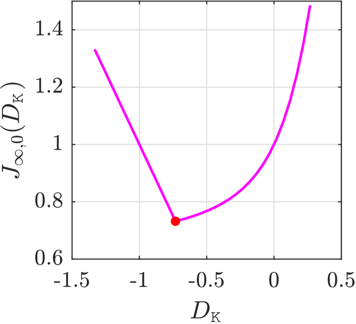
(a) $a=-1,D_{\mathsf{K}}^{\star}=1-\sqrt{3}$

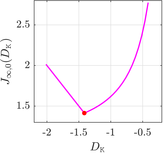
(b) $a=0,D_{\mathsf{K}}^{\star}=-\sqrt{2}$

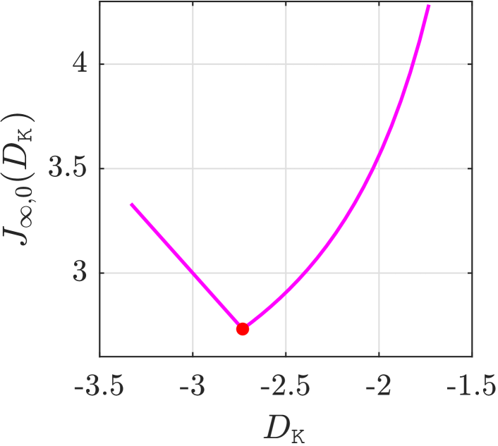
(c) $a=1,D_{\mathsf{K}}^{\star}=-1-\sqrt{3}$

Figure 9: Landscape of ${J}_{\infty,0}(D_{\mathsf{K}})$ for static output feedback $u(t)=D_{\mathsf{K}}y(t)$ in Example C.2, where the red points highlight the globally optimal policy $D_{\mathsf{K}}^{\star}$ that is a nonsmooth stationary point.

To summarize, for any $\gamma>\sqrt{a^{2}+2}+a$, the Riccati equation A.24 has stabilizing solutions C.4a and C.5 that satisfies $\rho(X_{\infty}Y_{\infty})<\gamma^{2}$. Therefore, a suboptimal $\mathcal{H}_{\infty}$ policy that ensure $J_{\infty,n}({\mathsf{K}})$ is in the form of

$$\dot{\xi}(t) =(a+\gamma^{-2}X_{\infty})\xi(t)+u(t)+(1-\gamma^{-2}Y_{\infty}X_{\infty})^{-1}Y_{\infty}(y(t)-\xi(t))$$ (C.6)

$$u(t) =-X_{\infty}\xi(t).$$

Let $\gamma\to\sqrt{a^{2}+2}+a$, we have the globally optimal $\mathcal{H}_{\infty}$ cost is $\gamma_{\mathrm{opt}}=\sqrt{a^{2}+2}+a,$ for which the optimal controller becomes a static output feedback $D_{\mathsf{K}}^{\star}=-X_{\infty}$ (see [23, Example 16.1]):

$$u(t)=-X_{\infty}y(t)=-\frac{a+\sqrt{a^{2}+1-\gamma_{\mathrm{opt}}^{-2}}}{1-\gamma_{\mathrm{opt}}^{-2}}y(t)=-\gamma_{\mathrm{opt}}y(t).$$

Thus, an optimal policy of the $\mathcal{H}_{\infty}$ robust control 15 with data C.2 is static, for all $a\in\mathbb{R}$. $\square$

Let us consider three different values $a=0,a=-1$ and $a=1$ in Example C.2. The corresponding optimal cost $\gamma_{\mathrm{opt}}$ and the optimal policies $D_{\mathsf{K}}^{\star}$ are listed as follows:

• If $a=0$, we have $\gamma_{\mathrm{opt}}=\sqrt{2}$ and $D_{\mathsf{K}}^{\star}=-\sqrt{2}$.

• If $a=-1$, we have $\gamma_{\mathrm{opt}}=\sqrt{3}-1$ and $D_{\mathsf{K}}^{\star}=1-\sqrt{3}$.

• If $a=1$, we have $\gamma_{\mathrm{opt}}=\sqrt{3}+1$ and $D_{\mathsf{K}}^{\star}=-1-\sqrt{3}$.

Figure 9 and Figure 10 illustrate the landscape of $\mathcal{H}_{\infty}$ cost for the cases of static output feedback and dynamic output feedback, i.e., $J_{\infty,0}(D_{\mathsf{K}})$ and $J_{\infty,1}({\mathsf{K}})$, respectively. In Figure 9, $J_{\infty,0}(D_{\mathsf{K}})$ is plotted as a function of $D_{\mathsf{K}}$ around the globally optimal policy $D_{\mathsf{K}}^{\star}$; in Figure 10, $J_{\infty,1}({\mathsf{K}})$ is plotted as a function of $(B_{\mathsf{K}},C_{\mathsf{K}})$ around $(0,0)$ by fixing $D_{\mathsf{K}}=D_{\mathsf{K}}^{\star}$ and $A_{\mathsf{K}}=-1$. It is clear that these $\mathcal{H}_{\infty}$ cost functions are all non-smooth (the nonsmooth points are highlighted in red).

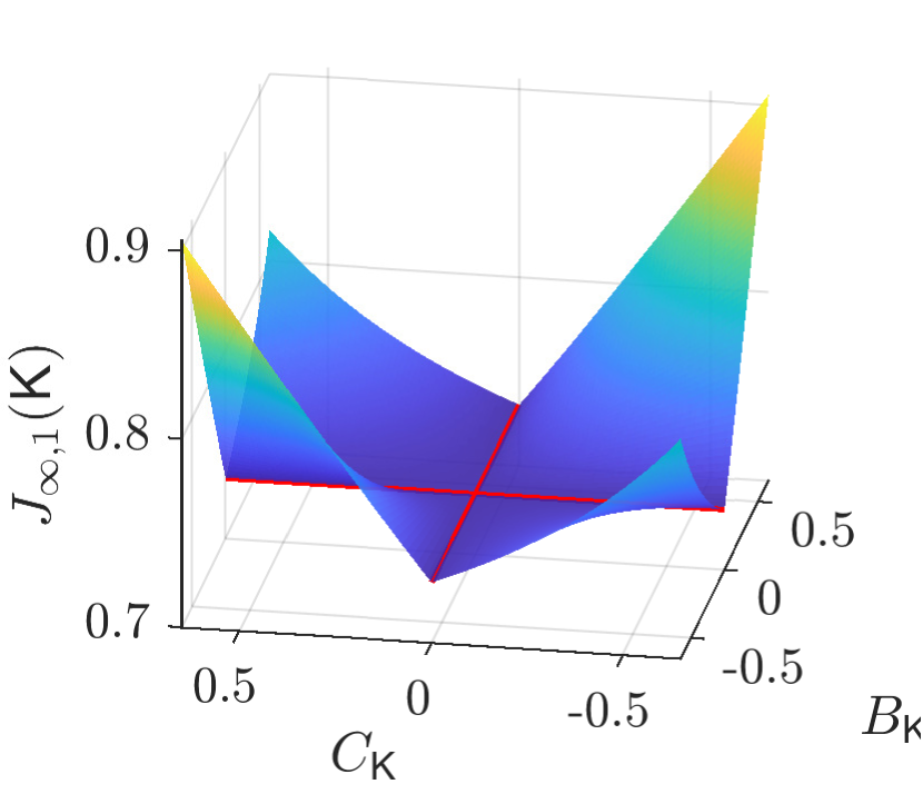
(a) $a=-1,\gamma_{\mathrm{opt}}=\sqrt{3}-1$

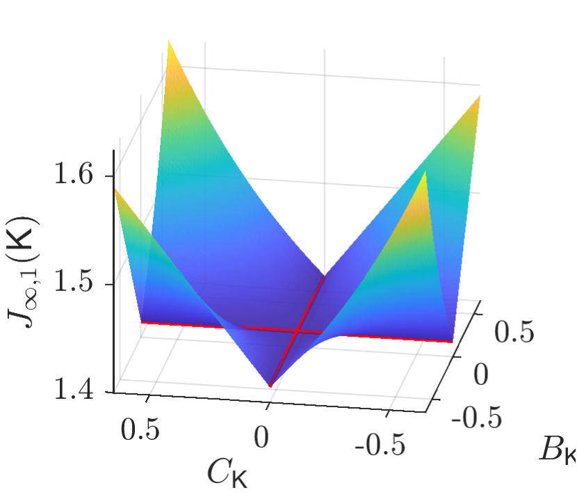
(b) $a=0,\gamma_{\mathrm{opt}}=\sqrt{2}$

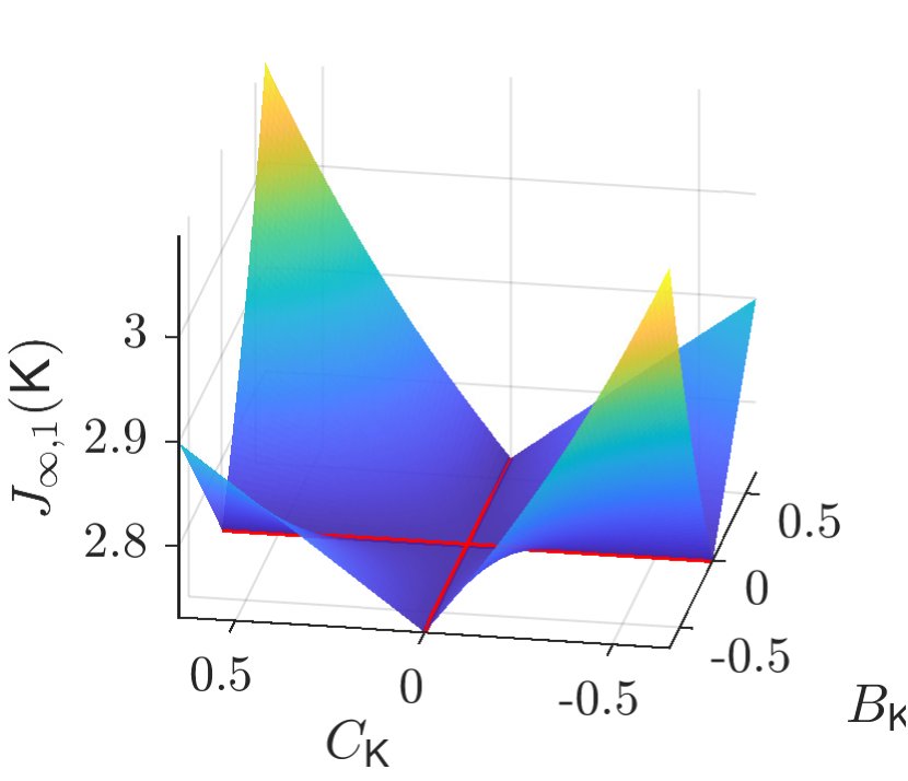
(c) $a=1,\gamma_{\mathrm{opt}}=\sqrt{3}+1$

Figure 10: Landscape of ${J}_{\infty,1}({\mathsf{K}})$ for dynamic output feedback in Example C.2, where we fix $D_{\mathsf{K}}=D_{\mathsf{K}}^{\star}$ and $A_{\mathsf{K}}=-1$ and change $B_{{\mathsf{K}}}\in(-0.6,0.6)$, $C_{{\mathsf{K}}}\in(-0.6,0.6)$. The red line highlights the nonsmooth points.

Example C.3 (Globally optimal $\mathcal{H}_{\infty}$ policies that are degenerate).

Consider the same $\mathcal{H}_{\infty}$ control instance in Example 5.1. As discussed in Example C.2, via analyzing the limiting behavior in Theorem A.2, we can show that a globally optimal $\mathcal{H}_{\infty}$ controller in this instance is achieved by a static output feedback policy

$$u(t)=D_{\mathsf{K}}^{\star}y(t),\quad\text{with}\quad D_{\mathsf{K}}^{\star}=1-\sqrt{3},$$ (C.7)

and the globally optimal $\mathcal{H}_{\infty}$ cost is $J^{\star}_{\infty,1}=\sqrt{3}-1$. One can also verify zero is an element of its Clarke subdifferential at $D_{\mathsf{K}}^{\star}$, i.e., $0\in\partial J(D_{\mathsf{K}}^{\star})$. Indeed, the closed-loop transfer function reads as

$$\mathbf{T}_{zd}(D_{\mathsf{K}}^{\star},j\omega)=\frac{1}{\sqrt{3}+j\omega}\begin{bmatrix}1&1-\sqrt{3}\\ 1-\sqrt{3}&(1-\sqrt{3})(1+j\omega)\end{bmatrix}$$

with its singular values given by

$$\sqrt{3}-1,\quad\text{and}\quad\sqrt{\frac{1}{\omega^{2}+3}}.$$

Thus we have $\sigma_{\mathrm{max}}(\mathbf{T}_{zd}(D_{\mathsf{K}}^{\star},j\omega))=\sqrt{3}-1,\forall\omega\in\mathbb{R}.$ Using the subdifferential formula given in Section B.2, one can verify that $\partial J(D_{\mathsf{K}}^{\star})$ contains a positive subgradient $\approx 0.0359$ for $\omega=0.3$, and a negative subgradient $\approx-0.0838$ for $\omega=0.5$. The Clarke stationarity of $D_{\mathsf{K}}^{\star}$ follows from the convexity of the subdifferential.

We now discuss different state-space realizations of this globally optimal controller C.7.

• Uncontrollable and unobservable cases: For any $a<0$, the following uncontrollable and unobservable policy

  $$A_{\mathsf{K}}=a,\quad B_{\mathsf{K}}=0,\quad C_{\mathsf{K}}=0,\quad D_{\mathsf{K}}^{\star}=1-\sqrt{3},$$ (C.8)

  is also globally optimal. The closed-loop system matrices with C.8 read as

  $$A_{\mathrm{cl}}=\begin{bmatrix}-\sqrt{3}&0\\ 0&a\end{bmatrix},\quad B_{\mathrm{cl}}=\begin{bmatrix}1&1-\sqrt{3}\\ 0&0\end{bmatrix},\quad C_{\mathrm{cl}}=\begin{bmatrix}1&0\\ 1-\sqrt{3}&0\end{bmatrix},\quad D_{\mathrm{cl}}=\begin{bmatrix}0&0\\ 0&1-\sqrt{3}\end{bmatrix}.$$

  Then, 25a with $\gamma=\sqrt{3}-1$ is equivalent to

  $$\begin{bmatrix}2\begin{bmatrix}-\sqrt{3}&0\\ 0&a\end{bmatrix}\begin{bmatrix}p_{1}&p_{2}\\ p_{2}&p_{3}\end{bmatrix}&\begin{bmatrix}p_{1}&p_{2}\\ p_{2}&p_{3}\end{bmatrix}\begin{bmatrix}1&1-\sqrt{3}\\ 0&0\end{bmatrix}\\ *&-(\sqrt{3}-1)^{2}\begin{bmatrix}1&0\\ 0&1\end{bmatrix}\end{bmatrix}+\begin{bmatrix}\begin{bmatrix}1+(1-\sqrt{3})^{2}&0\\ 0&0\end{bmatrix}&\begin{bmatrix}0&(1-\sqrt{3})^{2}\\ 0&0\end{bmatrix}\\ *&\begin{bmatrix}0&0\\ 0&(1-\sqrt{3})^{2}\end{bmatrix}\end{bmatrix}\preceq 0,$$

  which is the same as

  $$\begin{bmatrix}1+(1-\sqrt{3})^{2}-2\sqrt{3}p_{1}&ap_{2}-\sqrt{3}p_{2}&p_{1}&p_{1}(1-\sqrt{3})+(1-\sqrt{3})^{2}\\ *&2ap_{3}&p_{2}&p_{2}(1-\sqrt{3})\\ *&*&-(\sqrt{3}-1)^{2}&0\\ *&*&*&0\end{bmatrix}\preceq 0.$$

  Since the (4,4) element is zero, the entire column must be zero, i.e., $p_{2}=0,\,p_{1}=\sqrt{3}-1.$ Then the LMI is simplified as

  $$\begin{bmatrix}-1&0&\sqrt{3}-1&0\\ *&2ap_{3}&0&0\\ *&*&-(\sqrt{3}-1)^{2}&0\\ *&*&*&0\end{bmatrix}\preceq 0,$$

  which is satisfied for any $p_{3}\geq 0$ since $a<0$.

  Since we always have $p_{2}=0$, this policy C.8 is degenerate.

• Controllable but unobservable cases: For any $a<0,b\neq 0$, the following controllable but unobservable policy

  $$A_{\mathsf{K}}=a,\quad B_{\mathsf{K}}=b,\quad C_{\mathsf{K}}=0,\quad D_{\mathsf{K}}^{\star}=1-\sqrt{3},$$ (C.9)

  is also globally optimal. The closed-loop system matrices with C.8 read as

  $$A_{\mathrm{cl}}=\begin{bmatrix}-\sqrt{3}&0\\ b&a\end{bmatrix},\quad B_{\mathrm{cl}}=\begin{bmatrix}1&1-\sqrt{3}\\ 0&b\end{bmatrix},\quad C_{\mathrm{cl}}=\begin{bmatrix}1&0\\ 1-\sqrt{3}&0\end{bmatrix},\quad D_{\mathrm{cl}}=\begin{bmatrix}0&0\\ 0&1-\sqrt{3}\end{bmatrix}.$$

  Then, 25a with $\gamma=\sqrt{3}-1$ is equivalent to

  $$\begin{bmatrix}\begin{bmatrix}-\sqrt{3}&0\\ b&a\end{bmatrix}\begin{bmatrix}p_{1}&p_{2}\\ p_{2}&p_{3}\end{bmatrix}+*&\begin{bmatrix}p_{1}&p_{2}\\ p_{2}&p_{3}\end{bmatrix}\begin{bmatrix}1&1-\sqrt{3}\\ 0&b\end{bmatrix}\\ *&-(\sqrt{3}-1)^{2}\begin{bmatrix}1&0\\ 0&1\end{bmatrix}\end{bmatrix}+\begin{bmatrix}\begin{bmatrix}1+(1-\sqrt{3})^{2}&0\\ 0&0\end{bmatrix}&\begin{bmatrix}0&(1-\sqrt{3})^{2}\\ 0&0\end{bmatrix}\\ *&\begin{bmatrix}0&0\\ 0&(1-\sqrt{3})^{2}\end{bmatrix}\end{bmatrix}\preceq 0,$$

  which is the same as

  $$\begin{bmatrix}1+(1-\sqrt{3})^{2}-2\sqrt{3}p_{1}+2bp_{2}&ap_{2}-\sqrt{3}p_{2}+bp_{3}&p_{1}&p_{1}(1-\sqrt{3})+bp_{2}+(1-\sqrt{3})^{2}\\ *&2ap_{3}&p_{2}&p_{2}(1-\sqrt{3})+bp_{3}\\ *&*&-(\sqrt{3}-1)^{2}&0\\ *&*&*&0\end{bmatrix}\preceq 0.$$

  Since the (4,4) element is zero, we must have

  $$\begin{cases}p_{2}(1-\sqrt{3})+bp_{3}&=0,\\ p_{1}(1-\sqrt{3})+bp_{2}+(1-\sqrt{3})^{2}&=0,\end{cases}\quad\Rightarrow\quad\begin{cases}p_{3}&=\displaystyle\frac{\sqrt{3}-1}{b}p_{2},\\ p_{1}&=\displaystyle\frac{b}{\sqrt{3}-1}p_{2}+\sqrt{3}-1.\end{cases}$$

  Then, the LMI is simplified as

  $$\begin{bmatrix}-1+\displaystyle\frac{2bp_{2}}{1-\sqrt{3}}&(a-1)p_{2}&\displaystyle\frac{b}{\sqrt{3}-1}p_{2}+\sqrt{3}-1&0\\ *&\displaystyle\frac{2a(\sqrt{3}-1)}{b}p_{2}&p_{2}&0\\ *&*&-(\sqrt{3}-1)^{2}&0\\ *&*&*&0\end{bmatrix}\preceq 0.$$

  The determinant of the 3-by-3 non-zero block is

  $$p_{2}^{2}\times\big{(}(4-2\sqrt{3})a^{2}+(10-6\sqrt{3})a+7-4\sqrt{3}\big{)}$$

  $$= p_{2}^{2}\times(4-2\sqrt{3})\left(a-\frac{\sqrt{3}-1}{2}\right)^{2}$$

  $$\leq 0.$$

  Therefore, we must have $p_{2}=0$ since $a<0$.

  In summary, for the controllable but unobservable policy C.9, the LMI 25a with $\gamma=\sqrt{3}-1$ admits a unique positive semidefinite solution

  $$P=\begin{bmatrix}\sqrt{3}-1&0\\ 0&0\end{bmatrix}\succeq 0.$$

  Thus, this policy C.9 is degenerate.

• Uncontrollable but observable cases: For any $a<0,c\neq 0$, the following uncontrollable but observable policy

  $$A_{\mathsf{K}}=a,\quad B_{\mathsf{K}}=0,\quad C_{\mathsf{K}}=c,\quad D_{\mathsf{K}}^{\star}=1-\sqrt{3},$$ (C.10)

  is also globally optimal. The closed-loop system matrices with C.10 read as

  $$A_{\mathrm{cl}}=\begin{bmatrix}-\sqrt{3}&c\\ 0&a\end{bmatrix},\quad B_{\mathrm{cl}}=\begin{bmatrix}1&1-\sqrt{3}\\ 0&0\end{bmatrix},\quad C_{\mathrm{cl}}=\begin{bmatrix}1&0\\ 1-\sqrt{3}&c\end{bmatrix},\quad D_{\mathrm{cl}}=\begin{bmatrix}0&0\\ 0&1-\sqrt{3}\end{bmatrix}.$$

  Then, 25a with $\gamma=\sqrt{3}-1$ is equivalent to

  $$\begin{bmatrix}\begin{bmatrix}-\sqrt{3}&c\\ 0&a\end{bmatrix}\begin{bmatrix}p_{1}&p_{2}\\ p_{2}&p_{3}\end{bmatrix}+*&\begin{bmatrix}p_{1}&p_{2}\\ p_{2}&p_{3}\end{bmatrix}\begin{bmatrix}1&1-\sqrt{3}\\ 0&0\end{bmatrix}\\ *&-(\sqrt{3}-1)^{2}\begin{bmatrix}1&0\\ 0&1\end{bmatrix}\end{bmatrix}+\begin{bmatrix}\begin{bmatrix}1+(1-\sqrt{3})^{2}&c(1-\sqrt{3})\\ *&c^{2}\end{bmatrix}&\begin{bmatrix}0&(1-\sqrt{3})^{2}\\ 0&c(1-\sqrt{3}\end{bmatrix}\\ *&\begin{bmatrix}0&0\\ 0&(1-\sqrt{3})^{2}\end{bmatrix}\end{bmatrix}\preceq 0,$$

  which is the same as

  $$\begin{bmatrix}1+(1-\sqrt{3})^{2}-2\sqrt{3}p_{1}&(a-\sqrt{3})p_{2}+c(p_{1}+1-\sqrt{3})&p_{1}&(\sqrt{3}-1)^{2}-p_{1}(\sqrt{3}-1)\\ *&c^{2}+2(ap_{3}+cp_{2})&p_{2}&(p_{2}+c)(1-\sqrt{3})\\ *&*&-(\sqrt{3}-1)^{2}&0\\ *&*&*&0\end{bmatrix}\preceq 0.$$

  Similarly, we must have $p_{2}=-c,\quad p_{1}=\sqrt{3}-1.$ The LMI is simplified as

  $$\begin{bmatrix}-1&(\sqrt{3}-a)c&\sqrt{3}-1&0\\ *&2ap_{3}-c^{2}&-c&0\\ *&*&-(\sqrt{3}-1)^{2}&0\\ *&*&*&0\end{bmatrix}\preceq 0.$$

  The determinant of the 3-by-3 nonzero block is (recall that $a<0$)

  $$c^{2}((4-2\sqrt{3})a^{2}+(10-6\sqrt{3})a+7-4\sqrt{3})$$

  $$= c^{2}\times(4-2\sqrt{3})\left(a-\frac{\sqrt{3}-1}{2}\right)^{2}\leq 0$$

  which can not be feasible unless $c=0$. In summary, for the uncontrollable but observable policy C.10, the LMI 25a with $\gamma=\sqrt{3}-1$ is infeasible. Thus, this policy C.10 is also degenerate.

To conclude this example, we have verified that all the following state-space realizations of the static optimal policy C.7

$$A_{\mathsf{K}} =a,\quad B_{\mathsf{K}}=b,\quad C_{\mathsf{K}}=0,\quad D_{\mathsf{K}}=1-\sqrt{3}$$

$$A_{\mathsf{K}} =a,\quad B_{\mathsf{K}}=0,\quad C_{\mathsf{K}}=c,\quad D_{\mathsf{K}}=1-\sqrt{3}$$

with $a<0,b\neq 0,c\neq 0$ are all globally optimal and degenerate for the $\mathcal{H}_{\infty}$ instance Example 5.1. ∎

C.3 Boundary behavior of $\mathcal{H}_{\infty}$ cost

We here give a few more details regarding the boundary behavior of the $\mathcal{H}_{\infty}$ case in Example 5.2. In particular, we consider two cases: 1) case 1: we have a sequence of stabilizing policies that approach to a boundary point, but the corresponding $\mathcal{H}_{\infty}$ costs converge to a finite value; 2) case 2: we have another sequence of stabilizing policies that approach to the same boundary point, but the corresponding $\mathcal{H}_{\infty}$ values diverge to infinity.

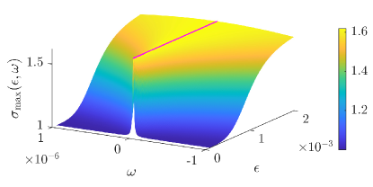
Figure 11: The shape of $\sigma_{\mathrm{max}}(\mathbf{T}_{zd}({\mathsf{K}}_{\epsilon}^{(1)},j\omega))$ in C.13. The red line denotes the maximum for small $\epsilon$, which is achieved in $\omega=0$.

Case 1: Let us first consider a sequence of parameterized stabilizing policies of the form

$${\mathsf{K}}_{\epsilon}^{(1)}=\begin{bmatrix}0&\epsilon\\ -\epsilon&0\end{bmatrix}\in\mathcal{C}_{1},\quad\forall\epsilon\neq 0,$$ (C.11)

which is the same as 36a in the main text. The corresponding closed-loop transfer function from $d(t)$ to $z(t)$ become

$$\mathbf{T}_{zd}({\mathsf{K}}_{\epsilon}^{(1)},s)=\frac{1}{s^{2}+s+\epsilon}\begin{bmatrix}s&-\epsilon^{2}\\ -\epsilon^{2}&-\epsilon^{2}(s+1)\end{bmatrix}.$$

Using the following closed-form formula for the maximum singular value of a $2\times 2$ matrix $\mathbf{T}_{zd}$:

$$\sigma_{\mathrm{max}}(\mathbf{T}_{zd})=\left(\frac{\mathrm{tr}(\mathbf{T}_{zd}^{{\mathsf{H}}}\mathbf{T}_{zd})+\sqrt{\mathrm{tr}(\mathbf{T}_{zd}^{{\mathsf{H}}}\mathbf{T}_{zd})^{2}-4\mathrm{det}(\mathbf{T}_{zd}^{{\mathsf{H}}}\mathbf{T}_{zd})}}{2}\right)^{1/2},$$ (C.12)

the maximum singular value of $\mathbf{T}_{zd}({\mathsf{K}}_{\epsilon}^{(1)},j\omega)$ reads as

$$\sigma^{2}_{\mathrm{max}}(\mathbf{T}_{zd}({\mathsf{K}}_{\epsilon}^{(1)},j\omega))=\frac{(\epsilon^{4}+1)\omega^{2}+3\epsilon^{4}+\sqrt{(\epsilon^{8}-2\epsilon^{4}+1)\omega^{4}+(6\epsilon^{8}+8\epsilon^{6}+2\epsilon^{4})\omega^{2}+5\epsilon^{8}}}{2\omega^{4}+(2-4\epsilon^{2})\omega^{2}+2\epsilon^{4}}.$$ (C.13)

For this function $\sigma_{\mathrm{max}}(\mathbf{T}_{zd}({\mathsf{K}}_{\epsilon}^{(1)},j\omega))$, its behavior for small $\epsilon$ is is shown in Figure 11. Indeed, we claim the result in Fact C.1. Therefore, we have

$$\lim_{\epsilon\downarrow 0}J_{\infty,1}({\mathsf{K}}_{\epsilon}^{(1)}) =\lim_{\epsilon\downarrow 0,\epsilon\leq\epsilon_{0}}\left(\frac{3\epsilon^{4}+\sqrt{5\epsilon^{8}}}{2\epsilon^{4}}\right)^{1/2}=\left(\frac{3+\sqrt{5}}{2}\right)^{1/2}=\frac{1+\sqrt{5}}{2},$$

which confirms the statement of finite value in Example 5.2.

Fact C.1.

Consider the sequence of stabilizing policies C.11. The $\mathcal{H}_{\infty}$ cost of ${\mathsf{K}}_{\epsilon}^{(1)}$, defined as

$$J_{\infty,1}({\mathsf{K}}_{\epsilon}^{(1)})=\sup_{\omega\in\mathbb{R}}\sigma_{\mathrm{max}}(\mathbf{T}_{zd}({\mathsf{K}}_{\epsilon}^{(1)},j\omega))$$

is achieved at $\omega=0$ when $0<\epsilon<\epsilon_{0}$ for sufficiently small $\epsilon_{0}>0$.

Proof: From C.13, for notational simplicity, let us choose $x=\omega^{2}$ and define

$$f(x)= \frac{(\epsilon^{4}+1)x+3\epsilon^{4}+\sqrt{(\epsilon^{8}-2\epsilon^{4}+1)x^{2}+2\epsilon^{4}(3\epsilon^{4}+4\epsilon^{2}+1)x+5\epsilon^{8}}}{2x^{2}+(2-4\epsilon^{2})x+2\epsilon^{4}}=\sigma_{\mathrm{max}}^{2}\left(\mathbf{T}_{zd}({\mathsf{K}}_{\epsilon}^{(1)},j\omega)\right).$$

We can prove that when $\epsilon>0$ is small enough, $f(x)$ is a monotonically non-increasing function, i.e.

$$f^{\prime}(x)\leq 0,\qquad\forall x\geq 0.$$ (C.14)

Indeed, to verify C.14, let us write $f(x)=f_{1}(x)+f_{2}(x)$ with

$$f_{1}(x) =\frac{(\epsilon^{4}+1)x+3\epsilon^{4}}{2x^{2}+(2-4\epsilon^{2})x+2\epsilon^{4}}=\frac{p_{1}(x)}{q_{1}(x)},$$

$$f_{2}(x) =\frac{\sqrt{(\epsilon^{8}-2\epsilon^{4}+1)x^{2}+2\epsilon^{4}(3\epsilon^{4}+4\epsilon^{2}+1)x+5\epsilon^{8}}}{2x^{2}+(2-4\epsilon^{2})x+2\epsilon^{4}}=\frac{p_{2}(x)}{q_{2}(x)}.$$

Then, there exists an $\epsilon_{0}>0$ such that $f_{1}(x)$ is a monotonically decreasing function, i.e.,

$$p_{1}^{\prime}(x)q_{1}(x)-p_{1}(x)q_{1}^{\prime}(x) =2\epsilon^{8}+12\epsilon^{6}-2\epsilon^{4}(x^{2}+6x+2)-x^{2}$$

$$\leq 2\epsilon^{8}+12\epsilon^{6}-4\epsilon^{4}-x^{2}$$

$$<0,\qquad\forall x\geq 0,\epsilon\leq\epsilon_{0}.$$

Similarly, we can verify that $f_{2}(x)$ is also monotonically decreasing when $\epsilon$ is sufficiently small. Thus, the maximum of $f(x)$ is achieved at $x=0$: there exists a sufficiently small $\epsilon_{0}>0$ such that

$$J_{\infty,1}^{2}({\mathsf{K}}_{\epsilon}^{(1)})=\max_{x}\;f(x)=f(0)=\frac{3\epsilon^{4}+\sqrt{5\epsilon^{8}}}{2\epsilon^{4}}=\left(\frac{1+\sqrt{5}}{2}\right)^{2},\qquad\text{if }\;\epsilon\leq\epsilon_{0}.$$

Case 2: We next consider another sequence of parameterized dynamic policies of the form

$${\mathsf{K}}_{\epsilon}^{(2)}=\begin{bmatrix}0&\epsilon+\epsilon^{d}\\ -\epsilon&\epsilon^{2}\end{bmatrix}\in\mathcal{C}_{1},\quad\forall 1>\epsilon>0$$ (C.15)

where $d>0$ is a positive integer. When $d=4$, this policy C.15 is the same as 36b in the main text. The corresponding closed-loop transfer function from $d(t)$ to $z(t)$ is

$$\mathbf{T}_{zd}({\mathsf{K}}_{\epsilon}^{(2)},s)=\frac{1}{s^{2}+(1-\epsilon^{2})s+\epsilon^{d+1}}\begin{bmatrix}s-\epsilon^{2}&-\epsilon^{2}-\epsilon^{d+1}\\ -\epsilon^{2}-\epsilon^{d+1}&-(\epsilon^{2}+\epsilon^{d+1})(s+1)\end{bmatrix}.$$

Using C.12 we obtain its maximum singular value

$$\sigma_{\mathrm{max}}(\mathbf{T}_{zd}({\mathsf{K}}_{\epsilon}^{(2)},j\omega))=\left(\frac{\mathrm{tr}(\mathbf{T}_{zd}^{{\mathsf{H}}}\mathbf{T}_{zd})+\sqrt{\mathrm{tr}(\mathbf{T}_{zd}^{{\mathsf{H}}}\mathbf{T}_{zd})^{2}-4\mathrm{det}(\mathbf{T}_{zd}^{{\mathsf{H}}}\mathbf{T}_{zd})}}{2}\right)^{1/2},$$

where

$$\mathrm{tr}(\mathbf{T}_{zd}^{{\mathsf{H}}}\mathbf{T}_{zd})=\frac{\epsilon^{2d+2}\omega^{2}+6\epsilon^{d+3}+2\epsilon^{d+3}\omega^{2}+4\epsilon^{4}+\omega^{2}+3\epsilon^{2d+2}+\epsilon^{4}\omega^{2}}{\omega^{2}-2\epsilon^{d+1}\omega^{2}+\omega^{4}+\epsilon^{2d+2}-2\epsilon^{2}\omega^{2}+\epsilon^{4}\omega^{2}},$$

$$\mathrm{det}(\mathbf{T}_{zd}^{{\mathsf{H}}}\mathbf{T}_{zd})=\frac{\epsilon^{2}(\epsilon+\epsilon^{d})^{2}}{\omega^{2}-2\epsilon^{d+1}\omega^{2}+\omega^{4}+\epsilon^{2d+2}-2\epsilon^{2}\omega^{2}+\epsilon^{4}\omega^{2}}.$$

We find that it is tedious to evaluate the $\mathcal{H}_{\infty}$ norms $J_{\infty,1}({\mathsf{K}}_{2}(\epsilon))=\sup_{\omega\in\mathbb{R}}\,\sigma_{\mathrm{max}}(\mathbf{T}_{zd}({\mathsf{K}}_{\epsilon}^{(2)},j\omega))$ analytically. Instead, our numerical simulation in Figure 12 suggests that for $d\geq 3$, we have

$$J_{\infty,1}({\mathsf{K}}_{2}(\epsilon))=\sup_{\omega\in\mathbb{R}}\,\sigma_{\mathrm{max}}(\mathbf{T}_{zd}(j\omega,{\mathsf{K}}_{2}(\epsilon)))\approx\frac{2}{\epsilon^{d-1}}\qquad\text{if}\;\;0<\epsilon\leq 10^{-1}.$$ (C.16)

Thus, the corresponding $\mathcal{H}_{\infty}$ performance for C.15 will go to infinity as $\epsilon\to 0$ (i.e., the sequence of the policies goes to the boundary). Note that the dynamic policies in C.11 and C.15 go to the same boundary point when $\epsilon\to 0$.

Figure 12: Numerical $\mathcal{H}_{\infty}$ norms for the policies C.15: the dots are numerical values of $\mathcal{H}_{\infty}$ norms for each point $\epsilon$, and each line represents the least square fitting from those data points, which agree with C.16.

Appendix D Technical Proofs

In this section, we provide some technical proofs that are missing in the main text.

D.1 Auxiliary technical lemmas

Define the set of stable matrices $\mathcal{S}_{n}=\{A\in\mathbb{R}^{n\times n}\mid\Re(\lambda_{i}(A))<0,i=1,\ldots,n\}$. It is not hard to see that $\partial\mathcal{S}_{n}$ consists of $n\times n$ real matrices whose set of eigenvalues has a nonempty intersection with the imaginary axis.

Lemma D.1.

Consider a sequence of stable LTI systems $\mathbf{G}_{t}=C_{t}(sI-A_{t})^{-1}B_{t}+D_{t}$ with $A_{t}\in\mathcal{S}_{n}$, $B_{t}\in\mathbb{R}^{n\times m}$, $C_{t}\in\mathbb{R}^{p\times n}$ and $D_{t}\in\mathbb{R}^{p\times m}$. Suppose $\lim_{t\to\infty}(A_{t},B_{t},C_{t},D_{t})=(\hat{A},\hat{B},\hat{C},\hat{D})$ with $\hat{A}\in\partial\mathcal{S}_{n}$, and the transfer matrix

$$\hat{\mathbf{G}}(s)=\hat{C}(sI-\hat{A})^{-1}\hat{B}+\hat{D}$$

has at least one pole that lies on the imaginary axis. Then

$$\lim_{t\rightarrow\infty}\|\mathbf{G}_{t}\|_{\mathcal{H}_{\infty}}=+\infty.$$

In addition, if $D_{t}=0$ for all $t=1,2,\ldots$, then

$$\lim_{t\rightarrow\infty}\|\mathbf{G}_{t}\|_{\mathcal{H}_{2}}=+\infty.$$

Proof.

Since one of the poles of the transfer matrix $\hat{\mathbf{G}}(s)=\hat{C}(sI-\hat{A})^{-1}\hat{B}+\hat{D}$ lies on the imaginary axis, by using the fact that each pole of $\hat{\mathbf{G}}$ must also be a pole of some entry of $\hat{\mathbf{G}}$, we see that one of the entries of $\hat{\mathbf{G}}$, say $\hat{\mathbf{G}}_{ik}$, must have a pole on the imaginary axis. We can therefore write $\hat{\mathbf{G}}_{ik}$ in the following form:

$$\hat{\mathbf{G}}_{ik}(s)=h(s)\prod_{\kappa=1}^{K}\frac{1}{(s-j\omega_{\kappa})^{m_{\kappa}}},$$

where $\omega_{\kappa}\in\mathbb{R}$ for $\kappa=1,\ldots,K$ are distinct, each $m_{\kappa}\geq 1$ is the multiplicity of $j\omega_{\kappa}$, and $h(s)$ is a rational function with no poles on the imaginary axis. Consequently,

$$|\hat{\mathbf{G}}_{ik}(j\omega)|=|h(j\omega)|\prod_{\kappa=1}^{K}\frac{1}{(\omega-\omega_{\kappa})^{m_{\kappa}}}.$$ (D.1)

Now let us consider the transfer function

$$\mathbf{G}_{t,ik}(s)=\left[C_{t}(sI-A_{t})^{-1}B_{t}+D_{t}\right]_{ik},$$

i.e., $\mathbf{G}_{t,ik}$ is the $(i,k)$’th entry of the transfer matrix $C_{t}(sI-A_{t})^{-1}B_{t}+D_{t}$. Then it’s not hard to verify by continuity that

$$\lim_{t\rightarrow\infty}\mathbf{G}_{t,ik}(s)=\hat{\mathbf{G}}_{ik}(s)$$

for every $s\in j\mathbb{R}$ that is not an eigenvalue of $A$. In other words, $\mathbf{G}_{t,ik}(j\omega)$ converges to $\hat{\mathbf{G}}_{ik}(j\omega)$ for almost every $\omega\in\mathbb{R}$.

We first show that $\lim_{t\rightarrow\infty}\|\mathbf{G}_{t}\|_{\mathcal{H}_{\infty}}=+\infty$. From the expression D.1, we can see that for any $M>0$, there exists $\omega_{M}\in\mathbb{R}$ such that $j\omega_{M}$ is not an eigenvalue of $A$ and $|\hat{\mathbf{G}}_{ik}(j\omega_{M})|\geq 2M$. Then since $\lim_{t\rightarrow}\mathbf{G}_{t,ik}(j\omega_{M})=\hat{\mathbf{G}}_{ik}(j\omega_{M})$, we can find $T\in\mathbb{N}$ such that for all $t\geq T$, we have

$$|\mathbf{G}_{t,ik}(j\omega_{M})|\geq M.$$

We also have

$$\|\mathbf{G}_{t}\|_{\mathcal{H}_{\infty}}\geq\sigma_{\max}(\mathbf{G}_{t}(j\omega_{M}))\geq|\mathbf{G}_{t,ik}(j\omega_{M})|.$$

Summarizing the previous results, we see that for any $M>0$, there exists $T\in\mathbb{N}$ such that for all $t\geq T$, we have $\|\mathbf{G}_{t}\|_{\mathcal{H}_{\infty}}\geq M$. Therefore $\lim_{t\rightarrow\infty}\|\mathbf{G}_{t}\|_{\mathcal{H}_{\infty}}=+\infty$.

Now suppose $D_{t}=0$ for each $t$. To show that $\|\mathbf{G}_{t}\|_{\mathcal{H}_{2}}\rightarrow+\infty$, we note that

$$\|\mathbf{G}_{t}\|_{\mathcal{H}_{2}}^{2}={} \frac{1}{2\pi}\int_{-\infty}^{+\infty}\operatorname{trace}(\mathbf{G}_{t}(j\omega)^{{\mathsf{H}}}\mathbf{G}_{t}(j\omega))\,d\omega\geq{}\frac{1}{2\pi}\int_{-\infty}^{+\infty}|\mathbf{G}_{t,ik}(j\omega)|^{2}\,d\omega.$$

Therefore

$$\liminf_{t\rightarrow\infty}\|\mathbf{G}_{t}\|_{\mathcal{H}_{2}}^{2}\geq{} \frac{1}{2\pi}\liminf_{t\rightarrow\infty}\int_{-\infty}^{+\infty}|\mathbf{G}_{t,ik}(j\omega)|^{2}\,d\omega$$

$$\geq{} \frac{1}{2\pi}\int_{-\infty}^{+\infty}\liminf_{t\rightarrow\infty}|\mathbf{G}_{t,ik}(j\omega)|^{2}\,d\omega$$

$$={} \frac{1}{2\pi}\int_{-\infty}^{+\infty}|\hat{\mathbf{G}}_{ik}(j\omega)|^{2}\,d\omega$$

$$={} \frac{1}{2\pi}\int_{-\infty}^{+\infty}|h(j\omega)|^{2}\prod_{\kappa=1}^{K}\frac{1}{(\omega-\omega_{\kappa})^{2m_{\kappa}}}\,d\omega=+\infty,$$

where in the second step we used Fatou’s lemma [93, Theorem 1.17]. We can then conclude $\|\mathbf{G}_{t}\|_{\mathcal{H}_{2}}\rightarrow+\infty$. ∎

Combining Lemma D.1 with Lemma A.10 and using the fact that the poles of the transfer matrix of a controllable and observable system $(\hat{A},\hat{B},\hat{C},\hat{D})$ are exactly the same as the eigenvalues of $\hat{A}$ (see e.g., [23, Section 3.11]), we get the following corollary:

Corollary D.1.

Consider a sequence $({\mathsf{K}}_{t})_{t=1}^{\infty}$ in $\mathcal{C}_{n}$. Suppose $\lim_{t\to\infty}{\mathsf{K}}_{t}={\mathsf{K}}_{\infty}$ for some ${\mathsf{K}}_{\infty}\in\partial\mathcal{C}_{n}$ that is controllable and observable, then

$$\lim_{t\rightarrow\infty}J_{\infty,n}({\mathsf{K}}_{t})=+\infty.$$

In addition, if $D_{{\mathsf{K}}_{t}}=0$ for all $t=1,2,\ldots$, then

$$\lim_{t\rightarrow\infty}J_{\mathtt{LQG},n}({\mathsf{K}}_{t})=+\infty.$$

D.2 Proof of Theorem 3.1

Part I. Sufficiency.

We start our proof of sufficiency from the following fact about positive semidefinite matrices.

Fact D.1.

Given a positive semidefinite block matrix as

$$\begin{bmatrix}A&B\\ B^{{\mathsf{T}}}&C\end{bmatrix}\in\mathbb{S}^{n+n}_{+},$$

if $B\in\mathbb{R}^{n\times n}$ is full rank, then both $A$ and $C$ are strictly positive definite.

Proof of Fact D.1.

Suppose $A$ is only positive semidefinite with a zero eigenvalue. Let $x_{1}\neq 0$ be the eigenvector, i.e., $Ax_{1}=0$. Then for all $x_{2}\in\mathbb{R}^{n}$, we have

$$\begin{bmatrix}x_{1}\\ x_{2}\end{bmatrix}^{{\mathsf{T}}}\begin{bmatrix}A&B\\ B^{{\mathsf{T}}}&C\end{bmatrix}\begin{bmatrix}x_{1}\\ x_{2}\end{bmatrix}=2x_{1}^{{\mathsf{T}}}Bx_{2}+x_{2}^{{\mathsf{T}}}Cx_{2}\geq 0.$$ (D.2)

Since $B$ is full rank, we can find a vector $x_{2}$ such that $x_{1}^{{\mathsf{T}}}Bx_{2}<0$ (e.g., $x_{2}=-B^{-1}x_{1}/\|x_{1}\|$). The first term in D.2 can be made arbitrarily below zero when we fix $x_{2}$ and scale $x_{1}$, making D.2 invalid. Thus $A$ must be positive definite. Similarly, we can show $C$ is strictly positive definite. Note that, we cannot guarantee the whole matrix is positive definite, for example $\begin{bmatrix}1&1\\ 1&1\end{bmatrix}.$ ∎

We are now ready to prove the sufficiency part of Theorem 3.1. As alluded to in the main text, the proof follows three steps:

1. The full rank of $X_{{\mathsf{K}},12}$ implies that $(A_{\mathsf{K}},B_{{\mathsf{K}}})$ is controllable, and thus $X_{{\mathsf{K}}}$ from 13a is positive definite.

2. $X_{{\mathsf{K}}}$ is thus invertible, and we construct $P=\gamma X_{{\mathsf{K}}}^{-1}$ with $\gamma=J_{\texttt{LQG},n}({\mathsf{K}})$. We show this construction satisfies 21a and 21b.

3. Further $P_{12}=\gamma(X_{{\mathsf{K}}}^{-1})_{12}$ is invertible since $X_{{\mathsf{K}},12}$ is.

The three points above confirm that ${\mathsf{K}}\in{\mathcal{C}}_{\mathrm{nd},0}$ by the definition 23. We here provide the details.

• For point 1), let ${\mathsf{K}}\in{\mathcal{C}}_{n,0}$ be an informative policy, and $X_{\mathsf{K}}$ be the corresponding solution to 13a. Then, $X_{\mathsf{K}}$ is positive semidefinite by Lemma A.2. Upon partitioning $X_{\mathsf{K}}$ as 24, since $X_{{\mathsf{K}},12}$ is full rank and $X_{{\mathsf{K}}}\succeq 0$, we must have $X_{{\mathsf{K}},22}\succ 0$ (cf. Fact D.1).

  Meanwhile, the bottom-right block of the equation 13a reads as

  $$B_{\mathsf{K}}CX_{{\mathsf{K}},12}+A_{{\mathsf{K}}}X_{{\mathsf{K}},22}+(B_{\mathsf{K}}CX_{{\mathsf{K}},12}+A_{{\mathsf{K}}}X_{{\mathsf{K}},22})^{{\mathsf{T}}}+B_{\mathsf{K}}VB_{\mathsf{K}}^{{\mathsf{T}}}=0,$$

  which is the same as

  $$(A_{{\mathsf{K}}}+B_{\mathsf{K}}CX_{{\mathsf{K}},12}X_{{\mathsf{K}},22}^{-1})X_{{\mathsf{K}},22}+X_{{\mathsf{K}},22}(A_{{\mathsf{K}}}+B_{\mathsf{K}}CX_{{\mathsf{K}},12}X_{{\mathsf{K}},22}^{-1})^{{\mathsf{T}}}+B_{\mathsf{K}}VB_{\mathsf{K}}^{{\mathsf{T}}}=0.$$

  By Lemma A.4, we know $A_{{\mathsf{K}}}+B_{\mathsf{K}}CX_{{\mathsf{K}},12}X_{{\mathsf{K}},22}^{-1}$ is stable. Since $X_{{\mathsf{K}},22}\succ 0$, Lemma A.2 further ensures that

  $$(A_{{\mathsf{K}}}+B_{\mathsf{K}}CX_{{\mathsf{K}},12}X_{{\mathsf{K}},22}^{-1},B_{\mathsf{K}}V^{1/2})$$

  is controllable, which is the same as $(A_{\mathsf{K}},B_{\mathsf{K}})$ being controllable (since controllability is invariant with state feedback; cf. Lemma A.1). Therefore, the solution $X_{{\mathsf{K}}}$ to 13a is strictly positive definite, as confirmed in [13, Lemma 4.5].

• For point 2), since $X_{\mathsf{K}}\succ 0$, the construction $P=\gamma X_{{\mathsf{K}}}^{-1}$ with $\gamma=J_{\texttt{LQG},n}({\mathsf{K}})$ is well-defined. Following the exactly same argument in Section A.3.1 (especially the logic between A.11 and A.12), this construction satisfies 21a and 21b.

• For point 3), we have the following observation

  $$PX_{\mathsf{K}}=\begin{bmatrix}P_{11}&P_{12}\\ P_{12}^{{\mathsf{T}}}&P_{22}\end{bmatrix}\begin{bmatrix}X_{{\mathsf{K}},11}&X_{{\mathsf{K}},12}\\ X_{{\mathsf{K}},12}^{{\mathsf{T}}}&X_{{\mathsf{K}},22}\end{bmatrix}=\begin{bmatrix}\gamma I&0\\ 0&\gamma I\end{bmatrix}\quad\Rightarrow\quad P_{11}X_{{\mathsf{K}},12}+P_{12}X_{{\mathsf{K}},22}=0.$$

  We know $P_{11}\succ 0,X_{{\mathsf{K}},22}\succ 0$ since $P\succ 0,X_{\mathsf{K}}\succ 0$. Then $P_{12}$ being invertible follows from the fact that $X_{{\mathsf{K}},12}$ is invertible.

This completes our proof of the sufficiency part.

Part II. Necessity.

Suppose ${\mathsf{K}}\in{\mathcal{C}}_{\mathrm{nd},0}$, and let $\gamma=J_{\mathtt{LQG},n}({\mathsf{K}})>0$. Then there exist $P\succ 0$ with $P_{12}\in\mathrm{GL}_{n}$ and $\Gamma\succeq 0$ such that

$$\begin{bmatrix}A_{\mathrm{cl}}({\mathsf{K}})^{{\mathsf{T}}}P+PA_{\mathrm{cl}}({\mathsf{K}})&PB_{\mathrm{cl}}({\mathsf{K}})\\ B_{\mathrm{cl}}({\mathsf{K}})^{{\mathsf{T}}}P&-\gamma I\end{bmatrix}\preceq 0,\quad\begin{bmatrix}P&C_{\mathrm{cl}}({\mathsf{K}})^{{\mathsf{T}}}\\ C_{\mathrm{cl}}({\mathsf{K}})&\Gamma\end{bmatrix}\succeq 0,\qquad\operatorname{tr}(\Gamma)\leq\gamma.$$

Let $\hat{X}=\gamma P^{-1}$. It’s not hard to see that $P_{12}\in\mathrm{GL}_{n}$ implies $\hat{X}_{12}\in\mathrm{GL}_{n}$ (see point 3) in the proof of the sufficiency part). By Lemma A.7, we also have

$$A_{\mathrm{cl}}({\mathsf{K}})\hat{X}+\hat{X}A_{\mathrm{cl}}({\mathsf{K}})^{{\mathsf{T}}}+B_{\mathrm{cl}}({\mathsf{K}})B_{\mathrm{cl}}({\mathsf{K}})^{{\mathsf{T}}}\preceq 0$$

and

$$\operatorname{tr}(C_{\mathrm{cl}}({\mathsf{K}})\hat{X}C_{\mathrm{cl}}({\mathsf{K}})^{{\mathsf{T}}})\leq\gamma^{2}.$$

As a result, there exists some $\tilde{B}\in\mathbb{R}^{{2n}\times k}$ such that

$$A_{\mathrm{cl}}({\mathsf{K}})\hat{X}+\hat{X}A_{\mathrm{cl}}({\mathsf{K}})^{{\mathsf{T}}}+B_{\mathrm{cl}}({\mathsf{K}})B_{\mathrm{cl}}({\mathsf{K}})^{{\mathsf{T}}}+\tilde{B}\tilde{B}^{{\mathsf{T}}}=0.$$

On the other hand, note that $X_{\mathsf{K}}$ is the solution to the Lyapunov equation

$$A_{\mathrm{cl}}({\mathsf{K}})X_{\mathsf{K}}+X_{\mathsf{K}}A_{\mathrm{cl}}({\mathsf{K}})^{{\mathsf{T}}}+B_{\mathrm{cl}}({\mathsf{K}})B_{\mathrm{cl}}({\mathsf{K}})=0,$$

and satisfies $\operatorname{tr}(C_{\mathrm{cl}}({\mathsf{K}})X_{\mathsf{K}}C_{\mathrm{cl}}({\mathsf{K}})^{{\mathsf{T}}})=\gamma^{2}$. Now let $\tilde{X}=\hat{X}-X_{\mathsf{K}}$, and we have

$$A_{\mathrm{cl}}({\mathsf{K}})\tilde{X}+\tilde{X}A_{\mathrm{cl}}({\mathsf{K}})+\tilde{B}\tilde{B}^{{\mathsf{T}}}=0,$$

showing that $\tilde{X}\succ 0$ or $\hat{X}\succeq X_{\mathsf{K}}$, while

$$\gamma^{2}=\operatorname{tr}(C_{\mathrm{cl}}({\mathsf{K}})X_{\mathsf{K}}C_{\mathrm{cl}}({\mathsf{K}})^{{\mathsf{T}}})\leq\operatorname{tr}(C_{\mathrm{cl}}({\mathsf{K}})\hat{X}C_{\mathrm{cl}}({\mathsf{K}})^{{\mathsf{T}}})\leq\gamma^{2},$$

showing that $\operatorname{tr}(C_{\mathrm{cl}}({\mathsf{K}})X_{\mathsf{K}}C_{\mathrm{cl}}({\mathsf{K}})^{{\mathsf{T}}})=\operatorname{tr}(C_{\mathrm{cl}}({\mathsf{K}})\hat{X}C_{\mathrm{cl}}({\mathsf{K}})^{{\mathsf{T}}})=\gamma^{2}$. Consequently,

$$\operatorname{tr}(C_{\mathrm{cl}}({\mathsf{K}})\tilde{X}C_{\mathrm{cl}}({\mathsf{K}})^{{\mathsf{T}}})=0.$$

By plugging $\tilde{X}=\int_{0}^{+\infty}e^{A_{\mathrm{cl}}({\mathsf{K}})\tau}\tilde{B}\tilde{B}^{{\mathsf{T}}}e^{A_{\mathrm{cl}}({\mathsf{K}})^{{\mathsf{T}}}\tau}\,d\tau$ into the above equality, we get

$$0={} \int_{0}^{+\infty}\operatorname{tr}\left(C_{\mathrm{cl}}({\mathsf{K}})e^{A_{\mathrm{cl}}({\mathsf{K}})\tau}\tilde{B}\tilde{B}^{{\mathsf{T}}}e^{A_{\mathrm{cl}}({\mathsf{K}})^{{\mathsf{T}}}\tau}C_{\mathrm{cl}}({\mathsf{K}})^{{\mathsf{T}}}\right)\,d\tau$$

$$={} \int_{0}^{+\infty}\left\|C_{\mathrm{cl}}({\mathsf{K}})e^{A_{\mathrm{cl}}({\mathsf{K}})\tau}\tilde{B}\right\|_{F}^{2}\,d\tau$$

which further gives

$$C_{\mathrm{cl}}({\mathsf{K}})e^{A_{\mathrm{cl}}({\mathsf{K}})\tau}\tilde{B}=0$$

for all $\tau\in[0,+\infty)$.

The following lemma is essential for our subsequent derivation.

Lemma D.2.

Suppose $(Q^{1/2},A)$ is observable, and suppose $\tilde{B}\in\mathbb{R}^{{2n}\times k}$ satisfies

$$C_{\mathrm{cl}}({\mathsf{K}})e^{A_{\mathrm{cl}}({\mathsf{K}})\tau}\tilde{B}=0$$

for all $\tau\in[0,+\infty)$. Let $\tilde{X}\in\mathbb{R}^{{2n}\times{2n}}$ be the solution to the Lyapunov equation

$$A_{\mathrm{cl}}({\mathsf{K}})X+XA_{\mathrm{cl}}({\mathsf{K}})^{{\mathsf{T}}}+\tilde{B}\tilde{B}^{{\mathsf{T}}}=0.$$

Then $\tilde{X}$ has the form

$$\tilde{X}=\begin{bmatrix}0_{n\times n}&0_{n\times n}\\ 0_{n\times n}&\tilde{X}_{22}\end{bmatrix}$$

for some $\tilde{X}_{22}\in\mathbb{R}^{n\times n}$.

Proof.

By applying Laplace transform to $C_{\mathrm{cl}}({\mathsf{K}})e^{A_{\mathrm{cl}}({\mathsf{K}})\tau}\tilde{B}=0$, we obtain

$$C_{\mathrm{cl}}({\mathsf{K}})(sI-A_{\mathrm{cl}}({\mathsf{K}}))^{-1}\tilde{B}=0$$ (D.3)

for all $s\in\mathbb{C}$ with $\operatorname{Re}[s]\geq 0$. To further derive implications from this equality, we decompose $\tilde{B}$ as

$$\tilde{B}=\begin{bmatrix}\tilde{B}_{1}\\ \tilde{B}_{2}\end{bmatrix},\qquad\text{where }\tilde{B}_{1},\tilde{B}_{2}\in\mathbb{R}^{n\times k}.$$

Note that $A_{\mathrm{cl}}({\mathsf{K}})=\begin{bmatrix}A&BC_{\mathsf{K}}\\ B_{\mathsf{K}}C&A_{\mathsf{K}}\end{bmatrix}$, which gives

$$(sI-A_{\mathrm{cl}}({\mathsf{K}}))^{-1}\tilde{B}=\begin{bmatrix}sI-A&-BC_{\mathsf{K}}\\ -B_{\mathsf{K}}C&sI-A_{\mathsf{K}}\end{bmatrix}^{-1}\begin{bmatrix}\tilde{B}_{1}\\ \tilde{B}_{2}\end{bmatrix}$$

$$={} \left(\begin{bmatrix}I&0\\ -B_{\mathsf{K}}C(sI\!-\!A)^{-1}&I\end{bmatrix}\!\begin{bmatrix}sI\!-\!A&0\\ 0&sI\!-\!A_{\mathsf{K}}\!-\!B_{\mathsf{K}}\mathbf{P}(s)C_{\mathsf{K}}\end{bmatrix}\!\begin{bmatrix}I&-(sI\!-\!A)^{-1}BC_{\mathsf{K}}\\ 0&I\end{bmatrix}\right)^{\!\!-1}\!\!\begin{bmatrix}\tilde{B}_{1}\\ \tilde{B}_{2}\end{bmatrix}$$

$$={} \begin{bmatrix}I&(sI-A)^{-1}BC_{\mathsf{K}}\\ 0&I\end{bmatrix}\begin{bmatrix}sI\!-\!A&0\\ 0&sI\!-\!A_{\mathsf{K}}\!-\!B_{\mathsf{K}}\mathbf{P}(s)C_{\mathsf{K}}\end{bmatrix}^{-1}\begin{bmatrix}I&0\\ B_{\mathsf{K}}C(sI\!-\!A)^{-1}&I\end{bmatrix}\begin{bmatrix}\tilde{B}_{1}\\ \tilde{B}_{2}\end{bmatrix}$$

$$={} \begin{bmatrix}I&(sI-A)^{-1}BC_{\mathsf{K}}\\ 0&I\end{bmatrix}\begin{bmatrix}(sI-A)^{-1}\tilde{B}_{1}\\ (sI-A_{\mathsf{K}}-B_{\mathsf{K}}\mathbf{P}(s)C_{\mathsf{K}})^{-1}(B_{\mathsf{K}}C(sI-A)^{-1}\tilde{B}_{1}+\tilde{B}_{2})\end{bmatrix}$$ (D.4)

where we denote $\mathbf{P}(s)=C(sI-A)^{-1}B$. Consequently, by using $C_{\mathrm{cl}}({\mathsf{K}})=\begin{bmatrix}Q^{1/2}&0\\ 0&R^{1/2}C_{\mathsf{K}}\end{bmatrix}$, we get

$$0={} C_{\mathrm{cl}}({\mathsf{K}})(sI-A_{\mathrm{cl}}({\mathsf{K}}))^{-1}\tilde{B}$$

$$={} \begin{bmatrix}Q^{1/2}&0\\ 0&R^{1/2}C_{\mathsf{K}}\end{bmatrix}\begin{bmatrix}I&(sI\!-\!A)^{-1}BC_{\mathsf{K}}\\ 0&I\end{bmatrix}\begin{bmatrix}(sI-A)^{-1}\tilde{B}_{1}\\ (sI\!-\!A_{\mathsf{K}}\!-\!B_{\mathsf{K}}\mathbf{P}(s)C_{\mathsf{K}})^{-1}(B_{\mathsf{K}}C(sI\!-\!A)^{-1}\tilde{B}_{1}+\tilde{B}_{2})\end{bmatrix}$$

$$={} \begin{bmatrix}Q^{1/2}&Q^{1/2}(sI\!-\!A)^{-1}BC_{\mathsf{K}}\\ 0&R^{1/2}C_{\mathsf{K}}\end{bmatrix}\begin{bmatrix}(sI-A)^{-1}\tilde{B}_{1}\\ (sI\!-\!A_{\mathsf{K}}\!-\!B_{\mathsf{K}}\mathbf{P}(s)C_{\mathsf{K}})^{-1}(B_{\mathsf{K}}C(sI\!-\!A)^{-1}\tilde{B}_{1}+\tilde{B}_{2})\end{bmatrix}$$

$$={} \begin{bmatrix}Q^{1/2}&Q^{1/2}(sI\!-\!A)^{-1}B\\ 0&R^{1/2}\end{bmatrix}\begin{bmatrix}(sI-A)^{-1}\tilde{B}_{1}\\ C_{\mathsf{K}}(sI\!-\!A_{\mathsf{K}}\!-\!B_{\mathsf{K}}\mathbf{P}(s)C_{\mathsf{K}})^{-1}(B_{\mathsf{K}}C(sI\!-\!A)^{-1}\tilde{B}_{1}+\tilde{B}_{2})\end{bmatrix}$$ (D.5)

By inspecting the bottom $m\times k$ block of the right-hand side of D.5 and using $R\succ 0$, we get

$$0=C_{\mathsf{K}}(sI\!-\!A_{\mathsf{K}}\!-\!B_{\mathsf{K}}\mathbf{P}(s)C_{\mathsf{K}})^{-1}(B_{\mathsf{K}}C(sI\!-\!A)^{-1}\tilde{B}_{1}+\tilde{B}_{2}),$$

and by plugging it back into D.5 and calculating its top $n\times k$ block, we get

$$0=Q^{1/2}(sI-A)^{-1}\tilde{B}_{1}.$$

We now use the assumption that $(Q^{1/2},A)$ is observable, which implies $\tilde{B}_{1}=0$. Furthermore,

$$0=C_{\mathsf{K}}(sI\!-\!A_{\mathsf{K}}\!-\!B_{\mathsf{K}}\mathbf{P}(s)C_{\mathsf{K}})^{-1}\tilde{B}_{2}.$$

We can now simplify D.4 as

$$(sI-A_{\mathrm{cl}}({\mathsf{K}}))^{-1}\tilde{B}={} \begin{bmatrix}I&(sI-A)^{-1}BC_{\mathsf{K}}\\ 0&I\end{bmatrix}\begin{bmatrix}0\\ (sI\!-\!A_{\mathsf{K}}\!-\!B_{\mathsf{K}}\mathbf{P}(s)C_{\mathsf{K}})^{-1}\tilde{B}_{2}\end{bmatrix}$$

$$={} \begin{bmatrix}(sI-A)^{-1}B\cdot C_{\mathsf{K}}(sI\!-\!A_{\mathsf{K}}\!-\!B_{\mathsf{K}}\mathbf{P}(s)C_{\mathsf{K}})^{-1}\tilde{B}_{2}\\ (sI\!-\!A_{\mathsf{K}}\!-\!B_{\mathsf{K}}\mathbf{P}(s)C_{\mathsf{K}})^{-1}\tilde{B}_{2}\end{bmatrix}$$

$$={} \begin{bmatrix}0\\ (sI\!-\!A_{\mathsf{K}}\!-\!B_{\mathsf{K}}\mathbf{P}(s)C_{\mathsf{K}})^{-1}\tilde{B}_{2}\end{bmatrix}.$$

By applying the inverse Laplace transform, we see that

$$e^{A_{\mathrm{cl}}({\mathsf{K}})\tau}\tilde{B}=\begin{bmatrix}0_{n\times k}\\ *\end{bmatrix},\qquad\forall\tau\in[0,+\infty).$$

Consequently, the solution to the Lyapunov equation $A_{\mathrm{cl}}({\mathsf{K}})X+XA_{\mathrm{cl}}({\mathsf{K}})^{{\mathsf{T}}}+\tilde{B}\tilde{B}^{{\mathsf{T}}}=0$ is given by

$$\int_{0}^{+\infty}e^{A_{\mathrm{cl}}({\mathsf{K}})\tau}\tilde{B}\tilde{B}^{{\mathsf{T}}}e^{A_{\mathrm{cl}}({\mathsf{K}})^{{\mathsf{T}}}\tau}\,d\tau=\begin{bmatrix}0_{n\times n}&0_{n\times n}\\ 0_{n\times n}&*\end{bmatrix},$$

which completes the proof of Lemma D.2. ∎

We can now apply Lemma D.2 and see that

$$X_{\mathsf{K}}=\hat{X}-\tilde{X}=\begin{bmatrix}\hat{X}_{11}&\hat{X}_{12}\\ \hat{X}_{12}^{{\mathsf{T}}}&\hat{X}_{22}-\tilde{X}_{22}\end{bmatrix}.$$

The invertibility of $\hat{X}_{12}$ then implies the invertibility of $X_{{\mathsf{K}},12}$, which completes the proof.

D.3 Proof of Theorem 3.2

We first present the following lemma on the zeros of real analytic functions.

Lemma D.3 ([73]).

Let $U\subseteq\mathbb{R}^{d}$ be an open connected set, and let $f:U\rightarrow\mathbb{R}$ be a real analytic function. If $f$ is not identically zero on $U$, then the zero set

$$\{x\in U\mid f(x)=0\}$$

has measure zero.

Next, for each $\mathcal{C}_{n,0}$, let $X_{\mathsf{K}}$ be the solution to (13a), i.e.,

$$A_{\mathrm{cl}}({\mathsf{K}})X_{\mathsf{K}}+X_{\mathsf{K}}A_{\mathrm{cl}}({\mathsf{K}})^{{\mathsf{T}}}+B_{\mathrm{cl}}({\mathsf{K}})B_{\mathrm{cl}}({\mathsf{K}})^{{\mathsf{T}}}=0.$$

By the results presented in Appendix A, we have $X_{\mathsf{K}}\succeq 0$ and each entry of $X_{\mathsf{K}}$ is a real analytic function of ${\mathsf{K}}$. Now, we consider the set

$$\mathcal{N}=\{{\mathsf{K}}\in\mathcal{C}_{n,0}\mid\operatorname{det}(X_{{\mathsf{K}},12})=0\},$$

where $X_{{\mathsf{K}},12}$ denotes the submatrix of $X_{\mathsf{K}}\in\mathbb{R}^{2n\times 2n}$ corresponding to the first $n$ rows and the last $n$ columns. It is not hard to see that ${\mathsf{K}}\mapsto\operatorname{det}(X_{{\mathsf{K}},12})$ is a real analytic function on $\mathcal{C}_{n,0}$ which is not identically zero. Considering that the set $\mathcal{C}_{n,0}$ has at most two connected components, we can apply Lemma D.3 to each connected component separately and then use the fact that a finite union of measure-zero sets still has measure zero. Consequently, the set $\mathcal{N}$ has measure zero.

On the other hand, by Theorem 3.1, we see that the complement of $\mathcal{N}$ in $\mathcal{C}_{n,0}$ is just the set $\mathcal{C}_{\mathrm{nd},0}$. The proof is now complete.

D.4 Proof of Theorem 4.4

The set of non-degenerate policies is invariant with respect to similarity transformations. For any fixed $T\in\mathrm{GL}_{n}$, recall that $\mathscr{T}_{T}:\mathcal{C}_{n}\rightarrow\mathcal{C}_{n}$ denotes the mapping given by

$$\mathscr{T}_{T}({\mathsf{K}})\coloneqq\begin{bmatrix}I_{m}&0\\ 0&T\end{bmatrix}\begin{bmatrix}D_{{\mathsf{K}}}&C_{{\mathsf{K}}}\\ B_{{\mathsf{K}}}&A_{{\mathsf{K}}}\end{bmatrix}\begin{bmatrix}I_{p}&0\\ 0&T\end{bmatrix}^{-1}=\begin{bmatrix}D_{{\mathsf{K}}}&C_{{\mathsf{K}}}T^{-1}\\ TB_{{\mathsf{K}}}&TA_{{\mathsf{K}}}T^{-1}\end{bmatrix}.$$ (A.26)

Lemma D.4.

Fix $T\in\mathrm{GL}_{n}$. For all ${\mathsf{K}}\in{\mathcal{C}}_{\mathrm{nd},0}$, we have $\mathscr{T}_{T}({\mathsf{K}})\in{\mathcal{C}}_{\mathrm{nd},0}$.

Proof.

Let ${\mathsf{K}}\in{\mathcal{C}}_{\mathrm{nd},0}$ and $\tilde{{\mathsf{K}}}=\mathscr{T}_{T}({\mathsf{K}})$. Clearly, $J_{\texttt{LQG},n}(\tilde{{\mathsf{K}}})=J_{\texttt{LQG},n}({\mathsf{K}})$. By definition of ${\mathcal{C}}_{\mathrm{nd},0}$, there exist $P\in\mathbb{S}^{2n}_{++}\;\mathrm{with}\;P_{12}\in\mathrm{GL}_{n}$ and $\Gamma$ such that 21a and 21b hold with $\gamma=J_{\texttt{LQG},n}({\mathsf{K}})$.

It is straightforward to verify that

$$A_{\mathrm{cl}}(\tilde{{\mathsf{K}}})=\begin{bmatrix}I_{n}&0\\ 0&T\end{bmatrix}A_{\mathrm{cl}}({{\mathsf{K}}})\begin{bmatrix}I_{n}&0\\ 0&T\end{bmatrix}^{-1},\quad B_{\mathrm{cl}}(\tilde{{\mathsf{K}}})=\begin{bmatrix}I_{n}&0\\ 0&T\end{bmatrix}B_{\mathrm{cl}}({\mathsf{K}}),\quad C_{\mathrm{cl}}(\tilde{{\mathsf{K}}})=C_{\mathrm{cl}}({\mathsf{K}})\begin{bmatrix}I_{n}&0\\ 0&T\end{bmatrix}^{-1}.$$ (D.6)

Then, we can check that the following matrices

$$\tilde{P}=\begin{bmatrix}I_{n}&0\\ 0&T\end{bmatrix}^{-{{\mathsf{T}}}}P\begin{bmatrix}I_{n}&0\\ 0&T\end{bmatrix}^{-1}\in\mathbb{S}^{2n}_{++},\qquad\tilde{\Gamma}=\Gamma$$ (D.7)

with $\tilde{P}_{12}\in\mathrm{GL}_{n}$ satisfy 21a and 21b with $\gamma=J_{\texttt{LQG},n}(\tilde{{\mathsf{K}}})$. Thus, $\tilde{{\mathsf{K}}}\in{\mathcal{C}}_{\mathrm{nd},0}$. ∎

Lemma D.5.

Fix $T\in\mathrm{GL}_{n}$. For all ${\mathsf{K}}\in{\mathcal{C}}_{\mathrm{nd}}$, we have $\mathscr{T}_{T}({\mathsf{K}})\in{\mathcal{C}}_{\mathrm{nd}}$.

Proof.

The proof is similar to that of Lemma D.4. Let ${\mathsf{K}}\in{\mathcal{C}}_{\mathrm{nd}}$ and $\tilde{{\mathsf{K}}}=\mathscr{T}_{T}({\mathsf{K}})$. Clearly, $J_{\infty,n}(\tilde{{\mathsf{K}}})=J_{\infty,n}({\mathsf{K}})$. By definition of ${\mathcal{C}}_{\mathrm{nd}}$, there exists $P\in\mathbb{S}^{2n}_{++}\;\mathrm{with}\;P_{12}\in\mathrm{GL}_{n}$ such that 25a holds with $\gamma=J_{\infty,n}({\mathsf{K}})$. For the closed-loop matrices, we have $A_{\mathrm{cl}}(\tilde{{\mathsf{K}}}),B_{\mathrm{cl}}(\tilde{{\mathsf{K}}}),C_{\mathrm{cl}}(\tilde{{\mathsf{K}}})$ as in D.6 and $D_{\mathrm{cl}}(\tilde{{\mathsf{K}}})=D_{\mathrm{cl}}({\mathsf{K}})$. One can check that $\tilde{P}$ as in D.7 satisfies 25a with $\gamma=J_{\infty,n}(\tilde{{\mathsf{K}}})$ and hence $\tilde{{\mathsf{K}}}\in{\mathcal{C}}_{\mathrm{nd}}$. ∎

We next identify a class of degenerate policies, which also finishes the proof of Theorem 4.4.

Theorem D.1.

Consider a reduced-order policy $\hat{{\mathsf{K}}}=\begin{bmatrix}0&\hat{C}_{{\mathsf{K}}}\\ \hat{B}_{{\mathsf{K}}}&\hat{A}_{{\mathsf{K}}}\end{bmatrix}\in{\mathcal{C}}_{q,0}$ where $1\leq q<n$. Suppose $\hat{{\mathsf{K}}}\in{\mathcal{C}}_{q,0}$ is minimal. Then the following policy with any stable matrix $\Lambda\in\mathbb{R}^{(n-q)\times(n-q)}$

$$\tilde{{\mathsf{K}}}=\left[\begin{array}[]{c:cc}0&\hat{C}_{{\mathsf{K}}}&0\\[2.0pt] \hdashline\hat{B}_{{\mathsf{K}}}&\hat{A}_{{\mathsf{K}}}&0\\[-2.0pt] 0&0&\Lambda\end{array}\right]\in\hat{\mathcal{C}}_{n}$$ (D.8)

is internally stabilizing but degenerate, i.e., $\tilde{{\mathsf{K}}}\in{\mathcal{C}}_{n,0}\backslash{\mathcal{C}}_{\mathrm{nd},0}$.

Proof.

It is easy to see that $\tilde{{\mathsf{K}}}$ is an internally stabilizing policy. It remains to check that all feasible solutions $P$ to the LMI 21a and 21b with $\gamma=J_{\texttt{LQG},n}(\tilde{{\mathsf{K}}})$ have low-rank off-diagonal block $P_{12}$.

The proof is divided into three steps.

• Step 1 (another equivalent LMI): We know that 21a and 21b are feasible with $P\succ 0$, $\Gamma$, $\gamma=J_{\texttt{LQG},n}(\tilde{{\mathsf{K}}})$ and $P_{12}\in\mathrm{GL}_{n}$ if and only if there exists an $X\in\mathbb{S}^{2n}_{++}$ with $X_{12}\in\mathrm{GL}_{n}$ such that

  $$A_{\mathrm{cl}}(\tilde{{\mathsf{K}}})X+XA_{\mathrm{cl}}(\tilde{{\mathsf{K}}})^{{\mathsf{T}}}+B_{\mathrm{cl}}(\tilde{{\mathsf{K}}})B_{\mathrm{cl}}(\tilde{{\mathsf{K}}})^{{\mathsf{T}}}\!\preceq 0,\ \mathrm{tr}(C_{\mathrm{cl}}(\tilde{{\mathsf{K}}})XC_{\mathrm{cl}}(\tilde{{\mathsf{K}}})^{{\mathsf{T}}})\leq\gamma^{2}.$$ (D.9)

• Step 2 (unique solution $\hat{X}$ for the reduced-order policy $\hat{{\mathsf{K}}}$): It is clear that $J_{\texttt{LQG},q}(\hat{{\mathsf{K}}})=J_{\texttt{LQG},n}(\tilde{{\mathsf{K}}})$. By Lemma A.10, the closed-loop system when applying $\hat{{\mathsf{K}}}$ is minimal. Thus, Lemma A.9 ensures that the following LMI

  $$A_{\mathrm{cl}}(\hat{{\mathsf{K}}})\hat{X}+\hat{X}A_{\mathrm{cl}}(\hat{{\mathsf{K}}})^{{\mathsf{T}}}+B_{\mathrm{cl}}(\hat{{\mathsf{K}}})B_{\mathrm{cl}}(\hat{{\mathsf{K}}})^{{\mathsf{T}}}\!\preceq 0,\ \mathrm{tr}(C_{\mathrm{cl}}(\hat{{\mathsf{K}}})\hat{X}C_{\mathrm{cl}}(\hat{{\mathsf{K}}})^{{\mathsf{T}}})\leq\gamma^{2},$$ (D.10)

  has a unique solution $\hat{X}\in\mathbb{S}^{n+q}_{++}$ and holds with equalities, i.e., D.10 becomes a Lyapunov equation.

• Step 3 (the off-diagonal block $X_{12}$ is low rank): Next, let us expand the closed-loop matrices 6b for the full-order policy $\tilde{{\mathsf{K}}}$, which reads as

  $$A_{\mathrm{cl}}(\tilde{{\mathsf{K}}})\coloneqq \begin{bmatrix}A&B\hat{C}_{\mathsf{K}}&0\\ \hat{B}_{\mathsf{K}}C&\hat{A}_{\mathsf{K}}&0\\ 0&0&\Lambda\end{bmatrix}=\begin{bmatrix}A_{\mathrm{cl}}(\hat{{\mathsf{K}}})&0\\ 0&\Lambda\end{bmatrix},$$ (D.11)

  $$B_{\mathrm{cl}}(\tilde{{\mathsf{K}}})\coloneqq \begin{bmatrix}I&0\\ 0&\hat{B}_{{\mathsf{K}}}\\ 0&0\end{bmatrix}=\begin{bmatrix}B_{\mathrm{cl}}(\hat{{\mathsf{K}}})\\ 0\end{bmatrix},$$

  $$C_{\mathrm{cl}}(\tilde{{\mathsf{K}}})\coloneqq \begin{bmatrix}Q^{1/2}&0&0\\ &R^{1/2}\hat{C}_{{\mathsf{K}}}&0\end{bmatrix}=\begin{bmatrix}C_{\mathrm{cl}}(\hat{{\mathsf{K}}})&0\end{bmatrix}.$$

  We partition the matrix $X$ in D.9 as

  $$X=\begin{bmatrix}\hat{X}&X_{12}\\ X_{12}^{{\mathsf{T}}}&X_{22}\end{bmatrix},\quad\text{with}\;\hat{X}\in\mathbb{S}^{n+q},\;X_{22}\in\mathbb{S}^{n-q},\;X_{12}\in\mathbb{R}^{(n+q)\times(n-q)}.$$

  Some simple algebra finds that D.9 is the same as

  $$\begin{bmatrix}A_{\mathrm{cl}}(\hat{{\mathsf{K}}})\hat{X}+\hat{X}A_{\mathrm{cl}}(\hat{{\mathsf{K}}})^{{\mathsf{T}}}+B_{\mathrm{cl}}(\hat{{\mathsf{K}}})B_{\mathrm{cl}}(\hat{{\mathsf{K}}})^{{\mathsf{T}}}&A_{\mathrm{cl}}(\hat{{\mathsf{K}}})X_{12}+X_{12}\Lambda^{{\mathsf{T}}}\\ \Lambda X_{12}^{{\mathsf{T}}}+X_{12}^{{\mathsf{T}}}A_{\mathrm{cl}}(\hat{{\mathsf{K}}})^{{\mathsf{T}}}&\Lambda X_{22}+X_{22}\Lambda^{{\mathsf{T}}}\end{bmatrix}\preceq 0,\quad\mathrm{tr}(C_{\mathrm{cl}}(\hat{{\mathsf{K}}})\hat{X}C_{\mathrm{cl}}(\hat{{\mathsf{K}}})^{{\mathsf{T}}})\leq\gamma^{2}.$$

  The previous Step 2 has confirmed that D.10 has a unique solution $\hat{X}$ and holds with equalities. Thus, we must have

  $$A_{\mathrm{cl}}(\hat{{\mathsf{K}}})X_{12}+X_{12}\Lambda^{{\mathsf{T}}}=0_{(n+q)\times(n-q)},$$

  which ensures $X_{12}=0$ since $A_{\mathrm{cl}}(\hat{{\mathsf{K}}})$ and $\Lambda$ are stable [23, Lemma 2.7]. Therefore, any solution $X$ to D.9 has low-rank off-diagonal block $X_{12}$.

Therefore, we have established that $\tilde{{\mathsf{K}}}\in{\mathcal{C}}_{n,0}\backslash{\mathcal{C}}_{\mathrm{nd},0}$. This completes the proof. ∎

Remark D.1.

As discussed in Example 4.4, the question of whether or not a policy is non-degenerate is a property associated with its state-space realization. Although the policy $\tilde{{\mathsf{K}}}$ in D.8 is guaranteed to be degenerate, it is possible that another state-space realization as

$$\tilde{{\mathsf{K}}}_{1}=\left[\begin{array}[]{c:cc}0&\hat{C}_{{\mathsf{K}}}&0\\[2.0pt] \hdashline\hat{B}_{{\mathsf{K}}}&\hat{A}_{{\mathsf{K}}}&0\\[-2.0pt] B_{1}&A_{21}&\Lambda\end{array}\right]$$

with suitable $B_{1}\in\mathbb{R}^{(n-q)\times m}$ and $A_{11}\in\mathbb{R}^{(n-q)\times q}$ is non-degenerate. We note that $\tilde{{\mathsf{K}}}_{1}$, $\tilde{{\mathsf{K}}}$ in D.8 and $\hat{{\mathsf{K}}}$ all correspond to the same transfer function in the frequency domain. It is interesting to investigate conditions under which such a state-space realization is possible. ∎

D.5 Proof of Lemma 5.1

Our proof will follow the idea sketched in [48, Proposition 3.1], i.e., the subdifferential regularity of $\|\mathbf{T}_{zd}\|_{\infty}$ follows from the convexity of $\|\cdot\|_{\infty}$ and the continuous differentiability of the mapping from $\mathcal{C}$ to $\mathcal{RH}_{\infty}$ given by ${\mathsf{K}}\mapsto\mathbf{T}_{zd}$ in 7. But we will fill in the missing details of why the mapping ${\mathsf{K}}\mapsto\mathbf{T}_{zd}$ is continuously differentiable. We will temporarily use $n$ to denote the dimension of $A_{\mathrm{cl}}({\mathsf{K}})$, and denote $\mathcal{A}=\{A\in\mathbb{R}^{n\times n}:A\text{ is stable}\}$.

We first define the mapping $\mathscr{T}:\mathcal{A}\rightarrow\mathcal{RH}_{\infty}$ by

$$(\mathscr{T}(A))(s)=(sI-A)^{-1}.$$

Note that $A_{\mathrm{cl}}({\mathsf{K}})$, $B_{\mathrm{cl}}({\mathsf{K}})$, $C_{\mathrm{cl}}({\mathsf{K}})$ and $D_{\mathrm{cl}}({\mathsf{K}})$ are all affine functions of ${\mathsf{K}}$ and thus are continuously differentiable. As a result, the continuous differentiability of ${\mathsf{K}}\mapsto\mathbf{T}_{zd}$ will follow if we can show that $\mathscr{T}$ is continuously differentiable.

Let $A\in\mathcal{A}$ be an arbitrary stable matrix, and define the linear mapping $\xi_{A}:\mathbb{R}^{n\times n}\rightarrow\mathcal{RH}_{\infty}$ by

$$(\xi_{A}(\Delta))(s)=(sI-A)^{-1}\Delta(sI-A)^{-1}.$$

Let $\Delta\in\mathbb{R}^{n\times n}$ be an arbitrary matrix satisfying $\|(sI-A)^{-1}\|_{\infty}\cdot\|\Delta\|_{2}<1$, and we consider bounding the quantity

$$r_{A}(\Delta)\coloneqq\ \big{\|}\mathscr{T}(A+\Delta)-\mathscr{T}(A)-\xi_{A}(\Delta)\big{\|}_{\infty}.$$

Then, as long as $\frac{r_{A}(\Delta)}{\|\Delta\|_{2}}\rightarrow 0$ as $\|\Delta\|\rightarrow 0$, we can conclude that $\xi_{A}$ is the Fréchet derivative of $\mathscr{T}$ at $A$. Indeed, we have, for any $s=\mathrm{j}\omega$ with $\omega\in\mathbb{R}$,

$$(\mathscr{T}(A+\Delta)-\mathscr{T}(A)-\xi_{A}(\Delta))(s)$$

$$= \left((I-(sI\!-\!A)^{-1}\Delta)^{-1}-I-(sI\!-\!A)^{-1}\Delta\right)(sI\!-\!A)^{-1}.$$

Since $\|(sI\!-\!A)^{-1}\Delta\|_{\infty}\leq\|(sI\!-\!A)^{-1}\|_{\infty}\|\Delta\|_{2}<1$,

$$(I-(sI-A)^{-1}\Delta)^{-1}=\sum\nolimits_{k=0}^{\infty}\left((sI-A)^{-1}\Delta\right)^{k},$$

where the right-hand side converges absolutely. Therefore

$$r_{A}(\Delta)=\ \left\|\sum\nolimits_{k=2}^{\infty}\left((sI-A)^{-1}\Delta\right)^{k}(sI-A)^{-1}\right\|_{\infty}$$

$$\leq\ \sum\nolimits_{k=2}^{\infty}(\left\|(sI\!-\!A)^{-1}\right\|_{\infty}\|\Delta\|_{2})^{k}\|(sI\!-\!A)^{-1}\|_{\infty}$$

$$=\ \frac{\|(sI-A)^{-1}\|_{\infty}^{3}}{1-\|(sI-A)^{-1}\|_{\infty}\|\Delta\|_{2}}\|\Delta\|^{2}_{2},$$

from which we can easily check that $r_{A}(\Delta)/\|\Delta\|_{2}$ converges to $0$ as $\|\Delta\|_{2}\rightarrow 0$. Therefore $\mathscr{T}$ is differentiable at $A$, and its Fréchet derivative is given by the linear mapping $\xi_{A}$.

Finally, we show that $\xi_{A}$ is continuous in $A$. By definition, we have $\xi_{A}(\Delta)=\mathscr{T}(A)\Delta\mathscr{T}(A)$, which leads to

$$\sup_{\|\Delta\|_{2}=1}\left\|\xi_{A+H}(\Delta)-\xi_{A}(\Delta)\right\|_{\infty}$$

$$=\ \sup_{\|\Delta\|_{2}=1}\left\|\mathscr{T}(A+H)\Delta\mathscr{T}(A+H)-\mathscr{T}(A)\Delta\mathscr{T}(A)\right\|_{\infty}$$

$$\leq\ \sup_{\|\Delta\|_{2}=1}\big{(}\|(\mathscr{T}(A+H)-\mathscr{T}(A))\Delta\mathscr{T}(A+H)\|_{\infty}$$

$$\qquad\qquad+\|\mathscr{T}(A)\Delta(\mathscr{T}(A+H)-\mathscr{T}(A))\|_{\infty}\big{)}$$

$$\leq\ \|(\mathscr{T}(A\!+\!H)\!-\!\mathscr{T}(A))\|_{\infty}\left(\|\mathscr{T}(A\!+\!H)\|_{\infty}\!+\!\|\mathscr{T}(A)\|_{\infty}\right).$$

As $\|H\|\rightarrow 0$, the quantity on the left-hand side will then converge to $0$, implying that the mapping $\xi_{A}$ is continuous in $A$. Our proof is now complete.

D.6 Proof of Theorem 5.3

Our proof is based on the Clarke subdifferential formula in Lemma 5.2. Suppose ${\mathsf{K}}=\begin{bmatrix}D_{{\mathsf{K}}}&C_{{\mathsf{K}}}\\ B_{{\mathsf{K}}}&A_{{\mathsf{K}}}\end{bmatrix}\in\mathcal{C}_{q}$ such that $0\in\partial J_{\infty,q}({\mathsf{K}})$, and let

$$\tilde{{\mathsf{K}}}=\left[\begin{array}[]{c:cc}D_{\mathsf{K}}&C_{{\mathsf{K}}}&0\\[2.0pt] \hdashline B_{{\mathsf{K}}}&A_{{\mathsf{K}}}&0\\[-2.0pt] 0&0&\Lambda\end{array}\right]$$

for some $\Lambda\in\mathbb{R}^{q^{\prime}\times q^{\prime}}$ that is stable. We note that the closed-loop transfer matrices corresponding to ${\mathsf{K}}$ and $\tilde{{\mathsf{K}}}$ are the same, and so are their $\mathcal{H}_{\infty}$ norms:

$$\mathbf{T}_{zd}({\mathsf{K}},s)=\mathbf{T}_{zd}(\tilde{{\mathsf{K}}},s),\qquad J_{\infty,q}({\mathsf{K}})=J_{\infty,q+q^{\prime}}(\tilde{{\mathsf{K}}}).$$

Let

$$\mathcal{Z}=\{s\in j\mathbb{R}\cup\{\infty\}\mid\sigma_{\max}(\mathbf{T}_{zd}({\mathsf{K}},s))=J_{\infty,q}({\mathsf{K}})\}$$

By Lemma 5.2, we see that there exist finitely many $s_{1},\ldots,s_{K}\in\mathcal{K}$ and associated positive semidefinite matrices $Y_{1},\ldots,Y_{K}$ with $\sum_{\kappa}Y_{\kappa}=1$ such that

$$0=\frac{1}{J_{\infty,q}({\mathsf{K}})}\sum_{\kappa=1}^{K}\operatorname{Re}\bigg{\{}\! \left(\begin{bmatrix}0_{p\times n}&V^{1/2}\\ 0_{q\times n}&0_{q\times p}\end{bmatrix}+\begin{bmatrix}C&0\\ 0&I_{q}\end{bmatrix}(s_{\kappa}I-A_{\mathrm{cl}}({\mathsf{K}}))^{-1}B_{\mathrm{cl}}({\mathsf{K}})\right)\mathbf{T}_{zd}({\mathsf{K}},s_{\kappa})^{{\mathsf{H}}}Q_{s_{\kappa}}Y_{\kappa}Q_{s_{\kappa}}^{{\mathsf{H}}}$$

$$\quad\cdot\left(\begin{bmatrix}0_{n\times m}&0_{n\times q}\\ R^{1/2}&0_{m\times q}\end{bmatrix}+C_{\mathrm{cl}}({\mathsf{K}})(s_{\kappa}I-A_{\mathrm{cl}}({\mathsf{K}}))^{-1}\begin{bmatrix}B&0\\ 0&I_{q}\end{bmatrix}\right)\!\bigg{\}}^{\!{{\mathsf{T}}}},$$

where the dimensions of some matrices are explicitly given for clarity. We then note that

$$A_{\mathrm{cl}}(\tilde{{\mathsf{K}}})=\begin{bmatrix}A_{\mathrm{cl}}({\mathsf{K}})&0_{(n+q)\times q^{\prime}}\\ 0_{q^{\prime}\times(n+q)}&\Lambda\end{bmatrix},\quad B_{\mathrm{cl}}(\tilde{{\mathsf{K}}})=\begin{bmatrix}B_{\mathrm{cl}}({{\mathsf{K}}})\\ 0_{q^{\prime}\times(n+p)}\end{bmatrix},\quad C_{\mathrm{cl}}(\tilde{{\mathsf{K}}})=\begin{bmatrix}C_{\mathrm{cl}}({{\mathsf{K}}})&0_{(n+m)\times q^{\prime}}\end{bmatrix}.$$

As a result, we have

$$\begin{bmatrix}0_{p\times n}&V^{1/2}\\ 0_{(q+q^{\prime})\times n}&0_{(q+q^{\prime})\times p}\end{bmatrix}+\begin{bmatrix}C&0\\ 0&I_{q+q^{\prime}}\end{bmatrix}(s_{\kappa}I-A_{\mathrm{cl}}(\tilde{{\mathsf{K}}}))^{-1}B_{\mathrm{cl}}(\tilde{{\mathsf{K}}})$$

$$={} \begin{bmatrix}0_{p\times n}&V^{1/2}\\ 0_{q\times n}&0_{q\times p}\\ 0_{q^{\prime}\times n}&0_{q^{\prime}\times p}\end{bmatrix}+\begin{bmatrix}C&0&0\\ 0&I_{q}&0\\ 0&0&I_{q^{\prime}}\end{bmatrix}\begin{bmatrix}(s_{\kappa}I-A_{\mathrm{cl}}({{\mathsf{K}}}))^{-1}&0\\ 0&(s_{\kappa}I-\Lambda)^{-1}\end{bmatrix}\begin{bmatrix}B_{\mathrm{cl}}({\mathsf{K}})\\ 0_{q^{\prime}\times(n+p)}\end{bmatrix}$$

$$={} \begin{bmatrix}\begin{bmatrix}0_{p\times n}&V^{1/2}\\ 0_{q\times n}&0_{q\times p}\end{bmatrix}+\begin{bmatrix}C&0\\ 0&I_{q}\end{bmatrix}(s_{\kappa}I-A_{\mathrm{cl}}({{\mathsf{K}}}))^{-1}B_{\mathrm{cl}}({\mathsf{K}})\\ 0_{q^{\prime}\times(n+p)}\end{bmatrix}.$$

Similarly,

$$\begin{bmatrix}0_{n\times m}&0_{n\times(q+q^{\prime})}\\ R^{1/2}&0_{m\times(q+q^{\prime})}\end{bmatrix}+C_{\mathrm{cl}}(\tilde{{\mathsf{K}}})(s_{\kappa}I-A_{\mathrm{cl}}(\tilde{{\mathsf{K}}})\begin{bmatrix}B&0\\ 0&I_{q+q^{\prime}}\end{bmatrix}$$

$$={} \begin{bmatrix}\begin{bmatrix}0_{n\times m}&0_{n\times q}\\ R^{1/2}&0_{m\times q}\end{bmatrix}+C_{\mathrm{cl}}({\mathsf{K}})(s_{\kappa}I-A_{\mathrm{cl}}({\mathsf{K}}))^{-1}\begin{bmatrix}B&0\\ 0&I_{q}\end{bmatrix}&0_{(n+m)\times q^{\prime}}\end{bmatrix}.$$

Straightforward calculation then leads to

$$\frac{1}{J_{\infty,q+q^{\prime}}(\tilde{{\mathsf{K}}})}\sum_{\kappa=1}^{K}\operatorname{Re}\bigg{\{}\!\left(\begin{bmatrix}0_{p\times n}&V^{1/2}\\ 0_{(q+q^{\prime})\times n}&0_{(q+q^{\prime})\times p}\end{bmatrix}+\begin{bmatrix}C&0\\ 0&I_{q+q^{\prime}}\end{bmatrix}(s_{\kappa}I\!-\!A_{\mathrm{cl}}(\tilde{{\mathsf{K}}}))^{-1}B_{\mathrm{cl}}(\tilde{{\mathsf{K}}})\right)$$

$$\qquad\qquad\cdot\mathbf{T}_{zd}(\tilde{{\mathsf{K}}},s_{\kappa})^{{\mathsf{H}}}Q_{s_{\kappa}}Y_{\kappa}Q_{s_{\kappa}}^{{\mathsf{H}}}\left(\begin{bmatrix}0_{n\times m}&0_{n\times{q+q^{\prime}}}\\ R^{1/2}&0_{m\times{q+q^{\prime}}}\end{bmatrix}+C_{\mathrm{cl}}({\mathsf{K}})(s_{\kappa}I\!-\!A_{\mathrm{cl}}({\mathsf{K}}))^{-1}\begin{bmatrix}B&0\\ 0&I_{q+q^{\prime}}\end{bmatrix}\right)\!\bigg{\}}^{\!{{\mathsf{T}}}}=0,$$

and by applying Lemma 5.2 again, we see that $0\in\partial J_{\infty,q+q^{\prime}}(\tilde{{\mathsf{K}}})$.

References

- [1] David Silver, Aja Huang, Chris J. Maddison, Arthur Guez, Laurent Sifre, George van den Driessche, Julian Schrittwieser, Ioannis Antonoglou, Veda Panneershelvam, Marc Lanctot, Sander Dieleman, Dominik Grewe, John Nham, Nal Kalchbrenner, Ilya Sutskever, Timothy Lillicrap, Madeleine Leach, Koray Kavukcuoglu, Thore Graepel, and Demis Hassabis. Mastering the game of Go with deep neural networks and tree search. Nature, 529(7587):484–489, 2016.
- [2] Volodymyr Mnih, Koray Kavukcuoglu, David Silver, Andrei A. Rusu, Joel Veness, Marc G. Bellemare, Alex Graves, Martin Riedmiller, Andreas K. Fidjeland, Georg Ostrovski, Stig Petersen, Charles Beattie, Amir Sadik, Ioannis Antonoglou, Helen King, Dharshan Kumaran, Daan Wierstra, Shane Legg, and Demis Hassabis. Human-level control through deep reinforcement learning. Nature, 518(7540):529–533, 2015.
- [3] Jens Kober, J. Andrew Bagnell, and Jan Peters. Reinforcement learning in robotics: A survey. The International Journal of Robotics Research, 32(11):1238–1274, 2013.
- [4] Benjamin Recht. A tour of reinforcement learning: The view from continuous control. Annual Review of Control, Robotics, and Autonomous Systems, 2:253–279, 2019.
- [5] Bin Hu, Kaiqing Zhang, Na Li, Mehran Mesbahi, Maryam Fazel, and Tamer Başar. Toward a theoretical foundation of policy optimization for learning control policies. Annual Review of Control, Robotics, and Autonomous Systems, 6:123–158, 2023.
- [6] Juan Perdomo, Jack Umenberger, and Max Simchowitz. Stabilizing dynamical systems via policy gradient methods. In Advances in Neural Information Processing Systems, volume 34, pages 29274–29286. Curran Associates, Inc., 2021.
- [7] Feiran Zhao, Xingyun Fu, and Keyou You. On the sample complexity of stabilizing linear systems via policy gradient methods. arXiv preprint arXiv:2205.14335, 2022.
- [8] Maryam Fazel, Rong Ge, Sham Kakade, and Mehran Mesbahi. Global convergence of policy gradient methods for the linear quadratic regulator. In Proceedings of the 35th International Conference on Machine Learning, volume 80 of Proceedings of Machine Learning Research, pages 1467–1476. PMLR, 2018.
- [9] Dhruv Malik, Ashwin Pananjady, Kush Bhatia, Koulik Khamaru, Peter L. Bartlett, and Martin J. Wainwright. Derivative-free methods for policy optimization: Guarantees for linear quadratic systems. Journal of Machine Learning Research, 21(202):1–51, 2020.
- [10] Hesameddin Mohammadi, Armin Zare, Mahdi Soltanolkotabi, and Mihailo R Jovanović. Convergence and sample complexity of gradient methods for the model-free linear–quadratic regulator problem. IEEE Transactions on Automatic Control, 67(5):2435–2450, 2022.
- [11] Ilyas Fatkhullin and Boris Polyak. Optimizing static linear feedback: Gradient method. SIAM Journal on Control and Optimization, 59(5):3887–3911, 2021.
- [12] Kaiqing Zhang, Bin Hu, and Tamer Başar. Policy optimization for linear control with robustness guarantee: Implicit regularization and global convergence. SIAM Journal on Control and Optimization, 59(6):4081–4109, 2021.
- [13] Yujie Tang, Yang Zheng, and Na Li. Analysis of the optimization landscape of Linear Quadratic Gaussian (LQG) control. Mathematical Programming, pages 399–444, 2023.
- [14] Yang Zheng, Yue Sun, Maryam Fazel, and Na Li. Escaping high-order saddles in policy optimization for Linear Quadratic Gaussian (LQG) control. In Proceedings of the 61st IEEE Conference on Decision and Control (CDC), pages 5329–5334, 2022.
- [15] Jingliang Duan, Wenhan Cao, Yang Zheng, and Lin Zhao. On the optimization landscape of dynamic output feedback linear quadratic control. IEEE Transactions on Automatic Control, 2023.
- [16] Zhaolin Ren, Yang Zheng, Maryam Fazel, and Na Li. On controller reduction in linear quadratic gaussian control with performance bounds. In Proceedings of the 5th Annual Learning for Dynamics and Control Conference, volume 211 of Proceedings of Machine Learning Research, pages 1008–1019, 2023.
- [17] Jack Umenberger, Max Simchowitz, Juan Perdomo, Kaiqing Zhang, and Russ Tedrake. Globally convergent policy search for output estimation. In Advances in Neural Information Processing Systems, volume 35, pages 22778–22790. Curran Associates, Inc., 2022.
- [18] Xiangyuan Zhang, Bin Hu, and Tamer Başar. Learning the Kalman filter with fine-grained sample complexity. arXiv preprint arXiv:2301.12624, 2023.
- [19] Luca Furieri, Yang Zheng, and Maryam Kamgarpour. Learning the globally optimal distributed LQ regulator. In Proceedings of the 2nd Conference on Learning for Dynamics and Control, volume 120 of Proceedings of Machine Learning Research, pages 287–297, 2020.
- [20] Yingying Li, Yujie Tang, Runyu Zhang, and Na Li. Distributed reinforcement learning for decentralized linear quadratic control: A derivative-free policy optimization approach. IEEE Transactions on Automatic Control, 67(12):6429–6444, 2022.
- [21] Carsten Scherer, Pascal Gahinet, and Mahmoud Chilali. Multiobjective output-feedback control via LMI optimization. IEEE Transactions on Automatic Control, 42(7):896–911, 1997.
- [22] Yang Zheng, Luca Furieri, Antonis Papachristodoulou, Na Li, and Maryam Kamgarpour. On the equivalence of Youla, system-level and input-output parameterizations. IEEE Transactions on Automatic Control, 66(1):413–420, 2021.
- [23] Kemin Zhou, John C. Doyle, and Keith Glover. Robust and Optimal Control. Prentice Hall, 1996.
- [24] Stephen Boyd and Craig Barratt. Linear Controller Design: Limits of Performance. Prentice-Hall, 1991.
- [25] Yang Zheng, Luca Furieri, Maryam Kamgarpour, and Na Li. System-level, input-output and new parameterizations of stabilizing controllers, and their numerical computation. Automatica, 140:110211, 2022.
- [26] Pascal Gahinet and Pierre Apkarian. A linear matrix inequality approach to control. International Journal of Robust and Nonlinear Control, 4(4):421–448, 1994.
- [27] Stephen Boyd, Laurent El Ghaoui, Eric Feron, and Venkataramanan Balakrishnan. Linear Matrix Inequalities in System and Control Theory. Society for Industrial and Applied Mathematics, 1994.
- [28] Pablo A. Parrilo. Structured semidefinite programs and semialgebraic geometry methods in robustness and optimization. PhD thesis, California Institute of Technology, 2000.
- [29] James Anderson and Antonis Papachristodoulou. Advances in computational Lyapunov analysis using sum-of-squares programming. Discrete & Continuous Dynamical Systems - B, 20(8):2361–2381, 2015.
- [30] William Levine and Michael Athans. On the determination of the optimal constant output feedback gains for linear multivariable systems. IEEE Transactions on Automatic control, 15(1):44–48, 1970.
- [31] David C. Hyland and Dennis S. Bernstein. The optimal projection equations for fixed-order dynamic compensation. IEEE Transactions on Automatic Control, 29(11):1034–1037, 1984.
- [32] Pertti M. Mäkilä and Hannu T. Toivonen. Computational methods for parametric LQ problems–A survey. IEEE Transactions on Automatic Control, 32(8):658–671, 1987.
- [33] Dennis S. Bernstein and Wassim M. Haddad. LQG control with an performance bound: a riccati equation approach. IEEE Transactions on Automatic Control, 34(3):293–305, 1989.
- [34] Xingang Guo and Bin Hu. Global convergence of direct policy search for state-feedback robust control: A revisit of nonsmooth synthesis with Goldstein subdifferential. In Advances in Neural Information Processing Systems, volume 35, pages 32801–32815. Curran Associates, Inc., 2022.
- [35] Bin Hu and Yang Zheng. Connectivity of the feasible and sublevel sets of dynamic output feedback control with robustness constraints. IEEE Control Systems Letters, 7:442–447, 2022.
- [36] Pierre Apkarian and Dominikus Noll. Nonsmooth synthesis. IEEE Transactions on Automatic Control, 51(1):71–86, 2006.
- [37] Adrian S. Lewis. Nonsmooth optimization and robust control. Annual Reviews in Control, 31(2):167–177, 2007.
- [38] John C. Doyle, Keith Glover, Pramod P. Khargonekar, and Bruce A. Francis. State-space solutions to standard and control problems. IEEE Transactions on Automatic Control, 34(8):831–847, 1989.
- [39] Frank H. Clarke. Optimization and Nonsmooth Analysis. Society for Industrial and Applied Mathematics, 1990.
- [40] F. H. Clarke, Yu. S. Ledyaev, R. J. Stern, and P. R. Wolenski. Nonsmooth Analysis and Control Theory, volume 178 of Graduate Texts in Mathematics. Springer-Verlag, 1998.
- [41] Geir E. Dullerud and Fernando Paganini. A Course in Robust Control Theory: A Convex Approach. Springer Science+Business Media, 2000.
- [42] Carsten Scherer and Siep Weiland. Linear matrix inequalities in control. Lecture Notes, 2015. URL: https://www.imng.uni-stuttgart.de/mst/files/LectureNotes.pdf.
- [43] Yang Zheng, Luca Furieri, Maryam Kamgarpour, and Na Li. Sample complexity of linear quadratic Gaussian (LQG) control for output feedback systems. In Proceedings of the 3rd Conference on Learning for Dynamics and Control, volume 144 of Proceedings of Machine Learning Research, pages 559–570, 2021.
- [44] Sarah Dean, Horia Mania, Nikolai Matni, Benjamin Recht, and Stephen Tu. On the sample complexity of the linear quadratic regulator. Foundations of Computational Mathematics, 20:633–679, 2020.
- [45] Anastasios Tsiamis, Ingvar Ziemann, Nikolai Matni, and George J. Pappas. Statistical learning theory for control: A finite sample perspective. IEEE Control Systems Magazine, 43(6):67–97, 2023.
- [46] Joao Paulo Jansch-Porto, Bin Hu, and Geir E. Dullerud. Policy optimization for Markovian jump linear quadratic control: Gradient method and global convergence. IEEE Transactions on Automatic Control, 68(4):2475–2482, 2023.
- [47] Ben Hambly, Renyuan Xu, and Huining Yang. Policy gradient methods for the noisy linear quadratic regulator over a finite horizon. SIAM Journal on Control and Optimization, 59(5):3359–3391, 2021.
- [48] Pierre Apkarian and Dominikus Noll. Nonsmooth optimization for multidisk synthesis. European Journal of Control, 12(3):229–244, 2006.
- [49] P. Apkarian, D. Noll, and A. Rondepierre. Mixed control via nonsmooth optimization. SIAM Journal on Control and Optimization, 47(3):1516–1546, 2008.
- [50] James V. Burke, Adrian S. Lewis, and Michael L. Overton. A robust gradient sampling algorithm for nonsmooth, nonconvex optimization. SIAM Journal on Optimization, 15(3):751–779, 2005.
- [51] J. V. Burke, D. Henrion, A. S. Lewis, and M. L. Overton. HIFOO - A MATLAB package for fixed-order controller design and optimization. IFAC Proceedings Volumes, 39(9):339–344, 2006.
- [52] Pascal Gahinet and Pierre Apkarian. Decentralized and fixed-structure control in MATLAB. In Proceedings of the 50th IEEE Conference on Decision and Control and European Control Conference (CDC-ECC), pages 8205–8210, 2011.
- [53] Xingang Guo, Darioush Keivan, Geir Dullerud, Peter Seiler, and Bin Hu. Complexity of derivative-free policy optimization for structured control. In Thirty-seventh Conference on Neural Information Processing Systems, 2023.
- [54] Yue Sun and Maryam Fazel. Learning optimal controllers by policy gradient: Global optimality via convex parameterization. In Proceedings of the 60th IEEE Conference on Decision and Control (CDC), pages 4576–4581, 2021.
- [55] Ju Sun, Qing Qu, and John Wright. A geometric analysis of phase retrieval. Foundations of Computational Mathematics, 18(5):1131–1198, 2018.
- [56] Yuejie Chi, Yue M Lu, and Yuxin Chen. Nonconvex optimization meets low-rank matrix factorization: An overview. IEEE Transactions on Signal Processing, 67(20):5239–5269, 2019.
- [57] Xingguo Li, Junwei Lu, Raman Arora, Jarvis Haupt, Han Liu, Zhaoran Wang, and Tuo Zhao. Symmetry, saddle points, and global optimization landscape of nonconvex matrix factorization. IEEE Transactions on Information Theory, 65(6):3489–3514, 2019.
- [58] Qing Qu, Yuexiang Zhai, Xiao Li, Yuqian Zhang, and Zhihui Zhu. Analysis of the optimization landscapes for overcomplete representation learning. arXiv preprint arXiv:1912.02427, 2019.
- [59] Rong Ge and Tengyu Ma. On the optimization landscape of tensor decompositions. In Advances in Neural Information Processing Systems, volume 30, 2017.
- [60] Yuqian Zhang, Qing Qu, and John Wright. From symmetry to geometry: Tractable nonconvex problems. arXiv preprint arXiv:2007.06753, 2020.
- [61] Chi Jin, Rong Ge, Praneeth Netrapalli, Sham M. Kakade, and Michael I. Jordan. How to escape saddle points efficiently. In Proceedings of the 34th International Conference on Machine Learning, volume 70 of Proceedings of Machine Learning Research, pages 1724–1732, 2017.
- [62] Jason D. Lee, Ioannis Panageas, Georgios Piliouras, Max Simchowitz, Michael I. Jordan, and Benjamin Recht. First-order methods almost always avoid strict saddle points. Mathematical programming, 176(1-2):311–337, 2019.
- [63] Eitan Levin, Joe Kileel, and Nicolas Boumal. The effect of smooth parametrizations on nonconvex optimization landscapes. arXiv preprint arXiv:2207.03512, 2022.
- [64] Pramod P. Khargonekar and Kameshwar R. Poolla. Uniformly optimal control of linear time-invariant plants: Nonlinear time-varying controllers. Systems & Control Letters, 6(5):303–308, 1986.
- [65] S. Basuthakur and C. H. Knapp. Optimal constant controllers for stochastic linear systems. IEEE Transactions on Automatic Control, 20(5):664–666, 1975.
- [66] Yujie Tang and Yang Zheng. On the global optimality of direct policy search for nonsmooth output-feedback control. arXiv preprint arXiv:2304.00753, 2023.
- [67] Hesameddin Mohammadi, Mahdi Soltanolkotabi, and Mihailo R. Jovanović. On the lack of gradient domination for linear quadratic Gaussian problems with incomplete state information. In Proceedings of the 60th IEEE Conference on Decision and Control (CDC), pages 1120–1124, 2021.
- [68] Kemin Zhou and John C. Doyle. Essentials of Robust Control. Prentice Hall, 1998.
- [69] Anders Rantzer. On the Kalman–Yakubovich–Popov lemma. Systems & Control Letters, 28(1):7–10, 1996.
- [70] Venkataramanan Balakrishnan and Lieven Vandenberghe. Semidefinite programming duality and linear time-invariant systems. IEEE Transactions on Automatic Control, 48(1):30–41, 2003.
- [71] Seungil You. A direct approach to robustness optimization. PhD thesis, California Institute of Technology, 2016.
- [72] Kang-Zhi Liu and Rong He. A simple derivation of ARE solutions to the standard control problem based on LMI solution. Systems & Control Letters, 55(6):487–493, 2006.
- [73] Boris Mityagin. The zero set of a real analytic function. arXiv preprint arXiv:1512.07276, 2015.
- [74] Izumi Masubuchi, Atsumi Ohara, and Nobuhide Suda. LMI-based controller synthesis: A unified formulation and solution. International Journal of Robust and Nonlinear Control, 8(8):669–686, 1998.
- [75] Amir Beck. First-order methods in optimization. SIAM, 2017.
- [76] A. Yousuff and R. E. Skelton. A note on balanced controller reduction. IEEE Transactions on Automatic Control, 29(3):254–257, 1984.
- [77] K. Glover and J. C. Doyle. A state space approach to optimal control. In Hendrik Nijmeijer and Johannes M. Schumacher, editors, Three Decades of Mathematical System Theory: A Collection of Surveys at the Occasion of the 50th Birthday of Jan C. Willems, pages 179–218. Springer-Verlag, 1989.
- [78] Keith Glover and Andrew Packard. Some numerical considerations in control. Systems & Control Letters, 101:15–20, 2017. Jan C. Willems Memorial Issue, Volume 2.
- [79] John C. Doyle, Bruce A. Francis, and Allen R. Tannenbaum. Feedback Control Theory. Dover Publications, 2009.
- [80] Denis Arzelier, Deaconu Georgia, Suat Gumussoy, and Didier Henrion. for HIFOO. arXiv preprint arXiv:1010.1442, 2010.
- [81] Suat Gumussoy and Michael L. Overton. Fixed-order controller design via HIFOO, a specialized nonsmooth optimization package. In 2008 American Control Conference, pages 2750–2754, 2008.
- [82] Mosek ApS. Mosek optimization toolbox for matlab. User’s Guide and Reference Manual, Version, 4:1, 2019.
- [83] Arkadii Nemirovskii and Pascal Gahinet. The projective method for solving linear matrix inequalities. In Proceedings of 1994 American Control Conference, pages 840–844, 1994.
- [84] Friedemann Leibfritz. COMPleib, COnstraint Matrix–optimization Problem library – a collection of test examples for nonlinear semidefinite programs, control system design and related problems. Technical report, University of Trier, Department of Mathematics, 2004.
- [85] Dagfinn Gangsaas, Kevin R. Bruce, James D. Blight, and Uy-Loi Ly. Application of modem synthesis to aircraft control: Three case studies. IEEE Transactions on Automatic Control, 31(11):995–1014, 1986.
- [86] L. H. Keel, S. P. Bhattacharyya, and Jo W. Howze. Robust control with structured perturbations. IEEE Transactions on Automatic Control, 33(1):68–78, 1988.
- [87] Y. S. Hung and A. G. J. MacFarlane. Multivariable Feedback: A Quasi-Classical Approach. Springer-Verlag, 1982.
- [88] Pierre-Antoine Absil, Robert Mahony, and Benjamin Andrews. Convergence of the iterates of descent methods for analytic cost functions. SIAM Journal on Optimization, 16(2):531–547, 2005.
- [89] Seungil You, Ather Gattami, and John C. Doyle. Primal robustness and semidefinite cones. In Proceedings of the 54th IEEE Conference on Decision and Control (CDC), pages 6227–6232, 2015.
- [90] Ather Gattami and Bassam Bamieh. Simple covariance approach to analysis. IEEE Transactions on Automatic Control, 61(3):789–794, 2016.
- [91] Aharon Ben-Tal and Arkadi Nemirovski. Lectures on Modern Convex Optimization: Analysis, Algorithms, and Engineering Applications. Society for Industrial and Applied Mathematics, 2001.
- [92] Bernt Øksendal. Stochastic Differential Equations: An Introduction with Applications. Springer-Verlag, 6th edition, 2003.
- [93] Lawrence C. Evans and Ronald F. Gariepy. Measure Theory and Fine Properties of Functions. CRC press, revised edition, 2015.
- [94] A. D. Ioffe and V. M. Tihomirov. Theory of Extremal Problems. North-Holland Publishing Company, 1979.
- [95] R. Tyrell Rockafellar. Convex Analysis. Princeton University Press, 1970.