Greedy Grammar Induction with Indirect Negative Evidence

Abstract

This paper offers a fresh look at the pumping lemma constant as an upper bound for the finite structural information of a Context Free Grammar. An objective function based on indirect negative evidence considers the occurrences, and non-occurrences, of a finite number of trees, encountered after a sufficiently long non-adversial input presentation. This objective function has optimal substructure in the hypotheses space, giving rise to a greedy search learner. With this learner, a range of classes of Context Free Languages is shown to be learnable (identifiable in the limit) on an otherwise intractable hypotheses space.

1 Introduction

In the domain of unsupervised grammar induction, two seemingly unrelated problems must be addressed in order to successfully learn grammars from data. The first problem relates to the identification of an optimal solution. What is a good hypothesis? That is, a fitness function (objective function) that reflects speakers’ judgments on how well a hypothesis grammar fits the data.

The Logical Problem Of Language Acquisition presents difficulties for traditional formal approaches, because there is no mechanism to dispose of a held belief which has no evidence against it, since a negative cannot be proven. Under such an approach, the belief that animals may have three legs can never be discarded. The lack of evidence, however substantial, does not allow us to modify our beliefs. This problem is often taken to support the argument from poverty of stimulus (see Clark and Lappin (2010)) for a review of the debate).

Bayesian approaches offer us a principled way to modify our beliefs through (iterative) exposure to evidence. According to the support of evidence, our prior belief may strengthen or weaken. Thus, the failure of a three-legged animal to appear after a sufficiently large number of observations renders the belief vanishingly small. This is what has been referred to as Indirect Negative Evidence (Chomsky (1981), Clark and Lappin (2010)): direct evidence contrary to our belief is never received as none exists, yet the nonoccurrence of expected data is informative. In this paper, I adopt a fitness function that relies on indirect negative evidence.

The second problem in grammar induction stems from the representation of the learning task as an optimization problem in an exponential space of hypotheses: how to efficiently traverse such a space? The latter problem can be tackled in either of two approaches: (i) a disconnect between the fitness function and the space traversal; no a-priori knowledge about the fitness function is assumed. Thus in order to conquer an intractable search space, meta-heuristics, such as genetic algorithms (see Keller and Lutz (1997), Koza (1994), Wyard (1994)) must be employed. (ii) An a-priori known property of the fitness function is exploited in order to efficiently traverse the space and discard infinitely many candidates at once. An analogy in the field of continuous functions is the property of convexity.

This paper represents the latter approach: the chosen fitness function is known to be motonoically nonincreasing in the hypotheses space. Thus, if a hypothesis grammar is non-optimal, any grammar which contains it as a subset is also non-optimal. In other words, the fitness function shows optimal substructure, which paves the way to a greedy algorithm and to provable learnability.

The rest of the paper is as follows: Section 2 introduces the fitness function, section 3 studies its optimal substructure, section 4 presents the learning algorithm, section 5 fleshes out representative examples, wheres sections 6 and 7 discuss learnability and complexity, respectively. Section 8 takes stock of the overall picture.

Lastly, the domain of the paper is nonlexical CFGS, but its applications can be extended to wider scopes. For instance, as a part of a coarse-grained layer in a model which facilitates learning of a finer-grained lexical information in a different layer.

2 The Fitness Function

2.1 The Pumping Lemma Revisited

The pumping lemma Bar-Hillel et al. (1961) for Context Free Languages sets an upper bound on the finite information of a given CFL, $L$. Any string whose length exceeds (or is equal to) the pumping lemma constant $p$ can be expressed as a concatenation of shorter strings. The lemma is traditionally used to prove (by contradiction) that a language is not context free (for example, Shieber (1985)). In this paper, I offer a different perspective on the pumping lemma and present a structural equivalent of the lemma’s constant for CFGs. Recall that the proof of the lemma relies on cutting-and-pasting (e.g. pumping) subtrees rooted at a recursive nonterminal of the grammar (See Figure 1). Any sufficiently deep tree of a CFG is a structural composition of a shallower tree with a finite number of subtrees inserted at corresponding nodes of the parse tree (the same idea underlies Tree Adjoining Grammars, Joshi (1987)).

Let us define the set of basic trees $BT$ of a CFG $G$ as the set of trees that yield all shortest (i.e. non-pumped) strings $u(v)w(x)y$:

$$\begin{split}BT=\{T|&Root(T)=S\And\\ &S\Longrightarrow uv^{n}wx^{m}y,n,m\leq 1\}\end{split}$$ (1)

There are only finitely many basic trees; any other tree, as a direct result of the pumping lemma, must be a composition of those trees and their subtrees. Considering non-basic trees (and pumped strings) given the grammar, is redundant, as any information they contain is fully determined by information already contained in the basic trees.

Figure 1: The Pumping Lemma

We are now in a position to define a fitness function that considers only the finite set of basic trees of $G$. In what follows, I introduce the recurrence relations that compute the number of trees a CFG derives, show how we constrain the recursion via dynamic programming to take into account only basic trees. Lastly, the fitness function, which is based on maximum likelihood estimation, is spelled out explicitly.

2.2 Dynamic Programming

Let a CFG $G$ be a 4-tuple $<V,T,P,S>$ where $P$ is the set of production rules, $V$ is the set of nonterminals, $T$ is the set of terminals and $S$ is the start symbol. It is assumed here that $G$ is in a Chomsky Normal Form (CNF). Let us define a height of a subtree as the number of edges on the longest path from the root $N$ of the subtree to a leaf. Let us also define a subtrees count vector $Count(N,k)=[c_{1},c_{2},\dots,c_{k}]$ such that $c_{i}$ is the number of subtrees rooted in $N$ with height $i$. For instance, a nonterminal $S$ in a grammar $G$ is the root of 7 trees with height 5, 6 trees with height 4, and 5 trees with height 2 and no other trees; a corresponding subtrees count vector might be $Count(S,9)=[0,0,5,0,6,7,0,0,0,0]$.

Below are the recurrence relations computing the number of subtrees with max height $k$ derived by each nonterminal $N$ and each rule $r$ in $G$:

$$Count(N,k)_{i}=\sum_{r=N\rightarrow\gamma}Count(r,k)_{i}$$ (2)

$$\begin{split}Count(r,k)_{i}&=\sum_{j=0}^{k-1}\sum_{l=0}^{k-1}Count(B)_{j}Count(C)_{l}\\ &\max(j,l)=i-1,r=N\rightarrow BC\end{split}$$ (3)

$$Count(r,k)_{1}=1\iff r=A\rightarrow t\in T$$ (4)

In words, the subtrees count vector of a nonterminal $N\in T$ is the vector resulting from pointwise addition of the subtrees count vectors of each rule $r\in P$ whose Left Hand Side is $N$, whereas the subtrees count vector of rule $r\in P$ is a function of the product of the vectors of the right hand side nonterminals (assuming binary $CNF$ representation). If the right hand side is a terminal, the number of subtrees with height 1 is 1.

The purpose of the dynamic programming is twofold. The first goal is caching the count vectors to avoid redundancy during the computation of the recurrence relations in the usual manner. For caching purposes alone, encoding the current rule/nonterminal, and the current max height of the current subtrees is sufficient (i.e, a 2-D table). The second goal is to avoid computation of non-basic trees. As shown in section 2.1, non-basic trees counts are a known function of basic trees counts. There are many ways to implement such control. In the implementation pursued here, two more dimensions are added to the dynamic programming table: a dimension encoding the recursive nonterminals encountered so far in the top-down derivation of the parse tree, and a dimension which encodes whether the current computation is inside a recursion. Once a recursion is identified, no further recursion is necessary. In total, a 4-dimensional table is used such that each cell in the table is a (cached) subtrees count vector.

2.3 Indirect Negative Evidence Fitness Function

Let $\mathbb{L}$ be a target language (with an arbitrary probability distribution over $\mathbb{L}$) and let $H$ be a hypothesis grammar. The task of a learning algorithm, given sufficient input $D$, is to find an optimal grammar that generates $\mathbb{L}$. In other words, the optimal grammar is weakly equivalent to the unknown grammar that generated $\mathbb{L}$. Here, the learner is also given the information that the unknown target grammar is Context Free.

A characteristic problem in unsupervised language learning is the difficulty of defining an error term (in the same way it is defined for supervised learning) for sentences not in $\mathbb{L}$, since they have zero probability. For example, the promiscuous grammar Solomonoff (1964) that generates all possible sequences of sentences, has zero error. To overcome this problem, some form of indirect negative evidence must be incorporated. The rationale is as follows: treating a hypothesis grammar $H$ as a generative process, we have the capacity to enumerate all its trees regardless of actual input. The failure of a sentence generated by $H$ to appear in input $D$ after a sufficiently large number of samples, educates us that its true, unknown probability is vanishingly small. The hypothesis grammar would then be a bad hypothesis because it underfits the data.

In light of the above, let us formulate the following fitness function $f(D|G)$ (see 5) that calculates the average ratio of observed trees out of all possible trees (per each height). The crux of the matter is that the pumping lemma entails that only finitely many basic trees are taken into account when calculating the fitness function, and that there is a maximum height beyond which there are no more basic trees (see section 2.1). I return to the problem of learnability and defining what a sufficient input is in section 6.

Call $GS(G)$ (for Grammar Shape) the trees count vector of the start symbol $S$, (i.e, $Count(S,max_{k})$), and call $ES(D,G)$ (for Evidence Shape) the empirical count vector of the trees that are parsed (by some parser) in the input $D$ according to the grammar $G$. By definition, $ES(D,G)_{i}\leq GS(G)_{i}$, $0\leq f(D|G)\leq 1$. A fitness score of 1 is optimal when $G$ maximally fits the data; the evidence and the grammar shapes are identical. A lower score means that there is some tree generated by the hypothesis grammar that yields an unheard sentence. That is, indirect negative evidence.

$$f(D|G)=\sum_{i=1}^{max_{k}}\frac{ES(D,G)_{i}}{GS(G)_{i}}$$ (5)

3 Optimal Substructure

Because the fitness function $f$ considers only the parsable subset of the input, there are grammars with subsets of $P$ (the production rules set) which are also optimal on the same input, ignoring the unparsable part, such that the evidence and grammar shape vectors are identical for the parsable part.

More rigorously, the fitness function $f$ has two important properties. First, it is linear (with respect to the input), since the counts of parsed trees with height $i$ in the entire input $D$ is the sum of the counts of parsed trees with height $i$ in two disjoint subsets of the input (i.e, $ES(D_{1}\cup D_{2},G)=ES(D_{1},G)+ES(D_{2},G)$):

$$f(D_{1}\cup D_{2}|G)=f(D_{1}|G)+f(D_{2}|G),D_{1}\cap D_{2}=\emptyset$$ (6)

From linearity follows the second property: $f$ is monotonous with respect to the partial order of the subset structure of the production rules $P$.

Proof: Assume $P\subset P^{\prime}$, and $G=<V,T,P,S>,G^{\prime}=<V,T,P^{\prime},S>$. Look at the input $D$ parsable by $G^{\prime}$ and partition it into three disjoint sets: (i) $D_{1}$, parsable by rules only from $P$, (ii) $D_{2}$, parsable with at least one rule from $P^{\prime}-P$, and (iii) the rest of the input, which is unparsable by $G^{\prime}$. Looking at $D_{1}$, the evidence shape vectors are identical since both $G$ and $G^{\prime}$ use the same subset of rules, $P$, to parse $D_{1}$.

$$ES(D_{1},G)=ES(D_{1},G^{\prime})$$ (7)

By definition,$GS(G)_{i}\leq GS(G^{\prime})_{i}$ since rules were added, the count of grammar trees increased or remained the same (for any height $i$). From this and (7) follows:

$$f(D_{1}|G^{\prime})\leq f(D_{1}|G)$$ (8)

Finally, also by definition, $f$ ignores the parts in the input which cannot be parsed by $G$, i.e, $f(D_{1}|G)=f(D|G)$. Putting it all together yields:

$$\begin{split}f(D|G^{\prime})=&f(D_{1}+D_{2}|G^{\prime})=\\ &f(D_{1}|G^{\prime})+f(D_{2}|G^{\prime})\leq\\ &f(D_{1}|G)+f(D_{2}|G^{\prime})=\\ &f(D|G)+f(D_{2}|G^{\prime})\end{split}$$ (9)

That is, $f$ is monotonically non-increasing in the subset structure of the production rules:

$$f(D|G^{\prime})\leq f(D|G),P\subseteq P^{\prime}$$ (10)

From the monotonicity property follows optimal substructure. This is straightforwardly done with proof by contradiction. Let us assume that an optimal grammar $G^{\prime}$ has rules $P^{\prime}$ and consider $G$ with a subset $P\subset P^{\prime}$ of these rules. Assume that $G$ is not optimal given input $D$. By definition, $f(D|G)<1$, which is the optimal (and maximal) value. Since $f$ is monotonically non-increasing, no addition of rules will improve the value of $f$. Hence, $G^{\prime}$ cannot be optimal, in contradiction. The intuition here is that of a maximum fit. Once a grammar underfits a certain parasable part of the the data, that is, there are trees generated by the grammar but unobserved in the data, no addition of production rules will maximally fit that part of the data, since adding new rules cannot eliminate those unobserved trees.

4 The Learning Algorithm

Thanks to optimal structure, a BFS algorithm traverses the lattice through locally optimal grammars and their adjacents, going only through grammars for which $f(D|G)=1$, discarding any non-optimal grammars ($f(D|G)<1$) and the infinitely many solutions that contain them. This is a classic Greedy Search approach such as Dijkstra’s or Kruskal’s.

Definition 4.1 ($k$-GROWTH CFG classes)

Let a grammar $G^{\prime}$ with production rules $P^{\prime}$ generate a CFL $\mathbb{L}$. Look at the set of all locally optimal grammars along the path to $G^{\prime}$ in the hypotheses space: $\{G|f(L|G)=1,P\subseteq P^{\prime}\}$. $G^{\prime}$ belongs to the class of $k$-GROWTH if any two nearest optimal grammars are not spaced further than $k$ edges apart.

The notion is closely related to the constant growth property (Joshi (1987)), although it is formulated in terms of the number of edges in the search space rather than lengths of strings and hence is strongly dependent on the specific representation of the hypotheses space. Note that $k$-GROWTH defines classes of grammars and not of languages. Thus, a language may have different weakly equivalent grammars belonging to different $k$-GROWTH classes (detailed examples follow in section 5). The higher $k$ is, the harder is the grammar to find and time complexity is affected accordingly (see section 7).

The learner is quite simply a greedy Breadth-First Search (BFS), which traverses the hypotheses space (e.g, the powerset lattice of the production rules) from the root of the lattice only through locally optimal grammars and their adjacents up to maximum distance $k$ from each optimal solution. Once a global optimum is found, it is the minimal global optimum for its production rules set $P$; it is added to a list of banned grammars, since any grammar containing it as a subset is redundant by definition. There may be several minimal globally optimal grammars.

Since the learner methodically traverses/discards the entire search space, it is guaranteed to reach a minimal global optimum if: (i) there is enough input such that the fitness function value for a global optimum is 1. Section 6 addresses the conditions for sufficient input. (ii) the locally optimal solutions of an optimal grammar that generates the target language $\mathbb{L}$ are not spaced further than $k$ apart in the hypotheses space.

The implementation offered below is by no means unique. Other implementations might consider changing the representation of the lattice space, the choice of the parser, or the method of graph traversal.

Let us construct the hypotheses space as the infinite powerset lattice of the countable set of production rules. For a CFG $<V,T,P,S>$, the nonterminals $V$ are split into two disjoint categories: regular nonterminals, and Part-Of-Speech Nonterminals (henceforth: $POS$). The rules $P$ are separated into three parts: (i) rules of the form $X_{j}\rightarrow t,t\in T,X_{j}\in POS$, stored in a separate constant dictionary and can be safely removed from the search space. (ii) Rules of the form $X_{i}\rightarrow X_{j}X_{k},X_{j},X_{k}\in V-POS$, called here Core Rules (iii) Rules of the form $X_{i}\rightarrow X_{j},X_{i}\in V-POS,X_{j}\in POS$, called here POS Assignment Rules. In other words, there is layer mapping each nonterminal to a single POS. Any CFG can be written in this decoupled form, which does increase the number of nonterminals, but in return allows us to represent the hypotheses space more compactly, by considering only POS Assignments that match the input.

Let a vertex in the lattice represent a set of Core Rules. Each vertex is compatible with being extended with a large set of POS-Assignment Rules mapping its nonterminals to any POS. Early Parsers are capable of being run in a "Wildcard Mode" which allows arbitrary continuations of subtrees (see Stolcke (1995)). Here, the wildcard mode is used to find a satisfaction of POS Assignment Rules that allows the sentence to be parsed. For example, parsing the sentence John loves Mary with the set of Core Rules $\{S\rightarrow X_{1}X_{2},X2\rightarrow X_{3}X_{4}\}$ in a "Wildcard mode", yields the following POS Assignments rules that match the input: $\{X_{1}\rightarrow PN,X_{2}\rightarrow V,X_{3}\rightarrow PN\}$. (Terminal dictionary is: $\{PN\rightarrow John|Mary,V\rightarrow loves\}$). This implementation allows us to dispense with grammars in the search space that cannot match the input. This is a flavour of "bottom-up" parsing injected into a top-down parser and comes with the cost of having to keep track of some information about POS assignments for each vertex. I also assume here that each nonterminal is mapped to one POS nonterminal at most. This also may result in increasing the number of nonterminals, but makes the traversal through maximally fitting grammars easier to implement.

The paper’s parser of choice is an Earley Parser (Earley (1970)) that generates the full forest in a single pass over the input. Linking of the vertices (Earley Items) in the forest graph is done during application of the complete deduction rule by keeping pointers from the consequent Item to the antecedent Items: (i) the Item whose Earley dot is incremented (henceforth: the predecessor), (ii) the completed Item (henceforth: the reductor):

               $[A\rightarrow\mu\bullet B\nu,i,j]$         $[B\rightarrow\zeta\bullet,j,k]$ complete                              $[A\rightarrow\mu B\bullet\nu,i,k]$

In order to avoid exponential increase in Items for highly ambiguous grammars, the parser uses a Shared Packed Parse Forest representation, which has two hallmarks: (i) Subtrees are shared, so common subtrees are represented only once. (ii) Local ambiguity packing: whenever the same nonterminal spans the same input, the corresponding completed Items (with different analyses) are put into one packed node which is called here Earley Span. All Earley Items and Spans are unique (see Scott (2008), Tomita (2013)).

Algorithm 1 (see section 9, Appendices) provides psuedo-code for the way the learner operates. The POS-tagged input is sorted in increasing sentence length. Data structures of Optimal Grammars,Banned (underfitting) Grammars, and Banned POS Assignments are also maintained. The empty set is first seeded into the BFS queue. Once a grammar $G$ is dequeued from the queue, the fitness function is evaluated. If the fitness function value is optimal, or if the maximum permitted distance from an optimal solution $k$ is not yet reached, then $G$’s non-banned adjacent vertices, i.e, all non-banned grammars resulting from adding a (non-orphaned) rule to $G$ are enqueued, with the distance incremented. If the fitness function value is not optimal, $G$ may be added to the banned grammars data structure. When the learner concludes, the optimal grammars can be rewritten in a shorter form by removing the POS-Assignment mapping layer and inserting the POS nonterminals directly in their mapped positions.

5 Examples

Let us consider the Even-Length Palindrome language $\{ww^{R},w\in\{a,b\}^{+}\}$, a non-deterministic language that cannot be accepted by a deterministic pushdown automata. In terms of notation, in what follows the Core rules are written between curly brackets whereas the POS Assignments rules (which are computed by the parser in wildcard mode) follow in square brackets.

The learner parses the input in increasing order of sentences length. The shortest sentence is aa, for which the only maximally fitting grammar is $\{$ S $\rightarrow$ X₁, X₁ $\rightarrow$ X₂ X₃ $\}$ [X${}_{2}\rightarrow$ a, X${}_{3}\rightarrow$ a] (point 0 in figure 2). The next shortest sentence is bb, maximally fitted by adding the rules $\{$ X₁ $\rightarrow$ X₄ X₅ $\}$ [X${}_{4}\rightarrow$ b, X${}_{5}\rightarrow$ b] (point 1). The next two sentences, aaaa and abba have two options: either $\{$ X₂ $\rightarrow$ X₃ X₁ $\}$ or $\{$ X₃ $\rightarrow$ X₁ X₂ $\}$ (points 2 and 5, respectively). The next two sentences, baab and bbbb behave similarly: either $\{$ X₄ $\rightarrow$ X₅ X₁ $\}$ or $\{$ X₅ $\rightarrow$ X₁ X₄ $\}$ can be added (points 3 and 4, respectively). Either rules of the first couple can be paired with either of the second, creating 4 possible maximally fitting grammars (points 6-9 in figure 2). It can be easily seen that any other sentence is a pumped string; the resultant grammars parse the entire input. For this language, only 6 different shortest sentences are necessary to converge to a maximally fitting correct grammar. The pumping lemma educates us that given the grammar, the pumped strings contain no new information.

The Odd-Length Palindrome grammar cannot be reached by a learner with a meta parameter $k=1$ in the current implementation. For that language, the move from the sentence a to the sentence aba, necessitates the atomic addition of two rules (for example, $\{$ X₁ $\rightarrow$ X₃ X₄, X₃ $\rightarrow$ X₄ X₁ $\}$. For a successful learning of this language, please see the supplementary material documenting learners with $k=2$.

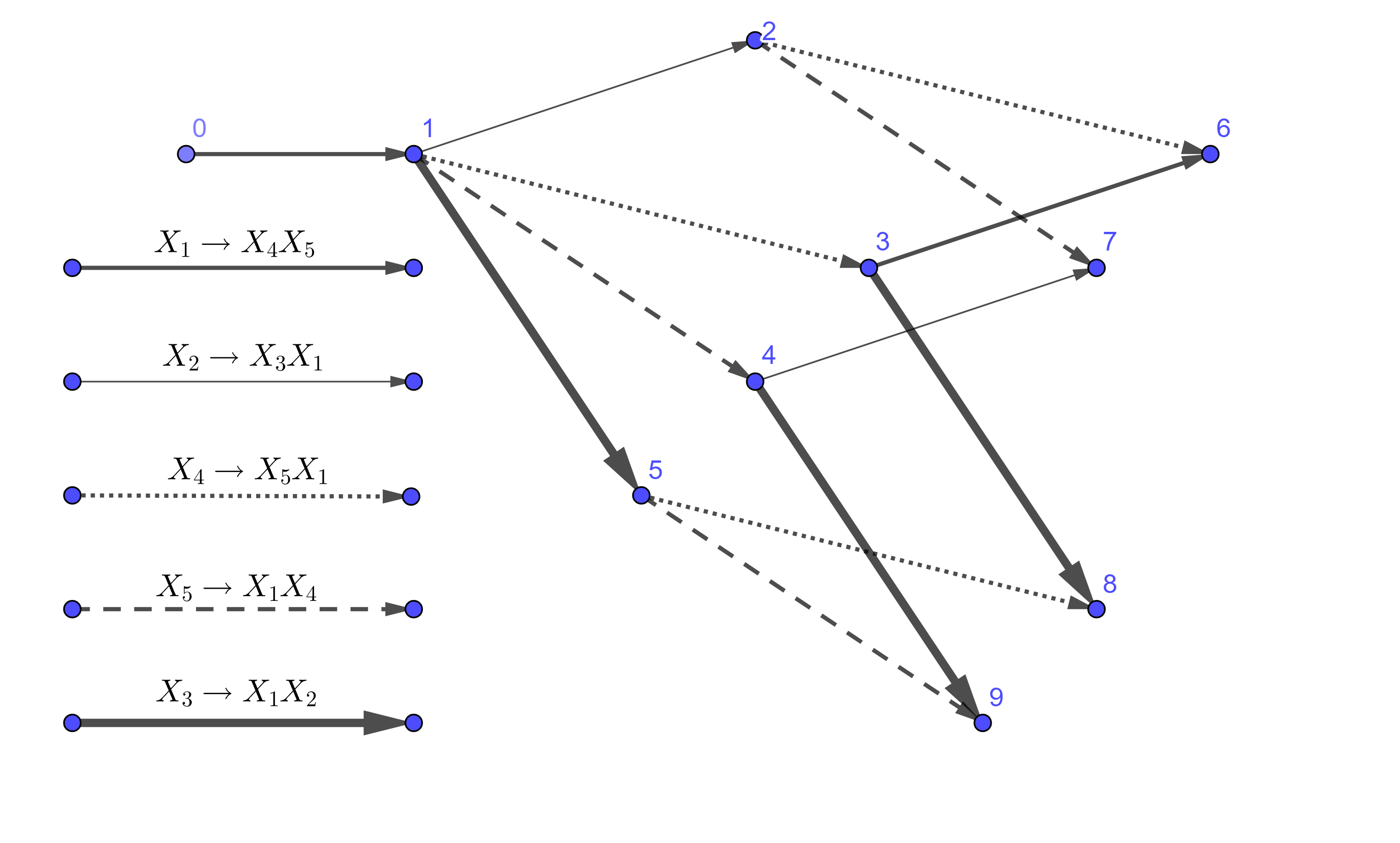
Figure 2: Even Length Palindrome Language

For the next example, let us consider the language generated by the grammar in table 1: a fragment of English that contains sentential recursion , as well as adjectival recursion under an NP constituent.

,

S $\rightarrow$ NP VP	VP $\rightarrow$ V3 S
NP $\rightarrow$ D N | PN	PP $\rightarrow$ P NP
VP $\rightarrow$ V0	NP -> D $\bar{N}$
VP $\rightarrow$ V1 NP	$\bar{N}$ $\rightarrow$ A $\bar{N}$
VP $\rightarrow$ V2 PP	$\bar{N}$ $\rightarrow$ A N

Table 1: A fragment of English

The shortest (POS-tagged) sentence of the language is PN V₀, for which the only maximally fitting grammar is $\{$ S $\rightarrow$ X₁, X₁ $\rightarrow$ X₂ X₃ $\}$ [X${}_{2}\rightarrow$ PN, X${}_{3}\rightarrow$ V₀] (point 0 in figure 3).

The next two shortest sentences are D N V₀ and PN V₁ PN. Adding the rules $\{$ X${}_{2}\rightarrow$ X₄ X₅} [X${}_{4}\rightarrow$ D, X${}_{5}\rightarrow$ N] or $\{$ X${}_{3}\rightarrow$ X₆ X₂ $\}$ [X${}_{6}\rightarrow$ V₁] result in maximally fitting grammars for these sentences, respectively (points 1 and 2 in figure 3). These two rules are unordered with respect to each other.

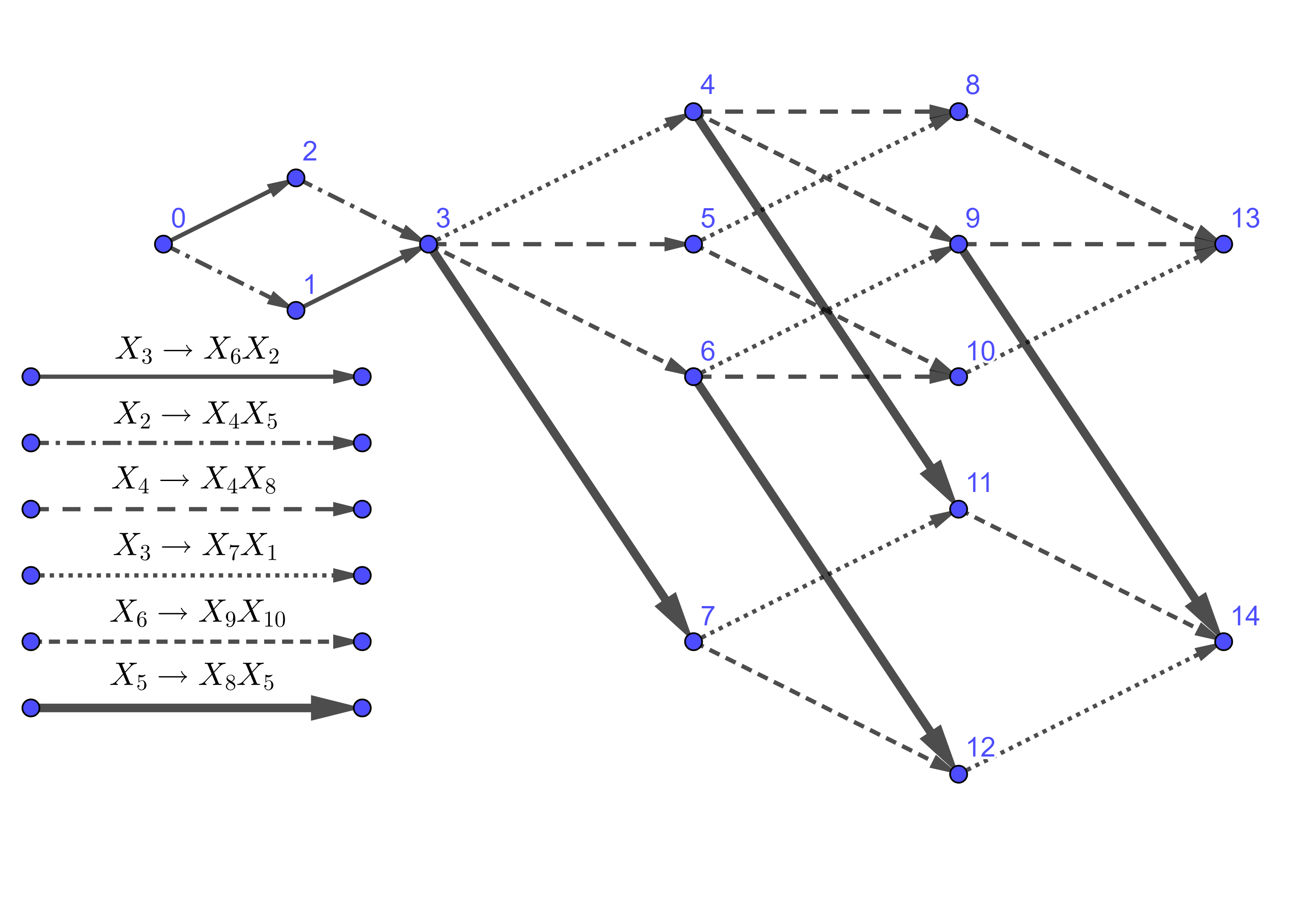
Figure 3: Left/Right recursion of Adjectives under an NP constituent

Having maximally fitted the simpler parts of the language, other two unordered rules must be learned now: (i) $\{$ X${}_{3}\rightarrow$ X₇ X₁} [X${}_{7}\rightarrow$ V₃] parses the sentence PN V₃ PN V₀ and (ii) $\{$ X${}_{6}\rightarrow$ X₉ X₁₀} [X${}_{9}\rightarrow$ P, X${}_{10}\rightarrow$ V₂] parses the sentence PN V₂ P PN.

Lastly, in order to maximally fit the recursion of the nonterminal A under NP constituents, two mirror-image rules are possible: (i) left recursion $\{$ X${}_{4}\rightarrow$ X₄ X₈} [X${}_{8}\rightarrow$ A], or (ii) right recursion $\{$ X${}_{5}\rightarrow$ X₈ X₅} [X${}_{8}\rightarrow$ A]. These two paths are mutually exclusive, but unordered with respect to the previous two rules. The result is 2 globally optimal grammars (points 13,14 in figure 3) which differ only with respect to the choice of right or left recursion. The grammar shape vector of the global optimal solution is given in table 2. In total, in order to successfully learn a grammar that is weakly equivalent to the target grammar, the learner requires 51 different basic (non-pumped) sentences.

depth	4	5	6	7	8
count	1	3	14	15	18

Table 2: Grammar Shape Vector

It is important to note that the learner was given the meta-parameter $k=1$, so only grammars in the 1-GROWTH CFG class are reached (i.e, the local optima are direct adjacents in the search space). Both these solutions show PP-Reanalysis in which the verb and the preposition are grouped together in a single constituent (e.g, X${}_{6}\rightarrow$ V₂ P). This is because a PP-Constituent requires both VP $\rightarrow$ V₂ PP and PP $\rightarrow$ P NP rules, and there is no local optimum that includes only one of them. The same holds true for ergative grammars: the rule SubectP $\rightarrow$ NP VP_erg requires also the presence of the rule VP_erg $\rightarrow$ $\Delta$; there is no local optimum that includes only one of those rules. Ergative grammars and PP-Consitutents therefore belong to the 2-GROWTH CFG class and are discoverable when the learner casts a wider net and is run with $k=2$. Due to a lack of space, please see the supplementary material for the set of global optima and their learning paths through the BFS for $k=2$ of the language above, as well as for the Odd-Length Palindrome language and languages with ambiguous grammars (for example, PP-Adjunction, VP $\rightarrow$ VP PP, NP $\rightarrow$ NP PP).

6 Learnability

Gold Gold (1967) in his seminal paper proved that if a class of languages $C$ contains all finite languages and at least one infinite recursive language, then it is not learnable (i.e, not identifiable in the limit). Amongst other limitations, Gold’s assumption that a learner should be able to identify a class in the limit given any presentation, including an adversial one, is too strong. I show below that once several conditions are met, learnability is achievable: (i) the unknown grammar that generated the target language is Context Free. (ii) the input is non-adversial (defined below), (iii) the fitness function incorporates indirect negative evidence, and (iv) the distance (the number of edges in the hypotheses space) between the optimal grammars does not exceed some constant $k$.

If the unknown grammar that generated the target language $\mathbb{L}$ is Context Free, then the learner knows that the infinite recursion of the target language develops in predictable manner. So, contra a fully-fledged recursively enumerable language (a Turing machine), it is not possible to select any arbitrary string in order to trick the learner. The set of misleading strings is constrained to the ones which might appear in CF languages. The learner also knows that the amount of basic (e.g, non-pumped) different strings that a grammar generates is finite (follows from the pumping lemma).

Let us define non-adversial presentation in the following way:

Definition 6.1 (Non-adversial text)

If there exists a finite time point $t_{j}$ after which every element from the set of all basic (non-pumped) strings $\mathbb{D}=\{s|s=u(v)w(x)y\}$ (of the unknown grammar $G$ which generated the target language $\mathbb{L}$) has been encountered in the presentation, then the presentation is non-adversial.

Lemma 6.1

Given a non-adversial presentation, $t_{j}$ (as defined above) is a mind-change bound.

Proof: Assume in contradiction that the teacher presents to the learner (from the true unknown optimal $G$) a string $s_{l}$ from $\mathbb{L}$ at $t_{l}>t_{j}$ which forced the learner into adding a new grammar to the set of possible candidates. By definition of non-adversial input, this string must be pumped. Hence, its basic counterparts, s=uwy and s=u(v)w(x)y appeared in the text up to $t_{j}$. Given the indirect negative evidence fitness function (repeated in 11, there is only a finite number of minimal globally optimal (i.e, maximally fitting) grammars that yield these basic strings, one of which generates $s_{l}$. The finiteness of the set of global optima stems from the fact that the length of a maximally fitting grammar $G$ is bound from above by the length of the ad-hoc grammar which has the longest description out of all maximally fitting grammars (Solomonoff (1964)). Thus at $t_{j}$ the learner predicted the possibility of $s_{l}$ given at time $t_{l}$, in contradiction.

$$f(D|G)=\sum_{i=1}^{max_{k}}\frac{ES(D,G)_{i}}{GS(G)_{i}}$$ (11)

Theorem 6.2 (Learnability of classes of CFL)

Let $C$ be a class of CFL such that for every $L\in C$ there is some grammar $G$ that generates it, L(G), $G\in k$-GROWTH class (or lower). Under the condition of non-adversial input, $C$ is identifiable in the limit with a learner with meta-parameter $k$ (which expresses the maximum distance between nearest local optima).

As shown, the BFS traversal leaves us only with a finite number of optimal grammars that maximally fit the basic strings $\mathbb{G}=\{G_{1},G_{2},\dots G_{n}\}$ and parse the rest of the input, $D$. Each $G_{i}$ yields $D$, but parses it differently. The learner can predict the ways in which each grammar generates recursive strings, and further evidence (which may appear before or after $t_{j}$) with pumped strings allows the learner to eliminate incorrect grammars from $\mathbb{G}$. Without further evidence to the contrary, they are all weakly equivalent candidates to the unknown grammar that generated the input $D$ seen so far. If the presentation is complete, i.e, all strings appear at least once, convergence to a weakly equivalent target grammar is guaranteed.

In Gold’s terms, the class above is identifiable in the limit, because a learner will produce a finite number of wrong grammars (up to some $t_{j}$), and remain with a set of candidate grammars, which the learner need not announce. The teacher might present further evidence arbitrarily long afterwards, which can be used to eliminate a finite number of wrong candidates. Crucially, a learner provided with meta-parameter $k$ is able to reach global optima (with a BFS) because there is a path leading to them in the search space, with optimal solutions which are not space more than $k$ edges apart.

There are two problems remaining. First, how does the learner identify the crucial time point $t_{j}$? That is, the moment in which the learner heard all basic strings $\mathbb{D}=\{s|s=u(v)w(x)y\}$, given some arbitrary probability distribution over $\mathbb{L}$. The problem is reduced to the missing probability mass problem. What is the probability of yet unobserved basic strings? This well-studied problem is prevalent in almost any application that samples from a discrete set. It is beyond the scope of this paper to discuss parametric and distribution-free methods of estimating the missing mass, the most famous of which is the Good-Turing estimator $n_{1}/N$, where $n_{1}$ is the number of the samples that appear once, and $N$ is the sample size (see Ben-Hamou et al. (2017), Good (1953), McAllester and Ortiz (2003) to name a few). Suffice it to say that if the presentation is non-adversial, the time-point $t_{j}$ is reached with probability 1, and the learner must estimate whether it has yet been reached. In practise, if the strings in the language grow fast enough, it is unlikely to encounter every single basic string. The learner must allow some degree of unseen mass and modify confidence accordingly. This can be done in parallel with more elaborate methods that estimate the unknown probability distribution over the target language. I leave such improvements for future research.

The second problem is that the learning algorithm assumes that the distance between nearest optimal solutions does not exceed some maximum $k$. That is, it is unknown whether the target language has a grammar that generates it in the $k$-GROWTH class (or lower). A possible heuristic is to have a variable $k$ that follows the rate of growth of sentences length in the input. Alternately, $k$ can be iteratively increased. I also leave improvements in discovery methods of $k$ for future research.

7 Complexity

Time complexity: the fitness function is computed at each point of the hypothesis space, i.e, the grammar and evidence shape vectors. For the evidence shape, the input $D$ is parsed according to some CFG parser (the implementation here uses an Early parser with $O(n^{3})$ where $n$ is the sentence length, see section 4. Dynamic programming computation (2.2) is employed to calculate the grammar shape. In practise, the time to parse the input outstrips the time required to compute the grammar shape vector, since the complexity of computing the grammar shape vector depends only on $G$ which is almost constant with respect to $D$.

Thus, at most $O(mn^{3})$ is spent to evaluate the fitness function $f(D|G)$ for some $G$ ($m$ is the number of sentences). Time complexity for a BFS is linear with the the visited vertices and edges in the powerset lattice of the hypotheses space.

The learner only visits the optimal grammars and their neighbours (up to maximum distance $k$). While the number of optimal solutions (vertices) is a constant of the grammar (see section 6), the number of neighbours for each vertex is bound from above by the number of production rules, which in itself, given CNF representation, is bound by $|V|^{3}$, where $V$ are the nonterminals ultimately appearing in the global solutions. Since the number of optimal grammars is constant, the time spent on traversing the search space is $O(c|V|^{3k})$ where $c$ is the number of optimal solutions.

In total, time complexity is $O(c|V|^{3k}mn^{3})$, where $V$ are nonterminals, $m$ number of sentences, $n$ maximum sentence length seen so far, $c$ number of optimal solutions, $k$ the maximum permitted distance between optimal grammars. Tighter upper bounds are possible but are left for future research. The number of optimal solutions, $c$, can be studied empirically. The learner is able to print the number of visited adjacents for each depth in the BFS graph, and compare it with the number of all grammars of the same length, which grows exponentially. Studying the sparsity of the the optimal points in the hypotheses space as a function of the grammar is beyond the current scope.

Space complexity At each point of the BFS, the adjacents list of the current grammar is requires (discarded when moving into the next frontier of the BFS) complexity $O(c|V|^{3k})$. In order to compute the fitness function, a temporary allocation $O(mn^{3})$ for the Earley parser is made but later discarded. Each optimal point only records the sentences indices in the input it successfully parsed. Total space complexity is bound from above by $O(c(m+|V|^{3k}))$; tighter bounds are possible.

8 Summary

In this paper, I explore whether incorporating a-priori knowledge about indirect negative evidence, which is a form of Bayesian inference, affects learnability of context free languages. The answer is positive, and new identifiable in the limit classes are found (see Angluin (1980), Clark and Eyraud (2007) for previous positive learnability results).

Under indirect negative evidence assumptions, absence of evidence is ultimately evidence for absence. If grammars are generative mathematical and/or mental objects, then we have access to the strings they generate, regardless of input. The fact that expected strings fail to appear in the text, after a sufficient number of samples, informs us that a candidate grammar underfits the data. The chosen fitness function $f$ introduced in section 2.3, repeated in 11) shows linearity with respect to the input and is motonoically nonincreasing with respect to the hypotheses space (a powerset lattice of production rules).

Thanks to optimal substructure (see section 3), an underfitting grammar and infinitely many grammars that contain its production rules $P$ as a subset can be eliminated from the enumeration of candidate grammars. Optimal substructure parallels convexity, in the sense that it allows us to discard an infinite part of the hypotheses space.

Global optima are reached with a greedy BFS through local optima and their adjacents. The learner is provided with a meta parameter $k$ which controls the maximum distance between nearest optima. This means that the learner is able to discover an optimal grammar belonging to $k$-GROWTH class.

The knowledge that a CFG generated the target language $\mathbb{L}$, means that despite the infinite presentation, the pumping lemma entails that the amount of structural information in a CFG is finite, and longer strings are fully predictable from shorter, basic strings, so the pumped strings contain no new information, given the grammar. A non-adversial text presentation supplies the learner with all these basic strings up to some time point $t_{j}$. This point is a mind-change bound, since there is only a finite number of maximally fitting grammars (according to the indirect negative evidence function $f$) that agree on these basic strings. The existence of a mind-change bound implies learnability since the learner can never be wrong.

Learnability here means that given a non-adversial input from an unknown target grammar $G$ that generates a target language $\mathbb{L}$, then if there is a weakly equivalent grammar $G\in k$-GROWTH that generates the same $\mathbb{L}$, a learner (with a meta-parameter $k$) is guaranteed to find it. Learners are able to identify in the limit classes of Context Free Languages (see 6.2) with varying degrees of time complexity. These novel positive learnability results demonstrate that it is possible to deterministically learn context free languages with very little input, and shed further light on the argument from the poverty of stimulus.

9 Appendices

Algorithm 1 The Learner

1:procedure BFS

2:     root $\leftarrow$ Node($\emptyset$)

3:     currentQueue.Enqueue(root)

4:     OptimalSolutions $\leftarrow$ $\emptyset$

5:     BannedSolutions $\leftarrow\emptyset$

6:     repeat

7:         for $i\leftarrow 0,currentQueue.Length$ do

8:              $G$ $\leftarrow$ currentQueue.Dequeue()

9:              $POSAssignments$ = MaxFitNextUnparsedSentence($D,OptimalSolutions$)

10:              BannedPOSAssignments $\leftarrow\emptyset$

11:              for $j\leftarrow 0,POSAssignments.Length$ do

12:                  $GS$ $\leftarrow$ ComputeGS($G$, POSAssignments[$j$])

13:                  $ES$ $\leftarrow$ ComputeES($G$, POSAssignments[$j$], $D$)

14:                  fitness $\leftarrow$ ComputeFitness(GS, ES)

15:                  if fitness=1 then

16:                       OptimalSolutions $\leftarrow$ OptimalSolutions$\cup\{$G $\}$

17:                  else

18:                       BannedPOSAssignments $\leftarrow$ BannedPOSAssignments $\cup\{$POSAssignments[$j$] $\}$                                 

19:              if $|G|$ < minSizeOfOptimalSolution OR currentNode.DistanceFromOptimal < $k$ then

20:                  attemptAdjacents = true               

21:              if attemptAdjacents = true then

22:                  adjacents $\leftarrow$ GetBFSAdjacents($G$, BannedPOSAssignments)

23:                  for each adjacent in adjacents do

24:                       visited[adjacent] = true

25:                       if bannedSolutions.ExistsSubset(adjacent) = false  then

26:                           nextQueue.Enqueue(adjacent)                                                                 

27:         currentQueue $\leftarrow$ nextQueue

28:         nextQueue $\leftarrow\emptyset$

29:     until currentQueue = $\emptyset$

References

- Angluin (1980) Dana Angluin. 1980. Inductive inference of formal languages from positive data. Information and control, 45(2):117–135.
- Bar-Hillel et al. (1961) Yehoshua Bar-Hillel, Micha Perles, and Eli Shamir. 1961. On formai properties oî simple phreise structure grammars. STUF-Language Typology and Universals, 14(1-4):143–172.
- Ben-Hamou et al. (2017) Anna Ben-Hamou, Stéphane Boucheron, and Mesrob I. Ohannessian. 2017. Concentration inequalities in the infinite urn scheme for occupancy counts and the missing mass, with applications. Bernoulli, 23(1):249 – 287.
- Chomsky (1981) Noam Chomsky. 1981. Lectures on government and binding, foris, dordrecht. ChomskyLectures on Government and Binding1981.
- Clark and Eyraud (2007) Alexander Clark and Rémi Eyraud. 2007. Polynomial identification in the limit of substitutable context-free languages. Journal of Machine Learning Research, 8(8).
- Clark and Lappin (2010) Alexander Clark and Shalom Lappin. 2010. Linguistic Nativism and the Poverty of the Stimulus. John Wiley & Sons.
- Earley (1970) Jay Earley. 1970. An efficient context-free parsing algorithm. Communications of the ACM, 13(2):94–102.
- Gold (1967) E Mark Gold. 1967. Language identification in the limit. Information and control, 10(5):447–474.
- Good (1953) Irving J Good. 1953. The population frequencies of species and the estimation of population parameters. Biometrika, 40(3-4):237–264.
- Joshi (1987) Aravind K Joshi. 1987. An introduction to tree adjoining grammars. Mathematics of language, 1:87–115.
- Keller and Lutz (1997) Bill Keller and Rudi Lutz. 1997. Evolving stochastic context-free grammars from examples using a minimum description length principle. In Workshop on Automatic Induction, Grammatical Inference and Language Acquisition.
- Koza (1994) John R Koza. 1994. Genetic programming as a means for programming computers by natural selection. Statistics and computing, 4:87–112.
- McAllester and Ortiz (2003) David McAllester and Luis Ortiz. 2003. Concentration inequalities for the missing mass and for histogram rule error. Journal of Machine Learning Research, 4(Oct):895–911.
- Scott (2008) Elizabeth Scott. 2008. Sppf-style parsing from earley recognisers. Electronic Notes in Theoretical Computer Science, 203(2):53–67.
- Shieber (1985) Stuart M Shieber. 1985. Evidence against the context-freeness of natural language. In The Formal complexity of natural language, pages 320–334. Springer.
- Solomonoff (1964) Ray J Solomonoff. 1964. A formal theory of inductive inference. part i. Information and control, 7(1):1–22.
- Stolcke (1995) Andreas Stolcke. 1995. An efficient probabilistic context-free parsing algorithm that computes prefix probabilities. Computational Linguistics, 21(2):165–201.
- Tomita (2013) Masaru Tomita. 2013. Efficient parsing for natural language: a fast algorithm for practical systems, volume 8. Springer Science & Business Media.
- Wyard (1994) Peter Wyard. 1994. Representational issues for context free grammar induction using genetic algorithms. In Grammatical Inference and Applications: Second International Colloquium, ICGI-94 Alicante, Spain, September 21–23, 1994 Proceedings 2, pages 222–235. Springer.