10 kT axial magnetic field generated using multiple conventional laser beams

Abstract

Strong laser-generated magnetic fields have important applications in high energy density science and laboratory astrophysics. Although the inverse Faraday effect provides a mechanism for generating strong magnetic fields by absorbing angular momentum from a high-intensity laser pulse, it is not applicable to conventional linearly polarized (LP) Gaussian laser beams. We have dmeveloped a spatial arrangement that overcomes this difficulty by using multiple laser beams arranged to have a twist in the pointing direction. Using three-dimensional kinetic particle-in-cell simulations, we show that this arrangement is the key to generating a strong magnetic field. The resulting multi-kT picosecond axial magnetic field occupies tens of thousands of cubic microns of space and can be realized under a wide range of laser parameters and plasma conditions. Our scheme is well suited for implementation at PW-class laser facilities with multiple conventional LP laser beams.

1 Introduction

Strong magnetic fields are essential for research in high-energy-density (HED) science, astrophysics, and controllable nuclear fusion sciences. Plasma properties can be influenced by the presence of magnetic fields of different scales. For instance, astrophysical plasmas with a temperature and density of $10<T<100\ \rm{eV}$ and $10^{17}<n<10^{19}\ \rm{cm}^{-3}$ [1, 2, 3, 4, 5], respectively, can be magnetized with a magnetic field strength of about 10 T. Relativistic magnetic reconnection can be observed in such plasmas when the magnetic field strength reaches 1 kT [6, 7, 8, 9], since the Alfven velocity becomes comparable to the speed of light. In contrast to that, the HED plasmas found in the cores of stars and planets, and in the fuel of inertial confinement fusion, have much higher temperatures and densities, exceeding $1\ {\rm{keV}}$ and $10^{21}\ {\rm{cm}}^{-3}$, respectively. For these plasmas, a magnetic field strength of around 100 T can benefit electron transport when the cyclotron frequency is equivalent to or bigger than the collisional frequency. Additionally, a magnetic field strength of about 1 kT can be used to control relativistic electron beams, improving high-energy ion acceleration [10]. When the magnetic field strength exceeds 10 kT, the laser can propagate in the magnetized plasma with electron density above the critical density as a whistler mode [11, 12, 13, 14]. The extremely small electron Larmor radius in magnetic fields above 10 kT leads to characteristic quantum-mechanical phenomena such as the nonlinear Zeeman effect, Paschen–Back effect, and Harper Broadening effect [15, 16]. The energy density of a magnetic field is given by $\varepsilon_{B}=B^{2}/(2\mu_{0})$, which can be expressed as $\varepsilon_{B}~{}[{\rm{J\cdot m}}^{-3}]\approx 4\times 10^{11}B^{2}~{}[\rm{kT}]$. When the magnetic field strength exceeds 1 kT, we can study the properties and dynamics of matter under extreme conditions where the magnetic field energy density is greater than $10^{11}~{}\rm{J\cdot m}^{-3}$. This may bring new opportunities to the HED science which is usually defined by energy density exceeding $10^{11}~{}\rm{J\cdot m}^{-3}$. The generation of strong magnetic fields in plasmas is of great interest due to its potential for a wide range of applications [17], including magnetically enhanced fast-ignition fusion [18], generation of collisionless shocks in magnetized plasmas [19, 20], magnetically assisted ion acceleration [21, 22, 23, 24, 25, 26], and magnetic field reconnection research [27]. In order to investigate the impact of strong magnetic fields, various approaches have been proposed and developed to generate fields over 100 T in laboratory environment. These include the use of pulsed-power devices [28, 29, 30], self-generated magnetic fields [31, 32, 33, 34, 35], magnetic flux compression [36, 37, 38, 39], and laser-driven coils [40, 41]. The corresponding measurement techniques of the magnetic field have also made significant strides in development [42, 43]. The magnetic flux compression technique has been a widely used method for generating high magnetic fields in laboratory experiments. One advantage of this technique is the use of non-destructive, single-turn coils driven by pulsed-power devices to generate magnetic fields of several tens of tesla for long durations ($>1~{}\rm{\upmu s}$) and large volumes ($>1~{}\rm{mm}^{3}$) [28, 29, 30]. By utilizing these magnetic fields as a seed field, a strong magnetic field over 100 T can be generated using the flux compression method. Alternatively, the scheme based on laser-driven coil can utilize high-power lasers with an intensity of approximately $10^{15}~{}{\mathrm{W}\cdot\mathrm{cm}^{-2}}$ to generate a magnetic field exceeding 100 T without requiring compression and a seed magnetic field. However, the underlying mechanism of how the laser-driven coil produces such a strong magnetic field is not fully understood, and its effectiveness remains a topic of debate. In a recent study, Peebles et al. [44] conducted extensive experiments to assess the potential of laser-driven coils in generating strong magnetic fields. The authors used different types of laser-driven coils to generate magnetic fields and employed various diagnostic techniques such as B-dot probing, Faraday rotation, and proton radiography [45] to measure the fields. Their conclusion is that the laser-driven coils cannot create quasi-static kilotesla-level fields as claimed [44].

At the same time, high-intensity laser systems have become increasingly important in strong magnetic field generation by inducing strong electric currents. With the invention of the Chirped Pulse Amplification (CPA) [46] technique, laser pulses are amplified to possess an ultra-high energy density. A laser pulse with high-intensity is an excellent driver for strong electrical currents suitable for generation of extremely strong magnetic fields. During the interaction between a high-intensity laser and an overdense plasma, the self-generated magnetic field on the plasma surface can be close in strength to the oscillating laser magnetic field [47]. Though such high amplitude magnetic fields are not in the bulk and have a complex topology, they can have an effect on generation of hot electrons [48].

Generation of strong magnetic fields in a large volume requires the use of laser beams with both high-intensity and high energy. Assuming the energy conversion from the laser into magnetic fields is 0.5%, a laser energy as high as 80 J is required to generate a 1 kT field with a volume of $(100~{}{\upmu\mathrm{m}})^{3}$. If the volume of the laser beam at focus is the same as the volume of the magnetic fields and the energy conversion is around 1%, we can expect that the strength of the generated magnetic field is going to be around $B\approx 0.1B_{L}$ [49], where $B_{L}$ is the peak amplitude of the laser magnetic field. There has been a significant increase in the number of laser facilities around the world that are capable of producing peak power at the petawatt (PW) level [50]. Meanwhile, the beam energy of several systems can be in the multi-kJ range. Such multi-kJ PW-class laser systems as LFEX [51], NIF ARC [52], and Petal [53], composed of multiple linearly polarized (LP) beamlets, allow experimental investigation of magnetic field generation in bulk plasma within relativistic regime by delivering the highest energy within picoseconds. The multi-beamlet configuration is not only an essential feature of the laser system design, but also the key to advanced laser-plasma interaction regimes [54]. The SG-ii@ UP facility [55], which includes a picosecond (ps) petawatt laser and tens of kilojoules (kJ) nanosecond (ns) lasers, is now being upgraded to a larger scale laser physics platform with multiple kJ-class ps laser beams and hundreds of kJ ns lasers. With the increased number of laser beams, the upcoming extended platform will provide the multi-beamlet experimental capacity of kJ-class ps petawatt lasers.

One particular mechanism for producing self-generated magnetic fields is through the inverse Faraday effect (IFE), where an axial magnetic field is spontaneously generated when the laser transfers angular momentum (AM) to plasma electrons. There exist various methods for generating axial magnetic fields through AM transfer. In the early days, the IFE was mostly observed when circularly polarized (CP) radiation propagated through an unmagnetized plasma, resulting in the generation of a quasistatic axial magnetic field [56], yet the effect is not exclusive to a CP beam carrying spin angular momentum (SAM) but also applicable to a vortex beam carrying orbital angular momentum (OAM). It is now well-known that helical wavefronts can be represented in a basis set of orthogonal Laguerre-Gaussian (LG) modes and that each LG mode is associated with a well-defined state of photon OAM [57]. The magnetic field generation using LG beams has been investigated theoretically and numerically [58, 59, 60].

While the IFE is widely studied, the optical technology and elements required for producing CP or LG laser beams from conventional LP beams at high power can be costly, complex, and fragile. As of now, the generation of adequately strong and precisely controllable macroscopic fields at laser facilities employed in HED physics research [50, 61, 55] remains a significant challenge. Recently, we have proposed a novel multi-beam approach for AM transfer to a plasma, leading to subsequent strong magnetic field generation [62]. The approach involves a spatial arrangement of four conventional laser beams, depicted in Fig. 1, that is inspired by the multi-beam design of the PW-class kJ laser systems. The key aspect of our design is its ability to overcome the challenge faced by conventional LP Gaussian lasers, which is that they do not possess intrinsic AM and thus cannot achieve the IFE. By employing the specific spatial arrangement of laser beams, we enable the transfer of ensemble AM to the plasma, inducing strong rotating currents, that lead to efficient generation of a strong axial magnetic field. This new multi-beam approach shows promising potential for enhancing magnetic field generation in laser-driven plasma systems.

Extending our previous work [62], in this paper we provide an in-depth analysis of the multi-beam approach. The wavelength of the driving laser beams is set to $1.053~{}{\upmu\mathrm{m}}$, which is the wavelength of the PW-class kJ laser beams at facilities like SG-ii@ UP. We examine the role of laser parameters (beam delay, polarization direction, phase offset) and target geometry (target with a preplasma vs. target with nanowires). We also compare our scheme with other schemes that employ CP or LG beams. The rest of this paper is organized as follows. Section 2 examines the AM carried by several conventional laser beams. In Section 3, we present the results of a 3D PIC simulation for four laser beams with twisted pointing directions. Section 4 is concerned with exploring the impact of laser parameters and target geometry on axial magnetic field generation. We compare different AM driving magnetic field generation schemes in Section 5. In Section 6, we summarize the main results of this work.

2 Angular momentum carried by laser beams

It is well known that paraxial optical beams carry three distinct types of AM [63]. They are SAM for CP beam, intrinsic OAM (IOAM) for LG beams with helical wavefronts and extrinsic OAM (EOAM) for normal beams propagating at a distance from the coordinate origin. The SAM is determined by the right- or left-hand CP. The IOAM is determined by the twist index of the LG beams. Both the SAM of a CP beam and the IOAM of a LG beam can be used for axial magnetic field generation via IFE [56, 58, 59, 60]. For EOAM, we can understand it from the viewpoint of photons carrying linear momentum $\bm{p}$ at position $\bm{r}$. The EOAM can be calculated as ${\bm{L}}^{\rm ext}=\bm{r\times p}$.

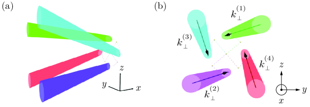
Figure 1: (a) 3D schematic of four beams with twisted pointing directions carrying AM collectively. The colored columns indicate the beams and the corresponding dash lines show the way that the twist is induced by the beams. (b) Each arrow is the component of the wave-vector (in a corresponding colored beam) transverse to the global direction ($x$-axis) of propagation of the ensemble of beams.

In order to take advantage of EOAM like SAM or IOAM in the IFE, we have proposed a setup that involves four laser beams with twisted pointing directions [62] that is schematically shown in Fig. 1. Each laser beam is represented by a colored cylindrical cone, with its direction determined by a wave vector $\bm{k}_{i}$, where $i$ is the index numbering the beam. The photon momentum in the $i$-th beam is $\bm{p}_{i}=\hbar\bm{k}_{i}$. For simplicity, consider two beams, the green and purple ones, with $\bm{k}_{(1,2)}=(k_{x},k^{(1,2)}_{\perp},0)$, intersecting the $(y,z)$-plane at $z_{(1,2)}=\pm f_{0}$ and $y_{(1,2)}=0$, respectively, where $f_{0}$ is the beam offset. In this case, the axial AM of a given photon is given by $[\bm{r}\times\bm{p}]_{x}$, where $\bm{r}$ is the position vector and $\bm{p}$ is the photon momentum. As a result, the total AM of the two beams is approximately

$$L_{x}\approx-N\hbar\left(k_{\perp}^{(1)}-k_{\perp}^{(2)}\right)f_{0},$$ (1)

where $N$ is the number of photons in one beam. If the two beams have the same tilt, then $k^{(1)}_{\perp}=k^{(2)}_{\perp}$ and, as a result, $L_{x}\approx 0$. If the tilt of the second beam is opposite to that of the first, then $k^{(2)}_{\perp}=-k^{(1)}_{\perp}$. As a result, the total AM no longer vanishes and it is roughly given by $L_{x}\approx-2N\hbar k_{\perp}^{(1)}f_{0}$. The total AM will double when a pair of such lasers with an offset in the $y$ direction is added, showing that appropriately arranged beams can carry AM even though individual photons in each beam have no intrinsic AM [63]. This observation bears similarities to studies involving $\gamma$-ray beams carrying OAM [64, 65, 66], where a population of photons with a twisted distribution of momentum $\bm{p}$ is generated. An alternative method is to calculate the AM of electromagnetic field as

$$\bm{L}=\varepsilon_{0}\int\left(\bm{r}\times\left[\bm{E}\times\bm{B}\right]\right)d^{3}{r}.$$ (2)

where $\varepsilon_{0}$ is the dielectric permittivity and $\bm{E}$ and $\bm{B}$ are the electric and magnetic fields, respectively. Note that $[\bm{E}\times\bm{B}]$ matches the direction of the Poynting vector. In a given laser beam, the dominant component of the Poynting vector is directed along the axis of the beam. Therefore, four laser beams with a twist in the pointing direction (shown in Fig. 1) can possess net AM.

3 Simulation results for beams with twisted pointing directions

In this section, we present a self-consistent analysis performed using three-dimensional (3D) particle-in-cell (PIC) simulations with the open-source relativistic PIC code EPOCH [67]. As explained in Section 2, our goal is to take advantage of the multi-beam configuration available at some state-of-the-art PW-class laser systems. We consider a laser system that provides four identical LP Gaussian laser beams that have no intrinsic AM. The peak intensity of each laser beam is $I_{0}=8.0\times 10^{19}~{}{\mathrm{W}\cdot\mathrm{cm}^{-2}}$, which corresponds to a normalized electric field amplitude $a_{0}=8.0$. The normalization of the electric field is defined as $a_{0}=eE_{0}/m_{e}\omega c$, where $E_{0}$ is the peak electric field amplitude. Where $c$ is the speed of light, $\omega$ is the center frequency of the laser beam, and $e$ and $m_{e}$ are the electron charge and mass, respectively. The pulse duration, $\tau_{g}=600$ fs, is the same for each beam (the temporal envelope of the electric field is Gaussian). The laser wavelength is $\lambda=1.053~{}{\upmu\mathrm{m}}$ and the beam waist radius is $w_{0}=6.0~{}{\upmu\mathrm{m}}$.

Parameters of four laser beams
Peak intensity	$I_{0}=8.0\times 10^{19}~{}{\mathrm{W}\cdot\mathrm{cm}^{-2}}$
Normalized field amplitude	$a_{0}=8.0$
Wavelength	$\lambda=1.053~{}{\upmu\mathrm{m}}$
Focal spot size ($1/\mathrm{e}$ electric field)	$w_{0}=6.0~{}{\upmu\mathrm{m}}$
Pulse duration (Gaussian electric field)	$\tau_{g}=600$ fs
The global direction of propagation of the ensemble of beams	$+x$
Linear polarization in the emitter plane	$+y$
Location of the emitter plane	$x_{e}=-20.0~{}{\upmu\mathrm{m}}$
Location of the focal plane	$x_{f}=-5.0~{}{\upmu\mathrm{m}}$
Beam offset in the focal plane	$f_{0}=11.0~{}{\upmu\mathrm{m}}$
The polar and azimuth angle for convergence and twist	$\theta=0.27\pi$, $\varphi=0.28\pi$
Other parameters
Foil thickness	$x\in[0,3]~{}{\upmu\mathrm{m}}$
Preplasma thickness	$x\in[-5,0]~{}{\upmu\mathrm{m}}$
Modulation mode of preplasma	$+x$ exponential
Electron density	$n_{e}=50.0\;n_{c}$
Ion (C6+) density	$n_{i}=50.0/6\;n_{c}$
Simulation box	$(40~{}{\upmu\mathrm{m}})^{3}$
Spatial resolution	25 cells/${\upmu\mathrm{m}}$
Macroparticles per cell	4
Location of the front surface of the foil	$x=0~{}{\upmu\mathrm{m}}$
Time when the laser beams leave the simulation box	$t=0$ fs

Table 1: 3D PIC simulation parameters. $n_{c}=1.0\times 10^{21}$ cm^-3 is the critical density for the considered laser wavelength. The initial temperature is set to zero. The electron to ion mass ratio is $1/(1836\times 12)$.

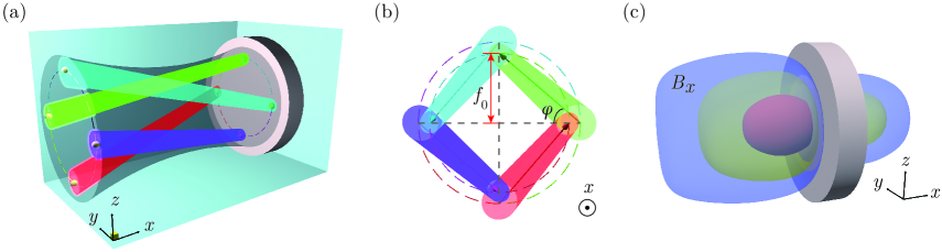
Figure 2: (a) 3D schematic of the target and four regular laser beams with twisted pointing directions represented by colored conical cylinders. (b) 2D projection of the beams onto the $(y,z)$-plane, showing the beginning and the end in the emitter plane and the focal plane, respectively. The parameters can be found in Table 1. (c) Illustration of the axial magnetic field $B_{x}$ after the lasers have left the simulation box ($t=20$ fs). The blue, yellow, and red isosurfaces, from the outside to the inside, represent increasing magnetic field strength. The axial magnetic field profile is quantified in Fig. 3.

The orientation of the four laser beams is set according to Fig. 2 (a), where the lasers are represented by colored conical cylinders. For each beam, the axis represents the propagation direction and the transverse size represents the beam radius. The lasers enter the simulation domain from the left boundary of the simulation box ($x_{e}=-20~{}{\upmu\mathrm{m}}$) that we refer to as the emitter plane. They interact with the plasma at the focal plane located at $x_{f}=-5~{}{\upmu\mathrm{m}}$. The transverse electric field of each beam in the $(y,z)$-plane is set to be directed along the $y$-axis. Figure 2 (b) shows projections of all four beams onto the $(y,z)$-plane. The beams are set up such that the intersection points of the beam axes with the $(y,z)$-plane for a given longitudinal position $x$ form vertices of a square. This square formed by the intersection points rotates and shrinks as the beams propagate from the emitter plane to the target. To make it more evident that the intersection points get closer to each other as the beams approach the target, we also plotted two circles that go through the intersection points in the emitter plane and the focal plane. The circle in the focal plane is visibly smaller. The radius of the circle in the focal plane is $f_{0}$. We call it the beam offset. The twist degree of four laser beams is controlled by the azimuthal angle $\varphi=0.28\pi$. By definition, there is no twist for $\varphi=0$. The angle between the axis of every beam and the focal plane (in the plane formed by the beam axis and the $x$-axis) is $\theta=\arctan(S/D)=0.27\pi$, which is the polar angle characterizing the beam convergence, where $D$ is the distance between the emitter plane and the focal plane and $S$ is the transverse shift of the beam axes in the two-dimensional projection plane.

We assume that the target is a fully ionized carbon plasma with an exponential longitudinal density profile to mimic a preplasma. The initial electron density is set to $n(x)=0.05n_{e}{\rm{exp}}\{(x~{}[{\upmu\mathrm{m}}]+5)/1.67\}$, where $n_{e}=50\;n_{c}$ is the electron density of the foil whose thickness is $3~{}{\upmu\mathrm{m}}$ behind the preplasma and $n_{c}=1.0\times 10^{21}$ cm^-3 is the critical density corresponding to a laser wavelength $\lambda=1.053~{}{\upmu\mathrm{m}}$. Both electron and ion populations are initially cold ($T$ = 0). The front surface of the foil is at $x=0$ and the rear surface is at $x=3~{}{\upmu\mathrm{m}}$. Using this profile, the plasma density ramps up from $3\;n_{c}$ to $50\;n_{c}$ over $5~{}{\upmu\mathrm{m}}$, which increases the interaction volume between the laser beams and the plasma. The simulation box size is $(40~{}{\upmu\mathrm{m}})^{3}$ with grid cell sizes of $(40~{}\rm nm)^{3}$. We use four particles per cell and have open boundaries throughout. Table 1 gives detailed parameters of the 3D PIC simulation presented here. It must be pointed out that our setup differs from that used in Ref. [62], where we employed nanowires rather than a preplasma and the laser wavelength was set to $0.8~{}{\upmu\mathrm{m}}$. We define the moment when the laser beams leave the simulation domain following their reflection off the target as $t=0$ fs. In the described simulation, we observe generation and gradual evolution of an axial magnetic field. The illustration of the axial magnetic field $B_{x}$ after the lasers have left the simulation box ($t=20$ fs) is shown in Fig. 2 (c). The blue, yellow, and red isosurfaces, from the outside to the inside, represent increasing magnetic field strength.

3.1 Magnetic field distribution

We observe generation of a strong axial magnetic field in the simulation when using beams with twisted pointing directions. Figure 3 (a) displays the axial magnetic field for $\varphi=0.28\pi$ at $t=20$ fs. The strength of the peak longitudinal magnetic field exceeds 10 kT. The volume occupied by the field stronger than 2 kT is approximately $10^{4}~{}{\upmu\mathrm{m}}^{3}$. The three volumetric isocontours indicate $B_{x}/B_{0}=-0.2$, $-0.55$, and $-0.8$, where $B_{0}=2\pi m_{e}c/|e|\lambda=10.0~{}\rm kT$. To provide a clearer $B_{x}$ profile, the values are temporally averaged over a 20 fs interval and spatially smoothed using a box with a stencil size of $(0.4~{}{\upmu\mathrm{m}})^{3}$. Due to the approximately axisymmetric distribution of the magnetic field, for simplicity, we perform azimuthal averaging that yields the magnetic field strength distribution in the $(x,r)$-plane that is shown in Fig. 3 (b). The magnetic field reaches its peak strength of $1.4~{}B_{0}$ on axis at $x=-10~{}{\upmu\mathrm{m}}$. In addition, there is a clear presence of axial magnetic fields both in front and behind the target. The magnetic field strength and its variation gradient are generally larger in front of the target. It is worth mentioning that although the magnetic field strength behind the target is weaker than the magnetic field in the front, its strength can still reach thousands of Tesla. This confirms that our scheme does indeed produce OAM-bearing electrons, since the lasers are unable to reach behind the target. The presence of significant magnetic fields even in the region behind the target demonstrates the efficiency of the AM transfer mechanism and its ability to induce axial magnetic fields over a considerable distance.

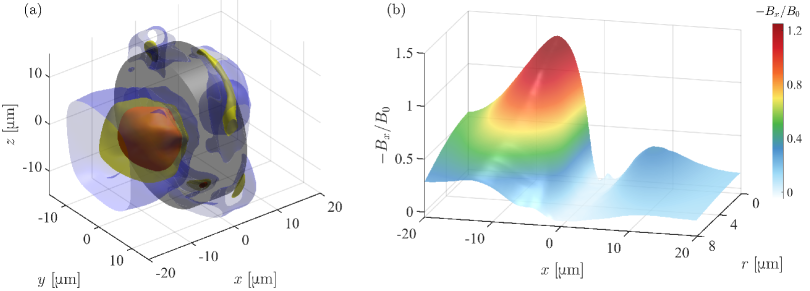
Figure 3: Distribution of the axial magnetic field at $t=20$ fs. (a) Volumetric isocontours of axial magnetic field component for $B_{x}=-0.2$, $-0.55$, $-0.8~{}B_{0}$ (purple, yellow, red). (b) Distribution of the axial magnetic field in the $(x,r)$-plane. Azimuthal averaging is performed.

To study the temporal evolution of the axial magnetic field, we perform longitudinal and azimuthal averaging over a cylindrical region of length $L$: $\left<B_{x}\right>(r)=1/(2\pi L)\int_{0}^{2\pi}\int_{0}^{L}B_{x}(r,\phi,x)dxd\phi$. We choose $L=5~{}{\upmu\mathrm{m}}$ according to the simulation result and show the distribution of $\left<B_{x}\right>(r,t)$ in Fig. 4 (a). We can see in Fig. 4 (b) that the magnetic field between $t=-600$ fs and $t=-500$ fs has the maximum growth rate $\Gamma_{in}=4.75\times 10^{-3}\omega$, where $\omega$ is the laser frequency corresponding to the laser wavelength $\lambda=1.053~{}{\upmu\mathrm{m}}$. As the hot electrons expand, the axial magnetic fields decay. We find that the characteristic decay rate is $\Gamma_{de}=-2.4\times 10^{-3}\omega$. The duration of the axial magnetic field is around $\tau_{B}\approx 1$ ps, which is in the same order of magnitude as the magnetic field generated by the IFE [60].

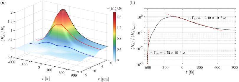
Figure 4: Temporal evolution of the axial magnetic field. (a) The distribution of the axial magnetic field in the $(t,r)$-plane, with slices highlighted at radial distance $r=0~{}\rm{(black)}$, $4~{}\rm{(red)}$, $8~{}\rm{(blue)}~{}{\upmu\mathrm{m}}$. Longitudinal and azimuthal averaging is performed. (b) Axial magnetic field for $r=0~{}{\upmu\mathrm{m}}$, where $\max\left\langle B_{x}\right\rangle=1.78~{}B_{0}$. $t=0~{}\rm fs$ is defined as the moment when the lasers leave the simulation space completely.

Figure 5 shows the axial magnetic field distribution at three different times: panels (a) - (c) correspond to $t=20.0$ fs, panels (d) - (f) correspond to $t=220.0$ fs, and panels (g) - (i) correspond to $t=420.0~{}\rm fs$. Figure 5 (a), (d), and (g) give the electron density normalized to the critical electron density $n_{c}$. The black contours denote $n_{e}=n_{c}$. The simulation confirms that the laser beams are reflected rather than being transmitted through the foil. Panels (b), (e), and (h) in Fig. 5 are transverse slices of the axial magnetic field (averaged over 20 fs output dumps and normalized to $B_{0}=2\pi m_{e}c/|e|\lambda=10.0~{}\rm kT$). The two black solid lines represent the front ($x=0~{}{\upmu\mathrm{m}}$) and the back ($x=3~{}{\upmu\mathrm{m}}$) of the foil, respectively. The front ($x=-5~{}{\upmu\mathrm{m}}$) of the exponentially modulated preplasma is represented by the black dashed lines. We find that the magnetic field region moves axially outward. Panels (c), (f), and (i) in Fig. 5 show radial lineouts of the axial magnetic field averaged azimuthally, temporally (over 20 fs), and longitudinally between the red and black dashed lines in Fig. 5 (b), (e), and (h). The results show that the magnetic field expands radially outwards, which leads to the reduction of its peak strength.

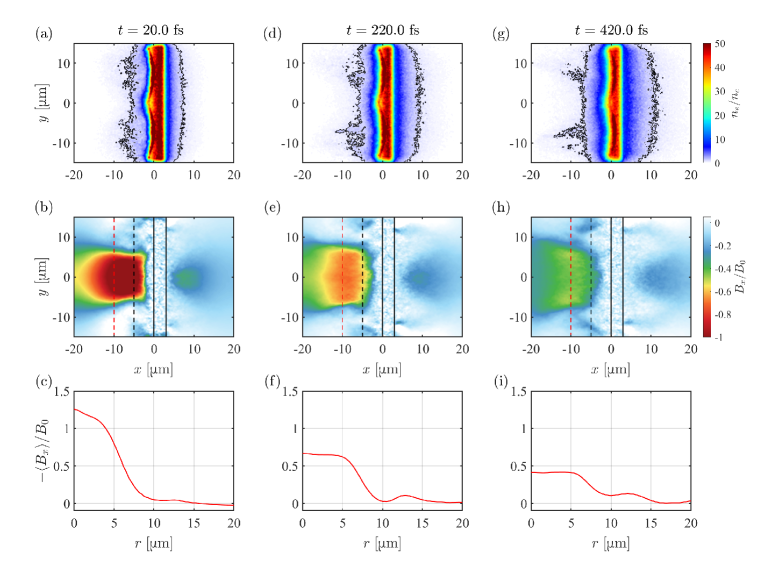
Figure 5: Simulation results at three different times, $t=20.0$, 220.0, and 420.0 fs (from left to right). (a), (d), and (g) Longitudinal slices of electron density, where the density is normalized to the critical density and the black solid lines mark $n_{e}=n_{c}$. (b), (e), and (h) Longitudinal slices of the axial magnetic field, where the field is averaged over 20 fs and normalized to $B_{0}=2\pi m_{e}c/|e|\lambda=10.0~{}\rm kT$; the two black solid lines respectively represent the front ($x=0~{}{\upmu\mathrm{m}}$) and rear ($x=3~{}{\upmu\mathrm{m}}$) surfaces of the solid part of the target; the front surfaces ($x=-5~{}{\upmu\mathrm{m}}$) of exponentially modulated preplasma are represented by the black dashed lines; the red and black dashed lines show the boundaries of the lineout region. (c), (f), and (i) Radial lineouts of the axial magnetic field, where the field is averaged azimuthally, temporally, and longitudinally (over the lineout region marked with red and black dashed lines in the middle row). Laser-plasma parameters are given in Table 1.

Though our main focus is on the axial magnetic field, we provide longitudinal slices of all three components of the generated magnetic field at $t=20$ fs. In Fig. 6, $B_{x}$, $B_{y}$, and $B_{z}$ are shown in $(x,y)$-plane (top row) and $(x,z)$-plane (bottom row), respectively. These slices provide important reference values for the following discussion of the dependence of the magnetic field on the angle of twist. These results also confirm that the axial magnetic field is indeed very axisymmetric in our scheme. It is worth noting that in the region of peak axial magnetic field, the transverse components are generally an order of magnitude smaller in strength. Furthermore, these transverse fields reach their peak values away from the central core of the axial magnetic field. These transverse components are particularly weak near the axis. We can conclude that the magnetic field is axial only in the central region.

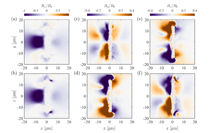
Figure 6: Two-dimensional longitudinal slices at $t=20$ fs of all three components of the time-averaged (averaged over 20 fs output dumps) magnetic field from the 3D PIC simulation with the parameters listed in Table 1. The fields are normalized to $B_{0}=2\pi m_{e}c/|e|\lambda=10.0~{}\rm kT$. $B_{x}$, $B_{y}$, and $B_{z}$ are shown in $(x,y)$-plane (top row) and $(x,z)$-plane (bottom row), respectively. Note that the color scale for $B_{x}$ is different from that for $B_{y}$ and $B_{z}$.

When considering the energy content in a box with $x\in(-15,-5)~{}{\upmu\mathrm{m}}$ and $y$, $z\in(-10,10)~{}{\upmu\mathrm{m}}$, we find that the energy in the magnetic field ($U_{B}=\int B_{x}^{2}/(2\mu_{0})dV\approx 1.6$ J) is much smaller than the total kinetic energy of electrons ($U_{e}\approx 20$ J). The total energy of the four incident lasers is $U_{\rm L}\approx 217$ J. We find that the energy conversion efficiency from laser to hot electrons and from hot electrons to the magnetic field are both around 10%. This overall conversion efficiency is similar to the conversion efficiency for the Biermann battery magnetic fields experimentally generated in laser-solid interactions (a maximum field strength of $B\approx 100~{}\rm T$ and lower bound of the magnetic energy 7.5 J driven by laser energy of 1 kJ) [68]. However, it is two orders of magnitude higher than the conversion efficiency for a laser-driven coil in Ref. [69]. This demonstrates the effectiveness of our multi-beam approach in efficiently converting laser energy into a strong magnetic field.

3.2 Azimuthal current distribution

We begin by analyzing the azimuthal current density $j_{\phi}$, which is believed to be responsible for the generation of the axial magnetic field. Figure 7 (a) illustrates the distribution of the azimuthal current density $j_{\phi}$ (averaged over the azimuthal angle) for $\varphi=0.28\pi$ at $t=20$ fs as a function of axial $x$ and radial $r$ positions. The current density is normalized to $j_{0}=-|e|cn_{c}=-4.8\times 10^{16}~{}\rm A\cdot m^{-2}$ which corresponds to the electrons with density $n_{e}=n_{c}=1.0\times 10^{21}$ cm^-3 rotating at the speed of light. The establishment of the strong azimuthal current $j_{\phi}$ shown in Fig. 7 (a) is crucial for the efficient generation of the strong axial magnetic field in our multi-beam approach. The negative azimuthal current should produce a negative axial magnetic field. This is the same direction as shown in Fig. 3 (a). Two-dimensional transverse slices of $j_{\phi}$ at $x=-10$ and $-5~{}{\upmu\mathrm{m}}$ are presented in Fig. 7 (b) and (c), respectively. As observed in Fig. 7 (a), the azimuthal current density $j_{\phi}$ at $x=-5~{}{\upmu\mathrm{m}}$ is stronger compared to the current density at $x=-10~{}{\upmu\mathrm{m}}$.

To estimate the maximum value of $|B_{x}|$, we make an order of magnitude assumption that $j_{\phi}$ is uniform within a cylindrical region of radius $R$ and length $2h$. After applying the Biot-Savart law [70], we obtain

$$\max|B_{x}| \approx \dfrac{\mu_{0}}{2}\int_{0}^{R}\int_{-h}^{h}|j_{\phi}|\dfrac{r^{2}}{(r^{2}+x^{2})^{3/2}}\mathrm{d}x\mathrm{d}r$$ (3)

$$= \mu_{0}|j_{\phi}|h\operatorname{arsinh}(R/h),$$

where $\mu_{0}=1.26\times 10^{-6}$ H/m is the permeability of free space. From the information provided in Fig. 7 (a), we can set $R\approx h\approx 5~{}{\upmu\mathrm{m}}$. Considering that the value of the azimuthal current density in Fig. 7 (c) is $|j_{\phi}|\approx 0.08~{}|j_{0}|$, where $j_{0}\equiv-|e|cn_{c}$, we can estimate the maximum value of $|B_{x}|$ as $\max|B_{x}|\simeq 20$ kT. This result is close to the peak magnetic field strength $\left<B_{x}\right>\simeq 1.8~{}B_{0}=18$ kT observed in Fig. 4 (b).

Assuming that the motion of the electrons is the main contributor to the current, we can calculate the effective azimuthal velocity as $v_{\phi}\approx-j_{\phi}/|e|n_{e}$. Furthermore, the azimuthal current density can be used to estimate the OAM density of hot electrons. With the electron density obtained from the simulations, $n_{e}\approx 10^{27}$ m^-3, we find that the rotation velocity is about $v_{\phi}\approx 0.1c$, which implies a fast rotating plasma environment. One may wonder if the rotating effect is just a combination of four cross currents forming a shape similar to a square. We can estimate the expanding effect of the cross currents (if these currents are indeed present) using $v_{\phi}\approx 0.1c$. After 400 fs (from $t=20$ fs to $t=420$ fs), the transverse shift should be $R_{S}=0.1c\times 400~{}{\rm fs}\approx 12~{}{\upmu\mathrm{m}}$. Such a significant shift is not observed in our simulation, which leads us to conclude that we are indeed dealing with a fast rotating plasma rather than with four cross currents. We can write the OAM density of electrons as $L_{xe}\approx r\gamma_{a}m_{e}n_{e}v_{\phi}$, where $\gamma_{a}$ is the relativistic gamma-factor and $n_{e}$ is the electron density. We next take into account that $j_{\phi}\approx|e|n_{e}v_{\phi}$ to obtain that $L_{xe}\approx r\gamma_{a}m_{e}j_{\phi}/|e|$. With $r=f_{0}$ and $\gamma_{a}\approx(1+a_{0}^{2})^{1/2}\approx 8$, the OAM density is approximately $L_{xe}\approx 2.4~{}{\mathrm{kg}\cdot\mathrm{m}^{-1}\cdot}\mathrm{s}^{-1}$. Compared to the case where twisted lasers are employed to generate OAM [71], our scheme produces a rotating plasma environment with electron density and rotation velocity that are two orders of magnitude higher.

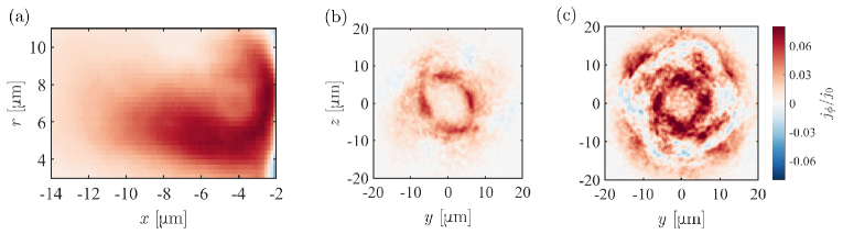
Figure 7: Azimuthal current density $j_{\phi}$ (normalized to $j_{0}=-|e|cn_{c}=-4.8\times 10^{16}~{}\rm A\cdot m^{-2}$) at $t=20$ fs. (a) Azimuthal current density $j_{\phi}$ averaged over $\phi$ as a function of $x$ and $r$. (b) and (c) Two-dimensional transverse slices of $j_{\phi}$ at $x=-10$ and $-5~{}{\upmu\mathrm{m}}$, respectively.

3.3 OAM distributions analysis

To study the rotational effect induced in the plasma and to quantify the AM transfer from the four laser beams with a twist angle of $\varphi=0.28\pi$ in our simulation, we analyze the density of axial OAM in electrons ($L_{xe}$) and ions ($L_{xi}$). Both quantities are normalized to a reference value $L_{0}\equiv n_{c}m_{e}cw_{0}\approx 1.65~{}{\mathrm{kg}\cdot\mathrm{m}^{-1}\cdot}\mathrm{s}^{-1}$, where $L_{0}$ represents electrons with density $n_{c}$ rotating with azimuthal velocity $v_{\phi}=c$ at a radial position with $r=w_{0}$. The analysis is conducted at a time of $t=20$ fs. In Fig. 8, the densities of axial OAM for electrons (top row) and ions (bottom row) are shown at $t=20$ fs. Figure 8 (a) and (b) show angle-averaged $L_{xe}$ and $L_{xi}$ as functions of $x$ and $r$. Further insight can be provided by two-dimensional transverse slices of $L_{xe}$ ($L_{xi}$) at two different axial locations, $x=-10~{}{\upmu\mathrm{m}}$ and $x=-5~{}{\upmu\mathrm{m}}$, shown in Fig. 8 (c) and Fig. 8 (e) (Fig. 8 (d) and Fig. 8 (f)), respectively. We would like to point out that the OAM density in Fig. C1 from the appendix of our previous work [62] is artificially high due to a data processing error.

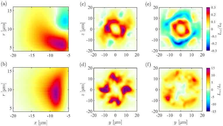
Figure 8: Density of axial OAM for electrons (top row) and ions (bottom row) normalized to $L_{0}\equiv n_{c}m_{e}cw_{0}\approx 1.65~{}{\mathrm{kg}\cdot\mathrm{m}^{-1}\cdot}\mathrm{s}^{-1}$ at $t=20$ fs in the simulation with the twist angle $\varphi=0.28\pi$. (a), (b) Azimuthally averaged densities of axial OAM $L_{xe}$ and $L_{xi}$ as functions of $x$ and $r$. (c), (d) and (e), (f) Transverse slices of $L_{xe}$ and $L_{xi}$ at $x=-10$ and $-5~{}{\upmu\mathrm{m}}$, respectively.

As can be seen from Fig. 8 (c) and (e), when comparing the results at $x=-10~{}{\upmu\mathrm{m}}$ with those at $x=-5~{}{\upmu\mathrm{m}}$, the axial OAM density of electrons at $x=-10~{}{\upmu\mathrm{m}}$ displays a higher OAM intensity and a broader distribution. In contrast, the axial OAM density distribution range of ions in the longitudinal direction is smaller than that of electrons. This behavior could stem from the challenges involved in altering the motion state of ions. While the axial OAM density of electrons remains positive and gradually decreases away from the target in most of the region ($x<-7.5~{}{\upmu\mathrm{m}}$), another intriguing phenomenon is the occurrence of negative axial OAM density for electrons near the preplasma ($x\in[-7.5,-5]~{}{\upmu\mathrm{m}}$), indicating a reversal of electron rotation at larger radial positions. Over time, the hot electrons undergo radial and longitudinal expansion away from the target, which is likely to contribute to the reduction in axial magnetic field strength. According to Fig. 8, we can approximate the distribution ratio of the OAM density between electrons and ions as $\eta_{ei}=L_{xe}/L_{xi}\approx 1\%$. We attribute this observation to the significant mass disparity between ions and electrons (where $m_{i}/m_{e}\approx 10^{4}$). Despite the higher OAM density of the ions, the velocity of the ions is still much less than that of the electrons. Since the current does not depend on particle masses, these simulation results confirm our earlier assumption that the dominant contribution to the azimuthal current component comes from electron motion.

To construct an analytical model for this new scheme, we begin by examining the AM density of the four laser pulses. This AM density, denoted as $L_{x}=\varepsilon_{0}(\bm{r}\times[\bm{E}\times\bm{B}])_{x}$, vanishes on the axis and reaches its maximum value at the beam offset. In light of the extensive simulation results we presented earlier, we now turn our attention to the process of AM absorption. We envision this absorption occurring within a cylindrical region of radius $R$ and length $2h$. The lasers, first and foremost, impart AM to electrons. Through the electron current, a strong axial magnetic field is generated. During the generation phase, the evolving magnetic field introduces an azimuthal electric field $E_{\phi}$. This electric field, in turn, facilitates the transfer of absorbed OAM from electrons to ions. The electrons and ions are assumed to rotate rigidly in a shell with angular velocities $\zeta_{e}$ and $\zeta_{i}$, respectively. Since the particles are moving away from the center, we expect it to work well only for estimating initial peak values. We introduce OAM to describe the rotational motion of electrons and ions, denoted as $L_{e}=I_{e}\zeta_{e}$ and $L_{i}=I_{i}\zeta_{i}$ respectively. Here, $I_{e}$ is the moment of inertia for electrons and is given by $I_{e}=\pi R^{4}hm_{e}n_{e}$. Meanwhile, $I_{i}$ represents the moment of inertia for ions and is calculated as $I_{i}=(m_{i}/Zm_{e})I_{e}$, where $Z$ is nuclear charge number of ions. These OAM estimates capture the rotational dynamics of the charged particles. The overall evolution of the OAM of electrons and ions can be described by the following equations [72]

$$I_{e}\frac{d\zeta_{e}}{dt}=M_{\rm abs}-M_{\rm E},~{}~{}I_{i}\frac{d\zeta_{i}}{dt}=M_{\rm E},$$ (4)

where $M_{\rm abs}$ represents the torque resulting from OAM absorption. The term $M_{\rm E}$ signifies the torque due to the azimuthal electric field $E_{\phi}$ and can be expressed as $M_{\rm E}=\int|e|E_{\phi}(r)rn_{e}d^{3}r\approx|e|E_{\phi}(R)I_{e}/(m_{e}R)$. The rotational motion of electrons generates current density $j_{\phi e}$, which can be approximated as $j_{\phi e}\simeq-|e|n_{e}\zeta_{e}R$. Furthermore, we can estimate the magnitude of $E_{\phi}(R)\approx-R(\partial B_{x}/\partial t)$ by using the Eq. (3). As a result, we can express $M_{\rm E}$ as $M_{\rm E}\simeq(d\zeta_{e}/dt)I_{e}^{\prime}$, where $I_{e}^{\prime}\equiv\omega_{p}^{2}Rh\operatorname{arsinh}(R/h)I_{e}/c^{2}$, $\omega_{p}=(n_{e}e^{2}/m_{e}\varepsilon_{0})^{1/2}$ represents the plasma frequency. According to the parameters above, we can get the result of $I_{e}^{{}^{\prime}}\gg I_{e}$. With these considerations in mind, we arrive at the expression $\zeta_{e}(t)=(I_{e}+I_{e}^{\prime})^{-1}\int_{0}^{t}M_{\rm abs}(t^{\prime})dt^{\prime}$. This equation illustrates that the rotation of electrons closely follows the temporal profile of $M_{\rm abs}(t)$, akin to an effect of effective inertia. Given that $I_{e}^{{}^{\prime}}\gg I_{e}$ under the conditions of our study, we find that $M_{\rm E}$ is approximately equal to $M_{\rm abs}$. Consequently, we can get the result of $L_{i}\simeq\int_{0}^{t}M_{\rm abs}(t^{\prime})dt^{\prime}\simeq L_{e}I_{e}^{\prime}/I_{e}\gg L_{e}$. This result reveals that the total OAM of ions greatly exceeds that of electrons, consistent with the simulation findings presented in Fig. 8.

The absorption of electromagnetic AM is proportional to energy absorption in general. Like other studies on IFE, the transfer of AM from the four laser beams to the electrons can be assessed through the application of AM conservation principles [56, 58, 60, 62]. The number of absorbed photons is $N_{\rm abs}=U_{\rm abs}/\omega$, where $U_{\rm abs}$ represents the absorbed energy, approximately $U_{\rm abs}\simeq\eta_{\rm abs}U_{\rm L}$. Here, $\eta_{\rm abs}$ is the absorption coefficient of laser intensity absorbed over the axial distance, assumed to conform to $\eta_{\rm abs}=\eta_{0}\exp(x/\mathcal{\kappa})$. The absorbed OAM carried by laser photons is subsequently transferred to both electrons and ions, with the fraction of the OAM carried by electrons denoted as $\eta_{ei}\equiv L_{xe}/L_{xi}$. Since most of absorbed OAM is transferred to ions, we can get the OAM density of electrons as $L_{xe}\simeq\eta_{ei}L_{\rm abs}$. Specifically, the axial OAM density of electrons can be approximated as follows:

$$L_{xe}(x,r) \approx 0.75\eta\eta_{ei}\frac{I_{0}\tau_{g}}{\kappa c}\sin(\theta)\sin(\varphi)\mathscr{F}_{xr},$$

$$\mathscr{F}_{xr} = r\exp({x/\kappa-2(r-f_{0})^{2}/w_{0}^{2}}),$$ (5)

where $I_{0}$ represents the peak intensity of the incident laser pulses, and $\tau_{g}$ stands for their duration. For the sake of simplicity, we deduce from the simulation results that $\eta=\int_{x_{e}}^{0}\eta_{\rm abs}dx\simeq\kappa\eta_{0}\approx 0.1$ ($\kappa\approx 3~{}{\upmu\mathrm{m}}$). We utilize $r=6~{}{\upmu\mathrm{m}}$ and $x=0~{}{\upmu\mathrm{m}}$ to determine the peak OAM density of the electrons, $L_{xe}\approx 1.75~{}{\mathrm{kg}\cdot\mathrm{m}^{-1}\cdot}\mathrm{s}^{-1}$. This outcome falls within a similar range as the peak OAM density ($L_{xe}\approx 1.69~{}{\mathrm{kg}\cdot\mathrm{m}^{-1}\cdot}\mathrm{s}^{-1}$) presented in Fig. 8. Furthermore, it closely aligns with the result ($L_{xe}\approx 1.5~{}{\mathrm{kg}\cdot\mathrm{m}^{-1}\cdot}\mathrm{s}^{-1}$) obtained through the utilization of azimuthal current density $j_{\phi}$ as demonstrated in Fig. 7 considering the roughness of the model.

To simplify the analysis, we have made some approximations for the absorption coefficient $\eta_{\rm abs}$, assuming its independence from the laser peak intensity $I_{0}$ and incidence angles (the polar angle $\theta$ and azimuth angle $\varphi$). In reality, the absorption mechanism is more intricate [73, 74, 75]. By utilizing the OAM absorbed by electrons $L_{xe}$ and the associated azimuthal current density, we thus estimate the final axial magnetic field as

$$\frac{B_{x}}{B_{0}}\simeq\eta\eta_{ei}\frac{a_{0}^{2}}{\gamma_{a}}\frac{c\tau_{g}f_{0}}{\kappa h}\frac{\mathscr{F}_{xr}}{r}\sin(\theta)\sin(\varphi).$$ (6)

Posing $h\simeq 0.2~{}{\upmu\mathrm{m}}$, $\kappa\simeq 3~{}{\upmu\mathrm{m}}$ and an effective $a_{0}=8$ for $x=0$ and $r=f_{0}$ in the above estimate yields $B_{x}/B_{0}=1.88$, which is in fair agreement with the simulation results considering the roughness of the model. In accordance with Eq. (6), the manipulation of the axial magnetic field is achievable by altering the sign of the twist angle $\varphi$, a proposition validated in the subsequent section.

4 Impact of laser parameters and target geometry on the axial magnetic field generation

The purpose of this section is to examine various aspects of our scheme that are likely to be important during experimental implementation at multi-kJ PW-class laser facilities such as the upcoming upgrade of SG-ii@. The comprehensive analysis presented in this section is based on a series of 3D PIC simulations and it addresses such factors as twist angle, polarization direction, phase, delay, and plasma front structure. We want to point out that we use a target with a preplasma and laser beams with wavelength of $1.053~{}{\upmu\mathrm{m}}$, which differs from the use of nanowires and laser wavelength of $0.8~{}{\upmu\mathrm{m}}$ in our previous work [62].

4.1 Twist angle dependency

To validate the significance of the twist angle $\varphi$, we conducted two additional 3D PIC simulations. These simulations encompassed twist angles of $\varphi=0$ and $\varphi=-0.28\pi$, the latter being opposite in twist direction to the original setup. These additional simulations were performed while keeping all other parameters the same as listed in Table 1.

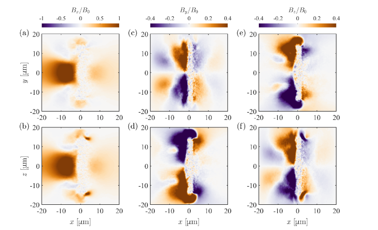
Figure 9: Simulation result for laser beams with a reversed twist ($\varphi=-0.28\pi$). Two-dimensional longitudinal slices at $t=20$ fs of all three components of the time-averaged (averaged over 20 fs output dumps) magnetic field in the 3D PIC simulation with the parameters listed in Table 1. The fields are normalized to $B_{0}=2\pi m_{e}c/|e|\lambda=10.0~{}\rm kT$. $B_{x}$, $B_{y}$, and $B_{z}$ are shown in $(x,y)$-plane (top row) and $(x,z)$-plane (bottom row), respectively. Note that the color scale for $B_{x}$ is different from that for $B_{y}$ and $B_{z}$.

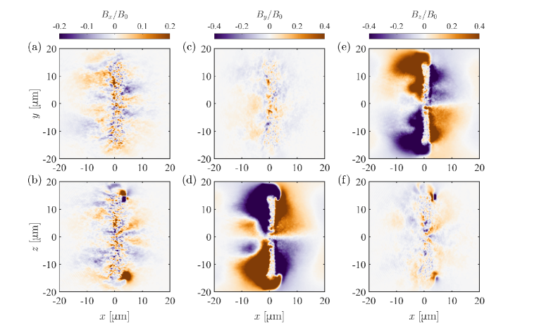
Figure 10: Simulation result for laser beams without a twist ($\varphi=0.0\pi$). Two-dimensional longitudinal slices at $t=20$ fs of all three components of the time-averaged (averaged over 20 fs output dumps) magnetic field in the 3D PIC simulation with the parameters listed in Table 1. The fields are normalized to $B_{0}=2\pi m_{e}c/|e|\lambda=10.0~{}\rm kT$. $B_{x}$, $B_{y}$, and $B_{z}$ are shown in $(x,y)$-plane (top row) and $(x,z)$-plane (bottom row), respectively. Note that the color scale for $B_{x}$ is different from that for $B_{y}$ and $B_{z}$.

Figure 9 and Figure 10 present the two-dimensional longitudinal slices of all three components of the time-averaged (averaged over 20 fs output dumps) magnetic field at $t=20$ fs with the twist angle $\varphi=-0.28\pi$ and $\varphi=0.0\pi$, respectively. When employing laser beams with the opposite twist, the axial magnetic field is reversed, as depicted in Fig. 9. Comparing Fig. 9 and Fig. 6, it is evident that the axially symmetric axial magnetic field $B_{x}$ is reversed, while the transverse magnetic fields $B_{y}$ and $B_{z}$ still exhibit anti-symmetric features. Moreover, the directions of $B_{y}$ in the $(x,y)$-plane and the directions of $B_{z}$ in the $(x,z)$-plane are reverse in Fig. 9 compared to Fig. 6. In Fig. 10, the results suggest that in the absence of a twist, i.e., $\varphi=0$, the axial magnetic field diminishes substantially, while the effect on the transverse magnetic fields is relatively less pronounced due to the existence of a longitudinal current even in the absence of a twist.

The generation of transverse magnetic fields occurs in all three scenarios due to the presence of an axial current induced by the laser pulses. These transverse fields are particularly weak at small radii, underscoring the dominance of the axial magnetic field in governing the magnetic field within the central region. This observation confirms the recognition of a robust mechanism responsible for the generation of axial magnetic fields. It also suggests that the twist parameter can act as a knob for controlling the magnetic field within the central region, similar to the role of the topological charge $l$ for LG beams in the IFE.

4.2 Polarization direction dependency

The polarization direction may play a role in the AM transfer process of our scheme that employs multiple LP Gaussian beams. Intuitively, it may seem that the direction of the transverse laser electric field is crucial for the generation of the azimuthal current. However, it is worth noting that the laser electric field is oscillating, while the current generated by this scheme is quasi-static. The quasi-static current and magnetic field evolve on a much longer time scale than the laser period. The electric field oscillations make it difficult for the laser beams with specific polarization directions to generate the quasi-static azimuthal current with a preferred direction. However, the polarization direction can affect the absorption of laser energy and AM. Based on the absorption characteristics of the plasma, different polarization directions result in different degrees of laser energy absorption within the plasma [76, 77, 78, 79]. This variation could potentially affect the distribution of hot electrons generated within the plasma.

To investigate the impact of the direction of laser polarization, we performed two additional 3D PIC simulations where the polarization direction was deliberately changed compared to that used in the original simulation presented in Section 3. Figure 11 shows the direction of the transverse electric field in the $(y,z)$-plane for each beam, where Fig. 11 (a) shows the original polarization and Fig. 11 (b) and Fig. 11 (c) show the polarization in the two additional simulations. In the original simulation discussed in Section 3, we set the polarization of all four laser beams such that the transverse electric field of each beam in the $(y,z)$-plane was directed along the $y$-axis, as shown in Fig. 11 (a). We will refer to this simulation as “Locked LP₀”. In the first additional simulation, we rotate the polarization direction in every other beam by $\pi/2$. The resulting polarization is shown in Fig. 11 (b). We refer to this simulation as “Locked LP₁”. In the second additional simulation, we introduced random rotation $\xi\in(0,\pi)$ to the original polarization direction for each laser beam. The polarization used in the simulation is shown in Fig. 11 (c). We refer to this simulation as “Random LP”. The purpose of this simulation is to examine whether the multi-beam scheme remains effective even when the linear polarization directions are randomly disordered. It is important to note that in this article we are primarily focused on the effects of the combination of four laser beams with linear polarization on the generation of axial magnetic fields. We do not consider other polarization states. This choice is mainly due to the design of the multi-beam LP laser setup used in most high-power laser systems.

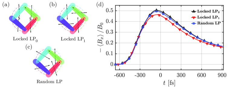
Figure 11: Two-dimensional view of the spatial arrangement and polarization direction of the four laser beams in the $(y,z)$-plane. (a) Locked LP₀ simulation: The linear polarization directions of all four laser beams are along the $y$-axis. (b) Locked LP₁ simulation: A pair of laser beams (cyan and red) are polarized along the $y$-axis, whereas the other pair (green and purple) are polarized along the $z$-axis. (c) Random LP simulation: Random phase shifts $\xi\in(0,\pi)$ are added to the initial polarization directions of the four laser beams, disrupting the regular polarization arrangement of the lasers. (d) Average axial magnetic field within a rectangular volume of length $a=17.9~{}{\upmu\mathrm{m}}$ ($x\in[-19.9,-2.0]~{}{\upmu\mathrm{m}}$), width and height $b$, $c=16~{}{\upmu\mathrm{m}}$ ($y$, $z\in[-8.0,8.0]~{}{\upmu\mathrm{m}}$) as a function of time, where $t=0~{}\rm fs$ is defined as the moment when the lasers leave the simulation space completely. The black, red, and blue solid lines represent the cases of Locked LP₀, Locked LP₁, and Random LP, respectively.

Figure 11 (d) shows the time evolution of the spatially averaged magnetic field for the three different polarization setups: Locked LP₀ (black), Locked LP₁ (red), and Random LP (blue). It is evident that the blue and black curves almost entirely overlap, whereas the red curve is slightly lower than the other two. Based on these results, we infer that co-polarized beams (beams with the same polarization direction) are slightly more favorable for generating the axial magnetic field in our scheme. The result also suggests that even if the polarization directions are somewhat disordered, it will not significantly impact the effectiveness of our scheme. This result is promising for experimental implementation, potentially eliminating the need for deliberate adjustments of initial linear polarization directions.

4.3 Delay dependency

In high-power laser experiments, time delay can pose several challenges that affect the accuracy and reproducibility of experimental outcomes. Specifically, a time delay can cause the interactions between the individual laser beams and the target to occur at different times. This may potentially impact the interaction dynamics. Given the challenges posed by laser synchronization difficulties, it is valuable to examine the role of delays in our scheme. To address this, we examined two different delay scenarios in simulations. In the first scenario, we introduced random delays of up to 250 fs for each of the four laser beams, representing the short delay case. In the second scenario, the delays of four beams are set to 0 fs, 150 fs, 600 fs, and 1000 fs. The delay settings for the two scenarios are illustrated in Fig. 12 (a) and Fig. 12 (b), where the duration of each laser pulse is 600 fs.

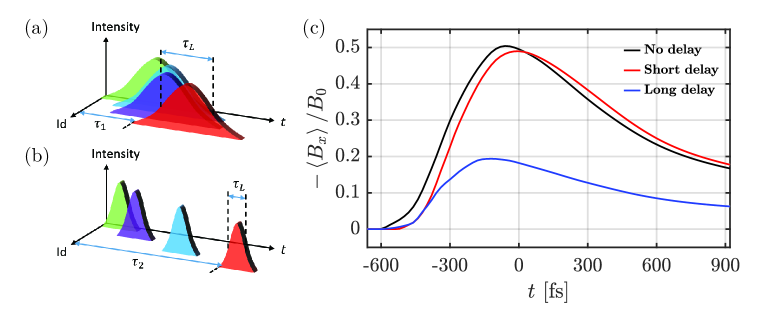
Figure 12: (a) and (b) Two delay scenarios considered in the simulations: the short delay and the long delay. The individual pulse duration is $\tau_{L}=600~{}\rm{fs}$ and the considered delays are $\tau_{1}=250~{}\rm{fs}$ and $\tau_{2}=1~{}\rm{ps}$. Note that the delays are random in the short delay scenario, whereas they are fixed in the long delay scenario. The delays are shown on different time scales. (c) Average axial magnetic field within a rectangular volume of length $a=17.9~{}{\upmu\mathrm{m}}$ ($x\in[-19.9,-2.0]~{}{\upmu\mathrm{m}}$) and width and height $b$, $c=16~{}{\upmu\mathrm{m}}$ ($y$, $z\in[-8.0,8.0]~{}{\upmu\mathrm{m}}$) as a function of time, where $t=0~{}\rm fs$ is defined as the moment when the lasers leave the simulation space completely. The black, red, and blue solid lines represent the cases with no delay, a short delay, and a long delay, respectively.

We find that under the short delay condition in the original simulation, the interaction between the four laser beams and the plasma leads to generation of hot electrons over a greater spatial extent, implying a higher energy transfer efficiency and much faster expansion of the hot electron population. Consequently, in the context of the short delay scenario, various factors, including the strength and spatial range of the axial magnetic field, exhibit a magnitude that is one order higher than those observed under the long delay scenario.

Figure 12 (c) provides the temporal evolution of the spatially averaged axial magnetic field for the two considered delay scenarios. The field for the case without the delay, i.e. the “no delay” curve, is given for reference. We find that the differences between the short delay case and the no delay case are minimal. However, the long delay noticeably reduces the strength of the generated magnetic field compared to the case without the delay. The peak value reaches 40% of the peak value without the delay. Despite this reduction, the magnetic field still reaches the kilotesla range, demonstrating that our scheme remains effective under sufficiently long delay conditions. This provides encouraging prospects for experimental implementation.

4.4 Phase dependency

In multi-beam laser experiments, the phase relationship between different laser beams can produce different synthetic effects. For example, multiple laser beams with a locked phase difference can produce an interference pattern and then improve the efficiency of laser energy conversion into hot electrons [54]. To investigate the effect of phase locking between four beams in our scheme, we introduce random initial phases $\psi_{rd}\in(0,2\pi)$ for each laser beam. Figure 13 (a) shows the time evolution of the spatially averaged magnetic field for two different cases: the locked phase and the random phase. We find that the introduction of random phases does not cause any significant changes. We can conclude that the phase relationship in the simulation did not have a significant effect on the generation of the axial magnetic field. No phase control is required for the combination of multiple laser pulses in our scheme.

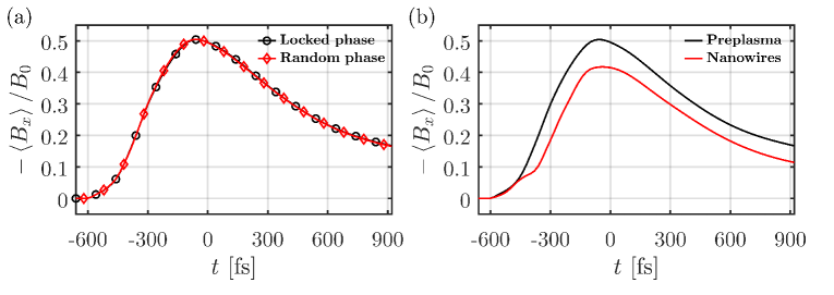
Figure 13: Average axial magnetic field within a cuboid of length $a=17.9~{}{\upmu\mathrm{m}}$ ($x\in[-19.9,-2.0]~{}{\upmu\mathrm{m}}$), width and height $b$, $c=16~{}{\upmu\mathrm{m}}$ ($y$, $z\in[-8.0,8.0]~{}{\upmu\mathrm{m}}$) as a function of time, where $t=0~{}\rm fs$ is defined as the moment when the lasers leave the simulation space completely. (a) The locked phase case is depicted by the solid black line with round markers, while the random phase case is shown as the solid red line with diamond markers. (b) The cases of a solid target with a preplasma and nanowires are given by the black and red solid lines, respectively.

4.5 Solid target with nanowires

After examining the impact of various laser beam parameters, we now shift our focus to the influence of the target shape. In all simulations of this paper, we used a solid target with a preplasma whose parameters can be found in Table 1. The reason for this choice is that a pre-plasma can always be generated by the laser prepulse. With a sufficiently thick preplasma present, the laser energy absorption can be effective. For comparison, we used a solid target with nanowires instead in our previous work [62]. In this section, we present the simulation results obtained using a solid target with nanowires (the setup used in Ref. [62]) while keeping the other parameters the same as in Table 1. To compare the efficiency of magnetic field generation between the case with nanowires and the case with the pre-plasma, the temporal evolution of the spatially averaged magnetic field strength is shown in Fig. 13 (b). The black solid line corresponds to the pre-plasma case, while the red solid line represents the nanowires case. We can see that the nanowires used in our previous work [62] are not a must. Furthermore, it can be inferred that, under our simulation conditions, the use of the chosen preplasma gives better results than nanowires, with an improvement of nearly 10% according to the simulation data. To explore a wider range of parameters of preplasma (like preplasma thickness) or nanowires, more work needs to be done in the future.

5 Comparison with other schemes using CP or LG beams

In previous work on the IFE, CP Gaussian beams were among the first to be studied. For a CP laser beam, each photon carries a maximum SAM of $\sigma_{z}\hbar$, where $\sigma_{z}=+1$ for right-hand and $\sigma_{z}=-1$ for left-hand polarization. Later, vortex beams such as LG beams that are known to carry OAM, were also used to study the IFE. For LG beams, each photon carries an OAM of $(\sigma_{z}+l)\hbar$, where $l$ is the twist index. It is valuable to compare the magnetic field generation in our multi-beam scheme with the magnetic field generation via the IFE using CP or LG beams. According to the model used in previous works [56, 58, 60] and assuming that the laser absorption rate and the electron density are constant in space and time, the following expression for the axial magnetic field can be obtained (see Ref. [60] for more details)

$$B_{z} = \frac{2.25\eta_{\rm abs}I_{0}\tau}{en_{e}\omega w_{0}^{2}}|\psi_{l}|^{2}\times\left[l\left(\frac{|l|w_{0}^{2}}{r^{2}}-2\right)\right.$$ (7)

$$\left.+\sigma_{z}\left(\frac{|l|^{2}w_{0}^{2}}{r^{2}}-4|l|+\frac{4r^{2}}{w_{0}^{2}}-2\right)\right].$$

We have used a Gaussian temporal pulse shape, with $\tau$ being the temporal full width at half maximum (FWHM). In Eq. 7, $n_{e}$ is the electron density, $\eta_{\rm abs}$ is the laser energy absorption fraction per unit length, $I_{0}$ is the peak intensity and $w_{0}$ is the beam waist. Using reasonable assumptions, Longman [60] obtains the absorption rate as $\eta_{\rm abs}=n_{e}/(2n_{c}c\tau)$, then estimates the peak axial magnetic field strength of the $|\sigma_{z}|=1$, $|l|=0$ and $|\sigma_{z}|=0$, $|l|=1$ modes for $\tau\gtrsim 100~{}\rm fs$ and $n_{e}\gtrsim 0.01~{}n_{c}$ as $|B|_{\rm max}\approx(P~{}[{\rm TW}]\lambda^{3}~{}[{\upmu\mathrm{m}}]/w_{0}^{4}~{}[{\upmu\mathrm{m}}])~{}[10~{}\rm{kT}]$, where $P=0.75\pi I_{0}w_{0}^{2}$ is the laser power and $\eta_{\rm abs}\approx 0.2~{}\rm mm^{-1}$ is the value for the underdense plasma. The axial magnetic field $|B|_{\rm max}$ shows a fourth power dependence on the laser beam waist $w_{0}$. Meanwhile, under our high density plasma conditions, the absorption rate is expected to reach $\eta_{\rm abs}\simeq\eta_{0}\approx 32.3~{}\rm mm^{-1}$. Despite having a high absorption rate in our scenario, the total absorption may be reduced due to a limited interaction length of the laser absorption process caused by the presence of the high density plasma that is opaque to the laser beams.

To make a quantitative comparison, we ran two 3D PIC simulations: one with a single CP Gaussian beam and another with a single LP LG beam. In these simulations, we set the laser parameters such that the laser energy is equal to the laser energy in the four beams from Table 1. Additionally, we choose the beam waist radius to be equal to the beam offset ($w_{0}=f_{0}$) in Fig. 2 (b). This choice was made to ensure the transverse extension of the generated magnetic field matches that for the four-beam setup. Note that previous studies indicated that different laser modes with different values of $l$ and $\sigma_{z}$ produce radial magnetic field distributions with the intense region confined within $1.5w_{0}$, as shown in Ref. [60]. It is worth pointing out that the magnetic field has a similar radial distribution for both the CP Gaussian beam ($|\sigma_{z}|=1$, $|l|=0$) and the LP LG beam ($|\sigma_{z}|=0$, $|l|=1$). Inserting these parameters into the expression of $|B|_{\rm max}$ above, we can estimate the axial magnetic field strength to be about 0.4 kT. In Fig. 14, the logarithmic plots show the time evolution of the spatially averaged axial magnetic field for the three schemes mentioned here. The black curve represents the four LP Gaussian beams scenario. The red and blue curves represent the cases of a single LP LG and single CP Gaussian beam, respectively. It can be seen that the latter two have magnetic field strengths about two orders of magnitude lower than the former. In our simulations, the single CP Gaussian beam performs less effectively, while our multi-beam scheme shows distinct advantages under the same energy condition.

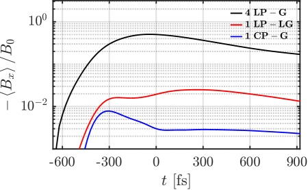
Figure 14: Average axial magnetic field within a rectangular volume of length $a=17.9~{}{\upmu\mathrm{m}}$ ($x\in[-19.9,-2.0]~{}{\upmu\mathrm{m}}$), width and height $b$, $c=16~{}{\upmu\mathrm{m}}$ ($y$, $z\in[-8.0,8.0]~{}{\upmu\mathrm{m}}$) as a function of time, where $t=0~{}\rm fs$ is defined as the moment when the lasers leave the simulation space completely. The black, red and blue solid lines represent the cases of four LP Gaussian laser beams, single LP LG mode laser, and single CP Gaussian mode laser, respectively.

6 Summary and discussion

In summary, we have presented a comprehensive computational study of a setup where a strong axial magnetic field is generated in an interaction of multiple conventional laser beams with a target. The magnetic field strength in the considered setup reaches 10 kT, with the strong field occupying tens of thousands of cubic microns. The field persists on a ps time scale. Although a CP Gaussian laser beam and an LG laser beam can carry intrinsic AM, native beams at current high-power laser systems are not CP or LG beams, but rather conventional LP beams. Moreover, the design kJ-level PW-class laser systems is such that they are composed of multiple LP beams. This consideration motivated the development of our scheme that uses four laser beams with a twist in the pointing direction (shown in Fig. 1) to achieve net OAM.

The key role of the AM carried by these laser beams in initiating the magnetic field generation process has been established. The simulations examine various aspects, including the distribution of the axial magnetic field, azimuthal current, and electron and ion OAM densities. Dependencies on factors such as twist angle, polarization direction, delay, phase, and target structures have also been extensively studied. Our study has validated the effectiveness of this approach under various conditions, confirming its robustness and practical feasibility. In particular, the twist angle of the laser pulse emerges as a critical driver for maintaining the azimuthal plasma current that maintains the orientation of the magnetic field. Furthermore, the PIC simulations and supporting theory indicate that the twist angle serves as a convenient control knob for adjusting the direction and magnitude of the axial magnetic field.

When compared to other schemes using CP or LG beams, the multi-beam configuration has several advantages. In particular, our approach requires only an LP Gaussian beam configuration, making it suitable for advanced high-power, high-intensity multi-beam laser systems such as the upcoming major upgrade, SG-ii@ UP. Despite the challenges associated with pointing directions, the results underscore the feasibility of achieving a strong and sustained axial magnetic field using thoughtfully designed multi-beam setups. These studies contribute significantly to the understanding of laser-plasma interactions and expand the capabilities of high-power laser systems. The results may provide new opportunities to study the kT-scale magnetic field where the magnetic field energy density is greater than $10^{11}~{}\rm{J\cdot m}^{-3}$ which is usually the baseline in HED science. Other studies of strong magnetic field physics can also be expected.

Data availability statement

Data available on request from the authors. The data that support the findings of this study are available from the corresponding author upon reasonable request.

References

- [1] C. Plechaty, R. Presura, S. Stein, D. Martinez, S. Neff, V. Ivanov, and Y. Stepanenko, “Penetration of a laser-produced plasma across an applied magnetic field,” High Energy Density Physics, vol. 6, no. 2, pp. 258–261, 2010. ICHED 2009 - 2nd International Conference on High Energy Density Physics.
- [2] B. Albertazzi, A. Ciardi, M. Nakatsutsumi, T. Vinci, J. Béard, R. Bonito, J. Billette, M. Borghesi, Z. Burkley, S. N. Chen, T. E. Cowan, T. Herrmannsdörfer, D. P. Higginson, F. Kroll, S. A. Pikuz, K. Naughton, L. Romagnani, C. Riconda, G. Revet, R. Riquier, H.-P. Schlenvoigt, I. Y. Skobelev, A. Faenov, A. Soloviev, M. Huarte-Espinosa, A. Frank, O. Portugall, H. Pépin, and J. Fuchs, “Laboratory formation of a scaled protostellar jet by coaligned poloidal magnetic field,” Science, vol. 346, no. 6207, pp. 325–328, 2014.
- [3] D. Schaeffer, W. Fox, D. Haberberger, G. Fiksel, A. Bhattacharjee, D. Barnak, S. Hu, K. Germaschewski, and R. Follett, “High-mach number, laser-driven magnetized collisionless shocks,” Physics of Plasmas, vol. 24, Dec. 2017.
- [4] T. Byvank, J. T. Banasek, W. M. Potter, J. B. Greenly, C. E. Seyler, and B. R. Kusse, “Applied axial magnetic field effects on laboratory plasma jets: Density hollowing, field compression, and azimuthal rotation,” Physics of Plasmas, vol. 24, 12 2017.
- [5] K. Matsuo, N. Higashi, N. Iwata, S. Sakata, S. Lee, T. Johzaki, H. Sawada, Y. Iwasa, K. F. F. Law, H. Morita, Y. Ochiai, S. Kojima, Y. Abe, M. Hata, T. Sano, H. Nagatomo, A. Sunahara, A. Morace, A. Yogo, M. Nakai, H. Sakagami, T. Ozaki, K. Yamanoi, T. Norimatsu, Y. Nakata, S. Tokita, J. Kawanaka, H. Shiraga, K. Mima, H. Azechi, R. Kodama, Y. Arikawa, Y. Sentoku, and S. Fujioka, “Petapascal pressure driven by fast isochoric heating with a multipicosecond intense laser pulse.,” Physical review letters, vol. 124 3, p. 035001, 2019.
- [6] L. Yi, B. Shen, A. Pukhov, and T. Fülöp, “Relativistic magnetic reconnection driven by a laser interacting with a micro-scale plasma slab.,” Nat Commun, vol. 9 1, p. 1601, 2018.
- [7] Y. Ping, J. Zhong, X. Wang, G. Zhao, Y. Li, and X.-T. He, “Reconnection rate and multi-scale relativistic magnetic reconnection driven by ultra-intense lasers,” Plasma Physics and Controlled Fusion, vol. 63, p. 085012, jun 2021.
- [8] A. E. Raymond, C. F. Dong, A. McKelvey, C. Zulick, N. Alexander, A. Bhattacharjee, P. T. Campbell, H. Chen, V. Chvykov, E. Del Rio, P. Fitzsimmons, W. Fox, B. Hou, A. Maksimchuk, C. Mileham, J. Nees, P. M. Nilson, C. Stoeckl, A. G. R. Thomas, M. S. Wei, V. Yanovsky, K. Krushelnick, and L. Willingale, “Relativistic-electron-driven magnetic reconnection in the laboratory,” Phys. Rev. E, vol. 98, p. 043207, Oct 2018.
- [9] K. F. F. Law, Y. Abe, A. Morace, Y. Arikawa, S. Sakata, S. Lee, K. Matsuo, H. Morita, Y. Ochiai, C. Liu, A. Yogo, K. Okamoto, D. Golovin, M. Ehret, T. Ozaki, M. Nakai, Y. Sentoku, J. J. Santos, E. d’Humières, P. Korneev, and S. Fujioka, “Relativistic magnetic reconnection in laser laboratory for testing an emission mechanism of hard-state black hole system,” Phys. Rev. E, vol. 102, p. 033202, Sep 2020.
- [10] A. Arefiev, T. Toncian, and G. Fiksel, “Enhanced proton acceleration in an applied longitudinal magnetic field,” New Journal of Physics, vol. 18, p. 105011, oct 2016.
- [11] S. X. Luan, W. Yu, F. Y. Li, D. Wu, Z. M. Sheng, M. Y. Yu, and J. Zhang, “Publisher’s note: Laser propagation in dense magnetized plasma [phys. rev. e 94, 053207 (2016)],” Phys. Rev. E, vol. 94, p. 069903, Dec 2016.
- [12] T. Sano, Y. Tanaka, N. Iwata, M. Hata, K. Mima, M. Murakami, and Y. Sentoku, “Broadening of cyclotron resonance conditions in the relativistic interaction of an intense laser with overdense plasmas,” Phys. Rev. E, vol. 96, p. 043209, Oct 2017.
- [13] K. Li and W. Yu, “Laser propagation in a highly magnetized over-dense plasma,” Physics of Plasmas, vol. 27, p. 102712, 10 2020.
- [14] K. Li and W. Yu, “Optical probing of magnet-induced transparent over-dense plasma in a whistler mode,” Physics of Plasmas, vol. 30, p. 092105, 09 2023.
- [15] D. Liu, W. Fan, L. Shan, C. Tian, B. Bi, F. Zhang, Z. Yuan, W. Wang, H. Liu, L. Yang, L. Meng, L. Cao, W. Zhou, and Y. Gu, “Ab initio simulations for expanded gold fluid in metal-nonmetal transition regime,” Physics of Plasmas, vol. 26, p. 122705, 12 2019.
- [16] K. Higuchi, D. B. Hamal, and M. Higuchi, “Nonperturbative description of the butterfly diagram of energy spectra for materials immersed in a magnetic field,” Phys. Rev. B, vol. 97, p. 195135, May 2018.
- [17] F. Herlach and N. Miura, High magnetic fields: Science and technology. World Scientific Publishing Company, 01 2006.
- [18] D. J. Strozzi, M. Tabak, D. J. Larson, L. Divol, A. J. Kemp, C. Bellei, M. M. Marinak, and M. H. Key, “Fast-ignition transport studies: Realistic electron source, integrated particle-in-cell and hydrodynamic modeling, imposed magnetic fields,” Physics of Plasmas, vol. 19, p. 072711, 07 2012.
- [19] R. Z. Sagdeev, “Cooperative phenomena and shock waves in collisionless plasmas,” Rev. Plasma Phys. (USSR)(Engl. Transl.), vol. 4, 1 1966.
- [20] W. Yao, A. Fazzini, S. N. Chen, K. Burdonov, P. Antici, J. Béard, S. Bolaños, A. Ciardi, R. Diab, E. D. Filippov, S. Kisyov, V. Lelasseux, M. Miceli, Q. Moreno, V. Nastasa, S. Orlando, S. Pikuz, D. C. Popescu, G. Revet, X. Ribeyre, E. d’Humières, and J. Fuchs, “Detailed characterization of a laboratory magnetized supercritical collisionless shock and of the associated proton energization,” Matter and Radiation at Extremes, vol. 7, p. 014402, 12 2021.
- [21] A. V. Kuznetsov, T. Z. Esirkepov, F. F. Kamenets, and S. V. Bulanov, “Efficiency of ion acceleration by a relativistically strong laser pulse in an underdense plasma,” Plasma Physics Reports, vol. 27, pp. 211–220, 2001.
- [22] Y. Fukuda, A. Y. Faenov, M. Tampo, T. A. Pikuz, T. Nakamura, M. Kando, Y. Hayashi, A. Yogo, H. Sakaki, T. Kameshima, A. S. Pirozhkov, K. Ogura, M. Mori, T. Z. Esirkepov, J. Koga, A. S. Boldarev, V. A. Gasilov, A. I. Magunov, T. Yamauchi, R. Kodama, P. R. Bolton, Y. Kato, T. Tajima, H. Daido, and S. V. Bulanov, “Energy increase in multi-mev ion acceleration in the interaction of a short pulse laser with a cluster-gas target,” Phys. Rev. Lett., vol. 103, p. 165002, Oct 2009.
- [23] T. Nakamura, S. V. Bulanov, T. Z. Esirkepov, and M. Kando, “High-energy ions from near-critical density plasmas via magnetic vortex acceleration,” Phys. Rev. Lett., vol. 105, p. 135002, Sep 2010.
- [24] S. S. Bulanov, E. Esarey, C. B. Schroeder, W. P. Leemans, S. V. Bulanov, D. Margarone, G. Korn, and T. Haberer, “Helium-3 and helium-4 acceleration by high power laser pulses for hadron therapy,” Phys. Rev. ST Accel. Beams, vol. 18, p. 061302, Jun 2015.
- [25] J. Park, S. S. Bulanov, J. Bin, Q. Ji, S. Steinke, J.-L. Vay, C. G. R. Geddes, C. B. Schroeder, W. P. Leemans, T. Schenkel, and E. Esarey, “Ion acceleration in laser generated megatesla magnetic vortex,” Physics of Plasmas, vol. 26, p. 103108, 10 2019.
- [26] J. X. Gong, L. H. Cao, K. Q. Pan, K. D. Xiao, D. Wu, C. Y. Zheng, Z. J. Liu, and X. T. He, “Enhancement of proton acceleration by a right-handed circularly polarized laser interaction with a cone target exposed to a longitudinal magnetic field,” Physics of Plasmas, vol. 24, p. 053109, 05 2017.
- [27] Y. Gu and S. V. Bulanov, “Magnetic field annihilation and charged particle acceleration in ultra-relativistic laser plasmas,” High Power Laser Science and Engineering, vol. 9, 2021.
- [28] B. Albertazzi, J. Béard, A. Ciardi, T. Vinci, J. Albrecht, J. Billette, T. Burris-Mog, S. N. Chen, D. Da Silva, S. Dittrich, T. Herrmannsdörfer, B. Hirardin, F. Kroll, M. Nakatsutsumi, S. Nitsche, C. Riconda, L. Romagnagni, H.-P. Schlenvoigt, S. Simond, E. Veuillot, T. E. Cowan, O. Portugall, H. Pépin, and J. Fuchs, “Production of large volume, strongly magnetized laser-produced plasmas by use of pulsed external magnetic fields,” Review of Scientific Instruments, vol. 84, p. 043505, 04 2013.
- [29] R. V. Shapovalov, G. Brent, R. Moshier, M. Shoup, R. B. Spielman, and P.-A. Gourdain, “Design of 30-t pulsed magnetic field generator for magnetized high-energy-density plasma experiments,” Phys. Rev. Accel. Beams, vol. 22, p. 080401, Aug 2019.
- [30] H. P, H. GY, W. YL, T. HB, Z. ZC, and Z. J., “Pulsed magnetic field device for laser plasma experiments at shenguang-ii laser facility. rev sci instrum.,” Nat Commun, vol. 91 1, p. 014703, 2020.
- [31] R. J. Mason and M. Tabak, “Magnetic field generation in high-intensity-laser–matter interactions,” Phys. Rev. Lett., vol. 80, pp. 524–527, Jan 1998.
- [32] M. Roth and M. S. Schollmeier, “Ion acceleration - target normal sheath acceleration,” arXiv: Accelerator Physics, 2016.
- [33] U. Wagner, M. Tatarakis, A. Gopal, F. N. Beg, E. L. Clark, A. E. Dangor, R. G. Evans, M. G. Haines, S. P. D. Mangles, P. A. Norreys, M.-S. Wei, M. Zepf, and K. Krushelnick, “Laboratory measurements of magnetic fields generated during high-intensity laser interactions with dense plasmas,” Phys. Rev. E, vol. 70, p. 026401, Aug 2004.
- [34] Y. C. Yang, T. W. Huang, M. Y. Yu, K. Jiang, and C. T. Zhou, “Generation of jet-forming plasma bunch with gigagauss axial magnetic field from impact of linearly polarized laser on microtube targets,” Physics of Plasmas, vol. 30, p. 112103, 11 2023.
- [35] M.-A. H. Zosa, Y. J. Gu, and M. Murakami, “100-kT magnetic field generation using paisley targets by femtosecond laser–plasma interactions,” Applied Physics Letters, vol. 120, p. 132403, 03 2022.
- [36] D. Nakamura, A. Ikeda, H. Sawabe, Y. H. Matsuda, and S. Takeyama, “Record indoor magnetic field of 1200 T generated by electromagnetic flux-compression,” Review of Scientific Instruments, vol. 89, p. 095106, 09 2018.
- [37] A. B. Sefkow, S. A. Slutz, J. M. Koning, M. M. Marinak, K. J. Peterson, D. B. Sinars, and R. A. Vesey, “Design of magnetized liner inertial fusion experiments using the Z facilitya),” Physics of Plasmas, vol. 21, p. 072711, 07 2014.
- [38] O. V. Gotchev, P. Y. Chang, J. P. Knauer, D. D. Meyerhofer, O. Polomarov, J. Frenje, C. K. Li, M. J.-E. Manuel, R. D. Petrasso, J. R. Rygg, F. H. Séguin, and R. Betti, “Laser-driven magnetic-flux compression in high-energy-density plasmas,” Phys. Rev. Lett., vol. 103, p. 215004, Nov 2009.
- [39] J. D. Moody, “Boosting inertial-confinement-fusion yield with magnetized fuel,” Physics, vol. 14, 2021.
- [40] J. J. Santos, M. Bailly-Grandvaux, L. Giuffrida, P. Forestier-Colleoni, S. Fujioka, Z. Zhang, P. Korneev, R. Bouillaud, S. Dorard, D. Batani, M. Chevrot, J. E. Cross, R. Crowston, J.-L. Dubois, J. Gazave, G. Gregori, E. d’Humières, S. Hulin, K. Ishihara, S. Kojima, E. Loyez, J.-R. Marquès, A. Morace, P. Nicolaï, O. Peyrusse, A. Poyé, D. Raffestin, J. Ribolzi, M. Roth, G. Schaumann, F. Serres, V. T. Tikhonchuk, P. Vacar, and N. Woolsey, “Laser-driven platform for generation and characterization of strong quasi-static magnetic fields,” New Journal of Physics, vol. 17, p. 083051, aug 2015.
- [41] I. V. Kochetkov, N. Bukharskii, M. Ehret, Y. Abe, K. F. F. Law, V. Ospina-Bohórquez, J. J. Santos, S. Fujioka, G. Schaumann, B. Zielbauer, A. P. Kuznetsov, and P. A. Korneev, “Neural network analysis of quasistationary magnetic fields in microcoils driven by short laser pulses,” Scientific Reports, vol. 12, 2022.
- [42] B. K. Russell, P. T. Campbell, Q. Qian, J. A. Cardarelli, S. S. Bulanov, S. V. Bulanov, G. M. Grittani, D. Seipt, L. Willingale, and A. G. R. Thomas, “Ultrafast relativistic electron probing of extreme magnetic fields,” Physics of Plasmas, vol. 30, p. 093105, 09 2023.
- [43] B. Zhu, Z. Zhang, C. Liu, D. Yuan, W. Jiang, H. Wei, F. Li, Y. Zhang, B. Han, L. Cheng, S. Li, J. Zhong, X. Yuan, B. Tong, W. Sun, Z. Fang, C. Wang, Z. Xie, N. Hua, R. Wu, Z. Qiao, G. Liang, B. Zhu, J. Zhu, S. Fujioka, and Y. Li, “Observation of Zeeman splitting effect in a laser-driven coil,” Matter and Radiation at Extremes, vol. 7, p. 024402, 02 2022.
- [44] J. L. Peebles, J. R. Davies, D. H. Barnak, F. Garcia-Rubio, P. V. Heuer, G. Brent, R. Spielman, and R. Betti, “An assessment of generating quasi-static magnetic fields using laser-driven “capacitor” coils,” Physics of Plasmas, vol. 29, p. 080501, 08 2022.
- [45] G. Liao, Y. Li, B. Zhu, Y. Li, F. Li, M. Li, X. Wang, Z. Zhang, S. He, W. Wang, F. Lu, F. Zhang, L. Yang, K. Zhou, N. Xie, W. Hong, Y. Gu, Z. Zhao, B. Zhang, and J. Zhang, “Proton radiography of magnetic fields generated with an open-ended coil driven by high power laser pulses,” Matter and Radiation at Extremes, vol. 1, pp. 187–191, 07 2016.
- [46] D. Strickland and G. Mourou, “Compression of amplified chirped optical pulses,” Optics Communications, vol. 56, no. 3, pp. 219–221, 1985.
- [47] M. Tatarakis, I. Watts, F. N. Beg, E. L. Clark, A. E. Dangor, A. Gopal, M. G. Haines, P. A. Norreys, U. Wagner, M.-S. Wei, M. Zepf, and K. Krushelnick, “Measuring huge magnetic fields,” Nature, vol. 415, pp. 280–280, Jan 2002.
- [48] X. X. Li, R. J. Cheng, Q. Wang, D. J. Liu, S. Y. Lv, Z. M. Huang, S. T. Zhang, X. M. Li, Z. J. Chen, Q. Wang, Z. J. Liu, L. H. Cao, C. Y. Zheng, and X. T. He, “Anomalous staged hot-electron acceleration by two-plasmon decay instability in magnetized plasmas,” Phys. Rev. E, vol. 108, p. L053201, Nov 2023.
- [49] D. J. Stark, T. Toncian, and A. V. Arefiev, “Enhanced multi-mev photon emission by a laser-driven electron beam in a self-generated magnetic field,” Phys. Rev. Lett., vol. 116, p. 185003, May 2016.
- [50] C. N. Danson, C. Haefner, J. Bromage, T. Butcher, J.-C. F. Chanteloup, E. A. Chowdhury, A. Galvanauskas, L. A. Gizzi, J. Hein, D. I. Hillier, and et al., “Petawatt and exawatt class lasers worldwide,” High Power Laser Science and Engineering, vol. 7, p. e54, 2019.
- [51] J. Kawanaka, N. Miyanaga, H. Azechi, T. Kanabe, T. Jitsuno, K. Kondo, Y. Fujimoto, N. Morio, S. Matsuo, Y. Kawakami, R. Mizoguchi, K. Tauchi, M. Yano, S. Kudo, and Y. Ogura, “3.1-kj chirped-pulse power amplification in the lfex laser,” Journal of Physics: Conference Series, vol. 112, p. 032006, may 2008.
- [52] J. K. Crane, G. Tietbohl, P. Arnold, E. S. Bliss, C. Boley, G. Britten, G. Brunton, W. Clark, J. W. Dawson, S. Fochs, R. Hackel, C. Haefner, J. Halpin, J. Heebner, M. Henesian, M. Hermann, J. Hernandez, V. Kanz, B. McHale, J. B. McLeod, H. Nguyen, H. Phan, M. Rushford, B. Shaw, M. Shverdin, R. Sigurdsson, R. Speck, C. Stolz, D. Trummer, J. Wolfe, J. N. Wong, G. C. Siders, and C. P. J. Barty, “Progress on converting a nif quad to eight, petawatt beams for advanced radiography,” Journal of Physics: Conference Series, vol. 244, p. 032003, aug 2010.
- [53] D. Batani, M. Koenig, J. L. Miquel, J. E. Ducret, E. d’Humieres, S. Hulin, J. Caron, J. L. Feugeas, P. Nicolai, V. Tikhonchuk, L. Serani, N. Blanchot, D. Raffestin, I. Thfoin-Lantuejoul, B. Rosse, C. Reverdin, A. Duval, F. Laniesse, A. Chancé, D. Dubreuil, B. Gastineau, J. C. Guillard, F. Harrault, D. Lebœuf, J.-M. L. Ster, C. Pès, J.-C. Toussaint, X. Leboeuf, L. Lecherbourg, C. I. Szabo, J.-L. Dubois, and F. Lubrano-Lavaderci, “Development of the petawatt aquitaine laser system and new perspectives in physics,” Physica Scripta, vol. 2014, p. 014016, may 2014.
- [54] A. Morace, N. Iwata, Y. Sentoku, K. Mima, Y. Arikawa, A. Yogo, A. Andreev, S. Tosaki, X. Vaisseau, Y. Abe, S. Kojima, S. Sakata, M. Hata, S. Lee, K. Matsuo, N. Kamitsukasa, T. Norimatsu, J. Kawanaka, S. Tokita, N. Miyanaga, H. Shiraga, Y. Sakawa, M. Nakai, H. Nishimura, H. Azechi, S. Fujioka, and R. Kodama, “Enhancing laser beam performance by interfering intense laser beamlets,” Nature Communications, vol. 10, p. 2995, Jul 2019.
- [55] J. Zhu, J. Zhu, X. Li, B. Zhu, W. Ma, X. Lu, W. Fan, Z. Liu, S. Zhou, G. Xu, and et al., “Status and development of high-power laser facilities at the nlhplp,” High Power Laser Science and Engineering, vol. 6, p. e55, 2018.
- [56] M. G. Haines, “Generation of an axial magnetic field from photon spin,” Phys. Rev. Lett., vol. 87, p. 135005, Sep 2001.
- [57] L. Allen, M. W. Beijersbergen, R. J. C. Spreeuw, and J. P. Woerdman, “Orbital angular momentum of light and the transformation of laguerre-gaussian laser modes,” Phys. Rev. A, vol. 45, pp. 8185–8189, Jun 1992.
- [58] S. Ali, J. R. Davies, and J. T. Mendonca, “Inverse faraday effect with linearly polarized laser pulses,” Phys. Rev. Lett., vol. 105, p. 035001, Jul 2010.
- [59] R. Nuter, P. Korneev, E. Dmitriev, I. Thiele, and V. T. Tikhonchuk, “Gain of electron orbital angular momentum in a direct laser acceleration process,” Phys. Rev. E, vol. 101, p. 053202, May 2020.
- [60] A. Longman and R. Fedosejevs, “Kilo-tesla axial magnetic field generation with high intensity spin and orbital angular momentum beams,” Phys. Rev. Res., vol. 3, p. 043180, Dec 2021.
- [61] Z. Li, Y. Leng, and R. Li, “Further development of the short-pulse petawatt laser: Trends, technologies, and bottlenecks,” Laser & Photonics Reviews, vol. n/a, no. n/a, p. 2100705, 2022.
- [62] Y. Shi, A. Arefiev, J. X. Hao, and J. Zheng, “Efficient generation of axial magnetic field by multiple laser beams with twisted pointing directions,” Phys. Rev. Lett., vol. 130, p. 155101, Apr 2023.
- [63] K. Y. Bliokh, F. J. Rodríguez-Fortuño, F. Nori, and A. V. Zayats, “Spin–orbit interactions of light,” Nature Photonics, vol. 9, no. 12, pp. 796–808, 2015.
- [64] C. Liu, B. Shen, X. Zhang, Y. Shi, L. Ji, W. Wang, L. Yi, L. Zhang, T. Xu, Z. Pei, and Z. Xu, “Generation of gamma-ray beam with orbital angular momentum in the qed regime,” Physics of Plasmas, vol. 23, no. 9, p. 093120, 2016.
- [65] Y.-Y. Chen, J.-X. Li, K. Z. Hatsagortsyan, and C. H. Keitel, “-ray beams with large orbital angular momentum via nonlinear compton scattering with radiation reaction,” Phys. Rev. Lett., vol. 121, p. 074801, Aug 2018.
- [66] Y.-Y. Chen, K. Z. Hatsagortsyan, and C. H. Keitel, “Generation of twisted -ray radiation by nonlinear thomson scattering of twisted light,” Matter and Radiation at Extremes, vol. 4, no. 2, p. 024401, 2019.
- [67] T. Arber, K. Bennett, C. Brady, A. Lawrence-Douglas, M. Ramsay, N. Sircombe, P. Gillies, R. Evans, H. Schmitz, A. Bell, and C. Ridgers, “Contemporary particle-in-cell approach to laser-plasma modelling,” Plasma Physics and Controlled Fusion, vol. 57, no. 11, p. 113001, 2015.
- [68] J. Griff-McMahon, S. Malko, V. Valenzuela-Villaseca, C. Walsh, G. Fiksel, M. J. Rosenberg, D. B. Schaeffer, and W. Fox, “Measurements of extended magnetic fields in laser-solid interaction,” 2023. arXiv:2310.18592.
- [69] G. Pérez-Callejo, C. Vlachos, C. A. Walsh, R. Florido, M. Bailly-Grandvaux, X. Vaisseau, F. Suzuki-Vidal, C. McGuffey, F. N. Beg, P. Bradford, V. Ospina-Bohórquez, D. Batani, D. Raffestin, A. Colaïtis, V. Tikhonchuk, A. Casner, M. Koenig, B. Albertazzi, R. Fedosejevs, N. Woolsey, M. Ehret, A. Debayle, P. Loiseau, A. Calisti, S. Ferri, J. Honrubia, R. Kingham, R. C. Mancini, M. A. Gigosos, and J. J. Santos, “Cylindrical implosion platform for the study of highly magnetized plasmas at laser megajoule,” Phys. Rev. E, vol. 106, p. 035206, Sep 2022.
- [70] J. D. Jackson, Electrodynamics. Wiley Online Library, 1975.
- [71] Y. Shi, J. Vieira, R. Trines, R. Bingham, B. Shen, and R. J. Kingham, “Magnetic field generation in plasma waves driven by copropagating intense twisted lasers.,” Physical review letters, vol. 121 14, p. 145002, 2018.
- [72] T. V. Liseykina, S. V. Popruzhenko, and A. Macchi, “Inverse faraday effect driven by radiation friction,” New Journal of Physics, vol. 18, p. 072001, jul 2016.
- [73] F. Brunel, “Anomalous absorption of high intensity subpicosecond laser pulses,” The Physics of Fluids, vol. 31, no. 9, pp. 2714–2719, 1988.
- [74] M. C. Levy, S. C. Wilks, M. Tabak, S. B. Libby, and M. G. Baring, “Petawatt laser absorption bounded,” Nature Communications, vol. 5, p. 4149, Jun 2014.
- [75] A. Grassi, M. Grech, F. Amiranoff, A. Macchi, and C. Riconda, “Radiation-pressure-driven ion weibel instability and collisionless shocks,” Phys. Rev. E, vol. 96, p. 033204, Sep 2017.
- [76] D. D. Meyerhofer, H. Chen, J. A. Delettrez, B. Soom, S. Uchida, and B. Yaakobi, “Resonance absorption in high‐intensity contrast, picosecond laser–plasma interactions*,” Physics of Fluids B: Plasma Physics, vol. 5, pp. 2584–2588, 07 1993.
- [77] J. S. Pearlman, J. J. Thomson, and C. E. Max, “Polarization-dependent absorption of laser radiation incident on dense-plasma planar targets,” Phys. Rev. Lett., vol. 38, pp. 1397–1400, Jun 1977.
- [78] J. S. Pearlman and M. K. Matzen, “Angular dependence of polarization-related laser-plasma absorption processes,” Phys. Rev. Lett., vol. 39, pp. 140–142, Jul 1977.
- [79] J. E. Balmer and T. P. Donaldson, “Resonance absorption of 1.06- m laser radiation in laser-generated plasma,” Phys. Rev. Lett., vol. 39, pp. 1084–1087, Oct 1977.