MS-RMA-20-xxxxx Jia et al. Markdown Pricing Under Unknown Parametric Demand

Markdown Pricing Under an Unknown Parametric Demand Model Consider a single-product revenue-maximization problem where the seller monotonically decreases the price in $n$ rounds with an unknown demand model coming from a given family. Without monotonicity, the minimax regret is $\tilde{O}(n^{2/3})$ for the Lipschitz demand family (Kleinberg and Leighton 2003) and $\tilde{O}(n^{1/2})$ for a general class of parametric demand models (Broder and Rusmevichientong 2012). With monotonicity, the minimax regret is $\tilde{O}(n^{3/4})$ if the revenue function is Lipschitz and unimodal (Chen 2021, Jia et al. 2021). However, the minimax regret for parametric families remained open. In this work, we provide a complete settlement for this fundamental problem. We introduce the crossing number to measure the complexity of a family of demand functions. In particular, the family of degree-$k$ polynomials has a crossing number $k$. Based on conservatism under uncertainty, we present (i) a policy with an optimal $\Theta(\log^{2}n)$ regret for families with crossing number $k=0$, and (ii) another policy with an optimal $\tilde{\Theta}(n^{k/(k+1)})$ regret when $k\geq 1$. These bounds are asymptotically higher than the $\tilde{O}(\log n)$ and $\tilde{\Theta}(\sqrt{n})$ minimax regret for the same families without the monotonicity constraint (Broder and Rusmevichientong 2012).

Su Jia Center of Data Science for Enterprise and Society, Cornell University Andrew A. Li, R. Ravi Tepper School of Business, Carnegie Mellon University

markdown pricing, multi-armed bandits, demand learning, parametric demand models

1 Introduction

A core challenge in revenue management involves implementing dynamic pricing in the face of uncertain demand, particularly when introducing new products. A critical aspect overlooked in the current literature is the direction of price changes. Traditional models may involve sellers strategically raising prices to maximize earnings per unit, a strategy considered reasonable when the anticipated reduction in demand is relatively low. However, in practice, there is a disparity in the treatment of price increases and price decreases (markdowns). This is because the negative impact posed by price increases cannot always be offset by the additional per-unit gain. For example, price increases may contribute to a perception of manipulation and adversely affect the seller’s ratings. More concretely, through an analysis of the online menu prices of a group of restaurants, Luca and Reshef (2021) found that

“a price increase of 1% leads to a decrease of 3% – 5% in the average rating.”

As a result, sellers may incur an implicit penalty for implementing price increases. We study the fundamental aspects of this directional asymmetry in price changes by imposing a monotonicity constraint. The objective is to identify a markdown policy - a policy that never increases the price - to maximize revenue in the presence of an unknown demand model.

Despite its practical importance, markdown pricing under demand uncertainty is less well understood, compared to the unconstrained pricing problem (i.e., without the monotonicity constraint). Existing work only focused on nonparametric models. Chen (2021) and Jia et al. (2021) showed that unimodality and Lipschitzness in the revenue function (i.e., the product of price and mean demand) are sufficient and necessary to achieve sublinear regret. They proposed a policy with an optimal $\tilde{O}(n^{3/4})$ regret, i.e., loss due to not knowing the true model. In addition, if the demand function is twice continuously differentiable, the regret can be improved to $\tilde{O}(n^{5/7})$; see Theorem 2 of Jia et al. 2021.

However, in practice, the demand function often exhibits specific structures. For example, it is usually reasonable to assume in various applications that the mean demand decreases linearly in the price. This added structure enables the seller to learn the model more efficiently, consequently suggesting stronger regret bounds. This motivates our first question: For parametric demand families, can we find a markdown policy that outperforms those designed for nonparametric families? Formally,

Q1) Can we obtain an $o(n^{5/7})$ regret using a markdown policy for parametric families?

Orthogonal to obtaining a better performance guarantee, we are also interested in quantifying the impact of imposing the monotonicity constraint. Intuitively, monotonicity complicates the learning-vs-earning trade-off, so it is reasonable to expect the minimax regret of markdown policies to be higher than that of unconstrained policies. Such “separation” results are known for nonparametric families. On the one hand, any markdown policy has $\Omega(n^{3/4})$ regret if the revenue function is Lipschitz and unimodal; see Theorem 3 of Chen 2021. On the other hand, without the monotonicity constraint, an $\tilde{O}(n^{2/3})$ regret can be achieved for the same family; see Theorem 3.1 in Kleinberg 2005.

This leads to our next question: Is there a separation between markdown and unconstrained pricing for parametric families? To formalize this question, note that for parametric families, an $\tilde{O}(n^{1/2})$ regret can be achieved for a fairly general class of demand families; see Theorem 3.6 in Broder and Rusmevichientong 2012. Therefore, our question can be formalized as:

Q2) Can we show that every markdown policy has an $\omega(\sqrt{n})$ regret on some parametric family?

In this work, we provide affirmative answers to these two questions. To achieve this, we introduce the crossing number to measure the complexity of a family of demand models. Within this framework, we present minimax optimal regret bounds for every finite crossing number, thereby fully resolving the problem.

1.1 Our Contributions.

Our contributions can be classified into three main categories.

1. The Crossing Number. A central goal in statistical learning involves identifying a suitable metric for the complexity of a model family and characterizing the minimax performance guarantee based on this metric. We introduce the crossing number that quantifies the maximum number of intersections between any two demand curves. This framework accommodates many existing results in unconstrained pricing. For example, minimax regret is $\Theta(\log n)$ for families for crossing number $k=0$ and $\tilde{\Theta}(\sqrt{n})$ for $1\leq k<\infty$; see Broder and Rusmevichientong 2012.

2. Novel Markdown Policies. Our contribution at the algorithmic level involves the introduction of two markdown policies, grounded in the principle of conservatism under uncertainty.

   1. The Cautious Myopic (CM) policy. The CM policy partitions the time horizon into $O(\log n)$ phases. In each phase, we select a fixed price sufficiently many times and obtain a confidence interval for the optimal price. Then we move to the right endpoint of the confidence interval (as long as monotonicity is preserved). We show that the CM policy has $O(\log^{2}n)$ regret on any family with crossing number $0$; see Theorem 4.4.

   2. The Iterative Cautious Myopic (ICM) policy. The ICM policy handles crossing number $k\geq 1$. In each phase, we select $(k+1)$ exploration prices and obtain a confidence interval for the optimal price. As the key difference from the case $k=0$, we decide the prices for the next phase based on the relationship between the confidence interval and the current price. The exploration phase ends if there is sufficient evidence that the current price is lower than the optimal price. The ICM policy achieves $\tilde{O}(n^{k/(k+1)})$ regret on any family with crossing number $k$; see Theorem 5.2.

   3. Improving existing regret bounds. Prior to this work, the best known regret bound for non-parametric, twice continuously differentiable family is $\tilde{O}(n^{5/7})$; see Theorem 2 in Jia et al. 2021. Our results improve the above bound (i) to $O(\log^{2}n)$ for $k=0$, (ii) to $\tilde{O}(\sqrt{n})$ for $k=1$ and (iii) to $\tilde{O}(n^{2/3})$ for $k=2$, thereby addressing Q1.

3. Tight Lower Bounds. We complement our upper bounds with a matching lower bound for each crossing number $k\geq 0$. These results not only establish the optimality of our upper bounds, but also provide separation from unconstrained pricing, addressing Q2.

   1. Zero-crossing family. We show that every markdown policy has $\Omega(\log^{2}n)$ regret on a family with crossing number $0$; see Theorem 4.3. This lower bound is higher than the $O(\log n)$ regret bound without the monotonicity constraint (see Theorem 4.8 in Broder and Rusmevichientong 2012).

   2. Finite-crossing family. For any finite $k\geq 1$, we show that any markdown policy has an $\Omega(n^{k/(k+1)})$ regret on a family with crossing number $k$. This bound is higher than the $\tilde{O}(n^{1/2})$ regret bound without the monotonicity constraint (see Theorem 3.6 in Broder and Rusmevichientong 2012).

We summarize our contributions by comparing our results with known regret bounds in Table 1.

Crossing number	Unconstrained Pricing	Markdown Pricing
$k=0$	$\Theta(\log n)$	$\Theta(\log^{2}n)$
$1\leq k<\infty$	$\tilde{\Theta}(\sqrt{n})$	$\color[rgb]{1,0,0}\tilde{\Theta}(n^{k/(k+1)})$

Table 1: Minimax regret in terms of the crossing number. We highlight our new results in red. We emphasize that each entry corresponds to two theorems, an upper bound and a matching lower bound.

1.2 Related Work

We summarize previous literature along two dimensions. In methodology our work is most related to the Multi-Armed Bandit (MAB) problem. In applications, our work is related to the broad literature of revenue management, especially markdown pricing and new-product pricing.

Dynamic pricing under unknown demand model is often cast as an MAB problem given a finite set of arms (corresponding to the prices), with each providing a revenue drawn i.i.d. from an unknown probability distribution specific to that arm. The objective of the player is to maximize the total revenue earned by pulling a sequence of arms (Lai and Robbins 1985). Our pricing problem generalizes this framework by using an infinite action space $[0,1]$ with each price $p$ corresponding to an action whose revenue is drawn from an unknown distribution with mean $R(p)$. In the Lipschitz Bandits problem (see, e.g., Agrawal (1995)), it is assumed that each $x\in[0,1]$ corresponds to an arm with mean reward $\mu(x)$, where $\mu$ is an unknown  $L$-Lipschitz function. For the one-crossing case, Kleinberg (2005) showed a tight $\tilde{\Theta}(n^{2/3})$ regret bound.

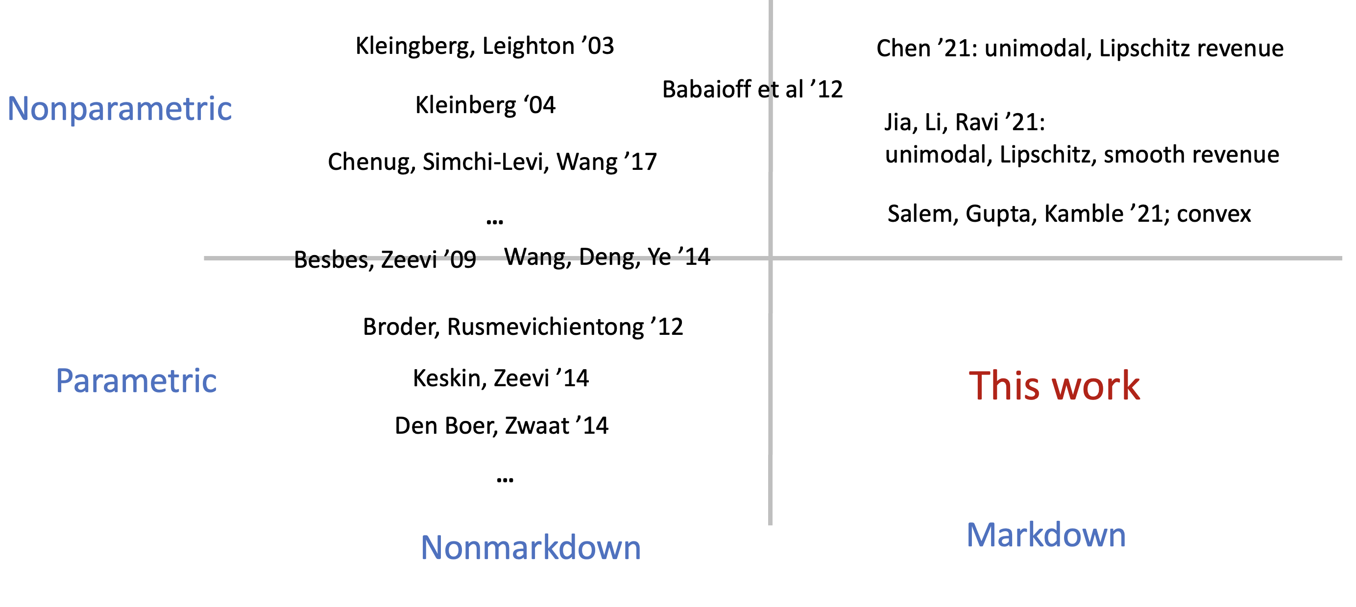
Figure 1: Landscape of dynamic pricing with unknown demand model. Papers that fit into two quadrants (e.g., Besbes and Zeevi 2009, which involved both parametric and nonparametric models) are placed on the boundary.

Recently there is an emerging line of work on bandits with monotonicity constraint. Chen (2021) and Jia et al. (2021) recently independently considered the dynamic pricing problem with monotonicity constraint under unknown demand function, and proved nearly-optimal $n^{3/4}$ regret bound assuming the reward function is Lipschitz and unimodal. Moreover, they also showed that these assumptions are indeed minimal, in the sense that no markdown policy achieves $o(T)$ regret without any one of these two assumptions. Motivated by fairness constraints, Gupta and Kamble (2019) and Salem et al. (2021) considered a general online convex optimization problem where the action sequence is required to be monotone.

Other constraints on the arm sequence motivated by practical problems are also considered in the literature. For example, motivated by the concern that customers are hostile to frequent price changes (see e.g. Dholakia (2015)), Cheung et al. (2017), Perakis and Singhvi (2019) and Simchi-Levi and Xu (2019) considered pricing policies with a given budget in the number of price changes . Motivated by clinical trials, Garivier et al. (2017) studied the best arm identification problem when the reward of the arms are monotone and the goal is to identify the arm closest to a threshold.

2 Formulation and Basic Assumptions

Given a discrete time horizon of $n$ rounds. In each round $t\in[n]:=\{1,\dots,n\}$, the seller selects a price $X_{t}\in[p_{\min},p_{\max}]$ and receives a (random) demand $D_{t}$ satisfying $\mathbb{E}[D_{t}]=d(X_{t})$ where $d:[p_{\min},p_{\max}]\rightarrow[0,1]$ is called the demand function. To reduce clutter, we assume that $p_{\min}=0$ and $p_{\max}=1$. The seller then chooses the next price based on the observations so far. This decision-making procedure can be formalized as a policy.

Definition 2.1 (Markdown policy)

For each $t\in[n]$, let $\mathcal{F}_{t}=\sigma(X_{1},D_{1},\cdots,X_{t-1},D_{t-1})$ and define the filtration $\mathcal{F}=(\mathcal{F}_{t})_{t\in[n]}$. A policy is an $\mathcal{F}$-predictable stochastic process $X=(X_{t})_{t\in[n]}$ with $X_{t}\in[0,1]$ almost surely (a.s.) for all $t\in[n]$. Furthermore, $X$ is a markdown policy if $X_{t-1}\geq X_{t}$ a.s. for each $t=2,\dots,n$.

We assume that there is an unlimited supply. Thus, when observing the demand $D_{t}$, the seller can fulfill all $D_{t}$ units and thereby receive a revenue of $R_{t}=D_{t}\cdot X_{t}$. It is sometimes convenient to work with the revenue function $r(x):=d(x)\cdot x$. One can easily verify that $\mathbb{E}[R_{t}|\mathcal{F}_{t-1}]=r(X_{t})$. The seller aims to maximize the total expected revenue $R:=\sum_{t=1}^{n}R_{t}$.

If the true demand function is known, the optimal policy is to always select the revenue-maximizing price, formally given below.

[Unique optimal price] We assume that the revenue functions $r$ has a unique maximum $p^{*}(r)$.

The uniqueness assumption is adopted for the sake of simplicity of analysis and is not essential. It is quite common in the literature, see, e.g., Assumption 1(b) of Broder and Rusmevichientong 2012 and Section 2 of den Boer and Zwart 2013.

When the demand function $d$ is unknown, we measure the performance of a policy by its loss due to not knowing $d$.

Definition 2.2 (Regret)

The regret of a policy $X=(X_{t})$ for demand function $d$ is

$$\mathrm{Reg}(X,d):=n\cdot\max_{p\in[0,1]}\{p\cdot d(p)\}-\mathbb{E}\left[\sum_{t=1}^{n}X_{t}\cdot d(X_{t})\right].$$

The regret of relative to a family $\mathcal{F}$ of demand functions is

$$\mathrm{Reg}(X,\mathcal{F}):=\sup_{d\in\mathcal{F}}\left\{\mathrm{Reg}(X,d)\right\}.$$

We first introduce a standard assumption (see, e.g., Lemma 3.11 in Kleinberg and Leighton 2003 and Corollary 2.4 in Broder and Rusmevichientong 2012) that the derivative of the revenue function vanishes at an optimal price.

[First-order optimality] The revenue function $r:[0,1]\rightarrow[0,1]$ is differentiable and $r^{\prime}(p^{*}(r))=0$.

As a standard assumption in the literature of MAB, in order to apply concentration bounds, we assume that the random rewards have light tail.

Definition 2.3 (Subgaussian Random Variable)

The subgaussian norm of a random variable $X$ is $\|X\|_{\rm sg}:=\inf\{c>0:\mathbb{E}[e^{X^{2}/c^{2}}]\leq 2\}.$ We say $X$ is subgaussian if $\|X\|_{\rm sg}<\infty$.

[Subgaussian noise] There exists a constant $c_{sg}>0$ such that the random demand $D$ at any price satisfies $\|D\|_{\rm sg}\leq c_{sg}$.

We clarify some notation before ending this section. Throughout, we will prioritize the use of capital letters for random variables and sets. We will use boldface font to denote vectors. The notation $\tilde{O}$ means that we ignore the $O(\log n)$ terms.

3 Crossing Number

We characterize the complexity of a family of demand models by introducing the crossing number. The formal definition of the crossing number may be slightly technical. We first illustrate the ideas using linear demand functions, and define the crossing number informally at the end of Section 3.1. Readers may choose to skip the remainder of this section during initial reading without affecting their understanding of the rest of the paper.

3.1 An illustrative example: linear demand

Given $\theta_{1},\theta_{2}>0$, consider the demand function

$$d(x;\theta)=\frac{1}{2}+\theta_{1}-\theta_{2}x\quad\text{for}\quad x\in\left[\frac{1}{2},1\right]$$

and consider the family $\mathcal{F}=\left\{d(x;\theta):\theta_{1},\theta_{2}\in\left[\frac{1}{2},1\right]\right\}$. Here is a natural markdown policy. Choose two exploration prices $p_{1},p_{2}$ close to $1$, and select each of them a number of times. Denote by $\bar{D}_{1},\bar{D}_{2}$ the corresponding empirical mean demands. Let $\hat{\theta}\in^{2}$ be the unique vector that satisfies $d(p_{i};\hat{\theta})=\bar{D}_{i}$ for $i=1,2$. Select the optimal price of $d(\cdot;\hat{\theta})$ in the remaining rounds.

We observe two key properties the above parameterized family. First, any two curves in the family intersects at most once. Consequently, the true demand function can be identified using only two prices, assuming that there was no noise in the realized demands. Second, the parameterization is robust: Suppose each $\bar{D}_{i}$ deviates from the mean demand $d(p_{i};\theta)$ by at most $\delta$, then the estimation error in $\theta$ is $O(\delta/|p_{1}-p_{2}|)$. In other words, the estimation error is (at most) linear in $\delta$ and the reciprocal of the “dispersion” of the exploration prices. As we will formally define shortly, any parameterized family with the above two properties is said to have crossing number $1$.

In broader terms, informally, a parameterized family has a crossing number $k$, if (i) any two curves intersect at most $k$ times and (ii) there exists a robust parametrization. Specifically, (ii) means that for any set of $k$ prices spaced at a distance of $h$ from each other, an $O(\delta)$ error in the estimated demands leads to an estimation error in the parameters of $O(\delta h^{-k})$. Under this definition, the family of degree $k$ polynomials has a crossing number $k$, under mild assumptions.

We formalize the notion of the crossing number by formally defining two concepts: the identifiability of a family (in Section 3.2) and the robustness of a parametrization (in Section 3.3).

3.2 Identifiability of a Family

Consider linear demand. Suppose $c\in(0,1)$ is an unknown constant and the demand function is $d(p;c)=1+cp$ for $p\in[0,1]$. Then, we can learn the demand function by selecting just one price. On the contrary, consider $d(p;a,b)=a-bp$ where both $a,b$ are unknown. Then, we need to select (at least) two distinct prices. Consequently, we face the following dilemma, caused by the monotonicity constraint. Suppose these two exploration prices $p<p^{\prime}$ are close by. Then, a substantial sample size is needed for reliable estimation, which leads to a high regret. On the other hand, if $p,p^{\prime}$ are far apart, then we face an overshooting risk: If the optimal price $p^{*}$ is close to $p^{\prime}$, a high regret is incurred in the remaining rounds, since we can not increase the price.

The above discussion suggests that the complexity of a family depends on the number of prices required to identify a demand function.

Definition 3.1 (Profile Mapping)

Consider a set $\mathcal{F}$ of real-valued functions defined on $[0,1]$. For any ${\bf p}=(p_{0},p_{1},\dots,p_{k})\in[0,1]^{k+1}$, the profile mapping is defined as

$$\Phi_{\bf p}:\mathcal{F} \rightarrow^{k+1},$$

$$d \mapsto\left(d(p_{0}),d(p_{1}),\dots,d(p_{k})\right).$$

We refer to $\Phi_{\bf p}(d)$ as the $\bf p$-profile of a function $d$. A family of functions is $k$-identifiable if any two functions have distinct ${\bf p}$-profile for any ${\bf p}\in[0,1]^{k+1}$. Geometrically, this means that the graphs of any two functions (i.e., “curves”) intersect at most $k$ times.

Definition 3.2 (Identifiability)

A family $\mathcal{F}$ of functions defined on $[0,1]$ is $k$-identifiable, if for any distinct prices ${\bf p}=(p_{0},p_{1},\dots,p_{k})\in[0,1]^{k+1}$, the profile mapping $\Phi_{\bf p}$ is injective, i.e., for any distinct $f,\tilde{f}\in\cal F$, we have

$$\Phi_{\bf p}(f)\neq\Phi_{\bf p}(\tilde{f}).$$

For example, the family of all degree $k$ polynomials is $k$-identifiable. We will soon use the following fact: If a family is $k$-identifiable, then for any distinct $p_{0},p_{1},\dots,p_{k}$, the profile mapping admits an inverse $\Phi_{\bf p}^{-1}:\mathcal{R}_{p}\rightarrow\mathcal{F}$ where $\mathcal{R}_{p}$ is the range of the mapping $\Phi_{\bf p}$.

3.3 Robust Parametrization

Apart from the identifiablity, we also require the family to admit a well-behaved representation, called a robust parametrization. To formalize this concept, we first define a parametrization.

Definition 3.3 (Parametrization)

Let $k\geq 1$ be an integer and $\Theta\subseteq^{k}$. An order-$k$ parametrization for a family $\mathcal{F}$ of functions is any one-to-one mapping from a set $\Theta$ to $\mathcal{F}$. Moreover, each $\theta\in\Theta$ is called a parameter.

We use $d(p;\theta)$ to denote the function in $\cal F$ that parameter $\theta$ corresponds to. For example, for $d(p;\theta_{1},\theta_{2})=\theta_{1}-\theta_{2}p$ is a parametrization of the family of linear functions. As a standard assumption (see, e.g., page 3 of Broder and Rusmevichientong (2012)), we assume that $\Theta$ is compact. [Compact Domain] The domain $\Theta$ of the parametrization is compact.

This assumption leads to several favorable properties. For example, the functions in $\mathcal{F}$ are bounded, so we lose no generality by scaling the range of those functions to $[0,1]$.

[Smoothness] The function $d:[0,1]\times\Theta\rightarrow$ is twice continuously differentiable. Consequently, there exist constants $c^{(j)}>0$, $j=0,1,2$, such that $|d^{(j)}(p,\theta)|\leq c^{(j)}$ for any $(p,\theta)\in[0,1]\times\Theta$.

By abuse of notation, we view the optimal price mapping $p^{*}$ as defined on $\Theta$ rather than on $\cal F$. For example, for $d(p;\theta_{1},\theta_{2})=\theta_{1}-\theta_{2}p$, one can verify that $p^{*}=\frac{\theta_{1}}{2\theta_{2}}$. The next assumption allows us to propagate the estimation error in $\theta$ to that of $p^{*}(\theta)$.

[Lipschitz Optimal Price Mapping] The optimal price mapping $p^{*}:\Theta\rightarrow[0,1]$ is $c^{*}$-Lipschitz for some constant $c^{*}>0$.

This assumption has appeared in the previous literature on parametric demand learning; see, e.g., Assumption 1(c) of Broder and Rusmevichientong 2012. Moreover, it is satisfied by many basic demand functions such as linear, exponential and logit functions. For instance, let $d(p;c)=1-cp$ where $p,c\in[0,1]$, then $p^{*}(c)=\min\{\frac{1}{2c},1\}$, which is $1$-Lipschitz.

The final ingredient for robust parametrization is motivated by a nice property of the natural parametrization $D(p;\theta)=\sum_{j=0}^{k}\theta_{j}p^{j}$ for polynomials. Consider any distinct $p_{0},p_{1},\dots,p_{k}$, and real numbers $y_{0},y_{1},\dots,y_{d}$ representing the mean reward at each $p_{i}$. We can uniquely determine a degree-$k$ polynomial by solving the linear equation

$$V_{\bf p}{\bf\theta}=y,\quad\text{where}\quad{\bf\theta}=(\theta_{0},\theta_{1},\dots,\theta_{k})^{T},\quad{\bf y}=(y_{0},y_{1},\dots,y_{k})^{T}$$

and

$$V_{\bf p}:=V(p_{0},\dots,p_{k})=\begin{bmatrix}&1&p_{0}&p_{0}^{2}&\cdots&p_{0}^{k}\\ &1&p_{1}&p_{1}^{2}&\cdots&p_{1}^{k}\\ &&&\vdots&&\\ &1&p_{k}&p_{k}^{2}&\cdots&p_{k}^{k}\\ \end{bmatrix}$$

is the Vandermonde matrix. One can easily verify that $V_{\bf p}$ is invertible if and only if $p_{i}$’s are distinct, in which case we have

$$\theta=V_{\bf p}^{-1}{\bf y}.$$

Next we consider the impact of a perturbation on $\bf y$, in terms of the following dispersion parameter.

Definition 3.4 (Dispersion of exploration prices)

For any ${\bf p}=(p_{0},\dots,p_{k})\in[0,1]^{k+1}$, we define the dispersion $h({\bf p}):=\min_{i\neq j}|p_{i}-p_{j}|.$

To motivate the general definition of robustness, we first consider a result specific to polynomials. Recall that $\mathcal{R}_{\bf p}$ is the range of the profile mapping $\bf\Phi_{p}$.

Proposition 3.5 (Robust Parametrization for Polynomials)

There are constants $c_{1},c_{2}>0$ such that for any ${\bf p}\in[0,1]^{k+1}$ with $0<h({\bf p})\leq c_{1}$, and ${\bf y,\hat{y}}\in\mathcal{R}_{\bf p}$ with $\|{\bf y}-{\bf\hat{y}}\|_{1}\leq c_{1}$, it holds that

$$\|V^{-1}_{\bf p}{\bf y}-V^{-1}_{\bf p}{\bf\hat{y}}\|_{1}\leq c_{2}\cdot\|{\bf y}-{\bf\hat{y}}\|_{1}\cdot h({\bf p})^{-k}.$$ (1)

More concretely, let $d(p;\theta)$ be the true demand function, then ${\bf y}=V_{\bf p}\theta$ represents the mean demands at the prices in $\bf p$. Suppose we observe empirical mean demands ${\bf\hat{Y}}=(\hat{Y}_{0},\hat{Y}_{1},\dots,\hat{Y}_{k})$ at these prices, then we have a reasonable estimation $\hat{\theta}=V^{-1}_{\bf p}\bf\hat{Y}$. Our Proposition 3.5 can then be viewed as an upper bound on the estimation error $\|\theta-\hat{\theta}\|_{1}$ in $h(\bf p)$ and $\|\bf y-\bf\hat{Y}\|_{1}$.

In order to achieve sublinear regret, we need to ensure that $h({\bf p})=o(1)$ as $n\rightarrow\infty$. Moreover, the rate of this convergence crucially affects our regret bounds. Proposition 3.5 establishes a nice property for polynomials, that the estimation error scales as $h^{-k}$ when $h\rightarrow 0^{+}$. We introduce robust parametrization by generalizing this property beyond polynomials. We say an order-$k$ parametrization is robust if the bound in Proposition 3.5 holds.

Definition 3.6 (Robust Parametrization)

An order-$k$ parametrization $\theta:\Theta\rightarrow\mathcal{F}$ is robust, if
(1) it satisfies Assumptions 3.3, 3.3 and 3.3, and
(2) there exists $c_{1},c_{2}>0$ such that for any ${\bf p}\in[0,1]^{k+1}$ with $0<h({\bf p})\leq c_{1}$ and any ${\bf y,y^{\prime}}\in\mathcal{R}_{\bf p}$ with $\|{\bf y}-{\bf y^{\prime}}\|_{1}\leq c_{1}$, we have

$$\|\Phi^{-1}_{\bf p}({\bf y})-\Phi^{-1}_{\bf p}({\bf y^{\prime}})\|_{1}\leq c_{2}\cdot\|{\bf y}-{\bf y^{\prime}}\|_{1}\cdot h({\bf p})^{-k}.$$ (2)

In particular, when $k=0$, this inequality simply means that ${\bf\Phi_{p}^{-1}}$ is $c_{2}$-Lipschitz.

3.4 Crossing Number of a Family

Now we are ready to define the crossing number.

Definition 3.7 (Crossing number)

The crossing number of a family $\mathcal{F}$ of functions, denoted $\kappa(\mathcal{F})$, is the minimum integer $k\geq 0$ such that $\mathcal{F}$ (i) is $k$-identifiable and (ii) admits a robust order-$k$ parametrization. If no finite $k$ satisfies the above, then $\kappa(\mathcal{F}):=\infty$. A family with a crossing number $k$ is also called $k$-crossing.

We illustrate our definition by considering the crossing numbers of some basic families. As one important example, our definition of the $0$-crossing family is equivalent to the separable family defined in Section 4 of Broder and Rusmevichientong 2012. Here, we provide a few concrete examples, with proofs deferred to Appendix 6.

Proposition 3.8 ($0$-crossing Families)

The following families are $0$-crossing:
(1) The single-parameter linear family $\mathcal{F}_{1}=\{d_{a}(x):a\in\left[\frac{1}{2},1\right]\}$ where $d_{a}(x)=1-ax$ for $x\in[\frac{1}{2},1]$,
(2) The exponential family $\mathcal{F}_{2}=\left\{d_{a}(x):a\in\left[\frac{1}{2},\frac{3}{4}\right]\right\}$ where $d_{a}(x)=e^{1-ax}$ for $x\in[\frac{1}{2},1]$, and
(3) The logit family $\mathcal{F}_{3}=\left\{D_{a}(x):a\in\left[\frac{1}{2},1\right]\right\}$ where $d_{a}(x)=\frac{e^{1-ax}}{1+e^{1-ax}}$ for $x\in\left[\frac{1}{2},1\right]$.

Proposition 3.9 (Degree-$k$ polynomial family is $k$-crossing)

Define $d(x;\theta)=\sum_{j=0}^{k}\theta_{j}x^{j}$. Suppose $\mathcal{F}=\{d(x;\theta):\theta\in\Theta\}$ satisfies Assumptions 3.3, 3.3 and 3.3, then $\kappa(\mathcal{F})=k$.

We defer the proof to Appendix 6. Finally, note that if a family is not $k$-identifiable for any $k$, then $\kappa(\cal F)=\infty$. One example is the Lipschitz family. In fact, for any $k<\infty$ distinct prices, there exist multiple (more precisely, infinitely many) Lipschitz functions having the same values on these $k$ prices.

Proposition 3.10 (Lipschitz family is $\infty$-crossing)

Let $\mathcal{F}$ be the family of $1$-Lipschitz functions on $[0,1]$, then $\kappa(\mathcal{F})=\infty$.

3.5 Sensitivity

Finally, we introduce the notion of sensitivity to refine our categorization of families. For intuition, consider the Taylor expansion of a revenue function $r(p)$ around $p^{*}$:

$$r(p)=r(p^{*})+0+\frac{1}{2!}r^{\prime\prime}(p^{*})(p-p^{*})^{2}+\frac{1}{3!}r^{(3)}(p^{*})(p-p^{*})^{3}+\cdots,$$

where the “$0$” follows from the first-order optimality condition (Assumption 2). Suppose the first nonzero derivative is $r^{(j)}(p^{*})$. Then, the higher $j$, the less sensitive the revenue is to the estimation error in $p^{*}$. We capture this aspect in the following notion of sensitivity.

Definition 3.11 (Sensitivity)

A revenue function $r$ is $s$-sensitive if it is $(s+1)$-times continuously differentiable with $r^{(1)}\left(p^{*}(r)\right)=\cdots=r^{(s-1)}\left(p^{*}(r)\right)=0$ and $r^{(s)}\left(p^{*}(r)\right)<0$. A family $\mathcal{F}$ of reward functions is called $s$-sensitive if
(a) every $r\in\mathcal{F}$ is $s$-sensitive,
(b) it admits a parametrization $r(p;\theta)$ satisfying Assumptions 3.3 to 3.3,
(c) there is a constant $c_{6}>0$ such that $r^{(s)}\left(p^{*}(r)\right)\leq-c_{6}<0$ for any $r\in\mathcal{F}$, and
(d) for each $0\leq j\leq s$, there exists a constant $c^{(j)}$ such that $|r^{(j)}(x;\theta)|\leq c^{(j)}$, $\forall x\in[0,1]$ and $\theta\in\Theta$.

For example, let $s\geq 3$ and $r(x;\theta)=\theta-|\frac{1}{2}-x|^{s}$ for $x\in[0,1]$ and any $\theta\in$, then $\{r(x;\theta):\theta\in[\frac{1}{2},1]\}$ is an $s$-sensitive family. Note that by Taylor’s Theorem, we have

$$|r(p^{*}+\varepsilon)-r(p^{*})|=O(\varepsilon^{s}).$$

Consequently, if a policy undershoots or overshoots the optimal price by $\varepsilon$, then the regret per round is $O(\varepsilon^{s})$, which is lower than the per-round regret $O(\varepsilon^{2})$ in the basic case. In each of the next three sections, we will first present the regret bounds for the basic case $s=2$, and then characterize how this bound improves as $s$ increases.

4 Zero-crossing Family

Broder and Rusmevichientong (2012) considered the an important special case of the demand learning problem under the so-called well-separated assumption without the monotonicity constraint; see their Section 4. Loosely, this definition states that at any price, any two demand functions are distinguishable. This definition closely resembles our definition of a $0$-crossing, with a slight and non-essential difference, wherein they assumed that the Fisher information is bounded away from $0$, while we assume that the inverse profile mapping is well-conditioned. Despite this slight technical discrepancy, it is straightforward to verify that their analysis for well-separated families remains valid for our $0$-crossing families.

Specifically, they proposed the following MLE-greedy policy: In each round, we estimate the true parameter using the maximum likelihood estimator (MLE), and select the optimal price of the estimated demand function. In their Theorem 4.8, they showed that this policy has regret $O(\log n)$. This follows from the basic fact that the mean squared error (MSE) of MLE with a sample size $t$ is $\Theta(t^{-1})$, which implies that the expected total regret is $\sum_{t=1}^{n}O(t^{-1})=O(\log n)$.

They also showed that this bound is minimax optimal; see their Theorem 4.5. More precisely, they constructed a family of linear demand functions and showed that any policy suffers $\Omega(\log n)$ regret. This family can be easily verified to have a crossing number of $0$; see our Proposition 3.8. To facilitate a more direct comparison of their results with ours, let us express the above bounds using our terminology.

Theorem 4.1 (Regret without monotonicity, $k=0$)

For any $0$-crossing family $\mathcal{F}$, we have ${\rm Reg}(\textrm{MLE-greedy},\mathcal{F})=O(\log n).$ Moreover, there exists a $0$-crossing family $\mathcal{F}$ such that for any policy $X$, we have ${\rm Reg}(X,\mathcal{F})=\Omega(\log n).$

Algorithm 1 Cautious Myopic (CM) Policy

1:Input: a family $\mathcal{F}$ of demand functions and time horizon $n$.

2:$P_{1}\leftarrow 1$ $\triangleright$ Initialization

3:for $j=1,\dots,m$ do

4:     for $t=t^{(j-1)}+1,\dots,t^{(j-1)}+t_{j}$ do$\triangleright$ Select price $P_{j}$ in the next $t_{j}$ rounds

5:         $X_{t}\leftarrow P_{j}$

6:         Observe demand $D_{t}$      

7:     $\bar{D}_{j}=\frac{1}{t_{j}}\sum_{\tau=1}^{t_{j}}D_{t^{(j-1)}+\tau}$$\triangleright$ Empirical mean demand in phase $j$

8:     $\hat{\theta}_{j}\leftarrow\Phi^{-1}_{P_{j}}(\bar{D}_{j})$ $\triangleright$ Estimate parameter

9:     $w_{j}\leftarrow 4c_{2}\cdot c_{\rm sg}\sqrt{\frac{\log n}{t_{j}}}$$\triangleright$ Width of the confidence interval

10:     $\tilde{P}_{j+1}\leftarrow\max\left\{p^{*}(\theta):|\theta-\hat{\theta}_{j}|\leq w_{j}\right\}$ $\triangleright$ Conservative estimation of the optimal price

11:     $P_{j+1}\leftarrow\min\left\{\tilde{P}_{j+1},P_{j}\right\}$ $\triangleright$ Ensure monotonicity

Apparently, the price sequence in the MLE-Greedy policy may not be monotone - the number of price increases can be $\Omega(n)$. We propose the following markdown policy, dubbed the Cautious Myopic (CM) policy. In contrast to the famous principle of optimism under uncertainty (e.g., in UCB-type policies), our policy adopts conservatism under uncertainty. We partition the time horizon into phases where phase $j$ consists of $t_{j}=\lceil 9^{j}\log n\rceil$ rounds. It can be verified that the total number of phases is $m=O(\log n-\log\log n)$. In each phase, the policy builds a confidence interval $I_{j}$ for the true parameter using the observations from (only) this phase and sets the price for phase $j+1$ to be the largest optimal price of any “surviving” parameter $\theta\in I_{j}$. We formally state this policy in Algorithm 1.

We show that the CM policy has regret $O(\log^{2}n)$. Denote $t^{(j)}:=\sum^{j}_{k=0}t_{k}$ and $t^{(0)}=0$.

Theorem 4.2 (Upper bound, $k=0$)

For any $0$-crossing family $\mathcal{F}$, we have

$$\mathrm{Reg}(\mathrm{CM},\mathcal{F})=O(\log^{2}n).$$

It is worth noting that this bound is asymptotically higher than the $O(\log n)$ upper bound for unconstrained pricing, as stated in Theorem 4.1. This is because the CM policy purposely makes conservative choices of prices to avoid overshooting. A natural question then is: Can we achieve $o(\log^{2}n)$ regret by behaving less conservatively? We answer this question negatively, and provide a separation between markdown and unconstrained pricing for crossing number $0$.

Theorem 4.3 (Lower bound, $k=0$)

There exists a $0$-crossing family $\cal F$ of demand functions such that for any policy $X=(X_{t})_{t\in[n]}$, we have

$$\mathrm{Reg}(X,\mathcal{F})\geq\Omega\left(\log^{2}n\right).$$

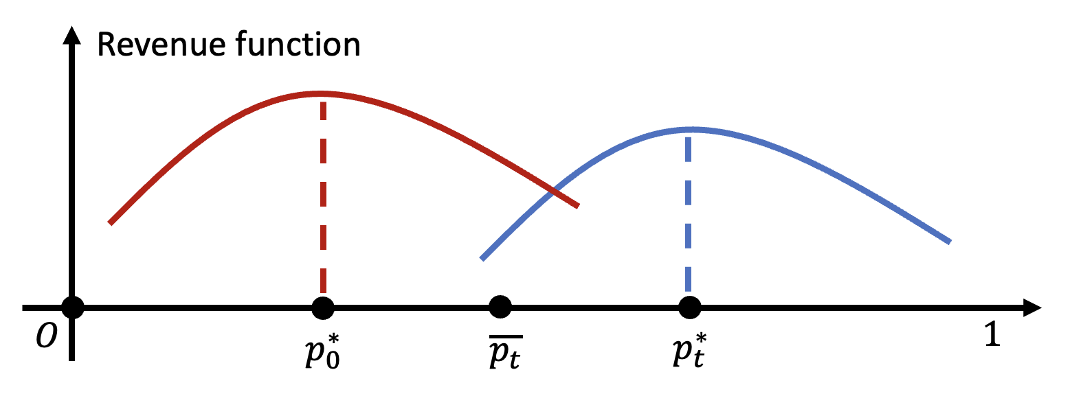
Figure 2: Illustration of the lower bound proof for $0$-crossing demand family. The red and blue curves correspond to the revenue functions of $d_{0}(\cdot)$ and $d_{t}(\cdot)$ for a fixed round $t$. Due to the monotonicity constraint, to avoid high regret for the blue curve, we need the event $X_{t}>\bar{p}_{t}$ to occur w.h.p. This in turn implies that $X_{t}>\bar{p}_{t}$ also occurs with $\Omega(1)$ Phys. Rev. B for the red curve, leading to a high regret in this round.

We describe the proof at a high level and defer the details to Appendix LABEL:apdx:lb_d=1. Fix a round $t=O(\sqrt{n})$ and a linear demand function $d_{0}(x;\theta)=1-\theta x$ whose optimal price satisfies $p^{*}_{0}\in(\frac{1}{2},1)$. We bound the expected regret in round $t$ as follows. Choose $\delta_{t}=O(\sqrt{t^{-1}\log n})$ and construct another demand function $d_{t}(x)=1-\theta_{t}x$ whose optimal price $p^{*}_{t}$ satisfies $p^{*}_{t}\geq p^{*}_{0}+\delta_{t}$; see Figure 2.

Consider the midpoint $\bar{p}=\bar{p}_{t}:=(p^{*}_{t}+p^{*}_{0})/2$. To avoid a high regret for $d_{t}(\cdot)$, the price $X_{t}$ at time $t$ must be greater than $\bar{p}$ with high Phys. Rev. B (w.h.p.). In fact, due to the monotonicity constraint, once the price is lower than $\bar{p}$, we can not increase it back to the neighborhood of $p^{*}_{t}$, which leads to an $\Omega(\delta_{t}^{2})$ regret in all future rounds. More precisely, if $X_{t}<\bar{p}_{t}$ occurs with Phys. Rev. B $\Omega(n^{-1/2}\log n)$, then the total regret in the remaining $n-t$ rounds is

$$\Omega\left(\frac{\log n}{\sqrt{n}}\right)\cdot\Omega(\delta_{t}^{2})\cdot(n-t)=\Omega\left(\frac{\log n}{\sqrt{n}}\cdot\frac{\log n}{t}\cdot n\right)=\Omega\left(\log^{2}n\right),$$

where we used the assumption that $t=O(\sqrt{n})$.

Therefore, to achieve low regret, the policy must exercise exceptional caution to go below $\bar{p}_{t}$. However, this in turn leads to a high regret under $d_{0}$. Using a result on the sample complexity of adaptive hypothesis testing policies due to Wald and Wolfowitz (1948), we can show that $X_{t}>\bar{p}_{t}$ occurs with Phys. Rev. B $\Omega(1)$ when $d_{0}$ is the true demand model. Furthermore, when this event occurs, we incur a regret of $\Omega(\delta_{t}^{2})$. Note that this argument holds for any $t=1,\dots,\sqrt{n}$, so we can lower bound the total regret as

$$\sum_{t=1}^{O(\sqrt{n})}\Omega(\delta^{2}_{t})\cdot\Omega(1)=\Omega\left(\sum_{t=1}^{O(\sqrt{n})}\frac{\log n}{t}\right)=\Omega\left(\log^{2}n\right).$$

We end this section with a natural generalization. Recall that any family satisfying our regularity assumptions (Assumption 3.3) has sensitivity $s\geq 2$. Interestingly, we show that if $s>2$, the upper bound can be improved to $O(\log n)$, which matches the optimal regret bound without the monotonicity constraint.

Theorem 4.4 (Zero-crossing Upper Bound, higher sensitivity)

Let $s>2$ and $\mathcal{F}$ be a $0$-crossing, $s$-sensitive family of demand functions. Then,

$$\mathrm{Reg}(\mathrm{CM},\mathcal{F})=O(\log n).$$

So far we have characterized the minimax regret for $0$-crossing families. Next, we study the finite-crossing families and analyze a different conservatism-based policy.

5 Finite-crossing Family

For the crossing number $k\geq 1$, the seller needs $k+1$ distinct exploration prices, as opposed to just one for $k=0$ in the last section. However, this brings about additional regret, since the optimal price can lie between these exploration prices. A policy faces the following trade-off. Suppose we select exploration prices $P_{0}>P_{1}>\dots>P_{k}$ sequentially, each sufficiently many times. If these prices are spread out, the policy may learn the parameter efficiently. However, there is potentially incurs a high regret for overshooting, which could happen if the optimal price lies close to $P_{0}$. On the other extreme, if these prices are concentrated, we need a large sample size for a good estimate, which also leads to a high regret.

5.1 The Iterative Cautious Myopic Policy

We handle the above dilemma by the following the Iterative Cautious Myopic (ICM) policy, formally stated in Algorithm 2. This policy is specified by three types of policy parameters: (i) the maximum number $m$ of exploration phases, (ii) the distance $h$ between neighboring exploration prices, and (iii) the numbers $n_{j}$ of times we select each exploration price in phase $j=1,\dots,m$. We emphasize that $h$ is the same for all phases, but $n_{j}$ can vary between phases $j$.

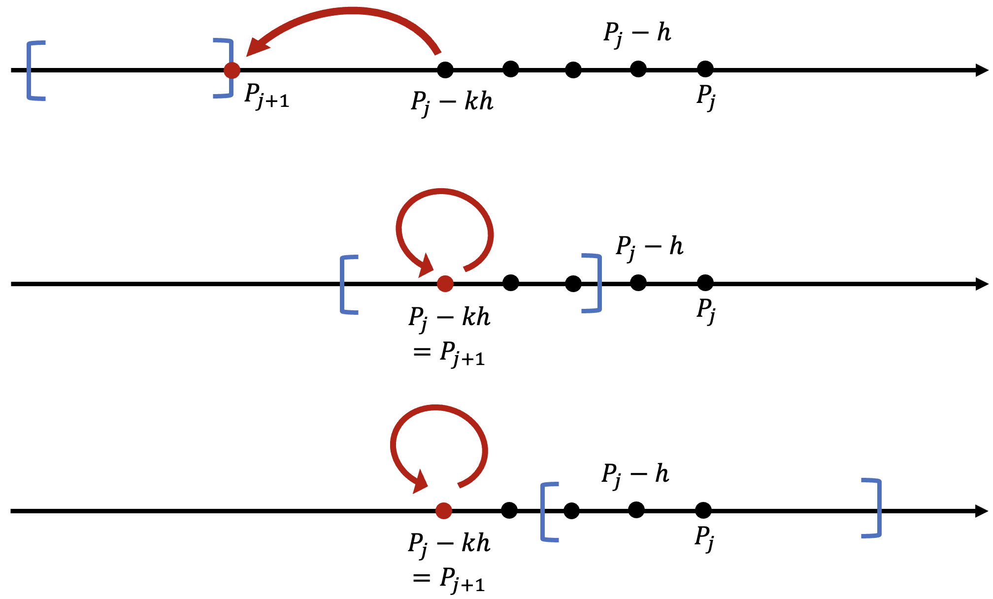
Figure 3: The three subfigures correspond to the good, dangerous and bad events respectively. The blue interval represents the confidence interval $[L_{j},U_{j}]$, obtained using observations from the exploration prices $P_{j},P_{j}-h,\dots,P_{j}-kh$. The red arrow indicates the starting exploration price in the next phase, i.e., $P_{j+1}$.

The policy starts at the price $P_{0}=1$. In phase $j\in[m]$, the policy selects prices $P_{j},P_{j}-h,\cdots,P_{j}-kh$ each for $n_{j}$ times. Based on the observed demands at these prices, the policy computes a confidence interval $[L_{j},U_{j}]$ for the optimal price. To determine the starting price $P_{j+1}$ in the next phase, we consider the relation between the confidence interval $[L_{j},U_{j}]$ and the current price, i.e., $P_{j}-kh$. Consider the following three cases, as illustrated in Figure 3.
1. Good event. If $P_{j}-kh>U_{j}$, then we get closer to the optimal price by setting $P_{j+1}\leftarrow U_{j}$.
2. Dangerous event. If $L_{j}\leq P_{j}-kh\leq U_{j}$, i.e., the current price is already inside the confidence interval. To avoid overshooting the optimal price, we behave conservatively by choosing $P_{j+1}$ to be the highest price allowed, i.e., $P_{j+1}\leftarrow P_{j}-kh.$
3. Overshooting event. If $P_{j}-kh<L_{j}$, then w.h.p. we have overshot, i.e., the current price is lower than $p^{*}$, so we immediately terminate the exploration phase and select the current price in all remaining rounds.

1:Input:

2: $\mathcal{F}:$ a family of demand functions,

3: $m$: number of phases,

4: $n_{1},\dots,n_{m}$: length of each phase,

5: $n:$ length of the time horizon.

6:Initialization: $P_{1}\leftarrow 1,L_{0}\leftarrow 0,U_{0}\leftarrow 1$

7:for $j=1,2,\dots,m$ do$\triangleright$ Phase $j$

8:     for $i=0,1,\dots,k$ do$\triangleright$ Exploration price $i$

9:         Select price $P_{j}-ih$ for $n_{j}$ times in a row and observe demands $D_{1},\dots,D_{n_{j}}$

10:         $\bar{D}_{\ell}\leftarrow\frac{1}{n_{j}}\sum_{i=1}^{n_{j}}D_{i}$$\triangleright$ Empirical mean demand at $P_{j}-ih$      

11:     $\hat{\theta}\leftarrow\Phi^{-1}_{P_{j},\dots,P_{j}-kh}\left(\bar{D}_{0},\dots,\bar{D}_{k}\right)$ $\triangleright$ Estimate the parameter

12:     $w_{j}\leftarrow 2h^{-k}c_{2}\cdot c_{\rm sg}\sqrt{\frac{k\log n}{n_{j}}}$ $\triangleright$ Width of confidence interval

13:     $L_{j}\leftarrow\min\{p^{*}(\theta):\|\theta-p^{*}(\hat{\theta})\|_{2}\leq w_{j}\}$ $\triangleright$ Lower confidence bound

14:     $U_{j}\leftarrow\max\{p^{*}(\theta):\|\theta-p^{*}(\hat{\theta})\|_{2}\leq w_{j}\}$ $\triangleright$ Upper confidence bound

15:     if $U_{j}>P_{j}-kh$ then

16:         $P_{j+1}\leftarrow U_{j}$ $\triangleright$ Good event      

17:     if $U_{j}\geq P_{j}-kh\geq L_{j}$ then

18:         $P_{j+1}\leftarrow P_{j}-kh$ $\triangleright$ Dangerous event      

19:     if $P_{j}-kh<L_{j}$ then

20:         Break$\triangleright$ Overshooting event      

21:Select the current price in every future round $\triangleright$ Exploitation

Algorithm 2 The Iterative Cautious Myopic (ICM) Policy

5.2 Regret Analysis of the ICM Policy

We first present a general upper bound on the regret of the ICM policy for arbitrary $h$ and $n_{j}$’s.

Proposition 5.1 (Upper bound, finite-crossing family)

Let $\mathcal{F}$ be a $k$-crossing, $s$-sensitive family of demand functions where $s\geq 2$. Suppose $h\in(0,1)$ and $1=:n_{0}<n_{1}<\dots<n_{m}$ where $n_{m}=o(n)$. Denote $\mathrm{ICM}=\mathrm{ICM}(n_{1},\dots,n_{m},h)$. Then,

$$\mathrm{Reg}(\mathrm{ICM},\mathcal{F}) \leq c_{s}\left(3c^{*}c_{\rm sg}k\frac{\sqrt{c_{5}k\log n}}{h^{k}}\right)^{s}\left(\sum_{j=1}^{m-1}\frac{n_{j}}{n_{j-1}^{s/2}}+\frac{n}{n_{m}^{s/2}}\right)+c_{s}\left(mkh\right)^{s}n+\frac{2mk}{n^{2}}$$ (3)

$$=\widetilde{O}\left(h^{-sk}\left(\sum_{j=1}^{m-1}\frac{n_{j}}{n_{j-1}^{s/2}}+\frac{n}{n_{m}^{s/2}}\right)+h^{s}n\right).$$

To clarify, in the above “$\tilde{O}$” notation, we view $m,k$ as small constants and suppressed them along with $\log n$ and constant terms. This is done to highlight the dependence on the most important policy parameters, such as $(n_{j})$ and $h$.

Let us sketch the proof before finding the optimal choice of $(n_{j})$. Suppose the ICM policy enters some phase $j\geq 1$ before the exploration ends (i.e., before the overshooting event occurs). Denote by ${\bf Y}\in^{\{0,1,\cdots,k\}}$ the true demand vector, i.e.,

$${\bf Y}=\left(d(P_{0};\theta),d(P_{k};\theta),\dots,d(P_{k};\theta)\right).$$

Similarly, let the vector ${\bf Y^{\prime}}\in^{\{0,1,\dots,k\}}$ denote the empirical demand observed at the exploration prices. By Hoeffding’s inequality (formally stated in Appendix 7), w.h.p. each entry of ${\bf Y^{\prime}}$ deviates from ${\bf Y}$ by $\tilde{O}(n_{j}^{-1/2})$, and hence

$$\left\|{\bf Y}-{\bf Y^{\prime}}\right\|_{1}=\tilde{O}\left(kn_{j}^{-1/2}\right).$$

Denoting the estimated parameter $\hat{\theta}$, then by eqn. (1) in the definition of robust parametrization (Definition 3.6), the estimation error is bounded as

$$\|\theta-\hat{\theta}\|_{1}=\|\Phi_{P_{0},\dots,P_{k}}^{-1}({\bf Y})-\Phi_{P_{0},\dots,P_{k}}^{-1}({\bf Y^{\prime}})\|_{1}\leq c_{2}\cdot\|{\bf Y}-{\bf Y^{\prime}}\|_{1}\cdot h^{-k}=\tilde{O}\left(kn_{j}^{-1/2}h^{-k}\right).$$

By Lipschitzness of the optimal price mapping $p^{*}(\cdot)$, the error of the estimated optimal price is also $\tilde{O}(kn_{j}^{-1/2}h^{-k})$. Finally, by the definition of sensitivity and recalling that phase $j$ consists of $(k+1)n_{j}$ rounds, we can bound the regret in this phase as

$$\tilde{O}\left(kn_{j}\cdot(kh^{-k}n_{j-1}^{-1/2})^{s}\right).$$

Similarly, setting $n_{m+1}:=\Theta(m)$, we can bound the regret in the exploitation phase as $\tilde{O}(kn\cdot(h^{-k}\cdot n_{m}^{-1/2})^{s})$.

Finally, we interpret the last term, $(mkh)^{s}n$, in eqn. (3). This term corresponds to the overshooting risk, i.e., the regret caused by going lower than the optimal price $p^{*}$. In fact, suppose the exploration phase ends due to the overshooting event in some phase $j\geq 1$, then $P_{j}-kh<L_{j}.$ By the construction of the confidence interval, we have $p^{*}\in[L_{j},U_{j}]$ w.h.p. Thus,

$$|(P_{j}-kh)-p^{*}|\leq kh+|L_{j}-U_{j}|.$$

Again, by the definition of sensitivity, the regret in exploitation phase is

$$\tilde{O}\left((kh+|L_{j}-U_{j}|)^{s}\cdot n\right).$$ (4)

Finally, by straightforward algebraic manipulation, we can merge the term $|L_{j}-U_{j}|^{s}$ into the second term in eqn. (3) and simplify eqn. (4) as $\tilde{O}((mkh)^{s}\cdot n)$.

We emphasize that this explanation is only for the purpose of high-level understanding. The formal proof involves handling numerous technical intricacies for each of the three events and is postponed to Appendix 7.

With Proposition 5.1, it is straightforward to find the (asymptotically) optimal choice of the policy parameters. In Appendix 7, we show that this can be reduced to a linear program, which can be optimized by choosing $n_{j}$’s and $h$ so that all terms in eqn. (3) have the same asymptotic order. This leads to the following regret bound.

Theorem 5.2 (Upper bound for finite crossing number)

Suppose $m=O(\log n)$. For any $s\geq 2$-sensitive, $k$-crossing family $\cal F$, there exists $n_{1}<\dots<n_{m}$ such that

$$\mathrm{Reg}(\mathrm{ICM},\mathcal{F})=\tilde{O}\left(n^{\rho(m,s,k)}\right)\quad\text{where}\quad\rho(m,s,k)=\frac{1+\left(1+\frac{s}{2}+...+(\frac{s}{2})^{m-1}\right)k}{\left(\frac{s}{2}\right)^{m}+\left(1+\frac{s}{2}+...+(\frac{s}{2})^{m-1}\right)\cdot(k+1)}.$$

In particular, if $s=2$, then for $h=n^{\frac{m}{m(k+1)+1}}$ and $n_{j}=n^{\frac{mk+j}{m(k+1)+1}}$, $j=1,\dots,m$, we have

$$\mathrm{Reg}\left(\mathrm{ICM},\mathcal{F}\right)=\tilde{O}\left(n^{\frac{k}{k+1}}\right).$$

Prior to this work, the best known regret bound for non-parametric, twice continuously differentiable family is $\tilde{O}(n^{5/7})$; see Theorem 2 in Jia et al. 2021. Our Theorem 5.2 improves the above bound to $\tilde{O}(\sqrt{n})$ for $k=1$, and to $\tilde{O}(n^{2/3})$ for $k=2$.

5.3 Lower Bound

We show a lower bound that matches the upper bound up to $O(\log n)$ factors.

Theorem 5.3 (Lower bound for finite $k\geq 1$)

For any $k\geq 2$, there exists a $k$-crossing family $\mathcal{F}$ of demand functions such that for any markdown policy $X$, we have

$$\mathrm{Reg}(X,\mathcal{F})=\Omega\left(n^{\frac{k}{k+1}}\right).$$

In our proof, for each $k\geq 1$ we construct a family of decreasing, degree-$k$ polynomials – which is also $k$-crossing – on which any policy suffers regret $\Omega(n^{k/(k+1)})$.

We conclude the section by comparing the above lower bound with the known results in the nonparametric setting. Jia et al. (2021) showed that there is a policy that achieves $\tilde{O}(n^{5/7})$ regret if the revenue function is unimodal and twice continuously differentiable. On the other hand, for $k\geq 3$, the lower bound in Theorem 5.3 is $\Omega(n^{3/4})$, which is higher than $\tilde{O}(n^{5/7})$. But this is not a contradiction, since for $k\geq 3$, the revenue functions in our lower bound proof may not be unimodal.

6 Omitted Proofs in Section 2

6.1 Proof of Propositions 3.5 and 3.9

The following definition of the matrix norm can be found in eqn (1.4) of Gautschi 1962. It can be alternatively viewed as the operator norm of the corresponding linear mapping under the $L_{1}$-norm.

Definition 6.1 (Matrix norm)

For any $A\in^{m\times m}$, define

$$\|A\|_{\rm op}:=\max_{i\in[n]}\sum_{j\in[m]}|a_{ij}|=\sup_{\|v\|_{1}\leq 1}\|Av\|_{1}.$$

By this definition, for any vector $w$, we have $\|Av\|_{1}\leq\|A\|_{\rm op}\cdot\|v\|_{1}$. Sometimes we need to consider other $L_{p}$ norms. The following basic fact will be useful.

Lemma 6.2 ($L_{p}$ norm do not differ by much)

For any $v\in^{m}$ and $p$ with $1\leq p\leq q\leq\infty$, we have

$$\|v\|_{q}\leq\|v\|p\leq m\cdot\|v\|_{q}$$

The inverse Vandermonde matrix (IMV) admits a (somewhat complicated) closed-form expression due to Gautschi (1962), which leads to the following upper bound on its matrix norm.

Theorem 6.3 (Matrix norm of the IMV)

Let $V=V(x_{1},\dots,x_{m})$ be the Vandermonde matrix  of distinct real numbers $x_{1},\dots,x_{m}$. Then,

$$\|V^{-1}\|_{\rm op}\leq\max_{i\in[m]}\prod_{j\neq i}\frac{1+|x_{j}|}{|x_{j}-x_{i}|}.$$

Let us apply this result to our problem. Recall that for any distinct prices $(p_{0},p_{1},\dots,p_{k})=:{\bf p}$, we defined $h({\bf p})=\min_{i\neq j}\{|p_{i}-p_{j}|\}$. We can bound $\|V^{-1}_{\bf p}\|_{\rm op}$ in terms of $h(\bf p)$ using Theorem 6.3.

Corollary 6.4 (Bounding the norm of the IVM using $h({\bf p})$)

For any ${\bf p}=(p_{0},p_{1},\dots,p_{k})\in[0,1]^{k+1}$ with distinct entries, it holds that

$$\|V^{-1}_{\bf p}\|_{\rm op}\leq\frac{2^{k}}{h({\bf p})^{k}}.$$

Proof 6.5

Proof. Fix any $i\in[m]$. Since $0\leq p_{j}\leq 1$ for any $j\in[n]$, we have $1+|p_{j}|\leq 2$. Therefore,

$$\prod_{j=1,j\neq i}\frac{1+|x_{j}|}{|x_{j}-x_{i}|}\leq\frac{2^{k}}{h({\bf p})^{k}}.$$

We now use the above to show that the family of degree-$k$ polynomials have crossing number $k$. Recall that $\mathcal{R}(\cdot)$ denotes the range of a mapping.

Proof of Proposition 3.5 and  3.9. Fix any ${\bf p}=(p_{0},p_{1},\cdots,p_{k})\in[0,1]^{k+1}$ with distinct entries. Then, for any $y,y^{\prime}\in\mathcal{R}(V_{\bf p})$, we have

$$\|V_{\bf p}^{-1}y^{\prime}-V_{\bf p}^{-1}y\|_{1}\leq\|V_{\bf p}^{-1}\|_{\rm op}\cdot\|y^{\prime}-y\|_{1}\leq\frac{2^{k}}{h({\bf p})^{k}}\cdot\|y^{\prime}-y\|_{1},$$

where the first inequality follows from Lemma 6.2 and the second follows from Corollary 6.4. Proposition 3.5 then follows by selecting the constant $c_{2}$ to be $2^{k}$. So far we have shown that the natural parametrization of polynomial is robust, and therefore $\kappa(\mathcal{F})\leq k$. Moreover, for any $\ell<k$, the family $F$ is not $\ell$-identifiable, since there exists a degree-$k$ polynomial with $\ell$ real roots. It follows that $\kappa(\mathcal{F})\geq k$, and therefore we obtain Proposition 3.9.

6.2 Proof of Proposition 3.8(a)

We first observe that $\mathcal{F}_{1}$ is $0$-identifiable, i.e., for any fixed $p\in[\frac{1}{2},1]$, the function $d(p;a)$ is injective in $a$. In fact, for any $a,a^{\prime}\in[\frac{1}{2},1]$, $d(p;a)=d(p;a^{\prime})$ is equivalent to $p\cdot(a-a^{\prime})=0$, which implies $a=a^{\prime}$ since $x\neq 0$.

Next, we verify that the parametrization $a\mapsto d(\cdot;a)$ is robust. This involves verifying the following conditions, as required in Definition 3.6.
(1) Lipschitz optimal price mapping. For any $a\in[\frac{1}{2},1]$, the revenue function $r(p;a)=a(1-ap)$ has a unique optimal price $p^{*}(a)=\frac{1}{2a}$, which is $2$-Lipschitz.
(2) Robust under perturbation. For any fixed price $p\in[\frac{1}{2},1]$, by the definition of profile mapping $\Phi$, we have $\Phi_{p}(a)=1-ap$. For any $y\in\mathcal{R}(\Phi_{p})$, where we recall that $\mathcal{R}(\cdot)$ denotes the range of a mapping, we have $\Phi_{p}^{-1}(y)=(1-y)/p.$ Thus, for any $y,y^{\prime}\in\mathcal{R}(\Phi_{p})$, we have

$$\left|\Phi_{p}^{-1}(y)-\Phi_{p}^{-1}(y^{\prime})\right|=\left|\frac{1-y}{p}-\frac{1-y^{\prime}}{p}\right|=\frac{|y-y^{\prime}|}{p}\leq 2\cdot|y-y^{\prime}|.$$

Therefore, the parametrization $a\mapsto D(\cdot;a)$ is robust, and therefore $\mathcal{F}_{1}$ has a crossing number $0$.

6.3 Proof of Proposition 3.8(b)

Write $d(x;a)=e^{1-ax}$. The following will be useful for (b) and (c), whose proof follows directly from the definition of identifiability.

Lemma 6.6 (Monotone link function preserves identifiablity)

Let $g:\rightarrow$ be a strictly monotone function and $\{d(x;\theta):\theta\in\Theta\}$ be a $0$-identifiable family. Then, $\{g(d(x;\theta)):\theta\in\Theta\}$ is also $0$-identifiable.

Since $\mathcal{F}_{1}$ is $0$-identifiable, and $g(z)=e^{z}$ is strictly increasing, by Lemma 6.6, $\mathcal{F}_{2}$ is also $0$-identifiable. It remains to show that $a\mapsto d(\cdot;a)$ is robust for $\mathcal{F}_{2}$, which we verify as follows.
(1) Lipschitz optimal price mapping. For any $a$, the corresponding reward function is $r(p;a)=a\cdot e^{1-ap}$. A price $p$ is then a local optimum if and only if the derivative of $r^{\prime}(p;a)=(1-ap)e^{1-ap}=0$, i.e., $x=\frac{1}{2a}$, which has just been verified to be Lipschitz in the proof for (a).
(2) Robust under perturbation. For any fixed price $p\in[\frac{1}{2},1]$, we have $\Phi_{p}(a)=e^{1-ap}$, and therefore for any $y\in\mathcal{R}(\Phi_{p})$, we have $\Phi_{p}^{-1}(y)=\frac{1-\ln y}{p}$. Thus, for any $y,y^{\prime}\in\mathcal{R}(\Phi_{p})$,

$$\left|\Phi_{p}^{-1}(y)-\Phi_{p}^{-1}(y^{\prime})\right|=\left|\frac{1-\ln y}{p}-\frac{1-\ln y^{\prime}}{p}\right|=\frac{|\ln y-\ln y^{\prime}|}{p}.$$ (5)

Finally, to bound the above, note that $e^{\frac{1}{4}}\leq e^{1-ap}\leq e^{\frac{3}{4}}$ for any $p\in\left[\frac{1}{2},1\right]$ and $a\in\left[\frac{1}{2},\frac{3}{4}\right]$, i.e.,

$$\mathcal{R}(\Phi_{p})\subseteq\left[e^{\frac{1}{4}},e^{\frac{3}{4}}\right].$$

Thus, for any $p\in[\frac{1}{2},1]$,

$$\eqref{eqn:jul30}\leq\frac{\max_{t\in\mathcal{R}(\Phi_{p})}\ln^{\prime}t}{p}\cdot\left|y-y^{\prime}\right|=2e^{-\frac{1}{4}}\cdot\left|y-y^{\prime}\right|.$$

Therefore the order-$0$ parametrization $a\mapsto d(\cdot;a)$ is robust, and hence $\mathcal{F}_{2}$ is $0$-crossing.

6.4 Proof of Proposition 3.8(c)

The $0$-identifiability again follows from Lemma 6.6. In fact, one can easily verify that the function $g(t)=\frac{e^{t}}{1+e^{t}}$ is strictly monotone, and since $\mathcal{F}_{1}$ is $0$-identifiable, so is $\mathcal{F}_{2}$. It remains to show that $a\mapsto d(\cdot;a)$ is robust, which can be done by verifying the following.
(1) Lipschitz Optimal Price Mapping. Note that

$$r^{\prime}_{a}(p)=\frac{e\left(e^{ap}\left(1-ap\right)+e\right)}{\left(e^{p}+e\right)^{2}},$$

so $r^{\prime}_{a}(p)=0$ if and only if $e^{ap}(1-ap)+e=0$, i.e., $-(1-ap)=e^{1-ap}.$ Letting $t=1-ap$, the above becomes

$$-t=e^{t}.$$ (6)

Note that RHS is increasing in $t$ whereas LHS is decreasing and surjective, so (6) admits a unique solution, say, $t_{0}$. Note that $p=\frac{1-t}{a}$, so $p^{*}(a)=\frac{1-t_{0}}{a}$. Thus, the $p^{*}$ function is $2$-Lipschitz since $a\geq\frac{1}{2}$.
(2) Robust under perturbation. For any fixed $p\in[\frac{1}{2},1]$, we have

$$\Phi_{p}(a)=d(x;a)=\frac{e^{1-ap}}{1+e^{1-ap}}.$$

By calculation, for any $y\in\mathcal{R}(\Phi_{p})$ we have

$$\Phi_{p}^{-1}(y)=\frac{1}{p}\left(1+\ln\frac{1-y}{y}\right),$$

and hence for any $y,y^{\prime}\in\mathcal{R}(\Phi_{p})$,

$$\left|\Phi_{p}^{-1}(y)-\Phi_{p}^{-1}(y^{\prime})\right| =\frac{1}{p}\cdot\left|\left(1+\ln\frac{1-y}{y}\right)-\left(1+\ln\frac{1-y^{\prime}}{y^{\prime}}\right)\right|$$

$$=\frac{1}{p}\left|\ln y-\ln y^{\prime}+\ln(1-y)-\ln(1-y^{\prime})\right|$$

$$\leq\frac{1}{p}\left(\max_{s\in\mathcal{R}(\Phi_{p})}\frac{1}{s}\cdot|y-y^{\prime}|+\max_{t\in\mathcal{R}(\Phi_{p})}\frac{1}{1-t}\cdot|y-y^{\prime}|\right)$$

$$\leq\frac{|y-y^{\prime}|}{p}\left(\max_{s\in\mathcal{R}(\Phi_{p})}\frac{1}{s}+\max_{t\in\mathcal{R}(\Phi_{p})}\frac{1}{1-t}\right),$$ (7)

where the first inequality follows from the Lagrange mean value Theorem. To conclude, note that for any $a\in[\frac{1}{2},1]$ and $p\in[\frac{1}{2},1]$, we have

$$\frac{1}{2}\leq\Phi_{p}(a)\leq\frac{e^{\frac{3}{4}}}{1+e^{\frac{3}{4}}}<\frac{7}{10},$$

so $\mathcal{R}(\Phi_{p})\subset\left[\frac{1}{2},\frac{7}{10}\right]$. Therefore,

$$\eqref{eqn:jul31}\leq 2\cdot|y-y^{\prime}|\cdot\left(2+\frac{10}{3}\right)=\frac{32}{3}\cdot|y-y^{\prime}|.$$

6.5 Proof of Proposition 3.10

For any given $d$, consider $f(x)=\frac{\sin(d\pi x)}{d\pi}$ and $g(x)=\frac{\sin(2d\pi x)}{2d\pi}$ and ${\bf p}=(p_{i})=\left(0,\frac{1}{d},\dots,\frac{d}{d}\right)$. Observe that both $f$ and $g$ are $1$-Lipschitz, and moreover, $f(p_{i})=g(p_{i})=0$ for any $i$. Therefore, $\Phi_{\bf p}$ is not injective, and therefore $\mathcal{F}$ is not $d$-identifiable.

7 Details of the Upper Bounds

We first state some standard results that will be useful for our analysis.

7.1 Preliminaries for the Upper Bounds

Most of our upper bounds rely on the following standard concentration bound for subgaussian random variables; see, e.g., Chapter 2 of Wainwright 2019. Recall from Section 2 that $\|\cdot\|_{\psi_{2}}$ is the subgaussian norm.

Theorem 7.1 (Hoeffding’s inequality)

Suppose $X_{1},\dots,X_{n}$ are independent subgaussian random variables, then for any $\delta>0$, we have

$$\mathbb{P}\left[\sum_{i=1}^{n}\left(X_{i}-\mathbb{E}X_{i}\right)\geq\delta\right]\leq\exp\left(-\frac{\delta^{2}}{2\sum_{i=1}^{n}\|X_{i}\|^{2}_{\psi_{2}}}\right).$$

We will also use a folklore result from Calculus.

Theorem 7.2 (Taylor’s Theorem with Lagrange Remainder)

Let $f:\rightarrow$ be $(m+1)$ times differentiable on an open interval $(a,b)$. Then for any $x,x^{\prime}\in(a,b)$, there exists some $\xi$ with $(x-\xi)\cdot(x^{\prime}-\xi)\leq 0$ such that

$$f(x^{\prime})=f(x)+\frac{1}{1!}f^{\prime}(x)(x^{\prime}-x)+...+\frac{1}{m!}f^{(m)}(x)(x^{\prime}-x)^{s}+\frac{1}{(m+1)!}f^{(m+1)}(\xi)(x^{\prime}-x)^{s+1}.$$

Theorem 7.2 implies a key property for any $s$-sensitive reward functions. Suppose the revenue function $r$ is $s$-sensitive, then for any $\varepsilon>0$, we have

$$r(p^{*}+\varepsilon)=r(p^{*})+\frac{r^{(s)}(\xi)}{s!}\varepsilon^{s},$$

where $\xi\in[p^{*},p^{*}+\varepsilon]$. Since $\Theta$ is compact, there exists some constant $c_{s}>0$ such that $|r^{(s)}(x,\theta)|\leq c_{s}$ for any $x\in[0,1]$ and $\theta\in\Theta$. Thus,

$$|r(p^{*}+\varepsilon)-r(p^{*})|\leq\frac{c_{s}}{s!}|\varepsilon|^{s}.$$

Consequently, if a policy overshoots or undershoots the optimal price by $\varepsilon$, the regret per round is only $O(\varepsilon^{s})$. In particular, if we only assume differentiability, then $s=2$ and the above per-round regret is $O(\varepsilon^{2})$.

7.2 Zero-crossing Family

Our analysis relies on a high-Phys. Rev. B error bound. The following lemma can be obtained as a direct consequence of Hoeffding’s inequality (Theorem 7.1).

Lemma 7.3 (Clean event is likely)

Let $Z_{1},\dots,Z_{m}$ be i.i.d. random variables following a distribution $D$ with subgaussian norm $c$. Let $\cal B$ be the event that $\left|\mathbb{E}[D]-\frac{1}{m}\sum_{j=1}Z_{j}\right|\leq 2c\sqrt{\frac{\log n}{m}}$, then $\mathbb{P}[\overline{\cal B}]\leq n^{-2}$.

Proof 7.4

Proof. By Theorem 7.1, we have

$$\mathbb{P}\left[\left|\mathbb{E}[D]-\frac{1}{m}\sum_{j=1}^{m}Z_{j}\right|>2c\sqrt{\frac{\log n}{m}}\right]\leq\exp\left(-\frac{(2c\sqrt{t_{j}\log n})^{2}}{2t_{j}\cdot c^{2}}\right)=n^{-2}.$$

We next apply the above to our problem by defining good events. Recall that $c_{\rm sg}$ is the upper bound on the subgaussian norm of the demand distributions at any price, as formalized in Assumption 2, and $\bar{D}_{j}$ is the empirical mean demand in phase $j=1,\dots,m=O(\log n-\log\log n)$.

Definition 7.5 (Good and bad events)

For every $j\in[K$], let $\mathcal{E}_{j}$ be the event that $\big{|}d(P_{j};\theta^{*})-\bar{D}_{j}\big{|}\leq 2c_{\rm sg}\sqrt{\frac{\log n}{t_{j}}}$. We call $\mathcal{E}=\bigcap_{j=1}^{m}\mathcal{E}_{j}$ be the good event and its complement $\mathcal{E}^{c}$ the bad event.

As a standard step in regret analysis, we first show that the bad event occurs with low Phys. Rev. B.

Lemma 7.6 (Bad event is unlikely)

It holds that $\mathbb{P}[\mathcal{E}^{c}]\geq 1-n^{-1}.$

7.3 Finite-crossing Family

In this section, we show that the ICM policy has $\tilde{O}(n^{k/(k+1)})$ regret, as stated in Theorem 5.2.

7.3.1 Clean events.

As in the $0$-crossing case, to simplify the exposition, we start by defining the clean events. Recall that $[L_{j},U_{j}]$ is the confidence interval computed at the end of phase $j$.

Definition 7.16 (Clean events)

For each $j\in[m]$, let $\mathcal{E}_{j}$ be the event that $p^{*}(\theta^{*})\in[L_{j},U_{j}]$.

Lemma 7.17 (Clean events are likely)

For any $j\in[m]$, we have $\mathbb{P}(\mathcal{E}_{j})\geq 1-(k+1)n^{-2}$.

Proof 7.18

Proof. For each $i=0,\dots,k$, denote by $\bar{D}_{i}$ the empirical mean demand at the exploration price $P_{j}-ih$. Denote $\Phi:=\Phi_{P_{i},P_{i}-h,\dots,P_{i}-kh}$ and ${\bf\bar{D}}:=(\bar{D}_{0},\dots,\bar{D}_{k})$. Note that under this notation, the estimated parameter is $\Phi^{-1}({\bf D})$, so our goal is essentially to bound the difference between $\Phi^{-1}({\bf D})$ and $\theta^{*}=\Phi^{-1}(\Phi(\theta^{*}))$.

By Hoeffding’s inequality (Theorem 7.1), for each $i=0,1,\dots,k$, w.p. $1-(k+1)n^{-2}$ we have

$$\left|d(P_{j}-ih;\theta^{*})-\bar{D}_{i}\right|\leq 2c_{\rm sg}\cdot\sqrt{\frac{\log n}{n_{j}}}.$$

By the union bound, it then follows that w.p. $1-kn^{-2}$ we have

$$\|\Phi(\theta^{*})-{\bf\bar{D}}\|_{\infty}\leq 2c_{\rm sg}\cdot\sqrt{\frac{\log n}{n_{j}}}.$$

Suppose the above inequality holds. Then, by the definition of crossing number, we have

$$\|\theta^{*}-\widehat{\theta}\|_{1} =\|\Phi^{-1}({\bf\bar{D}})-\Phi^{-1}(\Phi(\theta^{*}))\|_{1}$$

$$\leq c_{2}h^{-k}\cdot\|\Phi(\theta^{*})-{\bf\bar{D}}\|_{1}$$

$$\leq c_{2}h^{-k}\cdot\|\Phi(\theta^{*})-{\bf\bar{D}}\|_{\infty}\cdot\sqrt{k+1}$$

$$\leq c_{2}h^{-k}\cdot c_{\rm sg}\cdot 2\sqrt{\frac{\log n}{n_{j}}}\cdot\sqrt{k+1}.$$

By Lemma 7.17 and the Lipschitzness (see Assumption 3.3) of the function $p^{*}(\cdot)$, we deduce that

$$|p^{*}(\widehat{\theta})-p^{*}(\theta^{*})|\leq c^{*}\|\theta^{*}-\widehat{\theta}\|_{1}\leq c^{*}c_{2}h^{-k}\cdot c_{\rm sg}\cdot 2\sqrt{\frac{\log n}{n_{j}}}\cdot\sqrt{k+1}=w_{j}.$$

Recall that $L_{j}=p^{*}(\widehat{\theta})-w_{j}$ and $U_{j}=p^{*}(\widehat{\theta})+w_{j}$, so we conclude that $p^{*}(\theta^{*})\in[L_{j},U_{j}]$.

7.3.2 Regret analysis.

Recall that in each phase $j\in[m]$, we select each of these $k+1$ exploration prices $n_{j}$ times. Furthermore, there are at most $m$ exploration phases and may stop exploration early if the the current price is lower than the left boundary of the confidence interval. we will consider the phase after which the policy stops exploration, formally defined below.

Definition 7.19 (Termination of exploration)

For each $\ell\in[m]$, define $n^{\ell}:=\sum_{j=1}^{\ell}n_{j}\cdot(k+1)$. The last exploration phase is a random variable given by

$$J:=\min\left\{j\in\{1,\dots,m\}:P_{j}-kh<L_{j}\ \text{or}\ j=m\right\}.$$

We also define

$$S:=\sum_{j=1}^{J}(k+1)\cdot n_{j}.$$

The “or” part in the above ensures that the set is not empty. We next bound the regret incurred in the exploration phases, i.e., until time $S$.

Lemma 7.20 (Exploration regret)

Denote by $(X_{t})$ the random price sequence selected by the ICM policy. Suppose that the events $\mathcal{E}_{1},\dots,\mathcal{E}_{m}$ occur. Then, for any $t$ with $n^{j-1}\leq t\leq n^{j}$ for some $j\leq J$, it holds that

$$r^{*}-r(X_{t})\leq c_{s}\left(c^{*}w_{j-1}\right)^{s}.$$

Furthermore, for any $t\geq n^{J}=S$, it holds that

$$r^{*}-r(X_{t})\leq c_{s}\cdot(c^{*}w_{m})^{s}.$$

References

- Agrawal (1995) Agrawal R (1995) The continuum-armed bandit problem. SIAM journal on control and optimization 33(6):1926–1951.
- Besbes and Zeevi (2009) Besbes O, Zeevi A (2009) Dynamic pricing without knowing the demand function: Risk bounds and near-optimal algorithms. Operations Research 57(6):1407–1420.