Causal Forecasting for Pricing

Abstract

This paper proposes a novel method for demand forecasting in a pricing context. Here, modeling the causal relationship between price as an input variable to demand is crucial because retailers aim to set prices in a (profit) optimal manner in a downstream decision making problem. Our methods bring together the Double Machine Learning methodology for causal inference and state-of-the-art transformer-based forecasting models. In extensive empirical experiments, we show on the one hand that our method estimates the causal effect better in a fully controlled setting via synthetic, yet realistic data. On the other hand, we demonstrate on real-world data that our method outperforms forecasting methods in off-policy settings (i.e., when there’s a change in the pricing policy) while only slightly trailing in the on-policy setting.

1 Introduction

Time series forecasting in practical applications commonly feeds into decision problems in multiple domains (Petropoulos et al. 2021). We consider the special case of an online fashion retailer, where demand forecasts play a key role in setting optimal prices for a large collection of articles Li et al. (2021). Our task consists of predicting demand subject to different price levels or discounts which the online retailer controls at least partially.

Our use case requires two types of estimates to make pricing decisions. First, we need to predict demand at different prices for multiple weeks in the future. In online retail contexts the focus is mainly on predicting demand levels (Seeger, Salinas, and Flunkert 2016; Wen et al. 2017; Kunz et al. 2023a). Second, we need to understand the causal effect of price changes on demand to choose among price levels. The price elasticity of demand is the percentage change in demand for a percentage change in price. An elasticity is useful in setting prices as in simple cases an elasticity can be used with marginal costs to set optimal prices (Phillips 2021). Our use case is more complex. We also need the forecasted level of demand at different prices for multiple weeks in the future. So we need to combine forecasts with causal inference to make good pricing decisions.

Our paper bridges the gap between forecasting and causal inference in the context of demand forecasting for pricing. We take an opinionated approach in the sense that predictive accuracy is what we focus on, but the model we present here heavily leans on causal inference machinery in particular the Double Machine Learning (DML) framework (Chernozhukov et al. 2017). Our contributions are as follows:

• We present a novel forecasting modeling framework using the classic DML split into an outcome model, a treatment model and an effect model. For each model, we use state-of-the-art transformer based models.

• We design & provide synthetic, but realistic data for empirical evaluations in a fully-controlled environment on the one hand, and show on the other hand, how real-world data can be used in counterfactual scenarios for effective evaluation via commonly occurring natural experiments or how to mimic them effectively.

In empirical evaluations, we show that our model performs roughly on par with state-of-the-art forecasting models in a standard, on-policy setting, but has a clear advantage in off-policy settings where the forecast horizon contains price policies that haven’t been observed in the training set.

Our paper is structured as follows. We formalize the problem setting in Section 2. We present our model in Section 3 and evaluate it in Section 4 on both synthetic, open source data sets and a real-world, closed source data set. We discuss related work in  Section 5 and conclude in Section 6.

2 Problem Setting and Background

For any time series $x$, $x_{0:T}$ is short-hand for $[x_{0},x_{1},\ldots,x_{T}]$. The observational time series data of an article $i$ at time $t$ starting at $0$ is given by $\{q_{i0:t},d_{i0:t},z_{i0:t}\}$, where $q$ denotes the demand, $d$ corresponds to the discount, which is the percentage of price reduction relative to the article’s recommended retailer price; and $z$ a set of article specific covariates. These can include past demand in particular, but also time-independent variables such as catalog information. The object of interest is

$$P(q_{it+1:t+h}|\mathrm{do}(d_{t+1:t+h}),q_{0:t},d_{0:t},z_{0:t+h};\theta)\;,$$ (1)

that is, the probability distribution of demand in the forecast horizon $t+1:t+h$ conditioned on covariates and discounts in the forecast horizon on which we can intervene, hence $\mathrm{do}(d_{t+1:t+h}$). A standard approach is to simplify (1) to a conditional expectation that is estimated via some time series model, without explicitly modeling the effect of interventions.

$$\mathbb{E}[q_{it+1:t+h}|d_{t+1:t+h},q_{0:t},d_{0:t},z_{0:t+h}]\;.$$ (2)

To model these interventions we often assume conditional ignorability, positivity and consistency (Hernán and Robins 2010; Chernozhukov et al. 2017; Cunningham 2021). In this work we do not assume these as we’re interested in improving our forecasts, not estimating treatment effects. For instance, given the dynamic patterns in the data we might not adjust fully for all confounders and not meet conditional ignorability. Meeting these assumptions will result in unbiased treatment effect estimates and improve estimates.

A standard approach to estimate the effect of an intervention is via DML, which we introduce briefly. While DML is typically used to estimate binary or discrete treatment effects (Chernozhukov et al. 2017), we take ideas from DML for estimating the effect of a continuous treatment variable: weekly average discount, with an outcome of demand. As in Chernozhukov et al. (2017), we introduce DML using a partial linear model:

$$q = d\theta+g(z)+u,\,\,\mathbb{E}[u|z,d]=0$$ (3)

$$d = m(z)+v,\,\,\mathbb{E}[v|z]=0$$

Here our target $q$ (demand) depends on the control input $d$ (discounts), effects of the environment $z$ and independent noise $u$. $\theta$ is the linear effect of $d$ on our target $q$, and thus the causal parameter of interest. The effect of $z$ on $q$ is passed through the function $g$ that can adopt any shape. Furthermore, the treatment $d$ is affected by our environment $z$ via $m$ as well as some independent random component $v$.

DML undergoes two stages: the nuisance stage and the effect stage. The nuisance stage includes two nuisance models which predict treatment (discount) and outcome (demand), whereas the latter is computed without using future discount as input. The ground truth treatment and outcome are then residualized using the predictions of these nuisance models and passed on to the effect model in order to compute a treatment effect. The final output is then the output of the effect model taken together with the output of the outcome model and the desired treatment. Typically, all three of these models are trained separately with separate losses. Note that, the training of the effect model uses the output of the nuisance models and therefore requires a special treatment.

The benefit of orthogonalization is that we account for regularization bias (Chernozhukov et al. 2017), which affects S-Learners like (2). In the standard practice, discounts are treated like any other independent variable and thus regularized/shrunk in order to improve predictions. This regularization biases estimates of the causal effect between discounts and demand (Chernozhukov et al. 2017).

3 DML Forecaster

Our approach for a causal forecaster follows the DML approach and it hence consists of three submodels that we introduce in the following. Fig. 1 depicts the high-level architecture.

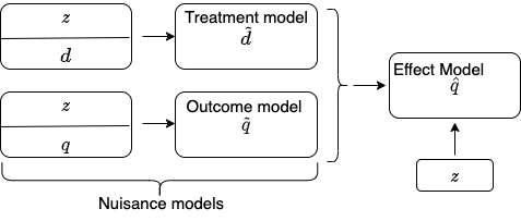
Figure 1: The architecture of the DML Forecaster.

The Nuisance Models

Each of the two nuisance models provide estimates $\tilde{q}$ and $\tilde{d}$ of $q$ and $d$ given $z$ respectively. We call the model that provides $\tilde{q}$ the outcome model and the model that provides $\tilde{d}$ the treatment model. Here, we choose standard transformer-based forecasting models (Vaswani et al. 2017) for their robustness and proven performance in an online retail setting (Eisenach, Patel, and Madeka 2020; Rasul et al. 2021; Zhou et al. 2021a).

Each of the outcome and treatment prediction models have the same architecture and only differ in target and final activation. We use softplus as the final activation function in the outcome model to enforce positivity. For our treatment model, we do not pass the (linear) combination learned by the last layer through a (non-linear) activation function. As we will see from the functional form of the effect model head, this is helpful given the multiplicative nature of the effect model. Around each attention step, there is a residual connection, and after each attention step there is a position-wise feed forward network with layer normalization and dropout. We use an $L1$ loss for training our nuisance models on real-world data and an $L2$ loss when fitting our synthetic data set. Other choices of losses are possible and our approach readily extends to these, in particular for probabilistic scenarios (Gneiting, Balabdaoui, and Raftery 2007).

The Effect Model

The effect model combines the treatment and outcome models to provide the final estimate of demand $q$ in our DML Forecaster which we denote as $\hat{q}$. We now show how our model estimates the price elasticity of demand

$$\epsilon\coloneqq\dfrac{\Delta q}{q}\cdot\dfrac{p}{\Delta p},$$ (4)

where $q$ is demand of an article and $p$ is the price. If we assume mild integrability conditions, then basic integration gives us

$$q_{1}=q_{0}\Big{(}\frac{p_{1}}{p_{0}}\Big{)}^{\epsilon},$$ (5)

where $q_{i}$ is the demand at price $p_{i}$ (see Appendix B for details).

Our idea is to parameterize $\epsilon$ by a neural network. Given retail price $x$, we can write the discounted price as $x\cdot(1-d_{t})$ where $d_{t}$ is the discount at time $t$. Furthermore, we assume that the forecast of the outcome model $\widetilde{q_{t}}$ is an estimate of the sales at the price level predicted by the discount model $x\cdot(1-\widetilde{d_{t}})$. Substituting these into Eq. 5, we can compute our final demand estimate $\widehat{q}$ at time $t$ as

$$\widehat{q_{t}}=\widetilde{q_{t}}\Big{(}\frac{1-d_{t}}{1-\widetilde{d_{t}}}\Big{)}^{\psi(z)}\qquad 1\leq t\leq s,$$ (6)

where $\psi$ is a transformer model whose output is the elasticity $\epsilon$ in (5) and $s$ is the length of the forecast horizon. Note, that while $\epsilon$ is assumed to be constant here, it still is parameterized over $z$ so it can vary by features used in estimation. Our model to parameterize $\epsilon$ is similar to the nuisance models and only lacking the decoder self-attention as we expect elasticity to be relatively constant within the forecast horizon. The outcome model accounts for the auto-regressive part of each time series. We use a negative softplus as final activation as we expect elasticity to be negative (Varian 2014, Chapter 15) and an $L_{1}$ loss for training.

For training the nuisances and effect models, we deploy a two-stage training process, where we fit the nuisance models in the first stage and the effect model in the second stage. The first stage nuisance models generate estimates for the second stage effect models.

To avoid overfitting, we deploy two-fold cross-fitting during training in a similar manner to (Chernozhukov et al. 2017, Section 3). We have an even and odd copy of each nuisance model, each of which are trained on one half of the data set. We use nuisance models trained on odd data to infer outcomes for even data, and vice-versa. This data is used to train a single effect model.

The splitting of the data set into even and odd parts is done according to the index of the item $i$. In the particular instance of demand forecasting, we can derive an index from article information such that articles of the same size are guaranteed to be either even or odd indexed while still having a (close to) random split between different articles.

Inference with the DML Forecaster

Once the model is trained, we need to infer future outcomes for different discount levels. We combine two methods here, one influenced by the above cross fitting procedure and one influenced by standard forecasting methods. We ensemble these two methods with a geometric mean, where $cf$ indicates cross fitting and $f$ indicates forecasting

$$\widehat{q_{t}}=\sqrt{\widetilde{q_{t}^{cf}}\Big{(}\frac{1-d_{t}}{1-\widetilde{d_{t}^{cf}}}\Big{)}^{\psi(z)}\cdot\widetilde{q_{t}^{f}}\Big{(}\frac{1-d_{t}}{1-\widetilde{d_{t}^{f}}}\Big{)}^{\psi(z)}}$$ (7)

In the cross fitting procedure we pass the odd (even) batches to the even (odd) nuisance models, and then receive an inference from the effect model. We do this to account for potentially overfit models.

The standard forecasting practice is to use the model trained on old data to infer future outcomes. To implement this we pass even (odd) batches to the even (odd) nuisance models, and then pass the output to the effect model. This has the advantage of forecasting ahead on items that the nuisance models have seen during training.

Discussion: Departures from the DML Literature

We’re interested in forecasting demand levels for different discount rates. The DML literature is interested in estimating changes in demand levels for changes in discount rates. Although we use cross fitting to train our model, at inference we depart from this, for improved forecast performance. Second, we use a single effect model, instead of separate, averaged treatment effect estimations on each half of the dataset. Third, we use an outcome model that reflects our understanding of the problem space, and not one justified for treatment effect estimation.

4 Experiments

In this section, we present experimental results of the DML Forecaster in a fully controlled setting with synthetic data and on real-world data. We start by discussing practical details around the DML Forecaster.

Baseline Models and Accuracy Metrics

We compare the DML Forecaster to the following models:

• Naïvely-causal Transformer (TF): A time-series transformer architecture with a special output head that models price elasticity more generally than (5) via a piece-wise linear, monotone function (Kunz et al. 2023b).

• SARIMAX: A vanilla seasonal ARIMA model with exogenous covariates. In cases where the training length was less than 30, or the model fitting process failed, we use the previous week’s value as a fallback. For our experiments, we use Darts 0.21.0 (Herzen et al. 2022), co-variates such as stock and discount variables from previous time steps were included, and preprocessing involved log transformation and forward filled for missing values in demand, stock (in $z$), and discounts.

• TWFE elasticities: A standard econometric baseline via a causally informed, elasticity-based forecast using a two-way fixed-effect Poisson regression model (Bergé 2018). Appendix C contains more details.

• sDML: As part of our ablation study, this model implements the DML Forecaster (see Section 3) without the nuisance model for predicting the treatment. Instead the treatment is provided directly to the effect model without residualization.

• No Cross Fitting: Cross fitting is applied to the DML Forecaster as described in Section 3. For our ablation study, we create variants of sDML and DML models without cross fitting (sDML-no cf and DML-no cf).

We have chosen these models to represent the variety of approaches typically deployed for such problems (Januschowski et al. 2020): (i) local forecasting models (SARIMAX), (ii) econometric approaches (TWFE) and (iii) global, transformer-based forecasting methods.

For the accuracy metrics, we use standard metrics mean absolute error (MAE) and mean squared error (MSE) (Hyndman and Athanasopoulos 2017), and the so-called demand error, a metric that captures the down-stream pricing dependency (see Kunz et al. (2023a)):

$$\mathcal{D}_{T,h}=\sqrt{\frac{\sum_{i}\sum_{T=t+1}^{t+h}b_{i}(\hat{q}_{i,T}-q_{i,T})^{2}}{\sum_{i}\sum_{T=t+1}^{t+h}b_{i}q_{i,T}^{2}}}.$$ (8)

Here, $t$ is the last timepoint in the training set, $h$ is the forecast horizon, $\tilde{q}_{i,T}$ is the prediction for article $i$ at timepoint $T$, $q_{i,T}$ is the corresponding true demand and $b_{i}$ is the recommended retail price of article $i$.

Hyperparameter Tuning

The following provides an overview on how we select the hyper-parameters. More details are in Appendix D.

Synthetic Dataset

We use Bayesian optimization (Akiba et al. 2019) to tune key hyperparameters of the DML Forecaster and TF. To mimic a realistic tuning, we use the data of the first 50 weeks of our simulated data whereas we keep weeks 46-50 as a hold out set to select the best hyperparameters, and thus use the first 45 weeks for training. In the case of DML-no cf, we reuse the same hyperparameters found for the DML Forecaster. For sDML and sDML-no cf, we only need to re-tune the effect model, as the nuisance outcome model is used the same way as in our DML Forecaster.

Real-World Data

Both nuisance models have an input dimension of 66, with multiple attention layers in encoder and decoder, and 22 attention heads. The batch size for all nuisance models is $1200$ time series windows, and each had a learning rate scheduler of the form $lr_{n}\mapsto\exp(\alpha)\cdot lr_{n}:=lr_{n+1}\;,$ where $lr_{n}$ is the learning rate in the $n^{th}$ training step.

For the effect model we use twice the batch size as for the nuisance models (2400) which is due to the cross-fitting procedure (see Section 3). Moreover, we use a simple learning rate scheduler of the form

$$lr\mapsto\dfrac{lr}{\sqrt{n+1}}:=lr_{n}$$

where $lr_{n}$ is the learning rate after the $n^{th}$ training step and $lr$ is the initial learning rate.

Experiments on Synthetic Data

	MAE		MSE		MAE effect	MSE effect
Model type	Off policy	On policy	Off policy	On policy
TF	16.3±0.5	11.5±0.4	745.7±38.6	490.6±19.4	45.8±1.0	3350.4±164.6
DML	12.4±0.7	10.0±0.7	658.6±40.6	472.9±33.9	25.0±1.7	1743.9±187.7
DML-no cf	12.4±0.7	10.1±0.7	663.2±49.0	473.6±33.4	22.9±2.7	1458.2±212.9
sDML	20.5±0.5	11.0±0.7	922.3±34.7	501.8±36.0	89.1±0.7	10356.5±251.9
sDML-no cf	20.5±0.6	11.0±0.7	919.4±37.2	499.8±35.7	89.5±1.1	10424.0±219.8

Table 1: Error metrics predicting out-of-sample demand in study of 4500 simulated articles. See text for further details.

We start by providing a high-level overview on the construction of synthetic data to evaluate our approach in a controlled setting (see  Appendix E for further details on the data generating process).

We simulate entire life cycles (100 weeks, typical in the online fashion industry) of around 4500 stock keeping units. Demand in a given week $t$ of article $i$ $q_{i,t}$ is a linear function of price $p_{i,t}$ and an article specific factor $e_{i}$ (treatment effect) as well as a base demand $q_{it}^{(b)}$, i.e.

$$q_{it}=q_{it}^{(b)}+p_{it}\,e_{i}$$ (9)

Here treatment effects $e_{i}$ are article dependent, but constant over time. Note however that elasticity will not be constant over time: $\epsilon_{i,t}=\frac{e_{i}p_{it}}{q_{it}^{(b)}+p_{it}\,e_{i}}$.

The base demand $q_{it}^{(b)}$ is the product of two time dependent components: a noisy trend $\tau_{it}$ that either leads to a linear increase/decrease of demand over the course of the article life cycle, and a seasonality term $s_{it}$:

$$q_{it}^{b}=(\tau_{it}\cdot s_{it}+1)\cdot(c_{i}\,\lambda_{it}+\eta_{it}).$$ (10)

The seasonality has a period of 30 weeks with an article-dependent phase shift in order to simulate different season types. In addition, we scale our time-dependent component with an article-specific factor $c_{i}$ as well as independent additive- and multiplicative noise ($\eta_{it}$ and $\lambda_{it}$ respectively). Note, because of the product form in (10), our simulated noise is scale dependent on the base demand.

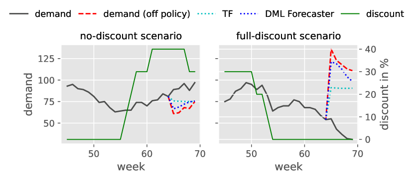
Figure 2: Synthetic demand time series (black), the associated realized discount (green) and off-policy forecasts for DML Forecaster (blue) as well as TF (cyan).

Given our recipe to generate demand, we initialize the simulation for each article $i$ at week $t=0$ by setting an initial stock and price $p_{i1}$. Our goal is to clear the given stock at $t=99$, the season end. We therefore simulate a pricing policy that, at any given week $t>3$, computes the average demand over the past four weeks ($t-1,t-2,\dots,t-4$). We then use this estimate to predict the week number at which the given article $i$ will run out of stock by mere linear extrapolation. If we estimate to clear our stock after $t=99$, we decrease our price by 10% w.r.t. our base price $p_{i0}$ in order to set $p_{it}$. Conversely, if we expect to clear stock before season end, we increase $p_{it}$ by 10%.

Importantly, using such a pricing strategy, treatment is confounded by the long-term seasonal pattern of simulated demand (see example time series in Fig. 2). This leads to higher article discounts when the seasonal component of the simulation is low (Fig. 2, left panel) and lower discounts when seasonal demand is high (Fig. 2, right panel).

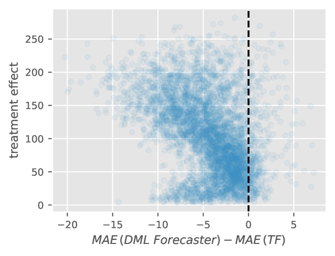
Figure 3: The improvement of the DML Forecaster (the more negative on the x-axis the more improvement) over TF increases with more elastic articles.

We chose a total of four different periods for training: weeks 20-65, 30-75, 40-85, as well as weeks 50-95 and evaluate alternative methods on the five weeks that follow each training interval (weeks 66-70, 76-80, 86-90 and weeks 96-100 respectively). The evaluation consists of two parts: on-policy evaluation, where we predict demand under the pricing policy used in the simulation, as well as off-policy evaluation, where we predict demand under five alternative discount levels that range from 0-50% discount (w.r.t our initial price $p_{i0}$). We repeat training and inference of all models five times to compute empirical standard deviations. In Fig. 2 we show off-policy predictions of the DML Forecaster and TF when applying 0% discount to weeks 65-70 (left panel) and the full discount (50%) respectively (right panel).

In addition to computing the standard metrics MAE and MSE on on- and off-policy ground truth, we also report how accurately our methods predict the treatment effect (MAE effect and MSE effect) – as this parameter is directly modeled and inferred by each of the alternative models.

Model adaptations for this simulation study

Because we deviate from the real-world constant elasticity assumption, we adapt the head effect model as introduced in Eq. 6 accordingly, i.e. our final output is computed as

$$\widehat{q^{t}}=\widetilde{q_{t}}+\psi(z)\cdot(d_{t}-\widetilde{d_{t}})$$ (11)

where $\widetilde{q_{t}}$, $d_{t}$, and $\widetilde{d_{t}}$ are defined as in Eq. 6.

We change TF accordingly, i.e. the head is computed as in Eq. 11, but we set $\widetilde{d_{t}}=0$.

Results

We find that our DML Forecaster (DML) consistently outperforms TF when it comes to predicting demand under off-policy price changes (see Table 1). On policy, the difference between both models is not significant. Furthermore, we find that the advantage of using DML over TF is increasing with the size of the treatment effect (Fig. 3).

Table 1 further contains an ablation study which shows the results of two-stage methods that only learn a nuisance model for predicting demand (sDML and sDML-no cf) and find that they generally perform inferior in off-policy settings and in terms of estimating the effect of price changes.

With this simulation setup, we cannot confirm the benefit of using cross-fitting as the performance of DML and DML-no cf as well as (sDML and sDML-no cf) does not differ significantly across all error metrics we report here (Table 1). We have three explanations for this. First, that the ensembling in (7) removes the benefit of cross fitting. Second, that some residual confounding may be large enough to obscure the benefits of cross fitting. Last, cross fitting is implemented to improve efficiency and statistical power. We may have enough data to fit the model.

Cyberweek: Off-policy Discount Increase

			Off policy				On policy
Target Date	Metric		DML Forecaster	TF	SARIMAX		DML Forecaster	TF	SARIMAX
21-11-2022	Demand Error		61.48	80.03	81.33		60.00	54.73	81.08
23-11-2020			65.94	88.05	78.98		62.50	57.37	78.75
25-11-2019			63.61	63.18	73.03		61.85	57.29	69.59
21-11-2022	MAE		7.739	10.14	9.99		7.606	6.931	9.96
23-11-2020			12.92	17.39	14.82		12.39	11.34	14.78
25-11-2019			12.68	12.52	14.31		12.19	11.40	13.94
21-11-2022	MSE		2047	2540	2225		1903	1940	2196
23-11-2020			5018	7361	4891		5092	5032	5062
25-11-2019			5075	5630	4348		5446	5448	4472

Table 2: Table of metrics for experiment dates considering TF and DML Forecaster for both off and on policy evaluation for cyberweek. All models were trained with an $L1$ loss function. Metrics read from the test epoch output.

One way to test the price response of the models considers certain time periods where the discount policy follows a shifted distribution. In particular, cyber week is such a yearly event when many articles have discounts that are much higher than normally seen during the year. For example, in Fig. 4 we look at the difference in discounts in cyber week 2022 versus two weeks prior at the article level and we see a general right-ward shift, which indicates the general increase in discounting on this special week.

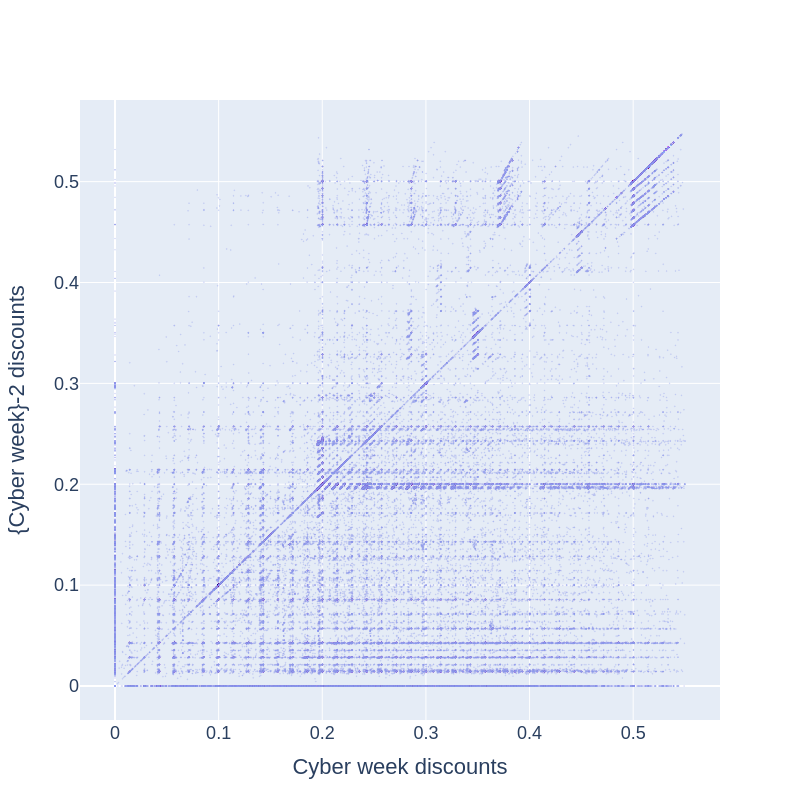
Figure 4: A scatter plot of discounts for articles on cyber week 2022 vs. two weeks prior. Each point represents a single article, and the units on the axes are the ratio of discount, with 0 being no discount and 1 being full discount.

Naturally, similar discount ranges occur during the same week in years prior, so it would not be an interventional test if each model saw these discount-time distributions in training. In order to test our hypothesis, we therefore discard cyber week, cyber week $-1$, and cyber week $+1$ from our training data and replace them with a set of 3 consecutive weeks that are resampled from the same article. We refer to data sets with discarded and replaced weeks as off-policy and to data sets without this replacement as on-policy.

We validate each model on 2021 cyber week, both on- and off-policy, and test each model on 2022, 2020, and 2019 cyber weeks on- and off-policy. Each experiment has a forecast horizon of cyber week and cyber week $+1$, while training on two years of article histories up until cyber week $-1$. The number of articles at inference time was $410,500$ for 2022, $208,212$ for 2020, and $144,980$ for 2019. We give an in depth qualitative description of our data in Appendix F.

Results

As shown in Table 2, we find that the TF has a slight advantage when it comes to predicting demand on-policy, whereas the DML Forecaster yields better results in the off-policy setting, particularly on the MSE. The SARIMAX model is consistently outperformed by both Transformer-based methods.

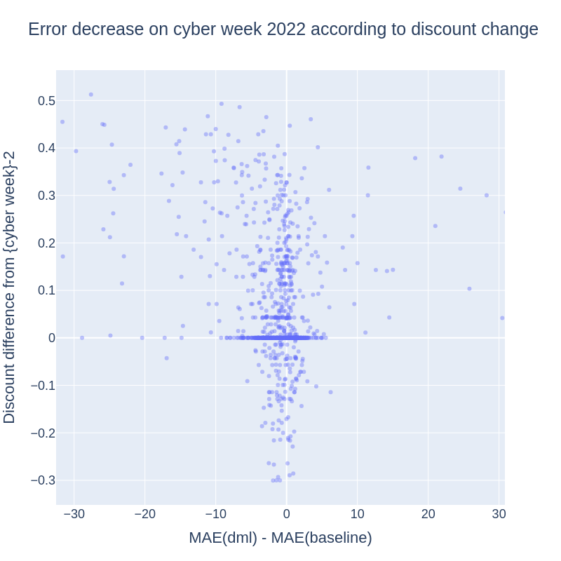
Figure 5: A sample of the difference in forecasting error for the TF vs. DML Forecaster on cyber week 2022, measured on the off-policy experiment.

In addition, we evaluate our methods on control dates not affected by cyber-week sales events (Table 6), and we show how DML improves over TF w.r.t. the degree of discount change (Fig. 5).

5 Related Work

The wider areas of forecasting and causal inference, especially in a pricing context, are well established fields, but typically studied in isolation.

Forecasting with transformers has received considerable attention in the literature in both academic and industrial research (Zhou et al. 2021b; Kunz et al. 2023a; Eisenach, Patel, and Madeka 2020; Lim et al. 2021) and they are generally acknowledged to work well for real-world data sets such as the ones we consider in Section 4. Our approach is generic in the sense that it would work with other transformer-based methods (or indeed, other forecasting methods as long as they allow for the incorporation of covariates). We chose a specific architecture for the ease of implementation and customization to the pricing use case (Kunz et al. 2023a).

In econometrics, demand estimation via price elasticities is of central interest (Deaton and Muellbauer 1980; Fogarty 2010; Hughes, Knittel, and Sperling 2008; DeFusco and Paciorek 2017). Often however, forecasting methods are ignored as the focus is understanding how demand changes when prices or policies change. Recent work has shown how using forecasting algorithms to complement existing econometric techniques can improve causal inference (Goldin, Nyarko, and Young 2022). We do the opposite, using causal inference methods to improve forecast estimates.

Causal forecasting, that is, the intersection of causal inference and forecasting, is typically only mentioned briefly in standard forecasting textbooks (see e.g., (Hyndman and Athanasopoulos 2017)). Similarly, research in causal forecasting is limited to the best of our knowledge. There are some notable exceptions, including the above example using forecasting algorithms to improve causal inference estimates (Goldin, Nyarko, and Young 2022). For example, Vankadara et al. (2022) provide a theoretical framework for differentiating the causal from the statistical risk in forecasting. Our work is more pragmatically oriented in the sense that we do not make assumptions on causal sufficiency (but also do not obtain theoretical guarantees) and rather focus on the empirical validity and evaluation of our approach.

The wider area of estimating counterfactuals is well-studied especially in a medical setting with discrete treatments. Melnychuk, Frauen, and Feuerriegel (2022) recently provide a transformer-based approach for estimating counterfactual outcomes in a discrete treatment setting with medical data. They provide an end-to-end training procedure of three sub-models instead of the multi-stage approach presented here. While a multi-stage approach introduces inefficiencies, the joint loss in (Melnychuk, Frauen, and Feuerriegel 2022) relies on adversarial learning of multiple objectives not in the same domain or scale which is notoriously hard to tune. Our work provides the estimation of a causal parameters of interest, the price elasticity, which (Melnychuk, Frauen, and Feuerriegel 2022) doesn’t yield. Similarly,  Johansson, Shalit, and Sontag (2016) predict patient outcomes over simulated data using a deep neural network approach that corrects for the treatment bias by a given patient’s medical history.  Bica et al. (2020) extend this work to a longitudinal setting, estimating counterfactual patient outcome timeseries while accounting for time-varying confounders. A notable exception is (Pawlowski, Coelho de Castro, and Glocker 2020), where factual information of the period of interest is used in the model in order to compute counterfactuals. Approximating counterfactuals by interventional distributions (Johansson, Shalit, and Sontag 2016; Bica et al. 2020; Melnychuk, Frauen, and Feuerriegel 2022) has the advantage that the resulting methods are by design applicable to interventional settings like ours. Conversely, our proposed approach may also be used to estimate counterfactual outcomes.

6 Conclusion and Future Work

We presented a causal forecasting method in a pricing context via DML. Our model relies on state-of-the-art transformer-based forecasting models and, by incorporating DML, allows for off-policy estimations and a better causal effect estimation than purpose-built, but causally unaware forecasting methods. The evaluation of such forecasts is notoriously difficult and we provide synthetic data as well as natural experiment data for such evaluations.

Future work should include a probabilistic treatment and the incorporation of inverse propensity scores (Lim, Alaa, and Schaar 2018), a more flexible outcome model as well as the inclusion of multi-variate forecasting models.

Causal Forecasting for Pricing: supplemental material

Appendix A Differences Between Cross-fitting and Sample-splitting

Cross-fitting, as deployed in the DML Forecaster, has a primitive method called sample-splitting. This is a simple version of the cross-fitting DML estimation described in literature (Chernozhukov et al. 2017). With the DML Forecaster we split the training data into two randomized subsets (which we refer to as even and odd) as in cross-fitting. However, there is only one of each outcome and treatment model. The nuisance models are trained on the even part of the dataset, while the effect model is trained on the odd part with partial ground truth in (6) provided by the nuisance models’ inference on the odd part. At inference time we use the nuisance and effect models to forecast on the full assortment.

An issue with sample-splitting is that we only use half the dataset for inference. This means that this method is less efficient since it does not use all of the data for training each of the nuisance or effect model.

In our use case there is no shortage of data, and so it becomes a question as to whether this efficiency is really needed. In addition, cross-fitting would add increased training and inference time over sample-splitting. We would like to understand the trade off between the two methods, and therefore designed a small experiment to test the sample-splitting DML model against the cross-fitting DML model, where the former is designed as in the first paragraph in this sub-appendix.

We tested the sample-splitting DML model on the three cyber week start dates, both in and out of sample, and on the control dates in sample in order to compare with the cross-fitting DML model. The hyperparameters for each sub-model in the sample-splitting DML model are taken from the tuning study where cross-fitting was in place. We also measured training time from the tensorboard logs.

The cross-fitting DML Forecaster performed slightly better than the sample-splitting DML Forecaster off-policy. For on-policy, the sample-splitting model performed slightly better than the cross-fitting model on two of the cyber week dates and one of the control dates. On the remaining dates it performed slightly worse. The training time for cross-fitting was significantly longer than that for sample-splitting. See Table 7 for the results.

Appendix B Derivation of Eq. 5

We make the assumption that demand depends negative monotonically on price for a specific article at a specific time, with all other factors being held constant. Further, we assume that elasticity is constant with regard to price, demand, and time. We can then treat Eq. 5 as an equality of differential forms on the positive real line

$$\frac{dq}{q}=\epsilon\frac{dp}{p}.$$

If we integrate both sides over some interval $[p_{0},p_{1}]$,

$$\int_{p_{0}}^{p_{1}}\frac{d(q(p))}{q(p)}=\epsilon\int_{p_{0}}^{p_{1}}\frac{dp}{p}.$$

We can make the substitution of $q(p)=q$ in the left hand side, and get

$$\int_{q_{0}}^{q_{1}}\frac{dq}{q}=\epsilon\int_{p_{0}}^{p_{1}}\frac{dp}{p}$$

where $q_{i}=q(p_{i})$ for $i=0,1$. Thus, we get

$$\log(q_{1})-\log(q_{0})=\epsilon\big{(}\log(p_{1})-\log(p_{0})\big{)}.$$

Exponentiating, we arrive at the result:

$$q_{1}=q_{0}\Big{(}\frac{p_{1}}{p_{0}}\Big{)}^{\epsilon}.$$

Appendix C Elastiticity-based Forecasts

A standard approach to compute demand functions uses estimated elasticities, $\varepsilon$ (see for instance Varian (2014), Deaton and Muellbauer (1980) or Phillips (2021)).

Here, we use estimated elasticities for different groups of articles and past observed demand in order to predict demand for a given week $t$, i.e.

$$\hat{q}_{i,t}=q_{i,t-1}\left(\frac{1-d_{i,t}}{1-d_{i,t-1}}\right)^{\varepsilon}.$$

Due to hidden confounding (e.g., seasonality and advertisement campaigns), naïve regression of $\log(q_{i,\cdot})$ onto $\log(1-d_{i,\cdot})$ generally results in biased estimates of the elasticities. To account for this, we use a two-way fixed-effects Poisson regression model that is defined as follows:

$$\log\big{(}\mathbb{E}[q_{i,t}]\big{)}=\varepsilon\log(1-d_{i,t})+u_{i}+c_{t}.$$ (12)

Here, the parameter $u_{i}$ is the article-specific effect and $c_{t}$ is the week-specific effect. This model is fitted with the standard within estimator using the R package fixest (Bergé 2018).

Appendix D Hyperparameters and Hyperparameter Tuning

Hyperparameter tuning was carried out using the Bayesian search algorithm provided with the python package optuna (Akiba et al. 2019). We provide a full overview of the selected hyperparameters for the TF model in Table 9 and for the DML Forecaster in Table 10. A notable difference between TF and DML Forecaster is that we used RAdam in each DML sub-model and AdamW for the TF model. For tuning the effect model, we trained the nuisance models with optimal hyperparameters and saved a checkpoint of their weights, and then tuned the effect model for its set of parameters without further training of the nuisance models.

Appendix E Simulation Study

In the following, we give more details about the generation of our synthetic data set. Note that, in the main manuscript, we keep our presentation concise and on a high level by omitting the weighting we use for individual components and using a different (but equivalent) parameterization of the noise model.

We simulate a total of 4467 stock keeping units over a period of 100 weeks (i.e $t\in\{0,1,\dots,99\}$). Demand in a given week $t$ of article $i$ ($q_{i,t}$) is a linear function of price $p_{i,t}$ and an article-specific factor $e_{i}$ (treatment effect) as well as a base demand $q_{it}^{(b)}$, i.e.

$$q_{it}=q_{it}^{(b)}+p_{it}\,e_{i}$$ (13)

The base demand $q_{it}^{(b)}$ is the product of two time dependent components: a noisy trend $\tau_{it}$ that either leads to a linear increase/decrease of demand over the course of the article life cycle, and a seasonality term $s_{it}$:

$$q_{it}^{b}=(0.15\cdot\tau_{it}+0.25\cdot s_{it}+1)\cdot c_{it}.$$ (14)

$c_{it}$ is the article-specific contribution that consists of two sub components $a_{it}$ and $b_{it}$:

$$c_{it}=0.05\cdot a_{it}^{2}+0.25\cdot a_{it}+0.5\cdot b_{it}$$ (15)

where

$$a_{it}=\alpha_{d(i)}+\epsilon_{it}$$ (16)

and

$$\alpha_{d}\sim\mathcal{N}(10,\,3^{2})$$ (17)

is sampled once for each category $d\in\{1,2,\dots,45\}$. Furthermore $\epsilon_{it}$ is independent noise drawn from $\mathcal{N}(0,\,1)$ and $d(i)$ is a (random) mapping that assigns article $i$ to one of a total of 45 categories.

The contribution of $b_{it}$ is computed analogously to $a_{it}$ using a different setting of hyperparemeters and a total of 15 categories:

$$b_{it} = \beta_{k(i)}+\psi_{it},\,\psi_{it}\sim\mathcal{N}(0,\,5^{2})$$ (18)

$$\beta_{k} \sim \mathcal{N}(300,\,50^{2}),\,k\in\{1,2,\dots,15\}.$$ (19)

The treatment effect $e_{i}$ in Eq. 14 depends on a random component as well as an article-specific component:

$$e_{i}=e^{(b)}_{i}\cdot 0.15\cdot\bar{a}_{i},\,\,e^{(b)}_{i}\sim\text{max}(1.3,\mathcal{LN}(0.75,\,0.125^{2}))$$ (20)

where $\bar{a}_{i}=\frac{1}{100}\sum_{t=0}^{99}a_{it}$

Furthermore we chose our initial price $p_{i0}$ such that we avoid $q_{it}<0$ at any week $t$:

$$p_{i0}\sim\mathcal{N}\left(\frac{\bar{q}_{i}}{3},\,\left(\frac{\bar{q}_{i}}{1.5}\right)^{2}\right),$$ (21)

where $\bar{q}_{i}=\frac{1}{100}\sum_{t=0}^{99}q_{it}^{(b)}$. We apply additional filtering steps to exclude articles that have negative demand from our synthetic data set. The seasonal component $s_{it}$ in Eq. 14 is a sine function with a period of 30 (weeks) and article-dependent shifts (season types) that are tied to our categorical variable $k$. In particular, we subdivide the values of $k$ evenly into six subgroups and sample season shifts for each group uniformly over all integers in the interval $[-15,15]$.

Lastly, our trend component $\tau_{it}$ follows a (noisy) linear function, i.e.

$$\tau_{it}\sim\mathcal{N}(t\cdot\gamma_{i},\,\sigma_{\tau_{i}}^{2})$$ (22)

where

$$\gamma_{i}\sim\mathcal{U}([-0.02,0.02])$$ (23)

and

$$\sigma_{\tau_{i}}\sim\mathcal{U}([0,0.15]).$$ (24)

With this demand model in place we set our initial stock $z_{0}$ such that we clear our simulated inventory in week $t=99$ at an average discount rate of 14%, i.e

$$z_{0}=\frac{1}{100}\sum_{t=0}^{99}q_{it}^{(b)}\cdot(1-0.14)p_{i0}e_{i}.$$ (25)

Moving along, we compute demand for the first four weeks, i.e $q_{it}$ for $t\in\{0,1,2,3\}$ keeping the price constant ($p_{i0}=p_{i1}=p_{i2}=p_{i3}$). For all weeks $t$ we update our stock accordingly:

$$z_{t+1}=z_{t}-q_{it}$$ (26)

At any given week $t\in\{4,5,\dots 100\}$, we compute the expected number of weeks until we run out of stock ($m_{t}$), via a basic linear extrapolation:

$$m_{t}=\frac{4z_{t}}{\sum_{t_{j}=t-3}^{t}q_{it_{j}}},$$ (27)

which we can use to compute the so-called stock coverage $w_{t}$:

$$w_{t}=\frac{m_{t}}{100-t}.$$ (28)

A value of $w_{t}>1$ implies that demand is too low in order to clear stock at season end, and conversely, a value of $w_{t}<1$ would lead to left over stock after our period of 100 weeks.

Our pricing policy is set up in order to steer $w_{t}$ toward 1 for all $t\in\{4,5,\dots,99\}$. In particular, we define a total of six discount steps $d(j_{t})=j_{t}\cdot 0.1$ for $j_{t}\in\{0,1,\dots,5\}$ for a given week $t$ and adjust our discount step according to the following probabilistic rule:

$$j_{t}=\begin{cases}j_{t-1}+1:w_{t}>1,&\lambda_{ti}>\frac{1}{w_{t}}\\ j_{t-1}-1:w_{t}<1,&\lambda_{ti}>w_{t}\\ j_{t-1}:&\text{ otherwise},\end{cases}$$ (29)

where $\lambda_{ti}\sim\mathcal{U}([0,1])$. We then update our price $p_{it}$ in order to compute demand $q_{it}$ via Eq. 10 as follows:

$$p_{it}=p_{i0}\cdot(1-d(j_{t})).$$ (30)

We give an overview of the synthetic data set and how we derive features from it in Table 3.

Feature	Data type	Notes
Dynamic Features
Demand	Integer $\geq 0$	simulated demand
Discount	Float	range between 0 and 0.5
Stock	Integer $\geq 0$	available stock
Week number	Integer $\geq 0$	week number (embedded)
Positional Encoding	Float(x17)	positional encoding dimensions
Static Features
$d$	Categorical	embedded via a learned embedding
$k$	Categorical	embedded via a learned embedding
Promotion	Binary	noise: not having an effect on demand
$p_{0}$	Integer	undiscounted price of the article

Table 3: Overview of syntetic dataset and its usage with the DML Forecaster and TF

Appendix F Details on Experiments for Real World Data

Qualitative description of our data

Our data consists of sales and other recorded properties of fashion articles that were sold at some point in the past via the retailers online shop. We refer to a single article as Stock Keeping Unit (SKU), and in the following, we consider the so-called config Stock Keeping Units (cSKUs) that group the same articles of different sizes. Thus, all data presented here is agnostic of article size and we ignore effects that are the result of an cSKU being available in a limited number of sizes at some point in its life cycle.

Each cSKU comes with its associated history of weekly-aggregated observations and features. Depending on the context, we use the shorthand cSKU to also refer to a given article’s history. We give more detail on the recorded history and derived features available for each cSKU in Table 4.

Feature	Data type	Notes
Dynamic Features
Sold Items	Integer $\geq 0$	sold items before return
Discount	Float	range between 0 and 0.7
Stock	Integer $\geq 0$	available stock for a given cSKU
Week number	Integer $\geq 0$	iso calendar week number(embedded)
Day in year	Integer $\geq 0$	number of days from January 1st (embedded)
Days from Easter	Integer $\geq 0$	number of days from Easter (embedded)
Positional Encoding	Float(x17)	positional encoding dimensions
Static Features
Brand	Categorical	embedded via a learned embedding
Commodity group	Categorical (x5)	hierarchical category groups (embedded)
Season type	Categorical	season type of article (embedded)
Black price	Integer	undiscounted price of the article

Table 4: Overview of real-world dataset and its usage with the DML Forecaster and TF

Characteristic	Synthetic	Cyber week 2019	Cyber week 2020	Cyber week 2022
No. Time Series	$4,467$	$144,980$	$208,212$	$410,500$
Time Granularity	weekly	weekly	weekly	weekly
Avg. Length of Time Series	$100$	$104$	$100$	$75$
forecast horizon length	$5$	$2$	$2$	$2$

Table 5: High-level characteristics of data sets.

We use one-hot encoding to compute a high-dimensional numeric vector for each categorical feature that we pass through an embedding layer to obtain a low-dimensional representation. Similarly, we use embeddings for our ordinal features (Isoweek number, Days from January first, and Days from Easter). Note, that all embedding layers are an integral part of the neural networks we present here. Thus, during training, we update the parameters of the embedding layers as part of the same gradient update that we use to optimize the remaining weights of each model.

We treat discount as a continuous variable – even though inventory managers typically reduce prices by increments of five percent relative to some baseline (black price). In practice, we need a higher resolution as discounts are recorded as weekly averages. Depending on the time a discount is updated this can result in rather arbitrary decimals. For instance, if the discount for a given fashion item is increased from 20% to 25% in the middle of a given week, we would record a an aggregated discount level of 22.5%.

Further Results

The main cyber-week results are given in Table 2 with the comparison to the control dates given in Table 6. On the 2022 and 2020 cyber weeks, the DML Forecaster performed substantially better across all metrics when compared to the TF model. As we expected, the TF performed mildly better than the DML Forecaster on policy for the cyber weeks. On the 2019 cyber week, the DML Forecaster and TF models performed similarly in the off policy test, and the TF was once again better on policy.

To understand the magnitude of the results with regard to the experiment design, we look at Table 6. Indeed, the degree of change in the error metrics for the TF is not drastic when moving from on policy to off policy for each specific date, when compared to the 2022 and 2020 cyber week dates. The degree of change in the error metrics for the DML Forecaster when considering the on-to-off policy shift is similar to the cyber week dates.

			Off policy			On policy
Target Date	Metric		DML	Baseline		DML	Baseline
	Demand Error
25-04-2022			51.03	57.84		46.55	48.59
06-06-2022			53.76	58.61		47.84	45.61
10-10-2022			52.48	56.18		51.97	51.31
	MAE
25-04-2022			8.935	10.15		8.065	8.478
06-06-2022			7.274	8.081		6.361	6.306
10-10-2022			5.183	5.616		5.078	5.042
	MSE
25-04-2022			1772	2144		1555	1861
06-06-2022			1009	1319		874.0	1007
10-10-2022			510.9	628.0		454.9	507.6

Table 6: Table of metrics for control dates. We consider baseline and DML Forecaster for both on policy and off policy evaluation. All models were trained with an $L1$ loss function. Metrics read from the output of the test epoch.

Further Ablation Study on Real World Data

There are two key elements of the DML Forecaster which are important in avoiding bias (see the Introduction of Chernozhukov et al. (2018) for a deeper discussion). The cross-fitting method allows $\sqrt{n}$-consistency in the linear effect case and prevents the effect model from overfitting. Thus, we can ask if this cross-fitting is necessary in our case: We run the DML Forecaster without cross-fitting and compare to the original, on the start date of 21-11-2022, for both in and out of sample performance. More precisely, we use the even batches with the even nuisance models to provide inference for effect model training, and similarly for the odd version.

As a second experiment, there is a “simplified” version of DML Forecaster (sDML), that does not orthogonalize the treatment function, see for example (Chernozhukov et al. 2018, Equation 1.3). Equation 6 simply becomes

$$\widehat{q^{t}}=\widetilde{q^{t}}\big{(}1-d_{t}\big{)}^{\psi(X)}\qquad 1\leq t\leq s,$$ (31)

where $d_{t}$ is the desired discount. We test this model on the same start date of 21-11-2022.

As a final experiment, we test the sDML model without cross-fitting.

The goal is that this ablation study will help explain the mechanism by which DML Forecaster improves upon the TF for out-of-sample forecasting.

There was not a significant difference between cross-fitting and no cross-fitting for either type of DML Forecaster. The sDML model performed worse on- and off-policy for Demand Error and MAE, regardless of cross-fitting. This is explained by difference in error between the final output and the outcome model. The effect model in the regular DML Forecaster corrected the Demand Error by $6.65$ resp. $2.57$ for off- resp. on-policy over the Demand Error of the outcome model. However, For the sDML model, this correction was significantly less for off policy, and the effect model even increased the error for on-policy. See Table 8 for the results.

		Off policy		On policy		Train time
Target Date	Metric	Cf	Ss	Cf	Ss	Cf	Ss
	Demand Error
21-11-2022		61.48	62.46	60.00	58.41	2.55	1.63
23-11-2020		65.94	68.67	62.50	64.24	1.17	0.71
25-11-2019		63.61	67.52	61.85	61.60	0.83	0.52
25-04-2022				46.55	46.28	1.96	1.27
06-06-2022				47.84	50.26	2.11	1.36
10-10-2022				51.97	52.66	2.44	1.61

Table 7: Demand error for the cross-fitting DML Forecaster compared to the sample-splitting DML Forecaster on the cyber week and control week target dates. Cf = Cross-fitting, Ss = Sample-splitting. Training was done on an AWS Sagemaker instance of type G4dn.4xlarge. Training time is in hours.

				Effect error corr.
Model type	Metric	Off policy	On policy	Off pol.	On policy
	Demand Error
DML		61.48	60.00	-6.65	-2.57
DML-no cf		62.7	60.92	-5.43	-1.95
sDML		64.65	64.34	-3.48	+1.77
sDML-no cf		65.96	65.08	-2.17	+2.51
	MAE
DML		7.739	7.606
DML-no cf		7.883	7.699
sDML		8.144	8.172
sDML-no cf		8.299	8.279
	MSE
DML		2047	1903
DML-no cf		2065	1906
sDML		2067	1899
sDML-no cf		2091	1904

Table 8: Metrics for ablation study for the target date of 21-11-2022. DML-no CF is DML with no cross-fitting, sDML is the simplified DML without the discount residual. Best Metrics for each block are bold. The effect error correction column is the difference in error between the outcome model and the output of the effect model (negative numbers indicate a reduction in error from the outcome model). Metrics read from the output of the test epoch.

Appendix G Details to hardware and library versions used

We performed all experiments using either amazon web services’ (aws) ml.g5.12xlarge instances (simulation study) or g4dn.4xlarge instances (experiments on cyber-week data). The experiments were conducted with PyTorch 2.0.0 and Python 3.10 installed.

Baseline Parameter	Cyberweek Data	Simulated Data	Notes
Number of layers	$6$	$13$	number of residual blocks in the encoder and decoder
Hidden dimension	$274$	$51$	number of hidden dims in ffn after each attention step
Head hidden dimension	$164$	$62$	in the network that computes the normalized demand slopes
Dropout	$0.41$	$0.43$	in all ffns and attention weights
Learning rate	$0.0034$	$0.0224$	for the AdamW optimizer
Weight decay	$0.037$	$1.4\text{\times}{10}^{-4}$	regularization parameter
Beta 1	$0.8044$	$0.8566$	decay rate for computing moving average of gradient in the Adam optimizer
Beta 2	$0.6023$	$0.9140$	decay rate for computing moving average of gradient in the Adam optimizer
Number of linear pieces	$2$	$1$	number of pieces for the demand curve
Train epochs	$2$	$23$
Total parameters	1.3M	124K

Table 9: Hyperparameters for the TF with production data (cyberweek) and simulated data

DML Parameter	Cyberweek Data	Simulated Data	Notes
Outcome model
Number of layers	$3$	$5$	number of residual blocks in encoder and decoder
Hidden dimension	$130$	$73$	number of hidden dims in ffn after each attention step
Dropout	$0.2$	$0.1$	in all ffns and attention weights
Learning rate	$0.0096$	$0.0088$	for the RAdam optimizer
Weight decay	$1.4\text{\times}{10}^{-4}$	$5.4619\text{\times}{10}^{-9}$	regularization parameter
Beta 1	$0.7096$	$0.8566$	decay rate for computing moving average of gradient in the Adam optimizer
Beta 2	$0.8585$	$0.9140$	decay rate for computing moving average of gradient in the Adam optimizer
Gamma	$0.9993$	$0.9388$	Exponential decay of learn rate
Train epochs	$1$	$44$
Treatment model
Number of layers	$2$	$2$	number of residual blocks in encoder and decoder
Hidden dimension	$160$	$21$	number of hidden dims in ffn after each attention step
Dropout	$0.2$	$0.1497$	in all ffns and attention weights
Learning rate	$4.2\text{\times}{10}^{-4}$	$0.0162$	for the RAdam optimizer
Weight decay	$5.8\text{\times}{10}^{-4}$	$2.6\text{\times}{10}^{-09}$	regularization parameter
Beta 1	$0.7884$	$0.5977$	decay rate for computing moving average of gradient in the Adam optimizer
Beta 2	$0.9536$	$0.8740$	decay rate for computing moving average of gradient in the Adam optimizer
Gamma	$0.9995$	$0.9549$	Exponential decay of learn rate
Train epochs	$1$	$60$
Effect model
Number of layers	$5$	$6$	number of residual blocks in encoder and decoder
Hidden dimension	$273$	$43$	number of hidden dims in ffn after each attention step
Dropout	$0.412$	$0.1750$	in all ffns and attention weights
Learning rate	$1.07\text{\times}{10}^{-8}$	$0.0491$	for the RAdam optimizer
Weight decay	$0.0375$	$5.75\text{\times}{10}^{-09}$	regularization parameter
Beta 1	$0.6$	$0.6405$	decay rate for computing moving average of gradient in the Adam optimizer
Beta 2	$0.7044$	$0.6749$	decay rate for computing moving average of gradient in the Adam optimizer
Train epochs	$1$	$20$
Total parameters	1.2M	118K

Table 10: Hyperparameters for the DML Forecaster with production data (cyberweek) and simulated data

References

- Akiba et al. (2019) Akiba, T.; Sano, S.; Yanase, T.; Ohta, T.; and Koyama, M. 2019. Optuna: A next-generation hyperparameter optimization framework. In Proceedings of the 25th ACM SIGKDD international conference on knowledge discovery & data mining, 2623–2631.
- Alexandrov et al. (2020) Alexandrov, A.; et al. 2020. GluonTS: Probabilistic and Neural Time Series Modeling in Python. Journal of Machine Learning Research, 21(116): 1–6.
- Bergé (2018) Bergé, L. 2018. Efficient estimation of maximum likelihood models with multiple fixed-effects: the R package FENmlm. CREA Discussion Papers, (13).
- Bica et al. (2020) Bica, I.; Alaa, A. M.; Jordon, J.; and van der Schaar, M. 2020. Estimating counterfactual treatment outcomes over time through adversarially balanced representations. arXiv preprint arXiv:2002.04083.
- Chernozhukov et al. (2017) Chernozhukov, V.; Chetverikov, D.; Demirer, M.; Duflo, E.; Hansen, C.; and Newey, W. 2017. Double/Debiased/Neyman Machine Learning of Treatment Effects. American Economic Review, 107(5): 261–65.
- Chernozhukov et al. (2018) Chernozhukov, V.; Chetverikov, D.; Demirer, M.; Duflo, E.; Hansen, C.; Newey, W.; and Robins, J. 2018. Double/debiased machine learning for treatment and structural parameters. The Econometrics Journal, 21(1): C1–C68.
- Cunningham (2021) Cunningham, S. 2021. Causal inference: The mixtape. Yale university press.
- Deaton and Muellbauer (1980) Deaton, A.; and Muellbauer, J. 1980. Economics and consumer behavior. Cambridge university press.
- DeFusco and Paciorek (2017) DeFusco, A. A.; and Paciorek, A. 2017. The interest rate elasticity of mortgage demand: Evidence from bunching at the conforming loan limit. American Economic Journal: Economic Policy, 9(1): 210–240.
- Eisenach, Patel, and Madeka (2020) Eisenach, C.; Patel, Y.; and Madeka, D. 2020. MQTransformer: Multi-Horizon Forecasts with Context Dependent and Feedback-Aware Attention. arXiv preprint arXiv:2009.14799.
- Fogarty (2010) Fogarty, J. 2010. The demand for beer, wine and spirits: a survey of the literature. Journal of Economic Surveys, 24(3): 428–478.
- Gneiting, Balabdaoui, and Raftery (2007) Gneiting, T.; Balabdaoui, F.; and Raftery, A. E. 2007. Probabilistic forecasts, calibration and sharpness. Journal of the Royal Statistical Society: Series B (Statistical Methodology), 69(2): 243–268.
- Goldin, Nyarko, and Young (2022) Goldin, J.; Nyarko, J.; and Young, J. 2022. Forecasting Algorithms for Causal Inference with Panel Data. arXiv preprint arXiv:2208.03489.
- Hernán and Robins (2010) Hernán, M. A.; and Robins, J. M. 2010. Causal inference.
- Herzen et al. (2022) Herzen, J.; et al. 2022. Darts: User-Friendly Modern Machine Learning for Time Series. Journal of Machine Learning Research, 23(124): 1–6.
- Hughes, Knittel, and Sperling (2008) Hughes, J.; Knittel, C. R.; and Sperling, D. 2008. Evidence of a shift in the short-run price elasticity of gasoline demand. The Energy Journal, 29(1).
- Hyndman and Athanasopoulos (2017) Hyndman, R. J.; and Athanasopoulos, G. 2017. Forecasting: Principles and Practice. OTexts; 2014. www. otexts. org/fpp., 987507109.
- Januschowski et al. (2020) Januschowski, T.; et al. 2020. Criteria for classifying forecasting methods. International Journal of Forecasting, 36(1): 167–177. M4 Competition.
- Johansson, Shalit, and Sontag (2016) Johansson, F.; Shalit, U.; and Sontag, D. 2016. Learning representations for counterfactual inference. In International conference on machine learning, 3020–3029. PMLR.
- Kunz et al. (2023a) Kunz, M.; Birr, S.; Raslan, M.; Ma, L.; Li, Z.; Gouttes, A.; Koren, M.; Naghibi, T.; Stephan, J.; Bulycheva, M.; Grzeschik, M.; Kekić, A.; Narodovitch, M.; Rasul, K.; Sieber, J.; and Januschowski, T. 2023a. Deep Learning based Forecasting: a case study from the online fashion industry. arXiv:2305.14406.
- Kunz et al. (2023b) Kunz, M.; et al. 2023b. Deep Learning based Forecasting: a case study from the online fashion industry. arXiv:2305.14406.
- Li et al. (2021) Li, H.; et al. 2021. Large-scale price optimization for an online fashion retailer. In Innovative Technology at the Interface of Finance and Operations: Volume II, 191–224. Springer.
- Lim, Alaa, and Schaar (2018) Lim, B.; Alaa, A.; and Schaar, M. v. d. 2018. Forecasting Treatment Responses over Time Using Recurrent Marginal Structural Networks. In Proceedings of the 32nd International Conference on Neural Information Processing Systems, NIPS’18.
- Lim et al. (2021) Lim, B.; Arif, S.; Loeff, N.; and Pfister, T. 2021. Temporal Fusion Transformers for interpretable multi-horizon time series forecasting. International Journal of Forecasting, 37(4): 1748–1764.
- Melnychuk, Frauen, and Feuerriegel (2022) Melnychuk, V.; Frauen, D.; and Feuerriegel, S. 2022. Causal Transformer for Estimating Counterfactual Outcomes. In Chaudhuri, K.; Jegelka, S.; Song, L.; Szepesvari, C.; Niu, G.; and Sabato, S., eds., Proceedings of the 39th International Conference on Machine Learning, volume 162 of Proceedings of Machine Learning Research, 15293–15329. PMLR.
- Pawlowski, Coelho de Castro, and Glocker (2020) Pawlowski, N.; Coelho de Castro, D.; and Glocker, B. 2020. Deep structural causal models for tractable counterfactual inference. Advances in Neural Information Processing Systems, 33: 857–869.
- Petropoulos et al. (2021) Petropoulos, F.; et al. 2021. Forecasting: theory and practice. arXiv:2012.03854.
- Phillips (2021) Phillips, R. L. 2021. Pricing and revenue optimization. Stanford university press.
- Rasul et al. (2021) Rasul, K.; Sheikh, A.-S.; Schuster, I.; Bergmann, U.; and Vollgraf, R. 2021. Multivariate Probabilistic Time Series Forecasting via Conditioned Normalizing Flows. arXiv:2002.06103.
- Seeger, Salinas, and Flunkert (2016) Seeger, M. W.; Salinas, D.; and Flunkert, V. 2016. Bayesian intermittent demand forecasting for large inventories. In Advances in Neural Information Processing Systems, 4646–4654.
- Vankadara et al. (2022) Vankadara, L. C.; Faller, P. M.; Hardt, M.; Minorics, L.; Ghoshdastidar, D.; and Janzing, D. 2022. Causal Forecasting:Generalization Bounds for Autoregressive Models. arXiv:2111.09831.
- Varian (2014) Varian, H. R. 2014. Intermediate microeconomics with calculus: a modern approach. WW norton & company.
- Vaswani et al. (2017) Vaswani, A.; Shazeer, N.; Parmer, N.; Uszkoreit, J.; Jones, L.; Gomez, A. N.; Kaiser, Ł.; and Polosukhin, I. 2017. Attention is all you need. Advances in Neural Information Processing Systems (NIPS 2017), 30.
- Wen et al. (2017) Wen, R.; Torkkola, K.; Narayanaswamy, B.; and Madeka, D. 2017. A multi-horizon quantile recurrent forecaster. In NIPS 2017 Time Series Workshop.
- Zhou et al. (2021a) Zhou, H.; Zhang, S.; Peng, J.; Zhang, S.; Li, J.; Xiong, H.; and Zhang, W. 2021a. Informer: Beyond Efficient Transformer for Long Sequence Time-Series Forecasting. arXiv:2012.07436.
- Zhou et al. (2021b) Zhou, H.; et al. 2021b. Informer: Beyond Efficient Transformer for Long Sequence Time-Series Forecasting. In The Thirty-Fifth AAAI Conference on Artificial Intelligence. AAAI Press.