Adaptive Reduced Multilevel Splitting

Abstract

This paper considers the classical problem of sampling with Monte Carlo methods a target probability distribution obtained by conditioning on a rare event defined by the level set of a real-valued score function that is very expensive to compute. We also consider a context where, with each new evaluation of the true score function, a method that iteratively builds a sequence of reduced scores is available; these reduced scores being moreover certified with pointwise error bounds. This work proposes a fully adaptive algorithm that iteratively: i) builds a sequence of proposal distributions obtained by conditioning on the reduced score above an adaptively well-chosen level, and ii) draws from the latter both for importance sampling of the true target rare events, as well as for proposing relevant (expensive) updates to the reduced score. An essential contribution consists in the adaptive choice of the level in i) and ii). The latter is calculated solely from the reduced score and its error bound, and is interpreted as the first non-achievable level as quantified by a given cost (in a pessimistic scenario) of importance sampling of the associated true target distribution. From a practical point of view, sampling the proposal sequence is performed by extending the framework of the popular Adaptive Multilevel Splitting (AMS) algorithm to the use of score function reduction. Numerical experiments evaluate the proposed importance sampling algorithm in terms of computational complexity versus squared error. In particular, we investigate the performance of the algorithm when simulating rare events related to the solution of a parametric PDE approximated by a reduced basis.

1 Introduction

1.1 Context

Let $\left(\eta^{\ast}_{l}\right)_{l\in\mathbb{R}}$ denote a family of target probability distributions defined on a state space $\mathcal{X}$ by the conditional probability distributions

$$\eta^{\ast}_{l}\displaystyle\mathop{=}^{{\rm def}}\frac{1}{p_{l}^{\ast}}\,{\rm l}{\rm l}_{S^{\ast}>l}\mathrm{d}\pi,\qquad l\in\mathbb{R}.$$ (1.1)

In the above, $\pi$ denotes a given, easily simulable, reference probability distribution, and

$$S^{\ast}:\mathcal{X}\to\mathbb{R},$$

denotes a real-valued score function. This score function is assumed to be of the form

$$S^{\ast}(x)=\mathrm{score}(\Psi^{\ast}(x)),$$

where $\mathrm{score}$ is an easily computable function of physical interest, and $\Psi^{\ast}(x)$ is the outcome of a presumably exact numerical computation of a complex physical system parametrized by $x\in\mathcal{X}$. For instance, the random variable $x$ can describe unknown physical parameters, uncertainty on initial/boundary conditions, or additional noise modeling either a chaotic behavior or the interaction with an environment. The quantity $p^{\ast}_{l}\displaystyle\mathop{=}^{{\rm def}}\int_{\mathcal{X}}\,{\rm l}{\rm l}_{S^{\ast}>l}\mathrm{d}\pi=\pi\left(\left\{S^{\ast}>l\right\}\right)$ is the associated normalization, here the probability of the considered rare events $\left\{S^{\ast}>l\right\}$, for $l\in\mathbb{R}$.

We consider the classical problem of designing an algorithmic Monte Carlo procedure that samples according to $\eta^{\ast}_{l_{\mathrm{max}}}$ – for one specific large $l_{\mathrm{max}}\in\mathbb{R}$ – and estimate the associated rare event probability $p^{\ast}_{l_{\mathrm{max}}}$ (the normalization).

In this work, we will be interested in scenarios in which the practitioner has to face two types of difficulty.

The first difficulty is classical – especially for high dimensional multimodal landscapes, and arises when $l$ increases, yielding a rare event (or low temperature) problem, similar to global optimization. A rare event problem is defined by a very small yet strictly positive probability $p^{\ast}_{l}$; the analogue in statistical mechanics being the low temperature regime. Both settings confronts the practitioner with similar computational challenges: the density defining $\eta_{l}^{\ast}$ concentrates the majority of the probability mass in specific but unknown areas of $\mathcal{X}$, which are roughly described by the maxima of $S^{\ast}$. A direct sampling with a Monte Carlo simulation of $\pi$ requires a sample size of order at least $1/p^{\ast}_{l}$, which is often infeasible. In that context, a very popular general strategy to simulate a sample according to $\eta^{\ast}_{l}$ and to estimate the associated normalizing constant is to resort to a Sequential Monte Carlo (SMC) strategy (see [10]) that starts with a Monte Carlo sample of particles distributed according to $\pi$ and then sequentially samples $\eta^{\ast}_{l}$ for increasing values of $l$ by resorting to a combination of Importance Sampling (IS), re-sampling (selection) of weighted samples and mutations of particles based on suitable Markov Chain Monte Carlo transitions. More specifically, we are interested in an adaptive variant designed for the rare event context, namely the Adaptive Multilevel Splitting (AMS) algorithm (see [5]). Some reader may find convenient to note that AMS is a close relative to subset simulation [1].

The second difficulty we will consider here appears when the numerical evaluation of $\Psi^{\ast}$ is extremely expensive; so expensive that the number of evaluations required in, say, a usual SMC approach becomes prohibitive. In order to circumvent this issue, we assume that the physical model $\Psi^{\ast}$ can be approximated by a reduced model denoted $\Psi$; the cost of evaluating $\Psi$ being small as compared to one evaluation of the true score with $\Psi^{\ast}$. The reduced model $\Psi$ we consider is assumed to come with two key features. To explain these, let us denote from now on the approximate score function by

$$S(x)=\mathrm{score}\left(\Psi(x)\right)\in\mathbb{R}.$$

The first feature is an a posteriori pointwise error quantification associated with $S$. This error quantification comes in the form of an error bound denoted

$$E(x)=\mathrm{error}\left(\Psi(x)\right)\in\mathbb{R},$$

and satisfying the pointwise estimate:

$$\left|S(x)-S^{\ast}(x)\right|\leq E(x),\qquad\forall x\in\mathcal{X}.$$ (1.2)

The second key feature assumes that we are able to update the reduced model, through a procedure of the following form

$$\left\{(X_{1},\Psi^{\ast}(X_{1})),\ldots,(X_{k},\Psi^{\ast}(X_{k})\right\}\xmapsto{\textrm{reduced model}}\Psi=\Psi^{(X_{1},\ldots,X_{k})},$$

which takes as an input any sequence of states in $\mathcal{X}$ – called here a sample of snapshots – together with the solution of the associated true model $\Psi^{\ast}$ evaluated for each of those snapshots. The output is the reduced model $\Psi$. In order to improve the readability, and throughout the paper, we may use the superscript $(k)$ instead of $(X_{1},\ldots,X_{k})$, or even drop it, as follows:

$$(S^{(X_{1},\ldots,X_{k})},E^{(X_{1},\ldots,X_{k})})=(S^{(k)},E^{(k)})=(S,E),$$

and we will proceed equivalently for any quantity that depends on the model reduction procedure through $(X_{1},\ldots,X_{k})$, the sample of snapshots.

A reduced model can be constructed by various, potentially very different, means. In this work, we will consider the reduced modeling procedure and its error quantification satisfying (1.2) as a black box. However, the numerical tests will be performed with two specific reduced modeling approach. The first test, based on splines, is artificially challenging (for the simulation method) and is not meant to be used in practice. The second test uses a reduced basis model reduction. Both rigorously satisfy  (1.2).

1.2 Previous works

Reduced modeling

The idea of using a simpler surrogate model in Monte-Carlo simulation for target distributions is not new and there is a large amount of literature on the subject. Most references are concerned with either kriging on the one hand, and reduced basis methods on the other hand.

A popular Bayesian approach is given by kriging, in which the surrogate score function $S:\mathcal{X}\to\mathbb{R}$ is a random field, distributed according to the posterior of a prior Gaussian field conditioned by fitting the exact values of the evaluated snapshots. The estimate (1.2) is however not satisfied almost surely, and one has to resort to averaged error estimates.

Among deterministic approaches, we will especially be interested in reduced basis methods, which are known to be very efficient for the numerical approximation of problems involving the repeated solution of parametric Partial Differential Equations (PDEs). The strategy adopted consists in projecting the associated high dimensional numerical problem on a subspace where the solutions corresponding to suitably chosen parameters are efficiently approximated and characterized with precise error bounds of the form (1.2). An overview on the theoretical rationale behind reduced basis and the practical application of this method is provided in the reference book [21].

The list of references having connections with our work and using kriging is the following: [11, 19, 22, 25, 2, 17, 3], while those using reduced basis is [8, 16, 13, 15]. Generic or other meta-models are considered in [4, 12, 24, 20]; the special problem of well-tuning a combination of possibly generic multiresolution or multifidelity surrogates is treated in [12, 24], as well as in the survey [20].

Snapshot sampling

Arguably, the most sensitive feature of such reduced model approaches to sampling is the specific collection of snapshots (with associated evaluation of the true model) $(X_{k},\Psi^{\ast}(X_{k}))$, $k\geq 1$ with which the reduced model is updated after each iteration $k$. A natural adaptive approach in this context consists in sampling sequentially the collection of snapshots, the reduced model being updated after each iteration $k$. The updated reduced model (and its associated error estimates) can then be used to pick the next snapshot in presumably interesting areas.

The sampling or selection of snapshot $X_{k}$ then follows from two ingredients: i) a probability distribution used to generate candidates, and ii) a weighting or fitness function (sometimes called learning function) used to pick the presumably best candidate. The idea of ingredient ii) can be found in the seminal work of [11] where selecting snapshots is called active learning. In the latter approach, snapshots are selected by optimizing a criterion (the learning function) that will most likely reduce the uncertainty of the kriging surrogate model. An exhaustive set of references and a very quantitative review of methods related to active learning and kriging is provided in [19]. Some other references, as [16], pick the snapshots $(X_{k})_{k\geq 1}$ uniformly among candidates using a decreasing sequence of subsets that contain the target rare event, constructed using the iteratively updated error estimates.

As we will argue in the present work, ingredient i) is also of high importance. Indeed, a key general phenomenon in a rare-event and high-dimensional setting is the following: the true target distribution $\eta^{\ast}_{l}$ is extremely concentrated around very specific but unknown points in $\mathcal{X}$, so that, unless the pool of candidates among which snapshots $(X_{1},\ldots,X_{k})$ are picked is partly also located in the same regions, the information given by the reduced model $\Psi^{(X_{1},\ldots,X_{k})}$ may not be accurately updated. As a consequence, unless one is ready to sample an unreasonable amount of candidates used to optimize the learning function, it is critical to select such candidates in areas that carefully “approach” the true rare event. Note also that sampling the snapshot with a well-identified distribution (instead of an optimization procedure) enables to perform importance sampling with the exact model $S^{\ast}$; an approach we will use in the present work.

Most references in the literature (at least those cited here) construct pools of candidates for the choice of snapshot $X_{k}$ at iteration $k$ by relying on either the reference distribution $\pi$ (in an offline or preliminary phase), or (in some way or another) on the history of states resulting from sampling at iteration $k$ surrogates of the target conditional distributions (1.1) built using the reduced score, defined by

$$\mu_{l}\displaystyle\mathop{=}^{{\rm def}}\frac{1}{Z_{l}}\,{\rm l}{\rm l}_{S>l}\mathrm{d}\pi\qquad l\in\mathbb{R}.$$ (1.3)

Again, a potential issue is that for large $l$, the reduced rare event is also rare, hence very concentrated, and thus usually off, being too far away from the true target rare event. Selecting carefully an appropriate specific $l$ by leveraging the existence of error estimates is a key novelty introduced in the present work. This delicate issue is addressed in very few papers in the literature. In a reverse approach, let us mention the worst-case error criterion proposed in [15], which is used to select the reduced score $S$ in a hierarchy of precomputed surrogates, given some level $l$.

Sampling the reduced rare event

The general framework discussed above has been used extensively for rare event simulation in conjunction with several Monte Carlo strategies used to sample the reduced conditional distributions $\mu_{l}$. Sampling strategies can be grouped in two broad categories: on the one hand importance sampling (IS), usually through a parametric approach (a popular advanced method being e.g. adaptive IS with cross entropy minimization), and on the other hand split/ subset / adpative multilevel splitting (AMS) / sequential Monte Carlo (SMC) simulation methods which are non-parametric (albeit targeting an approximate, surrogate distribution).

Let us present a brief review of recent contributions that exploit this general framework of adaptive surrogate modeling for rare event simulation. We will consider IS approaches on the one hand and AMS simulation on the other.

Many adaptive approaches to importance sampling have been proposed in recent years. In particular, a popular criterion for finding a good proposal in a parametric family is obtained by minimizing the relative entropy between the target and the proposal, resulting in the cross-entropy method ([9]). This method has been proposed for surrogate targets based on kriging in [2], or reduced basis approximations in [13, 15]. Other recent contributions also builds adaptive proposals for IS using kriging models [22, 25]. In order to increase the effectiveness of the cross-entropy method, let us mention that it has been suggested to approximate the parameter variable $X$ by constraining its support in well-chosen low dimensional subspaces of $\mathcal{X}$ [23]. Stratified sampling (that can be interpreted as a form of IS) with a surrogate model is developed in [4].

Similarly to adaptive IS, sampling with splitting methods (subset simulation, AMS) have been used in conjunction with kriging-based surrogate models (constructed adaptively) in [17, 3]. We refer again to the review on methods related to active learning and kriging provided in [19]. In [12] subset simulation is performed using nested multiresolution sets (provided by an accuracy hierarchy of the surrogate model), yielding an estimate with an associated a posteriori error. Instead of targeting distributions defined by conditioning on surrogate rare events, one can also use sequential Monte Carlo with soft levels and tempering. This is the approach chosen in [24] with a score function also relying on a multiresolution approximation of a PDE solution.

Adapting splitting methods to reduced scores generally requires the definition of a bridging procedure. The goal of this bridge is to sample a new proposal $\mu^{\prime}_{l^{\prime}}$ defined with some updated reduced score ${S}^{\prime}$ and level $\l^{\prime}$, starting from the samples of the current proposal $\mu_{l}$. In general, this sampling is not trivial. For example, the nesting underlying an AMS algorithm is broken, since in general updating the reduced score and the level will imply $\left\{{S}^{\prime}>l^{\prime}\right\}\not\subset\left\{S>l\right\}$. There is very little work in the literature on this bridging problem. However, we would like to mention the work [24], which proposes a bridging procedure in the context of subset simulation with a level $l^{\prime}=l$ maintained along the bridge.

1.3 Sketch of the proposed method

In this work, we will consider the surrogates of the target conditional distributions (1.1) built using the reduced score as proposal distributions, in the sense of importance sampling. The latter are defined by (1.3), in which the normalization probability $Z_{l}\displaystyle\mathop{=}^{{\rm def}}\int_{\mathcal{X}}\,{\rm l}{\rm l}_{S>l}\mathrm{d}\pi$ represents an approximation of the probability $p^{\ast}_{l}$ of the true rare event. The main iteration index of the main algorithm is $k$, the total number of sampled snapshots already evaluated with the true model. The main algorithm is basically the following.

• The simulation of importance or proposal distributions $\mu_{l}$ at various level $l$ is implemented using an AMS Monte Carlo methodology, in which $\mu_{l}$ is approximated by the empirical distribution of a sample of particles.

• At each iteration $k$, the snapshot $X^{(k+1)}$ is chosen among the sample of particles (which become candidates) when distributed according to the importance distribution $\mu_{l^{(k)}}$, with a well-chosen level $l^{(k)}$. It will be necessary in early stages of the algorithm to replace the uniform sampling of $X^{(k+1)}$ among particles by a penalized sampling based on a learning function, for instance by adding probability weights to states with high errors, as discussed in Section 2.3.

• The true model is evaluated at $X^{(k+1)}$ and the reduced model is updated accordingly.

• Importance sampling estimators of the target rare event problem are provided using the sequence of snapshots $(X^{(k)},\Psi^{\ast}(X^{(k)}))_{k\geq 1}$.

The main methodological contribution of the present work is the specific choice of the level $l^{(k)}$. At each iteration $k$, we will use the information given by the error quantification in order to adaptively choose a level $l^{(k)}$ so that $\mu_{l^{(k)}}^{(k)}$ remains a reasonable importance distribution associated with the true target $\eta^{\ast}_{l^{(k)}}$. This way, we follow (using the AMS methodology here) the concept of rare event sequential sampling along the flow of targets $l\mapsto\eta^{\ast}_{l}$. However, because we rely on a surrogate model when sampling according to $\mu_{l^{(k)}}^{(k)}$, we stop the increase of rareness of the targets when the reduced modeling becomes critically inaccurate, the associated level being denoted $l:=l^{(k)}$. Snapshot (true model) sampling is then preformed using a sample of candidates following $\mu_{l^{(k)}}^{(k)}$, considered at the precise level $l^{(k)}$ of the flow where increasing the quality of the reduced model becomes necessary. By doing so, we ensure that the choice of the snapshot will be consistent with the unknown target, albeit for a moderately large level $l^{(k)}$.

The evaluation of the accuracy of an importance distribution will be done using a quantification of the following logarithmic cost of importance sampling by relative entropy:

$$\ln\mathrm{cost}\simeq\mathrm{Ent}(\eta_{l^{(k)}}\mid\mu^{(k)}_{l^{(k)}})\displaystyle\mathop{=}^{{\rm def}}\eta_{l^{(k)}}(\ln\frac{\eta_{l^{(k)}}}{\mu^{(k)}_{l^{(k)}}}),$$

discussed and justified in Appendix A. The latter cannot be evaluated exactly, but we can leverage the existence of error estimates in order to obtain (more or less pessimistic) approximations of it.

Remark that the more one learns about the true score $S^{\ast}$ by generating snapshots, the more we improve the reduced model (for specific, well-chosen rare states), the more we may reduce the cost of importance sampling. When this happens, the log-cost criteria limiting the level $l$ to $l^{(k)}$ is alleviated, and the algorithm is likely to increase the level beyond $l^{(k)}$ in subsequent iterations.

The proposed method enables to obtain importance sampling estimators. If for instance the snapshots are sampled according to importance distribution $X^{k+1}\sim\mu^{(k)}_{l^{(k)}}$ from the start, it naturally leads to the following estimator:

$$\hat{\pi}^{(k)}\displaystyle\mathop{=}^{{\rm def}}\frac{1}{k}\sum_{k^{\prime}=1}^{k}\frac{\mathrm{d}\pi}{\mathrm{d}\mu^{(k^{\prime}-1)}_{l^{(k^{\prime}-1)}}}(X^{(k^{\prime})})\delta_{X^{(k^{\prime})}},$$ (1.4)

which by construction, is an unbiased empirical estimator of the reference distribution $\pi$ (see Section 3.2), up to sampling errors of the proposal $\mu_{l}$ by AMS. This leads to unnormalized estimators of the target $\eta^{\ast}_{l}$ by evaluating

$$\hat{\pi}^{(k)}(\varphi\,{\rm l}{\rm l}_{S^{\ast}>l}),$$

for various $l$ and test function $\varphi$, which can be easily done because the true score of each snaphots has been evaluated preliminarily by construction of the algorithm; in particular

$$\hat{p}=\hat{\pi}^{(k)}(\,{\rm l}{\rm l}_{S^{\ast}>l}).$$

As mentioned above, the sequence of importance distribution $\mu_{l^{(k)}}^{(k)}$ will be simulated by a population of particles and an AMS methodology in the spirit of current rare event simulation algorithms. The only difference is that the target distribution is constructed with a reduced score that is adaptively enriched by few evaluations of the true score throughout the simulation. An important remark is that updating the reduced score will in general break the nesting of the sequence of distributions. A simple way of addressing this problem is to perform a fresh AMS simulation each time that a new snapshot is picked and that the reduced score is updated. To significantly reduce the number of evaluations of the reduced model, another option is to propose a bridging procedure. This is the second main methological contribution of this work. At iteration $k$, this procedure searches in the simulation history for a well-chosen previous proposal denoted $\mu_{l^{(k_{\mathrm{bridge}})}}^{(k_{\mathrm{bridge}})}$ with $k_{\mathrm{bridge}}\leq k$, so that the updated proposal denoted $\mu_{l_{\mathrm{bridge}}(k+1)}^{(k+1)}$, with ${l_{\mathrm{bridge}}(k+1)}$ a well-designed level, is dominated by and sufficiently close to the former. The latter proposal is then simulated starting from the former one using an AMS framework.

In numerical experiments, we study the proposed algorithm, called Adaptive Reduced Multilevel Splitting (ARMS) in the context of these two variants: fresh AMS simulation or bridging. We show the empirical convergence of the ARMS algorithm on a toy model and a rare-event problem based on a more realistic PDE. Our study confirms that the proposed relative entropy criterion plays a crucial role in ARMS and prevent the simulation to be taken into spurious regions of the state-space remote from the region of interest, resulting in a large variance of the IS estimator. Moreover, by evaluating the computational complexity in relation to the squared error of the estimate, we show empirically that the bridging procedure significantly reduces the simulation cost while achieving a comparable squared error.

The paper is organized as follows. The main methodological concepts underlying the ARMS algorithm are presented in Section 2. We then introduce an idealized version of the ARMS algorithm in Section 3, which assumes the exact evaluation of expectations and exact sampling of distributions. In Section 4, we define ARMS, which consists in a practical implementation of this idealized algorithm using AMS simulations. In Section 5, we numerically evaluate the proposed algorithm for two rare event problems. A final section deals with conclusions and perspectives. The appendix collects some technical proofs and details.

2 Underlying Methodological Concepts

2.1 Importance sampling cost

Let $l_{\max}$ denote a large level of interest, and let us assume for the sake of the argument within the present section, that one is able to simulate a random variable $X$ distributed according to the proposal distribution $X\sim\mu_{l}=\frac{1}{Z_{l}}\,{\rm l}{\rm l}_{S>l}\mathrm{d}\pi$, the normalization $Z_{l}$ being known. Importance sampling of the target rare event $\left\{S^{\ast}>l\right\}$ can be performed in our context if the distribution $\mu_{l}$ dominates the measure $\,{\rm l}{\rm l}_{S^{\ast}>l}\mathrm{d}\pi$, and simply amounts to remark that one can estimate the averages

$$Z_{l}\mathbb{E}\left[\,{\rm l}{\rm l}_{S^{\ast}(X)>l}\varphi(X)\right]=\pi\left(\varphi\,{\rm l}{\rm l}_{S^{\ast}>l}\right),$$

where $\varphi$ denotes a generic test function. For instance taking $\varphi=\,{\rm l}{\rm l}$, the above yields an unbiased estimator of the normalization probability $p^{\ast}_{l}$.

The domination requirement, denoted

$$\mu_{l}\gg\eta_{l}^{\ast},$$

holds true by definition if and only if one has the inclusion $\left\{S^{\ast}>l\right\}\subset\left\{S>l\right\}$. This is not guaranteed here as $S$ is an approximation of the true score $S^{\ast}$, and since $S^{\ast}$ is not computed for each sample states, one cannot check it in a systematic fashion. However, as we will discuss in the next section, the error bound $E$ can be used to propose a sufficient condition corresponding to a worst case scenario.

Unfortunately, even if the above domination condition holds, importance sampling becomes quickly infeasible if the target distribution diverges too widely from the proposal, a typical phenomenon in high dimension. As discussed in Appendix A, it has been thoroughly argued in [7] (see also [6]) that the cost of importance sampling – in terms of the required sample size $K$– is quite generically and roughly given by the exponential of the relative entropy between $\eta^{\ast}_{l}$ and $\mu_{l}$:

$$K\simeq\mathrm{e}^{\mathrm{Ent}(\eta^{\ast}_{l}\mid\mu_{l})}.$$ (2.1)

This fact will justify the choice of various heuristics that will be found in this paper. We will call $\mathrm{Ent}(\eta\mid\mu)$ the log cost of importance sampling of the target $\eta$ by the proposal $\mu$. In the present rare event case, note that relative entropy is simply the logarithm of small probability ratios $\mathrm{Ent}(\eta^{\ast}_{l}\mid\mu_{l})=\ln\frac{Z_{l}}{p^{\ast}_{l}}$, the domination condition ensuring $Z_{l}\geq p^{\ast}_{l}$.

Note that domination between measures is implied by finite relative entropy, and will rather use throughout the paper the condition

$$\mathrm{Ent}(\eta\mid\mu)<+\infty$$

in order to check the domination condition $\mu\gg\eta$.

2.2 First non-achievable level

In this section, we describe how to choose the target level $l^{(k)}$, which is suited to the current score function $S^{(k)}$ at iteration $k$ ($k$ being the number of newly sampled snapshots of the true model) of the main loop of the algorithm. The idea is to tune $l^{(k)}$ with a criteria evaluating that surpassing this level should require, in some sense, a better surrogate model, and thus new snapshots. The adjusted proposal $\mu^{(k)}_{l^{(k)}}$ will then be used to a sample a new snapshot, and obtain an updated score function $S^{(k+1)}$ for the next iteration $k+1$. In short, we are going to develop a heuristic criterion on levels to detect when and where a new snapshot is needed.

The general insight is the following. Consider the following simpler problem: one is given a family of rare event target distributions $\left(\eta^{\ast}_{l}\right)_{l\in\mathbb{R}}$ in the form of (1.1), a given computational budget, and a family of importance sampling proposal distributions $(\mu_{l}^{(k)})_{l\in\mathbb{R}}$ in the form of (1.3). One wants to perform some sequential algorithm to sample the distributions $\mu_{l}^{(k)}$ along an increasing sequence of levels $l$ as high as possible, and then use importance sampling. However, we do not want to waste resources for levels that are ”unreasonably” high. As an idealized criteria giving achievable levels, we propose the importance sampling cost (2.1) of the true target. The first non-achievable (hence critical) level is thus given when the latter matches a certain given numerical threshold $e$: loosely speaking,

$$\text{Find first}\,l:\quad\mathrm{Ent}(\eta^{\ast}_{l}\mid\mu^{(k)}_{l})\geq e.$$

By doing so, we ensure that the snapshot sampled with respect to $\mu_{l}^{(k)}$ will not diverge too much from a meaningful target distribution $\eta^{\ast}_{l}$ with an appropriate level $l$. As an example, if, as it is the case in the present context, $\mu_{l}^{(k)}$ has been constructed using a reduced model based on $k$ snapshots $(X_{1},\ldots,X_{k})$, it is unlikely that it can be used as an importance proposal for levels higher than $\max(S^{\ast}(X_{1}),\ldots,S^{\ast}(X_{k}))$, as the quality of the approximation $S^{\ast}-S^{(k)}$ will deteriorate in areas with higher scores.

In a practical context, the log cost $\mathrm{Ent}(\eta^{\ast}_{l}\mid\mu_{l}^{(k)})$ has to be estimated using some prior information on $\eta^{\ast}_{l}$, for instance using some form of error quantification. We propose in this work the following method, which is by no means unique. We consider a pessimistic (respectively an optimistic) surrogate of $\eta^{\ast}_{l}$, denoted by $\check{\eta}_{l}^{(k)}$ (respectively by $\hat{\eta}_{l}^{(k)}$), constructed with the reduced score $S^{(k)}$ and its error quantification $E^{(k)}$, and associated with a much lower (respectively higher) rare event probability than $\eta^{\ast}_{l}$. In the present work, we will choose (2.3)-(2.4) below which even satisfy:

$$\check{\eta}_{l}^{(k)}\ll\eta^{\ast}_{l}\ll\hat{\eta}_{l}^{(k)}$$

The first non-achievable level will be estimated using the pessimistic surrogate by searching the closest level such that the log cost $\mathrm{Ent}\left(\check{\eta}_{l}^{(k)}\mid\mu_{l}^{(k)}\right)$ matches the threshold $e$. Given an initial level $l_{0}$, this yields the following rigorous definition of the (critical) first non-achievable level:

$$l^{(k)}(e,l_{0})=\min\{l\geq l_{0}:\;\mathrm{Ent}\left(\check{\eta}_{l}^{(k)}\mid\mu_{l}^{(k)}\right)\geq e\;\;\text{or}\;\;\mathrm{Ent}\left(\hat{\eta}_{l_{\mathrm{max}}}^{(k)}\mid\mu_{l}^{(k)}\right)=+\infty\}.$$ (2.2)

$l(e,l_{0})$ is a level such that, in the (unfortunate) case where the true target is given by the pessimistic choice $\check{\eta}_{l}^{(k)}$, a log cost of $e$ is necessary and sufficient in order to perform importance sampling. Note that the last inequality constraint in (2.2) is added to ensure that the support of $\mu_{l}^{(k)}$ includes the support of the final target ${\eta}^{\ast}_{l_{\mathrm{max}}}$.

In the present rare event case where for $l\in\mathbb{R}$, the target is given by (1.1) and the importance distribution by (1.3) with pointwise error bounds (1.2), we propose the pessimistic and optimistic surrogate targets

$$\check{\eta}_{l}^{(k)}\displaystyle\mathop{=}^{{\rm def}}\frac{1}{\check{Z}_{l}^{(k)}}\,{\rm l}{\rm l}_{S^{(k)}-E^{(k)}>l}\mathrm{d}\pi\quad\textrm{with}\quad\check{Z}_{l}^{(k)}\displaystyle\mathop{=}^{{\rm def}}\pi(\,{\rm l}{\rm l}_{S^{(k)}-E^{(k)}>l}),$$ (2.3)

and

$$\hat{\eta}_{l}^{(k)}\displaystyle\mathop{=}^{{\rm def}}\frac{1}{\check{Z}_{l}^{(k)}}\,{\rm l}{\rm l}_{S^{(k)}+E^{(k)}>l}\mathrm{d}\pi\quad\textrm{with}\quad\hat{Z}_{l}^{(k)}\displaystyle\mathop{=}^{{\rm def}}\pi(\,{\rm l}{\rm l}_{S^{(k)}+E^{(k)}>l}).$$ (2.4)

Remark 2.1.

Using the surrogate (2.3), the particularization of the worst-case log cost in (2.2) is

$$\mathrm{Ent}\left(\check{\eta}_{l}^{(k)}\mid\mu_{l}^{(k)}\right)=\ln\frac{Z_{l}^{(k)}}{\check{Z}_{l}^{(k)}},$$

thus the logarithm of the ratio of the approximate probability ${\pi\left(\left\{S^{(k)}>{l}\right\}\right)}$ over the pessimistic probability ${\pi\left(\left\{S^{(k)}-E^{(k)}>{l}\right\}\right)}$.

Remark 2.2.

It can easily be checked that the critical level $l^{(k)}(e,l_{0})$ tends to infinity when the error $E^{(k)}$ vanishes pointwise.

In summary, at iteration $k$, starting from some level $l_{0}$, the target level $l^{(k)}$ is chosen such that the log cost for importance sampling of a more pessimistic surrogate target $\check{\eta}_{l^{(k)}}$ is given by a prescribed budget $e$, i.e.,

$$l^{(k)}=l^{(k)}(e,l_{0}),$$

as defined by by (2.2). We will consider different settings for $l_{0}$ in the full algorithm as explained later in Section 4.3.

2.3 Snapshot sampling and learning function

Given the importance distribution $\mu^{(k)}_{l^{(k)}}$, we now discuss the procedure used to sample a new snapshot. A possible choice used in the present work is the penalization of the importance distribution as follows:

$$X_{k}\sim\frac{1}{\mu^{(k)}_{l^{(k)}}(\mathrm{e}^{\tau^{(k)}E^{(k)}})}\mathrm{e}^{\tau^{(k)}E^{(k)}}\mu^{(k)}_{l^{(k)}},$$

with $\tau^{(k)}\geq 0$. The above penalization is similar to the so-called learning function in the literature on ’active learning’ [19]. In this work, we simply choose an exponential function of the error $E$ with a penalty parameter $\tau^{(k)}$ adaptively chosen at iteration $k$ of the algorithm. In particular, $\tau^{(k)}$ will be chosen to be high in the beginning of the algorithm and then be reduced to $0$ at some point. The idea here is that $\tau^{(k)}$ enables to find a compromise between two objectives: first i) the snapshots are used to refine the reduced model $S^{(k)}$, and ii) the snapshots are also used in estimation by importance sampling. A large $\tau^{(k)}$ is associated with the objective i). Indeed, favoring candidates with high errors in a $\mu^{(k)}_{l^{(k)}}$-distributed sample enables a faster learning of the true score $S^{\ast}$. A small or vanishing $\tau^{(k)}$ is associated with objective ii). Indeed, the distribution $\mu^{(k)}_{l^{(k)}}$ is constructed to be a robust importance sampling distribution for the target $\eta_{l^{(k)}}^{\ast}$ so that states with smaller error are needed for estimation, ensuring a limited variance for importance sampling.

In the numerical experiments of Section 5, we will consider a very large $\tau^{(k)}$ in a first phase of the algorithm (until a given number of snapshots are taken in the rare event $\left\{S^{\ast}>l_{\mathrm{max}}\right\}$ of interest), and then, because estimation is then possible, we will take $\tau^{(k)}=0$.

No attempt is made to optimize the learning function and the choice of the penalty parameter; those studies are left for future work, taking into account the thoroughful studies on active learning methods as found in the survey [19].

2.4 Bridging the score approximations

We will now focus on what happens after the update of the reduced model that follows the sampling of a new snapshot (true model). We are given a certain level $l^{(k)}$ and an associated importance distribution $\mu_{l^{(k)}}^{(k)}$. The problem is to find a new initial level which we will denote $l_{\mathrm{bridge}}(k+1)$ and then sample the new importance distribution $\mu_{l_{\mathrm{bridge}}(k+1)}^{(k+1)}$ associated with the updated score approximation $S^{(k+1)}$. This initial level will then be used in the subsequent $k+1$ iteration to determine (with definition (2.2)) the critical level at iteration $k+1$: $l^{(k+1)}=l^{(k+1)}(e,l_{\mathrm{bridge}}(k+1))$ for $S^{(k+1)}$. This will complete the main loop of the algorithm.

However, if one tries to sample $\mu_{l_{\mathrm{bridge}}(k+1)}^{(k+1)}$ starting from $\mu_{l^{(k)}}^{(k)}$, using some form of importance or sequential sampling, there is an issue with inclusion. For instance, simply setting the initial level ${l_{\mathrm{bridge}}(k+1)}$ to $l^{(k)}$, the nesting $\{S^{(k+1)}>l_{(k)}\}\subseteq\{S^{(k)}>l^{(k)}\}$ will generally not be valid, making the task infeasible.

In order to circumvent this issue, we propose to keep in memory the importance samples $\mu^{(k^{\prime})}_{l^{(k^{\prime})}}$ for $k^{\prime}\leq k$. We then set a quantile $\theta=\frac{M}{N}\in(0,1)$ associated with an effective sample size $N-M\in\mathbb{N}$, and find an index

$$\text{Find:}\quad k_{\mathrm{bridge}}\leq k$$

and a level

$$\text{Find:}\quad l_{\mathrm{bridge}}(k+1)$$

verifying:

$$\mathrm{Ent}\left(\mu_{l_{\mathrm{bridge}}(k+1)}^{(k+1)}\mid\mu_{l^{(k_{\mathrm{bridge}})}}^{(k_{\mathrm{bridge}})}\right)\leq-\ln(1-\theta).$$ (2.5)

This condition ensures that a relatively straightforward importance sampling procedure enables to obtain the initial importance sampling distribution $\mu_{l_{\mathrm{bridge}(k+1)}}^{(k+1)}$ of the forthcoming iteration, from a previous importance distribution $\mu_{l^{(k_{\mathrm{bridge}})}}^{(k_{\mathrm{bridge}})}$. In particular, the nesting condition $\{S^{(k+1)}\geq{l_{\mathrm{bridge}}(k+1)}\}\subseteq\{S^{(k_{\mathrm{bridge}})}>l^{(k_{\mathrm{bridge}})}\}$ will hold true.

In addition of the condition (2.5), we want to also ensure that the two conditions in (2.2) used to define the maximal achievable level $l^{(k+1)}$ hold for this initial level ${l_{\mathrm{bridge}}(k+1)}$. This is necessary to ensure formally that ${l_{\mathrm{bridge}}(k+1)}\leq l^{(k+1)}$. Explicitly:

$$\mathrm{Ent}(\check{\eta}^{(k+1)}_{l_{\mathrm{bridge}}(k)}\mid\mu^{(k+1)}_{l_{\mathrm{bridge}}(k+1)})\leq e,$$ (2.6)

$$\mathrm{Ent}(\hat{\eta}^{(k+1)}_{l_{\mathrm{max}}}\mid\mu^{(k+1)}_{l_{\mathrm{bridge}}(k+1)})<+\infty.$$ (2.7)

A pair $(k_{\mathrm{bridge}},{l_{\mathrm{bridge}}(k+1)})\in\llbracket 0,k\rrbracket\times\mathbb{R}$ satisfying (2.5), (2.6) and (2.7) determine two consecutive proposal distributions $\mu_{l^{(k_{\mathrm{bridge}})}}^{(k_{\mathrm{bridge}})}$ and $\mu^{(k+1)}_{l_{\mathrm{bridge}}(k+1)}$ “bridging” the score approximations $S^{(k_{\mathrm{bridge}})}$ and $S^{(k+1)}$. This pair can be determined according to various strategies.

• A trivial feasible pair is to set $k_{\mathrm{bridge}}=0$ such that $l^{(k_{\mathrm{bridge}})}=l_{\mathrm{bridge}}(k+1)=-\infty$. As explained in Section 4, this will account in practice to restart the AMS simulation with the new score $S^{(k+1)}$ from the beginning until it reaches the critical level $l^{(k+1)}=l^{(k+1)}(e,-\infty).$ However, this option can lead to a significant computational overhead if the complexity of the reduced score evaluation is not negligible.

• A non trivial feasible pair of interest is given by the largest (lexicographic) pair $(k_{\mathrm{bridge}},{l_{\mathrm{bridge}}(k+1)})\in\llbracket 0,k\rrbracket\times\mathbb{R}$ satisfying the three conditions (2.5), (2.6) and (2.7). This means first selecting the importance sampling distribution $\mu_{l^{(k_{\mathrm{bridge}})}}^{(k_{\mathrm{bridge}})}$, among the already computed distributions, from the most recent to the oldest, and then to search the largest level ${l_{\mathrm{bridge}}(k+1)}$ such that the three conditions hold. We will see in Section 4 that in practice, this solution will lead to an important computational saving, but will require nevertheless to save the history of the previous AMS simulations.

2.5 Stopping criteria

In practical situations, a maximum level $l_{\mathrm{max}}$ is setting the range of the computation of interest: one is interested in computing the rare event probability $p^{\ast}_{l_{\mathrm{max}}}$. The level $l^{(k)}(e,l_{0})$ defined in (2.2) is constrained to stay below $l_{\mathrm{max}}$, and the definition of $l^{(k)}(e,l_{0})$ is modified as the minimum between $l_{\mathrm{max}}$ and the critical level given by (2.2).

The algorithm can thus continue as long as one wishes, for instance until enough snapshot samples are obtained.

In addition, in order to avoid unnecessarily enriching an already accurate reduced score, it is possible to stop updating the reduced score if the worst-case log cost at the critical level $l^{(k)}$ is almost zero and if this critical level is just below $l_{\max}$. More precisely we define the update stopping index as the first index $k$ such that

$$\mathrm{Ent}\left(\check{\eta}_{l^{(k)}}^{(k)}\mid\mu_{l^{(k)}}^{(k)}\right)\leq\epsilon\quad\&\quad l^{(k)}\simeq l_{\max},$$ (2.8)

where $\epsilon>0$ is a given threshold parameter close to the machine precision.

We will however see in Section 4 that using the stopping of update at (2.8) (stop-update rule) of the reduced score, the normalization constant is no longer updated resulting in a generic sustained variance while new snapshots are sampled. This sustained variance is however unavoidable when using a non-trivial bridging procedure, even if the stop-update rule is not implemented. We will see in Section 4 that using the latter stop-update rule with a non-trivial bridge usually largely compensate additional variance with computational (and memory) savings.

3 An Idealized Scheme

3.1 Iterative importance sampling algorithm

We discuss in this section the estimation of the probability $p^{\ast}_{l_{\mathrm{max}}}$. It is more convenient to work with the un-normalized version of the target distribution $\eta^{\ast}_{l_{\mathrm{max}}}$ defined in (1.1), which will be denoted from now on by $\gamma^{\ast}_{l_{\mathrm{max}}}$ and defined by

$$\gamma^{\ast}_{l_{\mathrm{max}}}(\varphi)\displaystyle\mathop{=}^{{\rm def}}\pi(\varphi\,{\rm l}{\rm l}_{S^{\ast}>{l_{\mathrm{max}}}}),$$

for a maximum level of interest ${l_{\mathrm{max}}}\in\mathbb{R}$ and some test function $\varphi$. Note that $p^{\ast}_{l_{\mathrm{max}}}=\gamma^{\ast}_{l_{\mathrm{max}}}(\,{\rm l}{\rm l})$.

Based on the concepts introduced in Section 2, we propose in this section an idealized algorithm that will lead to an estimation of $\gamma^{\ast}_{l_{\mathrm{max}}}$ based on importance sampling. The algorithm defines at each iteration $k\geq 1$ some random level $l^{(k)}\in]-\infty,l_{\mathrm{max}}]$. To this level is associated the proposal distribution $\mu^{(k)}_{l^{(k)}}$ as defined by (1.3) (the distribution defined by conditioning on reduced scores $S^{(k)}$ greater than $l^{(k)}$). $l^{(k)}$ will also be associated to the pessimistic surrogate $\check{\eta}_{l^{(k)}}^{(k)}$ defined by (2.3). The algorithm will also make use of the optimistic surrogate $\hat{\eta}_{l_{\mathrm{max}}}^{(k)}$ defined in (2.4).

At iteration $k$ of the algorithm, a snapshot $X_{k+1}\in\mathcal{X}$ is drawn according to the penalized importance distribution $\propto\mathrm{e}^{-\tau^{(k)}S^{(k)}}\mu_{l^{(k)}}^{(k)}$, where $\tau^{(k)}$ is some adaptive “learning” parameter. The algorithm will use for estimation the full history of snapshots.

The algorithm is presented below. It is an idealized pseudo-code and, in practice, it is not directly implementable. Indeed, it assumes exact evaluation of expectations and exact sampling according to the proposal and the surrogate distributions which are defined up to a normalization constant. In Section 4, we will propose a practical implementation of this idealized algorithm using an AMS (adaptive Sequential Monte Carlo) methodology. The latter will simulate the flow of proposals for growing level parameters $l$ by providing Monte Carlo samples with approximately correct distributions for large sample sizes.

Algorithm 1 (Iterative importance sampling)

1:level of interest $l_{\mathrm{max}}$, initial reduced score $S^{(1)}$ and error $E^{(1)}$ functions, budget of snapshots $K$, worst-case log cost threshold $e$, reduced score precision $\epsilon\ll e$, number of hits of rare event before estimation $J$, quantile $\theta=M/N\in(0,1)$ for the bridge between proposals $\triangleright$ ( initialization)

2:Set $l^{(0)}=l_{\mathrm{bridge}}(1)=-\infty$, $H=0$, $j=0$, $k=0$, $\tau=+\infty$, ${Z_{l}}^{(1)}=1$

3:while $K>0$ do

4:    $k\leftarrow k+1$ $\triangleright$ ( searching the critical level, see Section 2.2)

5:    Simulate the flow of proposal distributions $\mu^{(k)}_{l}$ for $l\leq l^{(k)}$. The maximal level $l^{(k)}$ must be a level $l\in[l_{\mathrm{bridge}}(k),l_{\mathrm{max}}]$ satisfying both of the following two conditions:

$$\mathrm{Ent}(\check{\eta}^{(k)}_{l}\mid\mu^{(k)}_{l})\leq e$$

$$\mathrm{Ent}(\hat{\eta}^{(k)}_{l_{\mathrm{max}}}\mid\mu^{(k)}_{l})<+\infty.$$

$l^{(k)}$ is defined as the smallest $l\in[l_{\mathrm{bridge}}(k),l_{\mathrm{max}}]$ (in practice $l^{(k)}=l-\delta$ for some $\delta>0$ very small) violating one the above two conditions; if search fails, then $l^{(k)}=l_{\mathrm{max}}$.

6:    Compute the associated normalisation $Z^{(k)}_{l^{(k)}}$. $\triangleright$ (snapshot sampling & score update, see Section 2.3)

7:    Draw

$$X\sim\frac{\mathrm{e}^{\tau E^{(k)}}}{\mu_{l^{(k)}}^{(k)}(e^{\tau S^{(k)}})}\mu_{l^{(k)}}^{(k)}$$

8:    Compute the snapshot $S^{\ast}(X)=\mathrm{score}(\Psi(X))$

9:    if  $\mathrm{Ent}(\check{\eta}^{(k)}_{l^{(k)}}\mid\mu^{(k)}_{l^{(k)}})>\epsilon$ or $l^{(k)}<l_{\max}$ then

10:         Update reduced model: build $(S^{(k+1)},E^{(k+1)})$ by enriching the previous surrogate model $(S^{(k)},E^{(k)})$ with $(X,S^{\ast}(X))$.

11:    else

12:         Don’t update the reduced model: set $(S^{(k+1)},E^{(k+1)})\leftarrow(S^{(k)},E^{(k)})$.

13:    end if

14:    if $S^{\ast}(X)>l_{\max}$ then $j\leftarrow j+1$ end if

15:    if $j=J$ then set the learning function parameter as $\tau=0$ end if $\triangleright$ ( importance sampling estimation, see Section 3.2)

16:    if  $j>J$ then

17:         $H\leftarrow H+1$

18:         

$$\hat{\gamma}^{H}_{l_{\max}}(\varphi)\leftarrow\frac{(H-1)\hat{\gamma}^{H-1}_{l_{\max}}(\varphi)+Z^{{(k)}}_{l^{(k)}}\varphi(X)\,{\rm l}{\rm l}_{S^{\ast}(X)>l_{\max}}}{H}$$

19:    end if

20:    Set $K\leftarrow K-1$

21:    if $(S^{(k+1)},E^{(k+1)})\neq(S^{(k)},E^{(k)})$  then $\triangleright$ ( bridging, see Section 2.4)

22:         Find the largest (lexicographic) pair $(k^{\prime},l^{\prime})\in\llbracket 0,k\rrbracket\times\mathbb{R}$ satisfying the following three conditions:

$$\mathrm{Ent}(\mu^{(k+1)}_{l^{\prime}}\mid\mu^{(k^{\prime})}_{l^{(k^{\prime})}})\leq-\ln(1-\theta)$$

$$\mathrm{Ent}(\check{\eta}^{(k+1)}_{l^{\prime}}\mid\mu^{(k+1)}_{l^{\prime}})\leq e,$$

$$\mathrm{Ent}(\hat{\eta}^{(k+1)}_{l_{\mathrm{max}}}\mid\mu^{(k+1)}_{l^{\prime}})<+\infty,$$

and denote the solution pair by $(k_{\mathrm{bridge}}(k+1),l_{\mathrm{bridge}}(k+1))\leftarrow(k^{\prime},l^{\prime}).$

23:         Simulate the proposal $\mu^{(k+1)}_{l_{\mathrm{bridge}}(k+1)}$ using $\mu^{(k_{\mathrm{bridge}}(k+1))}_{l^{k_{\mathrm{bridge}}(k+1)}}$; then compute the associated normalization $Z^{(k+1)}_{l_{\mathrm{bridge}}(k+1)}$.

24:    else

25:         Set $l_{\mathrm{bridge}}(k+1)=l^{(k)}$

26:         Set $Z^{(k+1)}=Z^{(k)}$ and $\mu^{(k+1)}_{l_{\mathrm{bridge}}(k+1)}=\mu^{(k)}_{l^{(k)}}$

27:    end if

28:end while

29:Return Estimate $\hat{\gamma}^{H}_{l_{\max}}(\varphi)$

3.2 The estimator

In Algorithm $1$ of the previous section, the importance sampling estimator $\hat{\gamma}_{l_{\max}}^{H}$ of $\gamma^{\ast}_{l_{\max}}$ is computed starting from a late random iteration index which we will denote from now on by $K_{\mathrm{min}}$. Note that only the snapshots sampled at and after iteration $K_{\mathrm{min}}+1$ are used to build our importance sampling estimator. In Algorithm $1$, we proposed the following option: $K_{\mathrm{min}}$ is the first iteration index $k$ such that the score of the past snapshots have reached the level $l_{\max}$ (the rare event) $J$ times, for some prescribed $J\geq 1$. At iteration $K_{\mathrm{min}}+H$ (for some $H>0$) of the algorithm, the estimator of $\gamma^{\ast}_{l_{\mathrm{max}}}$ is then given by:

$$\hat{\gamma}^{H}_{l_{\mathrm{max}}}\displaystyle\mathop{=}^{{\rm def}}\frac{1}{H}\sum_{k^{\prime}=K_{\mathrm{min}}+1}^{K_{\mathrm{min}}+H}f_{l_{\mathrm{max}}}^{(k^{\prime})}(X_{k^{\prime}+1})\delta_{X_{k^{\prime}+1}},$$ (3.1)

where the IS density ratio is given by

$$f_{l_{\mathrm{max}}}^{(k)}(x)\displaystyle\mathop{=}^{{\rm def}}\frac{\mu_{{l^{(k)}}}^{{(k)}}(\mathrm{e}^{\tau^{(k)}S^{(k)}})}{\mathrm{e}^{\tau^{(k)}S^{(k)}(x)}}\frac{\,{\rm l}{\rm l}_{S^{\ast}\geq{l_{\mathrm{max}}}}\mathrm{d}\pi}{d\mu_{l^{(k)}}^{(k)}}(x).$$

Note that in the algorithm: i) we have ensured that $\eta_{l_{\mathrm{max}}}^{\ast}\ll\mu_{l^{(k)}}^{(k)}$, and ii) $f_{l_{\mathrm{max}}}^{(k)}(x)$ can be evaluated pointwise because we estimated the normalizations constants of the proposal $\mu^{(k)}_{l^{(k)}}$.

Other choices of $K_{\mathrm{min}}$ are possible, but $K_{\mathrm{min}}$ must be of optional type, in the sense that $K_{\mathrm{min}}$ is defined as the first iteration index $k$ for which a certain property depending on the snapshots $X_{1},\ldots,X_{k}$ holds true. As shown in Appendix B with a martingale argument, because of the optional property of $K_{\mathrm{min}}$, the estimator

is unbiased

$$\mathbb{E}\,\hat{\gamma}_{l_{\mathrm{max}}}^{H}=\gamma_{l_{\mathrm{max}}}^{\ast},$$

and its variance scales in $\mathcal{O}(H^{-2})$. Note that in the present idealized algorithm, samples $X_{k}$’s above are assumed to be drawn exactly from the sequence of importance distributions ${\mu_{l^{(k-1)}}^{(k-1)}}$’s. In practice, as detailed in Section 4, this assumption will not hold exactly because of the adaptive features used in the sampling of the proposals by the Monte Carlo routine AMS, yoelding a small bias of order the inverse of the sample size.

Note that one can also estimate $\gamma^{\ast}_{l}(\varphi)$ for various test function $\varphi$ and in particular estimate the probabilities

$$p^{\ast}_{l}\simeq\hat{p}_{l}^{H}\displaystyle\mathop{=}^{{\rm def}}\hat{\gamma}_{l}^{H}(\,{\rm l}{\rm l}),$$ (3.2)

for various levels $l$. This can be done with no computational overhead because the true score of each snapshot has already been evaluated during the algorithm. The practical interesting case is when the sequence of target levels $l^{(k)}$ converges almost surely towards the prescribed maximum level of interest $l_{\max}$: $l^{(k)}\xrightarrow[]{k\to+\infty}l_{\max},$ which happens when using the stopping criteria described in Section 2.5 (as long as the reduced score converges to the true score as $k$ grows).

4 Practical Implementation: AMS Simulations

4.1 AMS

We wish to draw a sample of size $N$ according to the importance sampling distribution $\mu^{(k)}_{l^{(k)}}$ in the form (1.3), where, for ease of presentation, we temporarily assume that the target level ${l^{(k)}}$ is known. We suppose we start with a given sample of size $N$ aproximately distributed according to the law $\mu^{(k)}_{l_{0}}$ with $l_{0}<{l^{(k)}}$, as well as with a given estimator of the associated normalization $Z^{(k)}_{l_{0}}$. The AMS algorithm [5] will be used here to generate a finite sequence of $N$-samples approximately distributed according to a sequence of nested distributions $\{\mu^{(k)}_{l_{i}}\}_{i\geq 1}$, as well as estimators of the associated normalizations $\left\{Z^{(k)}_{l_{i}}\right\}_{i\geq 1}$, i.e., such that $l_{0}<l_{1}<\ldots<l_{m}=l^{(k)}$. At iteration $i\geq 0$, the empirical distribution related to the $N$-sample $(\Xi^{(i)}_{1},\ldots,\Xi^{(i)}_{N})$ (we omit in notation the dependence in $(k)$ ) generated by AMS will be denoted

$${\mu^{N,{(k)}}_{l_{i}}}:=\frac{1}{N}\sum_{n=1}^{N}\delta_{\Xi^{(i)}_{n}}\simeq\mu_{l_{i}}^{(k)},$$

and the estimator of the normalization constant $Z^{(k)}_{l_{m}}$ will be denoted ${Z^{N,{(k)}}_{l_{m}}}$. As a consequence, AMS will yield an approximation of the reference distribution $\pi$ restricted to the current reduced score $S^{(k)}$ as follows:

$$Z^{N,{(k)}}_{l_{m}}{\mu^{N,{(k)}}_{l_{m}}}(\varphi\,{\rm l}{\rm l}_{S^{(k)}>l^{(k)}})\simeq\pi(\varphi{\,{\rm l}{\rm l}_{S^{(k)}>l^{(k)}}}),$$

for $\varphi$ any given test function.

Let us describe briefly the AMS algorithm. At its $i$-th iteration, the algorithm performs sucessively: i) a weighting and selection step of the $N$ particles, and ii) a mutation step of each individual particle. The weighting step i) assigns weights to the empirical distribution ${\mu^{N,{(k)}}_{l_{i}}}$ so that it approximates $\mu_{l_{i+1}}^{(k)}$, up to a normalization constant given by an empirical approximation of the normalization ratios. The details work as follows.

First, the empirical distribution at level $l_{i+1}$ and the associated normalizations are obtained by weighting of the current $N$-sample:

$$\frac{Z^{N,{(k)}}_{l_{i+1}}}{Z^{N,{(k)}}_{l_{i}}}{{\mu_{l_{i+1}}^{N,(k)}}}:=\frac{1}{N}\sum_{j=1}^{N}\,{\rm l}{\rm l}_{S^{(k)}>l_{i+1}}\delta_{\Xi^{(i)}_{j}},$$

where the last equality is well-defined because $l_{i}<l_{i+1}$. This empirical distribution of course requires the determination (or a choice) of $l_{i+1}$. AMS performs the following adaptive choice of $l_{i+1}$. AMS starts by sorting the $N$ particles according to their scores in ascending order. AMS then considers an adaptive target distribution defined by a fixed number $M<N$ of particles which are assigned a weight equal to zero, and the level ${l_{i+1}}$ is defined by the $M$-th smallest particle score

$${l_{i+1}}=S^{(k)}(\Xi^{(i)}_{(M)}),$$

in which $(1),\ldots,(N)$ is the usual shorthand notation for increasing order statistics (based on scores, here). In other words, this corresponds to set ${l_{i+1}}$ as the highest level $l$ in a set given by a maximal relative entropy

$$l_{i+1}:=\sup\left\{l\in[l_{i},l_{\mathrm{max}}]:\,\mathrm{Ent}(\mu_{l}^{(k)}\mid\mu^{(k)}_{l_{i}})\simeq-\ln\mu^{N,(k)}_{l_{i}}(\,{\rm l}{\rm l}_{S^{(k)}>l})<-\ln\left(1-\theta\right)\right\},$$

with the quantile (proportion of killed particles) satisfies $M=\theta N$.

In the selection step, the first $M$ particles with zero-weights are removed and surviving particles are duplicated. The $M$ duplicated particles are chosen uniformly among the surviving particles. The AMS approximation of the normalization constant thus follows the recursion

$${Z^{N,{(k)}}_{l_{i+1}}}={Z^{N,{(k)}}_{l_{i}}}{\mu_{l_{i}}^{N,(k)}}(\,{\rm l}{\rm l}_{S^{(k)}>l_{i+1}})={Z^{N,{(k)}}_{l_{i}}}(1-{M}/{N}),$$ (4.1)

yielding

$${Z^{N,{(k)}}_{l^{(k)}}}={Z^{N,{(k)}}_{l_{m}}}={Z^{N,{(k)}}_{l_{0}}}(1-{M}/{N})^{m}.$$

The mutation step ii) then consists of a Markovian transition that leaves $\mu_{l_{i+1}}^{(k)}$ invariant and is applied individually and independently $M$ times to the $M$ duplicated particles, the goal being to bring diversity in the $N$-sample to counterbalance the effect of selection. In practice, those Markovian transitions can be performed using a Metropolis-Hasting algorithm. We mention that the Markovian kernel is often chosen to be adaptive in order to maintain a given Metropolis acceptance rate [14].

Note that AMS typically involves many evaluations of the score function underlying the sequence of targeted distributions. This paper precisely focuses on cases where the true score $S^{\ast}$ too expensive for so many evaluation, is substituted by but a reduced score $S^{(k)}$, much cheaper to evaluate.

4.2 Reaching the critical level with AMS

Let us now describe the main Monte Carlo sampling routine of the algorithm. We recall that after $k$ iterations, one is given with a current reduced score $S^{(k)}$, an associated pointwise error estimate $E^{(k)}$, an initial level $l_{\mathrm{bridge}}(k)$ and a sample of size $N$ approximately distributed according to $\mu_{l_{\mathrm{bridge}}(k)}^{(k)}$, that we dnote using a sample-size superscipt: $\mu_{l_{\mathrm{bridge}}(k)}^{N,(k)}$ . One want to perform an AMS simulation targeting the distribution $\mu_{l^{(k)}}^{(k)}$, where we recall that ${l^{(k)}}$ is the critical, non-achievable level the closest to $l_{\mathrm{bridge}}(k)$. The latter is formally defined by (2.2) (for $N=+\infty$). When using sample-based empirical distributions, one will need to adapt the latter conditions.

The AMS simulation will proceed as explained in Section 4.1, creating a sequence $(l_{i})_{i\geq 0}$ of increasing levels starting from $l_{0}={l_{\mathrm{bridge}}(k)}$, creating a sequence of empirical distributions ${\mu^{N,{(k)}}_{l_{i}}}$ for $i\geq 0$. We then check for each proposed level increase from $l_{i}$ to $l_{i+1}$ that the entropic conditions (2.2) using the empirical distribution ${\mu^{N,{(k)}}_{l_{i}}}$ to approximate the latter. More precisely, we remark that

$$\mathrm{Ent}\left(\check{\eta}_{l_{i+1}}^{(k)}\mid\mu_{l_{i+1}}^{(k)}\right) =\ln\frac{{\mu^{{(k)}}_{l_{i}}}(\,{\rm l}{\rm l}_{S^{(k)}>l_{i+1}})}{{\mu^{{(k)}}_{l_{i}}}(\,{\rm l}{\rm l}_{S^{(k)}-E^{(k)}>l_{i+1}})}\simeq\ln\frac{{\mu^{N,{(k)}}_{l_{i}}}(\,{\rm l}{\rm l}_{S^{(k)}>l_{i+1}})}{{\mu^{N,{(k)}}_{l_{i}}}(\,{\rm l}{\rm l}_{S^{(k)}-E^{(k)}>l_{i+1}})},$$ (4.2)

$$\mathrm{Ent}\left(\hat{\eta}_{l_{\max}}^{(k)}\mid\mu_{l_{i+1}}^{(k)}\right) =\ln\frac{{\mu^{{(k)}}_{l_{i}}}(\,{\rm l}{\rm l}_{S^{(k)}>l_{i+1}})}{{\mu^{{(k)}}_{l_{i}}}(\,{\rm l}{\rm l}_{S^{(k)}+E^{(k)}>{l_{\max}}})}\simeq\ln\frac{{\mu^{N,{(k)}}_{l_{i}}}(\,{\rm l}{\rm l}_{S^{(k)}>l_{i+1}})}{{\mu^{N,{(k)}}_{l_{i}}}(\,{\rm l}{\rm l}_{S^{(k)}+E^{(k)}>{l_{\max}}})},$$ (4.3)

so that (2.2) is re-written as:

$$l^{(k)}=l_{m}:=$$

$$\min\{l_{i},\,i\geq 0:\;\ln\frac{{\mu^{N,{(k)}}_{l_{i}}}(\,{\rm l}{\rm l}_{S^{(k)}>l_{i+1}})}{{\mu^{N,{(k)}}_{l_{i}}}(\,{\rm l}{\rm l}_{S^{(k)}-E^{(k)}>l_{i+1}})}\geq e\;\;\text{or}\;\;\ln\frac{{\mu^{N,{(k)}}_{l_{i}}}(\,{\rm l}{\rm l}_{S^{(k)}>l_{i+1}})}{{\mu^{N,{(k)}}_{l_{i}}}(\,{\rm l}{\rm l}_{S^{(k)}+E^{(k)}>{l_{\max}}})}=+\infty\}.$$

The above means that when the AMS simulation proposes to increment the level $l_{i}$ to $l_{i+1}$ and that at least one of these conditions is violated, then the critical level set to $l^{(k)}=l_{i}$ is reached.

Remark 4.1.

If the logarithm of the ratio in (4.3) is finite when $N\to\infty$ for all intermediate levels from $-\infty$ to $l_{i}$, for each of the AMS intermediate levels $l_{j}$ with $j\leq i$ then we can verify recursively that, at a formal level,

$$\lim_{N\to\infty}\ln\frac{{\mu^{N,{(k)}}_{l_{i}}}(\,{\rm l}{\rm l}_{S^{(k)}>l_{i+1}})}{{\mu^{N,{(k)}}_{l_{i}}}(\,{\rm l}{\rm l}_{S^{(k)}+E^{(k)}>{l_{\max}}})}<+\infty\Leftrightarrow\mathrm{Ent}\left(\hat{\eta}_{l_{\max}}^{(k)}\mid\mu_{l_{i+1}}^{(k)}\right)<+\infty,$$

which precisely means that the rare event of interest is a subset of the support of the current proposal distribution $\mu_{l_{i+1}}^{(k)}$.

The procedure to reach the critical level in practice is summarized by the following algorithm.

Algorithm 2 (Simulation up to the critical level)

1:level of interest $l_{\mathrm{max}}$, initial distribution $\mu^{N,(k)}_{l_{0}(k)}$ and normalization $Z^{N,(k)}_{l_{0}(k)}$, related reduced score $S^{(k)}$ and error $E^{(k)}$, quantile $\theta\in[1/N,1[$, worst-case log cost threshold $e$.

2:

3:Set $i=0$, $e_{try}=0$, $M=\theta N\geq 1$

4:while  $l_{i}<l_{\mathrm{max}}$ & $e_{try}\leq e$ & $d_{try}<+\infty$  do

5:    Order scores $S^{(k)}$ relative to particles of ${\mu^{N,{(k)}}_{l_{i}}}$

6:    Set $l_{i+1}=\min(l_{M},l_{\mathrm{max}})$ with $l_{M}$ the $M$-th smallest score

7:    Compute

$$e_{try}=\ln\frac{{\mu^{N,{(k)}}_{l_{i}}}(\,{\rm l}{\rm l}_{S^{(k)}>l_{i+1}})}{{\mu^{N,{(k)}}_{l_{i}}}(\,{\rm l}{\rm l}_{S^{(k)}-E^{(k)}>l_{i+1}})}\simeq\mathrm{Ent}\left(\check{\eta}_{l_{i+1}}^{(k)}\mid\mu_{l_{i+1}}^{(k)}\right)$$

as well as

$$d_{try}=\ln\frac{{\mu^{N,{(k)}}_{l_{i}}}(\,{\rm l}{\rm l}_{S^{(k)}>l_{i+1}})}{{\mu^{N,{(k)}}_{l_{i}}}(\,{\rm l}{\rm l}_{S^{(k)}+E^{(k)}>l_{i+1}})}\simeq\mathrm{Ent}\left(\hat{\eta}_{l_{\max}}^{(k)}\mid\mu_{l_{i+1}}^{(k)}\right)$$

as defined in (4.2) and (4.3)

8:    if  $l_{i+1}<l_{\mathrm{max}}$ & $e_{try}\leq e$ & $d_{try}<+\infty$ then

9:         Update ${Z^{N,{(k)}}_{l_{i+1}}}$ with recursion (4.1)

10:         Kill the $M$ particles with the lowest score

11:         Perform $M$ duplications (uniformly among the survivors)

12:         Mutate the duplicates using a MCMC leaving target $\mu_{l_{i+1}}^{(k)}$ invariant.

13:         Denote the resulting sample ${\mu_{l_{i+1}}^{N,(k)}}$.

14:    else

15:         Set $l^{(k)}=l_{i}$

16:    end if

17:    Set $i\leftarrow{i+1}$

18:end while

19:Return Empirical measure ${\mu_{l_{l^{(k)}}}^{N,(k)}}$ and normalizing constant ${Z^{N,{(k)}}_{l^{(k)}}}$

The following remark is useful in practice, as it provides some prior information on the worst-case log cost threshold parameter $e$.

Remark 4.2 (Worst-case log cost: a lower bound in practice).

Consider, in Algorithm $2$ above, the empirical distribution ${\mu_{l_{i}}^{N,(k)}}$. By construction of AMS, $l_{i+1}$ is the $M$-th smallest score among the $N$ scores. Set $e_{\min}(M,N)\displaystyle\mathop{=}^{{\rm def}}\ln\frac{N-M}{N-M-1}$. As long as $E^{(k)}$ is non zero, at least one particle of the sample, the $M$-th particle, lies outside the level set obtained by subtracting the error to the score. $e_{\min}(M,N)$ is thus the lower bound of the entropy between the empirical measures with and without the error term, that is

$$e_{\min}(M,N)\leq\ln\frac{\mu_{l_{i}}^{N,(k)}(\,{\rm l}{\rm l}_{S^{(k)}>l_{i+1}})}{\mu_{l_{i}}^{N,(k)}(\,{\rm l}{\rm l}_{S^{(k)}-E^{(k)}>l_{i+1}})}.$$

Setting the numerical threshold to the minimal possible value $e=e_{\min}(M,N)$ can be considered a safe strategy, leading to a slower but safer convergence of the algorithm.

4.3 Bridging with an AMS step

As exposed in Section 2.4, the bridging procedure at the end of iteration $k$ consist in selecting a past index $=k_{\mathrm{bridge}}:=k_{\mathrm{bridge}}(k)\leq k$ and a new initial level ${l_{\mathrm{bridge}}(k+1)}$ which will be used in the AMS simulation with the new score approximation $S^{(k+1)}$ starting from the past, recorded, empirical distribution $\mu^{N,{(k_{\mathrm{bridge}})}}_{l^{(k_{\mathrm{bridge}})}}$. As defined previously, bridging consists in choosing, using a lexicographic search, a feasible pair $(k_{\mathrm{bridge}},{l_{\mathrm{bridge}}(k+1)})\in\llbracket 0,k\rrbracket\times\mathbb{R}$, where feasibility means satisfying the quantile condition (2.5) and the two entropic conditions  (2.6) and (2.7). It is now necessary to define empirical counterparts to the latter conditions. As previously, the two entropic conditions are approximated by

$$\mathrm{Ent}\left(\check{\eta}_{l^{\prime}}^{(k+1)}\mid\mu_{l^{\prime}}^{(k+1)}\right)\simeq\ln\frac{{\mu^{N,{(k^{\prime})}}_{l^{(k^{\prime})}}}(\,{\rm l}{\rm l}_{S^{(k+1)}>{l^{\prime}}})}{{\mu^{N,{(k^{\prime})}}_{l^{(k^{\prime})}}}(\,{\rm l}{\rm l}_{S^{(k+1)}-E^{(k+1)}>{l^{\prime}}})}\leq e,$$ (4.4)

$$\mathrm{Ent}\left(\hat{\eta}_{l_{\max}}^{(k+1)}\mid\mu_{l^{\prime}}^{(k+1)}\right)\simeq\ln\frac{{\mu^{N,{(k^{\prime})}}_{l^{(k^{\prime})}}}(\,{\rm l}{\rm l}_{S^{(k+1)}>{l^{\prime}}})}{{\mu^{N,{(k^{\prime})}}_{l^{(k^{\prime})}}}(\,{\rm l}{\rm l}_{S^{(k+1)}+E^{(k+1)}>{l_{\max}}})}<+\infty,$$ (4.5)

where in the above $(k^{\prime},l^{\prime})$ denote feasible pairs that are candidates for the solution $(k_{\mathrm{bridge}},l_{\mathrm{bridge}}(k+1))$. Note that the well-posedness of (4.5) can be justified by Remark 4.1. Concerning the quantile condition, we remark that, given some $k^{\prime}$ and ${l^{\prime}}$, and assuming that the domination relation stands

$${\mu_{l^{(k^{\prime})}}^{(k^{\prime})}}\gg\mu_{l^{\prime}}^{(k+1)}\Leftrightarrow\left\{S^{(k+1)}>{l^{\prime}}\right\}\subset\left\{S^{(k^{\prime})}>l^{(k^{\prime})}\right\},$$ (4.6)

an empirical approximation of the quantile condition (2.5) is

$${\mu_{l^{\prime}}^{N,(k^{\prime})}}(\,{\rm l}{\rm l}_{S^{(k+1)}\leq{l^{\prime}}})\leq\theta.$$ (4.7)

In order to verify (4.6), we propose to browse the history of past AMS simulations and check the inclusion of the support of $\mu_{l^{\prime}}^{(k+1)}$ in the one of ${\mu_{l^{(k^{\prime})}}^{(k^{\prime})}}$ using all the recorded N-samples targeting the past proposal distributions ${\mu_{l^{(\tilde{k})}}^{N,(\tilde{k})}}$ with $\tilde{k}<k_{\mathrm{bridge}}$, whose samples are scattered between the reference distribution and the current distribution. This check must be carried out for all $\tilde{k}<k_{\mathrm{bridge}}$ and is given by

$$\mu_{l^{(\tilde{k})}}^{N,(\tilde{k})}\left(\,{\rm l}{\rm l}_{S^{(k^{\prime})}>l^{(k^{\prime})}}\,{\rm l}{\rm l}_{S^{(k+1)}>l^{\prime}}+\,{\rm l}{\rm l}_{S^{(k+1)}\leq l^{\prime}}\right)=1.$$ (4.8)

To sum up, bridging consist in selecting some feasible pair, i.e., some pair $(k_{\mathrm{bridge}},{l_{\mathrm{bridge}}(k+1)})$ satisfying (4.4), (4.5), (4.7) and (4.8). Note that once the pair has been determined, the normalization estimate can be updated as

$${Z^{N,{(k+1)}}_{l_{\mathrm{bridge}}(k+1)}}={Z^{N,{({k_{\mathrm{bridge}}})}}_{l^{(k_{\mathrm{bridge}})}}}{\mu_{l^{(k_{\mathrm{bridge}})}}^{N,{({k_{\mathrm{bridge}}})}}}(\,{\rm l}{\rm l}_{S^{(k+1)}\geq{l_{\mathrm{bridge}}(k+1)}}).$$ (4.9)

Then the $\tilde{M}(k_{\mathrm{bridge}})$ particles (at max given by $\tilde{M}(k_{\mathrm{bridge}})=\theta N$ when (4.7) is saturated) with updated scores below or equal to ${l_{\mathrm{bridge}}(k+1)}$ are replaced by duplicating surviving particles and performing mutation targeting $\mu_{l_{\mathrm{bridge}}(k+1)}^{(k+1)}$ (in an AMS line of thinking). The next AMS simulation with $S^{(k+1)}$ can then be started from the level ${l_{\mathrm{bridge}}(k+1)}$. The following iteration then starts up to the critical level $l^{(k+1)}=l^{(k+1)}(e,{l_{\mathrm{bridge}}(k+1)})$, an so on.

As mentioned in Section 2.4, among the feasible set, we focus on the following two pairs.

• There exists the trivial pair

  $$(k_{\mathrm{bridge}},{l_{\mathrm{bridge}}(k+1)})=(0,-\infty).$$

  This trivial choice restarts the AMS simulation with the new score $S^{(k+1)}$ from the beginning. However, as mentioned before, this option entails a significant computational overhead if the complexity of evaluating the reduced score is not negligible.

• An alternative is to search for the largest (lexicographic) pair $(k_{\mathrm{bridge}},{l_{\mathrm{bridge}}(k+1)})\in\llbracket 0,k\rrbracket\times\mathbb{R}$. A simple way to solve this maximisation problem is to begin with the highest possible index $k^{\prime}:=k$ and then to decrease $k^{\prime}$ by a unit if no feasible level $l^{\prime}$ has been found for this index. To search for the largest feasible level $l^{\prime}$ at a given index $k^{\prime}$, one can proceed as follows. Begin by setting $l^{\prime}$ to the highest level satisfying (4.7), then lower this level until (4.4) and (4.5) hold and finally perform for all $\tilde{k}<k_{\mathrm{bridge}}$ the check (4.8).

The bridging procedure is summarized by the following algorithm.

Algorithm 3 (Bridging)

1:level of interest $l_{\mathrm{max}}$, current index $k$, for all $k^{\prime}\leq k$, particles of distribution $\mu^{N,(k^{\prime})}_{l^{(k^{\prime})}}$, normalization $Z^{N,(k^{\prime})}_{l^{(k^{\prime})}}$ and related reduced score $S^{(k^{\prime})}$ and error $E^{(k^{\prime})}$, reduced score $S^{(k+1)}$, the quantile $\theta=M/N\in(0,1)$, worst-case log cost threshold $e$.

2:

3:Set $k^{\prime}=k$ and $feasible=false$ $\triangleright$ ( find largest feasible pair)

4:while $!feasible$ & $k^{\prime}>0$ do

5:    Compute $S^{k+1}$ for particles in $\mu_{l^{(k^{\prime})}}^{(k^{\prime})}$ and sort their scores

6:    Set $\tilde{M}=N\theta$

7:    while $!feasible$ & $\tilde{M}>0$ do

8:         Set $l^{\prime}=\min(l_{\tilde{M}},l_{\mathrm{max}})$ with $l_{\tilde{M}}$ the $\tilde{M}$-th smallest score

9:         Compute (4.4): $e_{try}=\ln\frac{{\mu^{N,{(k^{\prime})}}_{l^{(k^{\prime})}}}(\,{\rm l}{\rm l}_{S^{(k+1)}>{l^{\prime}}})}{{\mu^{N,{(k^{\prime})}}_{l^{(k^{\prime})}}}(\,{\rm l}{\rm l}_{S^{(k+1)}-E^{(k+1)}>{l^{\prime}}})}\simeq\mathrm{Ent}\left(\check{\eta}_{l^{\prime}}^{(k+1)}\mid\mu_{l^{\prime}}^{(k+1)}\right)$

10:         Compute (4.5): * $d_{try}=\ln\frac{{\mu^{N,{(k^{\prime})}}_{l^{(k^{\prime})}}}(\,{\rm l}{\rm l}_{S^{(k+1)}>{l^{\prime}}})}{{\mu^{N,{(k^{\prime})}}_{l^{(k^{\prime})}}}(\,{\rm l}{\rm l}_{S^{(k+1)}+E^{(k+1)}>{l_{\max}}})}\simeq\mathrm{Ent}\left(\hat{\eta}_{l_{\max}}^{(k+1)}\mid\mu_{l^{\prime}}^{(k+1)}\right)$

11:         if $e_{try}\leq e\,\&\,d_{try}<+\infty$ then

12:           Set $feasible=true$

13:           for $\tilde{k}\in\llbracket 0,k^{\prime}-1\rrbracket$ do

14:             Compute $S^{(k+1)}$ and $S^{(k^{\prime})}$ for particles in $\mu_{l^{(\tilde{k})}}^{(\tilde{k})}$

15:             if ${\mu_{l^{(\tilde{k})}}^{N,(\tilde{k})}}(\,{\rm l}{\rm l}_{S^{(k^{\prime})}>l^{(k^{\prime})}}\,{\rm l}{\rm l}_{S^{(k+1)}>l^{\prime}}+\,{\rm l}{\rm l}_{S^{(k+1)}<l^{\prime}})\neq 1$

16:               Set $feasible=false$

17:             end if

18:           end for

19:         Set $\tilde{M}\leftarrow\tilde{M}-1$

20:    end while

21:    Set $k^{\prime}\leftarrow k^{\prime}-1$

22:end while

23:if $feasible$ then $\triangleright$ ( $k^{\prime}>0$: perform an AMS step)

24:    Set the largest pair as $(k_{\mathrm{bridge}},l_{\mathrm{bridge}}(k+1))=(k^{\prime},l^{\prime})$

25:    Compute ${Z^{N,{(k+1)}}_{l_{\mathrm{bridge}}(k+1)}}$ using (4.9)

26:    Kill the $\tilde{M}$ particles in $\mu_{l^{(k_{\mathrm{bridge}})}}^{N,(k_{\mathrm{bridge}})}$ of smallest score $S^{(k+1)}$

27:    Perform $\tilde{M}$ duplications (uniformly among the survivors)

28:    Simulate $\mu_{l_{\mathrm{bridge}}(k+1)}^{N,(k+1)}$ by mutating the duplicates to target $\mu_{l_{\mathrm{bridge}}(k+1)}^{(k+1)}$

29:else $\triangleright$ ( $k^{\prime}=0$: initialize a fresh AMS)

30:    Set $l_{\mathrm{bridge}}(k+1)=-\infty$

31:    Set ${Z^{N,{(k+1)}}_{l_{\mathrm{bridge}}(k+1)}}=1$

32:    Simulate $\mu_{l_{\mathrm{bridge}}(k+1)}^{N,(k+1)}$ (by sampling the reference distribution $\pi$)

33:end if

34:Return Empirical measure $\mu_{l_{\mathrm{bridge}}(k+1)}^{N,(k+1)}$ and normalizing constant ${Z^{N,{(k+1)}}_{l_{\mathrm{bridge}}(k+1)}}$

4.4 AMS-based importance sampling estimator

Using the sequence of empirical distributions $\{\mu_{{l^{(k)}}}^{{N,(k)}}\}_{k=1}^{K}$ generated by AMS simulations, we can write a closed-form approximation of the importance sampling estimator $\hat{\gamma}_{l_{\max}}^{H}$ of $\gamma^{\ast}_{l_{\mathrm{max}}}$ given in (3.1). This AMS approximation of estimator $\hat{\gamma}_{l_{\max}}^{H}$ is given by

$$\hat{\gamma}^{H,N}_{l_{\max}}(\varphi)\displaystyle\mathop{=}^{{\rm def}}\frac{1}{H}\sum_{k=J+1}^{J+H}\frac{\mu_{{l^{(k)}}}^{{N,(k)}}(\mathrm{e}^{\tau^{(k)}E^{(k)}})}{\mathrm{e}^{\tau^{(k)}E^{(k)}(X_{k+1})}}{Z_{l^{(k)}}^{N,(k)}}\varphi(X_{k+1}){\,{\rm l}{\rm l}_{S^{\ast}>l_{\max}}(X_{k+1})},$$ (4.10)

In particular, the AMS approximation of the probability estimate $\hat{p}_{l_{\max}}$ of $p^{\ast}_{l_{\max}}$ given in (3.1) is defined as

$$\hat{p}^{H,N}_{l_{\max}}\displaystyle\mathop{=}^{{\rm def}}\hat{\gamma}^{H,N}_{l_{\max}}(\,{\rm l}{\rm l}),$$ (4.11)

AMS also provides as by-products a sequence of estimator of $\pi(\{S^{(k)}\geq{l_{\max}}\})$ given by

$$\hat{p}^{N}_{l_{\max}}\displaystyle\mathop{=}^{{\rm def}}{Z_{l^{(k)}}^{N,(k)}}\mu_{l^{(k)}}^{N,(k)}(\,{\rm l}{\rm l}_{S^{(k)}>{l_{\max}}}),$$ (4.12)

that can be an increasingly accurate approximation of $p^{\ast}_{l_{\max}}$ in the case where the reduced score $S^{(k)}$ converges to $S^{\ast}$ as $k$ increases.

4.5 The ARMS algorithm

The complete methodology proposed in this work is taken up by the algorithm presented below named adaptive reduced multilevel splitting (ARMS). ARMS is a practical implementation of the idealized importance sampling estimator (Algorithm 1), built on the AMS simulation framework described above.

Algorithm 4 (ARMS)

1:level of interest $l_{\mathrm{max}}$, initial reduced score $S^{(1)}$ and error $E^{(1)}$, budget of snapshots $K$, the quantile $\theta\in(0,1)$ proposing the bridge level and level increases in AMS, number of hits of rare event target $J$, number of particles $N$ for AMS, worst-case log cost threshold $e$, reduced score precision $\epsilon\ll e$, boolean $restart$ variable for restarting or bridging AMSs. $\triangleright$ ( initialization)

2:Set $l^{(0)}=l_{\mathrm{bridge}}(1)=-\infty$, $H=0$, $j=0$, $k=0$, $\tau=+\infty$, $Z_{l^{(0)}}^{N,(0)}=1$

3:Simulate $\mu_{l_{\mathrm{bridge}}(1)}^{N,(1)}$ by sampling distribution $\pi$

4:while $K>0$ do

5:    $k\leftarrow k+1$ $\triangleright$ ( AMS simulation to critical level)

6:     Use Algorithm 2 (see Section 4.2) from $l_{0}=l_{\mathrm{bridge}}(k)$ to:

• $\bullet$ estimate the critical level $l^{(k)}\in[l_{\mathrm{bridge}}(k),l_{\mathrm{max}}]$

• $\bullet$ simulate $\mu_{l^{(k)}}^{N,(k)}$ starting from $\mu_{l_{\mathrm{bridge}}(k)}^{N,(k)}$

• $\bullet$ compute the associated normalisation $Z^{N,(k)}_{l^{(k)}}$.

$\triangleright$ (snapshot sampling & score update)

7:    Let $(\Xi_{1},\ldots,\Xi_{N})$ be particles in ${\mu^{N,{(k)}}_{l^{(k)}}}$ and draw

$$X\sim\frac{\sum_{n=1}^{N}e^{\tau E^{(k)}}\delta_{\Xi_{n}}}{\sum_{n=1}^{N}e^{\tau E^{(k)}({\Xi_{n}})}}$$

8:    Compute the snapshot $S^{\ast}(X)$

9:    if  $l^{(k)}<l_{\max}$ or $\mathrm{Ent}(\check{\eta}^{(k)}_{l^{(k)}}\mid\mu^{(k)}_{l^{(k)}})\simeq-\ln\mu^{N,{(k)}}_{l^{(k)}}(\,{\rm l}{\rm l}_{S^{(k)}-E^{(k)}>{l^{(k)}}})>\epsilon$ then

10:         Build $(S^{(k+1)},E^{(k+1)})$ by enriching $(S^{(k)},E^{(k)})$ with $(X,S^{\ast}(X))$.

11:    else

12:         Set $(S^{(k+1)},E^{(k+1)})\leftarrow(S^{(k)},E^{(k)})$.

13:    end if

14:    if $S^{\ast}(X)>l_{\max}$ then $j\leftarrow j+1$ end if

15:    if $j=J$ then set the learning function parameter as $\tau=0$ end if $\triangleright$ ( importance sampling)

16:    if  $j>J$ then

17:         $H\leftarrow H+1$

18:         Update estimate (see Section 4.4)

$$\hat{\gamma}^{H,N}_{l_{\max}}(\varphi)\leftarrow\frac{(H-1)\hat{\gamma}^{H-1,N}_{l_{\max}}(\varphi)+Z^{N,{(k)}}_{l^{(k)}}\varphi(X)\,{\rm l}{\rm l}_{S^{\ast}(X)>l_{\max}}}{H}$$

19:    end if

20:    Set $K\leftarrow K-1$

21:    if $(S^{(k+1)},E^{(k+1)})\neq(S^{(k)},E^{(k)})$  then

22:         if $!restart$ then $\triangleright$ ( AMS step for bridging)

23:             Use Algorithm 3 (see Section 4.3) to:

• $\bullet$ find the largest feasible pair $(k_{\mathrm{bridge}},l_{\mathrm{bridge}}(k+1))$

• $\bullet$ simulate $\mu^{N,(k+1)}_{l_{\mathrm{bridge}}(k+1)}$ from $\mu^{N,(k_{\mathrm{bridge}})}_{l^{(k_{\mathrm{bridge}})}}$

• $\bullet$ compute the associated normalisation $Z^{N,(k+1)}_{l_{\mathrm{bridge}}(k+1)}$.

24:         else$\triangleright$ ( or AMS reinitialization)

25:             Set $l_{\mathrm{bridge}}(k+1)=-\infty$

26:             Set ${Z^{N,{(k+1)}}_{l_{\mathrm{bridge}}(k+1)}}=1$

27:             Simulate $\mu_{l_{\mathrm{bridge}}(k+1)}^{N,(k+1)}$ by sampling distribution $\pi$

28:         end if

29:    else

30:         Set $l_{\mathrm{bridge}}(k+1)=l^{(k)}$

31:         Set $Z^{N,(k+1)}_{l_{\mathrm{bridge}}(k+1)}=Z^{N,(k)}_{l^{(k)}}$, $\mu^{N,(k+1)}_{l_{\mathrm{bridge}}(k+1)}=\mu^{N,(k)}_{l^{(k)}}$

32:    end if

33:end while

34:Return Estimate $\hat{\gamma}^{H,N}_{l_{\max}}(\varphi)$

We comment hereafter the ARMS algorithm. The simulation starts from an i.i.d. sample with the reference distribution. ARMS then iterates through four blocks until the computing budget allocated to snapshots is exhausted.

The first block consists in increasing the level until reaching the first non-achievable level presented in Section 2.2 and implemented in practice by an AMS routine in Section 4.2. In short, it simulates the distribution flow $l\mapsto\mu^{N,(k)}_{l}$ with $l\in[{l_{\mathrm{bridge}}(k)},l^{(k)}]$, where $l^{(k)}$ is the critical level achievable for the current reduced model $S^{(k)}$.

The second block samples a new sample according to the proposal $\mu^{N,(k)}_{l^{(k)}}$, penalized by some learning function. It then computes the related snapshot and updates the reduced score. This block follows the guideline presented in Section 2.3.

The third block performs importance sampling with the proposal $\mu^{N,(k)}_{l^{(k)}}$ and updates the IS estimate (4.10). The learning function is also updated in this block.

The fourth and final block is the restart or bridge routine presented in Section 2.4 and implemented in practice by an AMS step in Section 4.3. In short, if the restart option is untriggered ($restart=false$), then the bridging procedure searches in past simulations to find a certain pair $(k_{\mathrm{bridge}},l_{\mathrm{bridge}}(k+1))$ which enables to simulate from $\mu^{N,(k_{\mathrm{bridge}})}_{l^{(k_{\mathrm{bridge}})}}$ towards $\mu^{N,(k+1)}_{l_{\mathrm{bridge}}(k+1)}$ in a single AMS step. Otherwise (in the case $restart=true$), a fresh AMS simulation is initialized at each score approximation update. We mention that the bridging routine is avoided in the case where the stopping criterion (2.8) is reached. Indeed, in this case, no bridging is needed, since the reduced score is not updated anymore and the next initial level can simply be set to $l^{(k)}$.

5 Numerical Simulations

We first consider an analytical toy model approximated by cubic spline interpolation. The rare event simulation is in this case one-dimensional but nonetheless challenging, as the score presents several maxima and moreover splines may produce highly oscillating approximations. We then focus our attention on a more realistic scenario. The rare event is defined through the high-dimensional solution of an elliptic PDE with random inputs. The PDE solution is approximated by a popular reduced basis approach.

5.1 Two examples

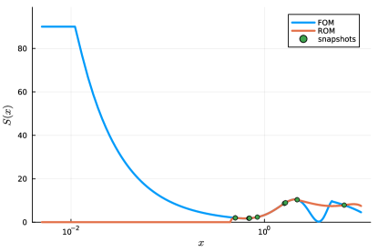
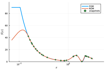
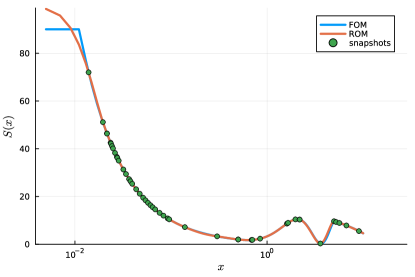
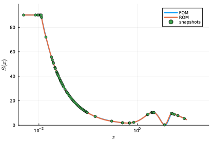
Fig. 1: Illustration of the algorithm adaptive behavior (example 1). The four plots illustrate the algorithm at iteration $k=1,20,40,60$. They display in blue the score function $S^{\ast}$ (the rare event being $S^{\ast}(X)\geq 90$), in red the reduced score approximation $S^{(k)}$, in green the snapshots $(X_{1},\ldots,X_{k})$ used to build the reduced score.

5.1.1 Example #1: spline approximation of a closed-form score

In a first numerical experiment, we design a one-dimensional analytical toy model. Cubic spline data interpolation is used to build the surrogate $S(x)$ from the snapshots and the error bound is set to the absolute value of the true error $E(x)=|S(x)-S^{\ast}(x)|$.

Using spline interpolation is not recommended in practice, as it easily creates wide oscillations that can artificially create spurious high score areas that misleads the sampling routines. It is nonetheless an interesting benchmark for difficult situations where the surrogate modeling is sub-optimal.

The score function, depicted in Figure 1, is defined for $x\in\mathcal{X}=\mathbb{R}_{+}$ by

$$S^{\ast}(x)=\left\{\begin{aligned} l_{\max}\quad&\textrm{if}\quad x\leq 1/l_{\max}\\ 1/x+f(x)\quad&\textrm{else}\end{aligned}\right.,$$

where $f(x)=\alpha\left(\,{\rm l}{\rm l}_{x_{0}\leq x<x_{1}}\sin(x-x_{0})^{2}+\,{\rm l}{\rm l}_{x_{1}\leq x}(\sin(x_{1}-x_{0})^{2}-\beta(x-x_{1}))\right),$ given parameters $x_{1}>x_{0}>1/l_{\max}$ and $\alpha,\beta>0$. The reference distribution $\pi$ is a log-normal distribution such that $\ln(x)\sim\mathcal{N}(1.5,1.5)$. The parameter are set to $x_{0}=0.5$, $x_{1}=5$, $\alpha=15$, $\beta=0.1$ and $l_{\max}=90$, corresponding to the rare event probability (computed analytically) $p^{*}_{l_{\max}}=\pi(\,{\rm l}{\rm l}_{S^{\ast}>l_{\max}})=2.18e-8$.

The initial surrogate is built using the 10 snapshots drawn according to the reference density.

Figure 1 shows a typical evolution of the spline-based score approximation as well as the selected snapshots over the iterations of the algorithm.

5.1.2 Example #2: reduced basis approximation of a PDE score

In our second numerical experiment, the score function is defined as $S^{\ast}(x)=\|\Psi^{\ast}(x)\|_{\infty}$ with $\Psi^{\ast}(x)$ being the high-fidelity numerical approximation of the solution of a bi-dimensional PDE parametrized by a $4$-dimensional random vector $x=(x_{1}\cdots x_{4})^{\intercal}\in\mathcal{X}=\mathbb{R}_{+}^{4}$. The chosen PDE corresponds to the well-studied thermal block problem, which models heat diffusion in an heterogeneous media. The reference distribution for $x$ will be a log-normal distribution with independent components with $\ln(x_{q})\sim\mathcal{N}(1.5,1.5)$, for $q=1,\ldots,4$. The probability of interest will correspond to the occurrence of a temperature exceeding a given threshold $l_{\max}=3$ in some point of the spatial domain $\Omega=[0,1]^{2}$. The PDE solution will be approximated using the popular reduced basis (RB) method.

We begin by describing the parametric PDE and the high-fidelity numerical approximation of its solution. The temperature function $\Psi$ over $\Omega$ is ruled by the elliptic problem

$$\left\{\begin{aligned} -\nabla\cdot(\kappa(\cdot;x)\nabla\Psi)=&1\quad\textrm{in}\quad\Omega\\ \Psi=&0\quad\textrm{on}\quad\partial\Omega\end{aligned}\right.,$$

where the function $\kappa(\cdot;x):\Omega\to\mathbb{R}_{+}$ represents a parametric diffusion coefficient function.

The high-fidelity approximation $\Psi^{\ast}(x)$ of the solution of this diffusion problem entails the solution of a variational problem. Precisely, let $\mathcal{V}$ denote the Hilbert space $\mathcal{H}^{1}_{0}(\Omega)$ and $\|\cdot\|_{\mathcal{V}}$ the norm induced by the inner product defined over $\mathcal{V}$. For any $x\in\mathcal{X}$, we define the solution $\Psi^{\star}(x)\in\mathcal{V}$ of the variational problem $a(\Psi(x),\nu;x)=\int_{\Omega}\nu\mathrm{d}\Omega,\quad\forall\nu\in\mathcal{V},$ where $a:\mathcal{V}\times\mathcal{V}\to\mathbb{R}$ is the bilinear form $a(u,\nu;x)=\int_{\Omega}\kappa(\cdot;x)\nabla u\cdot\nabla\nu d\Omega$. We consider the piecewise constant diffusion coefficient $\kappa(\cdot;x)=\sum_{q=1}^{4}\,{\rm l}{\rm l}_{z\in\Omega_{q}}(\cdot)x_{q}$ with the partition $\Omega=\cup_{q=1}^{4}\Omega_{q}$ and $\Omega_{q}$’s being non-overlapping squares. Setting the parameter space $\mathcal{X}=(\mathbb{R}_{+})^{4}$ implies that the bilinear form is strongly coercive, and the Lax-Milgram lemma ensures the variational problem has a unique solution.

Consider next a finite $h$-dimensional subspace $\mathcal{V}_{h}\subset\mathcal{V}$. The high-fidelity approximation $\Psi^{\ast}(x)\in\mathcal{V}_{h}$ of the solution $\Psi^{\star}(x)$ is defined for any $x\in\mathcal{X}$ by

$$\Psi^{\ast}(x)=\arg\min_{\nu\in\mathcal{V}_{h}}\|\Psi^{\star}(x)-\nu\|^{2},$$

with the energy norm induced by the bilinear form $\|\nu\|=\sqrt{a(\nu,\nu;x)}$. The high-fidelity approximation $\Psi^{\ast}(x)$ is obtained in practice by solving a large system of $h$ linear equations. [21]

We perform standard AMS computations with a score based on this high-fidelity approximation $\Psi^{\ast}(x)$ and using $N=900$ particles. By averaging over 10 runs, we obtain after an extremely intensive calculation an empirical approximation reference of the sought rare event probability $p^{*}_{l_{\max}}=\pi(\,{\rm l}{\rm l}_{S^{\ast}>l_{\max}})\approx 1.47e-04$.

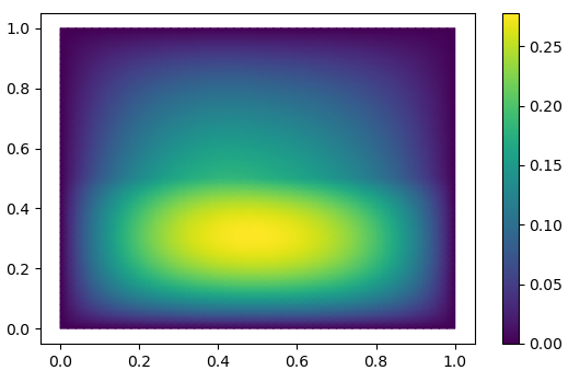
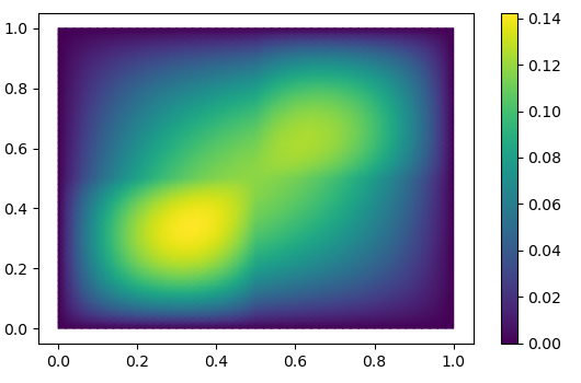
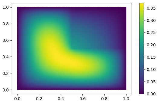
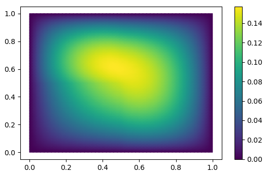
Fig. 2: Illustration of the thermal block problem (example 2). High-fidelity solution $\Psi^{\ast}(X)$ of the PDE for $4$ different samples $X$ of the reference log-normal distribution.

We are interested in the construction of an inexpensive approximation to the set of high-fidelity solutions

$$\mathcal{M}=\{\Psi^{\ast}(x)\in\mathcal{V}_{h}:x\in\mathcal{X}\},$$

by evaluating only some of its elements. By selecting a well-chosen set of $K$ snapshots $\{\Psi^{\ast}(x_{i})\}_{i=1}^{K}$, the RB framework approximates $\mathcal{M}$ in a well-chosen linear subspace $\mathcal{V}_{K}\subset\mathcal{V}_{h}$ of much lower dimension $K\ll h$. Using this framework yields i) an approximation $\Psi$ of the high-fidelity solution $\Psi^{\ast}$ which is used to compute the approximation $S(x)=\|\Psi(x)\|_{\infty}$ of the score $S^{\star}(x)$, ii) a so-called a posteriori error bound $E(x)$ which satisfies $|S^{\ast}(x)-S(x)|\leq\|\Psi^{\ast}(x)-\Psi(x)\|_{\mathcal{V}_{h}}\leq E(x)$. The high-fidelity solution, the RB approximation and the a posteriori error bounds are computed via the “pymor” Python^® toolbox [18] available at https://github.com/pymor/pymor. Figure 2 shows several $\Psi^{\ast}(x)$ solutions for samples drawn according to the reference distribution.

Let us comment on two important features of the RB approximation in regards to our rare event simulation framework. First, we emphasize that our algorithm enriches the RB approximation space using a variant of the popular week greedy algorithm. Indeed, the latter selects at each iteration the snapshot in the solution set $\mathcal{M}$ which possess the worst a posterior error bound for the current RB approximation. This setting is used in our snapshot selection in the first stage of the algorithm, i.e., in the case where the learning function selects the parameter maximizing the error. It should be noted, however, that snapshot selection differs in the second stage of our algorithm, in which the RB is enriched with a sample drawn according to the importance distribution.

Second, as in standard RB approaches, we here extensively rely on the affine parametric dependence of the RB approximation by splitting the assembly of the reduced matrices and vectors in an off-line and on-line phases. The former, which is performed once for all at each RB update, entails the computation of all the $h$-dependent and $x$-independent structures. It requires $\mathcal{O}(Kh^{2}+K^{2}h)$ operations. Besides, one must add the evaluation of a snapshot per se, which is $\mathcal{O}(h^{3})$. In the latter, on-line phase, for a given parameter $x\in\mathcal{X}$, we assemble and solve the RB system and provide the error bound in $\mathcal{O}(K^{3})$, with a cost depending only on $K$. For further details, we refer the reader to the introductory book on RB [21].

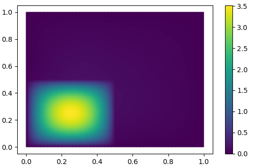
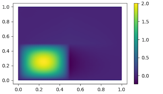
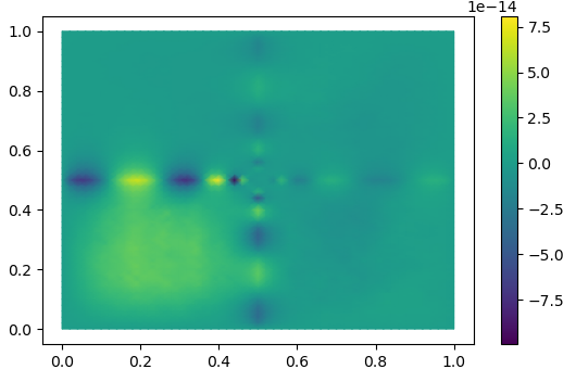
Fig. 3: Illustration of RB approximations of a rare event (example 2). The figure displays on the left the high-fidelity solution $\Psi^{\ast}(X)$ of the PDE for a parameter $X$ sampled according to the distribution $\propto\,{\rm l}{\rm l}_{S^{\star}>l_{\max}}d\pi$ (simulated by our ARMS algorithm). Images on the right are RB approximation errors related to $S^{(1)}$ and $S^{(K)}$, the initial and final reduced score approximations.

Figure 3 illustrates a high-fidelity approximation related to the rare event (i.e., $S^{\star}(x)>l_{\max}$) obtained by our algorithm. The figure also shows that the initial RB approximation is insufficiently accurate to discriminate this rare event (i.e., $S(x)<l_{\max}$), while at the end of the algorithm the RB approximation is almost indistinguishable from the high-fidelity one.

5.2 Results

We begin by detailing the experimental setup for evaluation. Our numerical simulations were carried out using an implementation of the ARMS algorithm in the Julia language, available at https://gitlab.inria.fr/pheas/arms. ARMS is configured as follows: a mutation proposal based on an Ornstein-Uhlenbeck [14] adaptive state movement, a number of particles $N$ is set by default to $1e3$ and $1e2$ in the first and second examples respectively and explicitly given otherwise, a quantile $\theta=0.3$ (i.e., a maximum number of kills in the selection steps of $M=0.3*N$), the number of hits of the rare event is $J=5$, the number of Markov transitions at each mutation step is set to $1e2$ and $3e1$ in the first and second examples respectively.

We compute $R$ independent ARMS runs and plot the median and quantiles related to the IS estimate $\hat{p}_{l_{\max}}^{H,N}$ and to the AMS estimate $\hat{p}_{l_{\max}}^{N}$ as a function of the number of snapshots $k$. ARMS performance is quantified by evaluating the expected cost as a function of the relative root expected square error. More specifically, after $k$ snapshots, the relative root expected square error is approximated over runs by the empirical average

$$\frac{\sqrt{\mathbb{E}(\hat{p}_{l_{\max}}^{H,N}-p^{*}_{l_{\max}})^{2}}}{{p^{*}_{l_{\max}}}}\approx\left(\frac{1}{R}\sum_{i=1}^{R}\frac{(\hat{p}_{l_{\max},i}^{H_{k},N}-{p^{*}_{l_{\max}})}^{2}}{{p^{*}_{l_{\max}}}^{2}}\right)^{1/2},$$ (5.1)

where $\hat{p}_{l_{\max},i}^{H_{k},N}$ denotes, at the $i$-th run and after $k$ snapshots, the importance sampling estimate $\hat{p}_{l_{\max},i}^{H_{k},N}$ if $H_{k}:=k-K_{\min}>0$ and $\hat{p}_{l_{\max},i}^{H_{k},N}=0$ otherwise. After $k$ snapshots, the expected cost (in units of the cost of evaluating $S^{\ast}$) is approximated over the runs by the empirical average

$$\textrm{cost(k)}\simeq k+\frac{1}{R}\sum_{i=1,k^{\prime}=1}^{R,k}N^{(k^{\prime})}_{i}\textrm{gain}^{(k^{\prime})}$$ (5.2)

with $\textrm{gain}^{(k^{\prime})}$ representing the ratio of the cost of evaluating the reduced score $S^{(k^{\prime})}$ to the cost of the true score $S^{\ast}$, and where $N^{(k^{\prime})}_{i}$ represents the number of evaluations of the reduced score at the $k^{\prime}$-th iteration and $i$-th execution of the ARMS algorithm.

Please note that for the first example, $\textrm{gain}^{(k^{\prime})}$ will be set artificially smaller to emulate more realistic cases in which the cost of evaluating the surrogate is indeed cheaper than that of the true model (see Figure 5).

We will compare the performance of ARMS with the empirical average of the estimates obtained by performing $R$ standard AMS with the true score $S^{\ast}$ with a number of particles $N$ in the range $[1e2,1e4]$.

5.2.1 Example #1

$e=42*e_{\min}$	$e=e_{\min}$
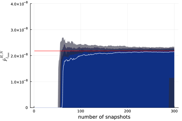
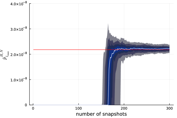
$e=28*e_{\min}$

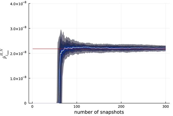
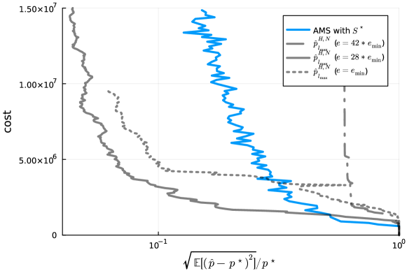
Fig. 4: Influence of the entropic criterion threshold $e$ (example 1). Upper and lower left plots: median (in white) and quantiles (in shades of blue-grey) related to the IS estimate (4.10) as a function of the number of snapshots (equal to the number of iteration $k$ of the algorithm) for $3$ different values of the worst log cost threshold $e$. The red line denotes the true rare event probability. Lower right plot: expected cost (5.2) as a function of the relative root expected square error (5.1) (grey curves). Comparison to the performance of standard AMS with $S^{\ast}$ and $N\in[1e2,1e4]$ (blue curve).

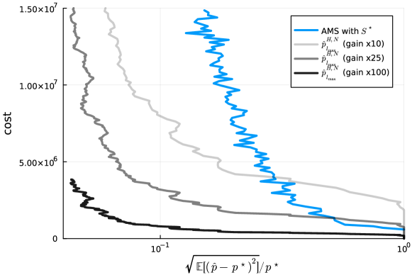
Fig. 5: Performance with respect to the reduced score gain (example 1). Expected cost (5.2) as a function of the relative expected squared error (5.1) for different values of the ratio between the cost of evaluating $S^{(k)}$ and $S^{\ast}$ (grey curves) and for the threshold $e=28e_{\min}$. Comparison to the performance of standard AMS with $S^{\ast}$ and $N\in[1e2,1e4]$ (blue curve).

no bridge, $\epsilon=0$, $N=1e3$	bridge, $\epsilon=0$, $N=1e3$
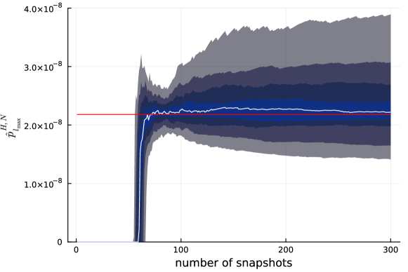
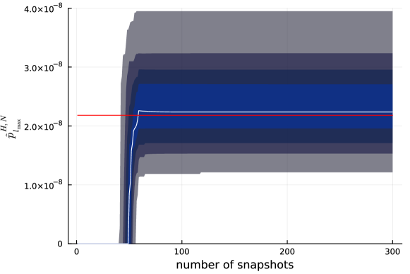
bridge, $\epsilon=0$, $N=2e4$

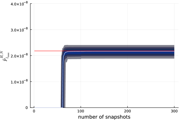
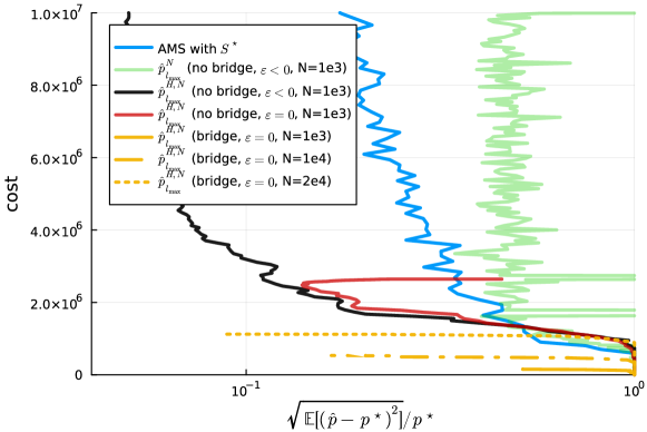
Fig. 6: Bridging performance (example 1). Upper and lower left plots: median (in white) and quantiles (in shades of blue-grey) related to the IS estimate (4.10) as a function of the number of snapshots for $3$ different setups (update stopping criterion $\epsilon$, bridging simulation or not, number of samples $N$). Entropic criterion set to $e=28*e_{\mathrm{min}}$ and gain between surrogate and exact is assumed to be $25$. The red line denotes the true rare event probability. Lower right plot: expected cost (5.2) as a function of the relative root expected square error (5.1) for the various setups. Comparison to the performance of standard AMS with $S^{\ast}$ and $N\in[1e2,1e4]$ (blue curve) and to the performance of the reduced-based estimate (4.12) (green curve).

We perform $R=100$ runs of the ARMS algorithm, each one of them targeting $p_{l_{\max}}^{\ast}\approx 2.2e-8$ with a budget of $K=300$ snapshot evaluations.

Figure 4 evaluates the influence of the threshold $e$ on the entropic criterion of Section 2.2. The three quantiles show the distribution of the IS estimate as a function of the number of snapshots for different values of the entropy criterion threshold $e$. As expected, we note that too high, a threshold produces over 40% of erroneous IS estimates, associated with zero probability regardless of the number of reduced score updates. Although the remaining 60% of estimates nevertheless become accurate after around 60 updates of the reduced score, this demonstrates that increasing the critical level too quickly tends to concentrate particles around unimportant local minima. This results in sampling snapshots and refining the reduced score exclusively in regions of state space unrelated to the rare event of interest. To avoid this undesirable scenario, it is prudent to set the threshold to its minimum value $e_{\min}$, which has the disadvantage of delaying the convergence of the IS estimate. Indeed, the plot shows convergence of all estimates towards a non-zero value close to $p_{l_{\max}}^{\ast}$, but with a considerable delay, since in this case about a hundred more updates of the reduced score are required. A well-tuned value between these extrema achieves convergence after about 70 snapshots, with a characterization of the distribution of IS estimates comparable to the safe distribution obtained with the minimum value.

This trend is confirmed by plotting the expected cost (5.2) as a function of the relative root expected square error (5.1). In the case of a not-too-high threshold $e$, given a certain precision (i.e., after sampling enough snapshots), we observe a gain in expected cost from around a decade onwards, which increases more and more. Clearly, too high a value for $e$ do not achieve comparable accuracy, regardless of the number of snapshots.

Figure 5 illustrates how the gain in terms of expected cost over accuracy can be dramatic, as the cost of evaluating $S^{(k)}$ becomes negligible compared to $S^{\ast}$.

The evaluation above focused on the ARMS algorithm in which the simulation is restarted after each snapshot update and the reduced score update stop criterion introduced in Section 2.5 is never triggered ($\epsilon<0$). Figure 6 extends the analysis by evaluating the influence of activating the stop update criterion ($\epsilon\geq 0$) and of bridging the simulations between two iterations, as presented in Section 4.3. The entropic criterion set to $e=28*e_{\mathrm{min}}$. Reference to exact AMS cost is made with a cost gain between surrogate and exact of $25$.

Plotting the predicted cost versus accuracy in the lower right box of Figure 6 shows the considerable savings brought by the bridging procedure.

Some additional remarks on Figure 6 are required.

First, one can remark that, when using the bridging procedure, and for a given sample size, we cannot expect better accuracy for the IS estimator $p_{l_{\max}}^{H,N}$ than for $\hat{p}^{N}_{l_{\max}}$ as both estimates (4.11) and (4.12) depend on the variance of the normalization constant ${Z_{l^{(k)}}^{N,(k)}}$. However, as the same figure shows, because the bridging procedure offers a significant cost saving, we can afford to gain in precision by increasing the number of samples $N$: the curves in yellow in the lower right plot of Figure 6 do show that we obtain a more accurate IS estimate (lower variance and a smaller apparent bias) for a given computational cost.

On the other hand, we notice that enabling the stop-update criterion, even without bridging, induces a spread around the mean of the distribution of the IS estimate in the upper left plot of Figure 6. This expresses (as will show a close look at the expected cost versus accuracy red curve in the lower right plot) the fact that the IS estimator in fact again achieves the accuracy of the reduced score based estimate $p_{l_{\max}}^{N}$ given in (4.12). This latter fact is a consequence of freezing the estimate ${Z_{l^{(k)}}^{N,(k)}}$ as soon as the stop-update criterion is activated and using the latter until the snapshot budget is exhausted. As a result, the variance of the lastest computed normalization constant will affect our IS estimate. The phenomenon does not appear when the stop-update criteria is off (Figure 4) and we restart the simulation as before and calculate a new normalization constant at each iteration (at each iteration). The stop-update criteria is, in fact, simply used to marginally reduce the cost in the bridging procedure, without changing the outcome (not shown in plot).

5.2.2 Example #2

no bridge, $\epsilon=0$, $N=1e2$	bridge, $\epsilon=0$, $N=1e2$
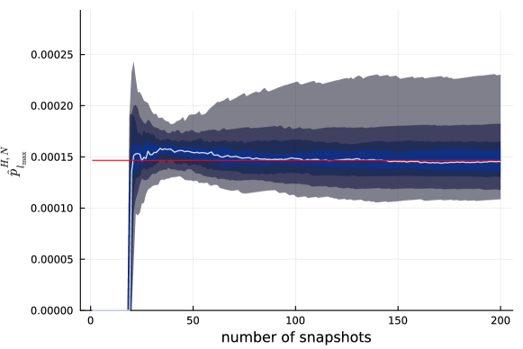
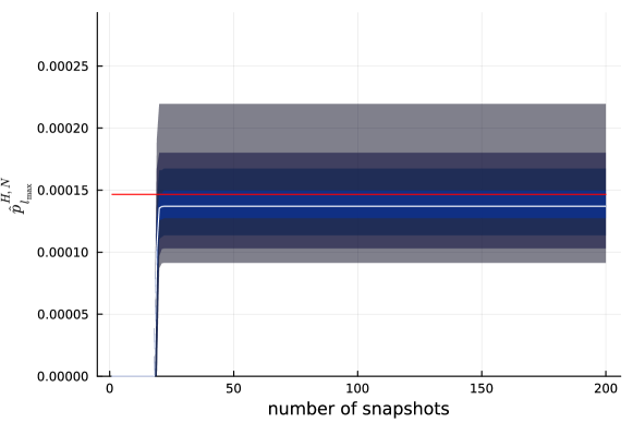
bridge, $\epsilon=0$, $N=4e3$

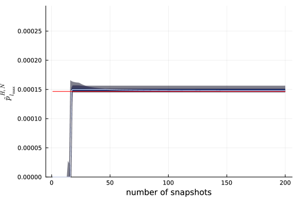
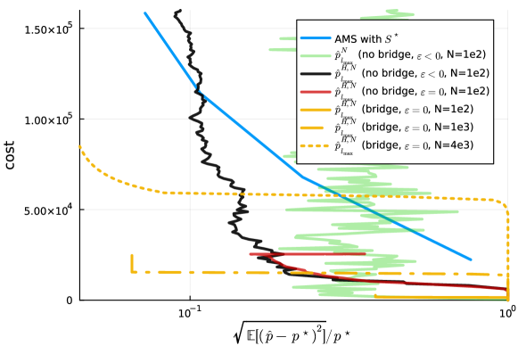
Fig. 7: Performance evaluation (example 2). Upper and lower left plots: median (in white) and quantiles (in shades of blue-grey) related to the IS estimate (4.10) as a function of the number of snapshots for $3$ different setups (update stopping criterion $\epsilon$, bridging simulation or not, number of samples $N$). The red line denotes the true rare event probability. Lower right plot: expected cost (5.2) as a function of the relative root expected square error (5.1) for the various setups. Comparison to the performance of standard AMS with $S^{\ast}$ and $N\in[1e2,2e3]$ (blue curve) and to the performance of the reduced-based estimate (4.12) (green curve).

We perform $R=100$ runs of the ARMS algorithm, each one of them targeting $p_{l_{\max}}^{\ast}\approx 1.5e-4$ with a budget of $K=200$ snapshot evaluations. We set the worst log cost threshold to $e=35\,e_{\min}\approx 0.5$. Overall, the trends of the algorithm for this RB approximation of a PDE score are similar to those of the previous example. Below, we comment on some of the remarkable results.

We analyze in Figure 7 performances using an initial reduced score built on a $5$-dimensional RB approximation. The curves show that about $10$ to $20$ more snapshots are needed to reach convergence, with a median estimate around $p_{l_{\max}}^{\ast}$.

In the case where simulations are not bridged (but we stop updating the reduced score once the worst-case log cost has reached $\epsilon=0$), the distribution of the IS estimate converges after about $50$ more iterations, with some variance but no bias. In the case of bridging, we observe that the distribution of the IS estimate jumps to a constant distribution, with a similar variance but a slight bias. With regard to the latter remark, we suspect that, although the bridging procedure considerably reduces the cost (compared to restarting the simulation in the first iterations of the algorithm), it nevertheless leads to a larger variance of the normalization constant and thus to an apparent bias in the IS estimate. The first remark is simply explained by the fact that the bridging procedure adapts the level for the next iteration of the algorithm to a level so close to $l_{\max}$ that all snapshots are sampled in the rare event, which induces an IS estimate exactly equal to the estimate of the normalization constant ${Z_{l^{(k)}}^{N,(k)}}$.

However, as before, increasing the number of samples $N$ when using bridging yields a reduction of the variance and of the apparent bias while preserving a low expected cost, as shown in the quantile plots and the curves of expected cost versus accuracy in Figure 7.

6 Conclusions and Perspectives

This work proposes an adaptive algorithm called ARMS that reduces the cost of AMS simulation when the score function $S^{\ast}$ is very expensive to compute.

The general idea of ARMS is to perform iterative importance sampling of a sequence of target distributions of the form $\propto\,{\rm l}{\rm l}_{{S^{\ast}}>l^{(k)}}d\pi$ parametrized at iteration $k$ by the level $l^{(k)}\in\mathbb{R}$, using a sequences of proposals of the form $\mu_{l^{(k)}}^{(k)}\propto\,{\rm l}{\rm l}_{{S^{(k)}}>l^{(k)}}d\pi$, much cheaper to simulate with AMS. As the algorithm is iterated, the proposals are adapted by adjusting the level $l^{(k)}$ and refining the approximation of the reduced score $S^{(k)}$ using the history of score evaluations previously calculated for importance sampling.

As $S^{(k)}$ gains in accuracy and $l^{(k)}$ increases, the reduced score approximation should be refined using samples of the state space in regions closer and closer to the rare event of interest. However, an essential ingredient in achieving this desirable convergence is to determine a heuristic for setting the first non-achievable level $l^{(k)}$ suitable for the accuracy of the current reduced score approximation $S^{(k)}$. In addition, one of the conditions of importance sampling is to ensure that the proposal dominates the target. Justified by theoretical arguments, these two problems are addressed in ARMS using entropy constraints: $l^{(k)}$ is chosen such that $i)$ the relative entropy between a pessimistic target and the proposal corresponds to a given logarithmic cost of importance sampling; $ii)$ the relative entropy between an optimistic target and the proposal remains finite. Pessimistic and optimistic targets are constructed using a quantification of the worst-case error associated with the reduced score approximation.

A final point addressed by ARMS is the adaptation of the proposal to a new approximation of the reduced score $S^{(k+1)}$. In particular, the algorithm ensures that the updated proposal dominates a well-chosen previous proposal, so that the two proposals can be bridged in a single AMS simulation step. To achieve this, ARMS searches among past simulation indexes $k_{bridge}<k+1$ for an approximation $S^{(k_{bridge})}$ and an initial level $l_{bridge}(k+1)$ such that $iii)$ the relative entropy between the new proposal $\mu_{l_{\mathrm{bridge}}(k+1)}^{(k+1)}$ at its initial level and the past proposal ${\mu_{l^{(k_{\mathrm{bridge}})}}^{(k_{\mathrm{bridge}})}}$ at its final level is kept below a certain standard AMS threshold and, in addition, such that both entropy constraints $i)$ and $ii)$ are satisfied.

In addition to demonstrating the unbiasedness of our estimator in an idealized setting, we evaluate in our numerical experiments the empirical convergence of the ARMS algorithm on a toy model and a rare-event problem based on a more realistic PDE. Our study confirms that entropy criteria play a crucial role in ARMS. In particular, as expected, too high a value of the logarithm of the cost in the entropy criterion $i)$ can take ARMS into spurious regions of the state-space remote from the region of interest, resulting in a large variance of the IS estimator. Too small a value gives a more desirable variance but a slower rate of convergence. We show empirically that the approximation procedure using the entropy criterion $iii)$ significantly reduces simulation cost while achieving a comparable squared error.

The prospects arising from this work are numerous. These include answering open theoretical questions, including the consistency of ARMS, which is proven in the present paper only in a formal sense. No straightforward answers seem available, as we are confronted with a non-standard framework in which interacting particles in AMS simulations have distributions with varying supports which depend on random approximations of the reduced score. Future research directions also include extending ARMS to smooth proposal distributions, with the advantage of removing nesting and domination constraints, or particularizing this approach to the simulation of rare events driven by stochastic dynamics.

Appendix A Sample Size for Importance Sampling

A.1 Generic quantification rules

Importance sampling of some generic distribution $\eta\propto\gamma$ known up to a normalizing constant $p=\gamma(\,{\rm l}{\rm l})$ using a proposal distribution $\mu$ is based on the following identity

$$\gamma(\varphi)=p\,\eta(\varphi)=\mathbb{E}_{\mu}\left[f(X)\varphi(X)\right]\qquad\forall\varphi:\mathcal{X}\to\mathbb{R}$$

where $f(x)=\frac{d\gamma}{d\mu}(x)$ is computable in closed-form.

Unfortunately, importance sampling becomes quickly infeasible if the target distribution diverges too widely from the proposal, a typical phenomenon in high dimension. This can be readily seen by computing the relative variance of the importance sampling estimator for $\varphi=\,{\rm l}{\rm l}$:

$$\operatorname{\mathbb{V}ar}_{\mu}(f(X))/p^{2}=\eta(\frac{\mathrm{d}\eta}{\mathrm{d}\mu})-1=\mathrm{e}^{\mathrm{Ent}_{2}(\eta\mid\mu)}-1,$$

where we have denoted $\mathrm{Ent}_{2}(\eta\mid\mu)=\ln\eta(\frac{\mathrm{d}\eta}{\mathrm{d}\mu})$ the order $2$ Rényi entropy (also known as $\chi^{2}$-divergence). The latter scales linearly in $d$ if $\mu$ and $\eta$ are a $d$-fold product measure, generating a variance exponential with $d$.

As is thoroughly argued in [7] (see also [6]), the variance ($e^{\mathrm{Ent}_{2}(\eta\mid\mu)}-1$) is in general a pessimistic quantification of importance sampling, whose cost is better estimated using a $\mathbb{L}^{1}$-error, or a success probability within a tolerance precision. For a target $\eta$ with proposal $\mu$, it has been proven in  [7] that the cost of importance sampling – in terms of sample size $K$– is roughly given (up to a reasonable tail condition on the log-density $\ln\frac{\mathrm{d}\eta}{\mathrm{d}\mu}$), by the exponential of the relative entropy between $\eta$ and $\mu$:

$$K\simeq\mathrm{e}^{\mathrm{Ent}(\eta\mid\mu)}.$$

Remark A.1.

Jensen inequality

$$\mathrm{Ent}_{2}(\eta\mid\mu)=\ln\eta(\frac{\eta}{\mu})\geq\eta(\ln\frac{\eta}{\mu})=\mathrm{Ent}(\eta\mid\mu),$$

shows that indeed, variance is (in general) not a sharp estimate of the required sample size for importance sampling.

A.2 Particular case of interest

We will particularize the above discussion to the family of distributions studied in our paper: distributions of propositions of the form $\mu\propto\,{\rm l}{\rm l}_{B}d\pi$ and a target $\eta\propto\,{\rm l}{\rm l}_{A}d\pi$ such that $A\subseteq B$.

In accordance with the importance sampling identity, the normalization $p$ is estimated without bias using the random variable $f(X)=\pi(B)\,{\rm l}{\rm l}_{A}(X)$ where $X\sim\mu$.

In this remarkable case, it turns out that the relative variance and the exponential of the relative entropy reduces to the same quantity. In other words, we reach the limit of Jensen’s inequality in the Remark A.1

$$\mathrm{Ent}_{2}(\eta\mid\mu)=\mathrm{Ent}(\eta\mid\mu)=\ln\frac{\pi(B)}{\pi(A)}.$$

Therefore, in our study, we will refer indifferently to the exponential of the relative entropy $e^{\mathrm{Ent}(\eta\mid\mu)}$ or to the relative variance $e^{\mathrm{Ent}_{2}(\eta\mid\mu)}$ to designate the importance sampling cost of the target $\eta$ by the proposal $\mu$.

Appendix B Consistency of the Estimator

For simplicity (but the general case is similar), we restrict to the case where $\tau^{(k)}=0$ for $k\geq K_{\mathrm{min}}+1$ in the estimator (3.1), as well as $\varphi=\,{\rm l}{\rm l}$. We thus consider the rare event probability estimator: $\hat{p}_{l}^{H}=\hat{\gamma}^{H}_{l}(\,{\rm l}{\rm l}).$

Proposition B.1.

The estimator $\hat{p}_{l}^{H}$ is unbiased, i.e., $\mathbb{E}\,\hat{p}_{l}^{H}=p_{l}^{\ast},$ and its relative variance is given by

$$\operatorname{\mathbb{V}ar}\left[\hat{p}_{l}^{H}\right]/{p^{\ast}_{l}}^{2}=\frac{1}{H^{2}}\sum_{k=K_{\mathrm{min}}+1}^{K_{\mathrm{min}}+H}\left(\frac{\pi(\,{\rm l}{\rm l}_{S^{(k)}>l^{(k)}})}{p^{\ast}_{l}}-1\right).$$ (B.1)

Proof.

We first show that the random sequence

$$H\mapsto M_{H}\displaystyle\mathop{=}^{{\rm def}}H\,(\hat{\gamma}_{l}^{H}-\gamma^{\ast}_{l}),$$

is a martingale with respect to the filtration generated by the snapshots. Indeed, it follows from the definition (3.1) that

$$\mathbb{E}[M_{H}|X_{1},\ldots,X_{H}] =\mathbb{E}[\sum_{k^{\prime}=K_{\mathrm{min}}+1}^{K_{\mathrm{min}}+H}f_{l}^{(k^{\prime})}(X_{k^{\prime}+1})\delta_{X_{k^{\prime}+1}}-h\gamma^{\ast}_{l}|X_{1},\ldots,X_{H}],$$

$$=M_{H-1}+\mathbb{E}[f_{l}^{(\tilde{k})}(X_{\tilde{k}+1})\delta_{X_{\tilde{k}+1}}-\gamma^{\ast}_{l}|X_{1},\ldots,X_{H}],$$

$$=M_{H-1}+\pi(\,{\rm l}{\rm l}_{S^{\ast}>l})-\gamma^{\ast}_{l}=M_{H-1},$$

where $\tilde{k}={K_{\mathrm{min}}+H}$.

Now, since $M_{H}$ is a martingale, the estimators are unbiased $\mathbb{E}\,\hat{\gamma}_{l}^{H}=\gamma_{l}^{\ast},$ and their variances are given by the average of their quadratic variation. In particular, the variance is for the rare event probability estimator

$$H^{2}\operatorname{\mathbb{V}ar}\left[\hat{p}_{l}^{H}\right] ={p^{\ast}_{l}}^{2}\sum_{k=K_{\mathrm{min}}+1}^{K_{\mathrm{min}}+H}\left(\mathrm{e}^{\mathrm{Ent}_{2}\left(\eta_{l}^{\ast}\mid\mu^{(k)}_{l^{(k)}}\right)}-1\right),$$

which particularizes for $\eta_{l}^{\ast}\propto\,{\rm l}{\rm l}_{S^{\ast}>l}d\pi$ and $\mu^{(k)}_{l^{(k)}}\propto\,{\rm l}{\rm l}_{S^{(k)}>l^{(k)}}d\pi$ to (B.1).$\quad\square$

References

- [1] Siu-Kui Au and James L Beck. Estimation of small failure probabilities in high dimensions by subset simulation. Probabilistic engineering mechanics, 16(4):263–277, 2001.
- [2] Mathieu Balesdent, Jerome Morio, and Julien Marzat. Kriging-based adaptive importance sampling algorithms for rare event estimation. Structural Safety, 44:1–10, 2013.
- [3] Julien Bect, Ling Li, and Emmanuel Vazquez. Bayesian subset simulation. SIAM/ASA Journal on Uncertainty Quantification, 5(1):762–786, 2017.
- [4] Claire Cannamela, Josselin Garnier, and Bertrand Iooss. Controlled stratification for quantile estimation. The Annals of Applied Statistics, 2(4):1554–1580, 2008.
- [5] Frédéric Cérou and Arnaud Guyader. Fluctuation analysis of adaptive multilevel splitting. Annals of Applied Probability, 26(6):3319–3380, December 2016.
- [6] Frédéric Cérou, Patrick Héas, and Mathias Rousset. Entropy minimizing distributions are worst-case optimal importance proposals. arXiv preprint arXiv:2212.04292, 2022.
- [7] Sourav Chatterjee and Persi Diaconis. The sample size required in importance sampling. The Annals of Applied Probability, 28(2):1099–1135, 2018.
- [8] Peng Chen and Alfio Quarteroni. Accurate and efficient evaluation of failure probability for partial different equations with random input data. Computer Methods in Applied Mechanics and Engineering, 267:233–260, 2013.
- [9] Pieter-Tjerk De Boer, Dirk P Kroese, Shie Mannor, and Reuven Y Rubinstein. A tutorial on the cross-entropy method. Annals of operations research, 134(1):19–67, 2005.
- [10] Pierre Del Moral, Arnaud Doucet, and Ajay Jasra. Sequential monte carlo samplers. Journal of the Royal Statistical Society Series B: Statistical Methodology, 68(3):411–436, 2006.
- [11] Benjamin Echard, Nicolas Gayton, and Maurice Lemaire. AK-MCS: an active learning reliability method combining kriging and monte carlo simulation. Structural Safety, 33(2):145–154, 2011.
- [12] Daniel Elfverson, Robert Scheichl, Simon Weissmann, and F Alejandro DiazDelaO. Adaptive multilevel subset simulation with selective refinement. arXiv preprint arXiv:2208.05392, 2022.
- [13] Laurent Gallimard. Adaptive reduced basis strategy for rare-event simulations. International Journal for Numerical Methods in Engineering, 120(3):283–302, 2019.
- [14] Paul H Garthwaite, Yanan Fan, and Scott A Sisson. Adaptive optimal scaling of metropolis–hastings algorithms using the robbins–monro process. Communications in Statistics-Theory and Methods, 45(17):5098–5111, 2016.
- [15] Patrick Héas. Selecting reduced models in the cross-entropy method. SIAM/ASA Journal on Uncertainty Quantification, 8(2):511–538, 2020.
- [16] Matthias Heinkenschloss, Boris Kramer, and Timur Takhtaganov. Adaptive reduced-order model construction for conditional value-at-risk estimation. SIAM/ASA Journal on Uncertainty Quantification, 8(2):668–692, 2020.
- [17] Chunyan Ling, Zhenzhou Lu, Kaixuan Feng, and Xiaobo Zhang. A coupled subset simulation and active learning kriging reliability analysis method for rare failure events. Structural and Multidisciplinary Optimization, 60(6):2325–2341, 2019.
- [18] René Milk, Stephan Rave, and Felix Schindler. pymor–generic algorithms and interfaces for model order reduction. SIAM Journal on Scientific Computing, 38(5):S194–S216, 2016.
- [19] Maliki Moustapha, Stefano Marelli, and Bruno Sudret. Active learning for structural reliability: Survey, general framework and benchmark. Structural Safety, 96:102174, 2022.
- [20] Benjamin Peherstorfer, Karen Willcox, and Max Gunzburger. Survey of multifidelity methods in uncertainty propagation, inference, and optimization. Siam Review, 60(3):550–591, 2018.
- [21] Alfio Quarteroni, Andrea Manzoni, and Federico Negri. Reduced basis methods for partial differential equations: an introduction, volume 92. Springer, 2015.
- [22] Nassim Razaaly, Daan Crommelin, and Pietro Marco Congedo. Efficient estimation of extreme quantiles using adaptive kriging and importance sampling. International Journal for Numerical Methods in Engineering, 121(9):2086–2105, 2020.
- [23] Felipe Uribe, Iason Papaioannou, Youssef M Marzouk, and Daniel Straub. Cross-entropy-based importance sampling with failure-informed dimension reduction for rare event simulation. SIAM/ASA Journal on Uncertainty Quantification, 9(2):818–847, 2021.
- [24] Fabian Wagner, Jonas Latz, Iason Papaioannou, and Elisabeth Ullmann. Multilevel sequential importance sampling for rare event estimation. SIAM Journal on Scientific Computing, 42(4):A2062–A2087, 2020.
- [25] Jize Zhang and Alexandros A Taflanidis. Adaptive kriging stochastic sampling and density approximation and its application to rare-event estimation. ASCE-ASME Journal of Risk and Uncertainty in Engineering Systems, Part A: Civil Engineering, 4(3):04018021, 2018.