Sample selection with noise rate estimation in noise learning of medical image analysis

Abstract

Deep learning techniques have demonstrated remarkable success in the field of medical image analysis. However, the existence of label noise within data significantly hampers its performance. In this paper, we introduce a novel noise-robust learning method which integrates noise rate estimation into sample selection approaches for handling noisy datasets. We first estimate the noise rate of a dataset with Linear Regression based on the distribution of loss values. Then, potentially noisy samples are excluded based on this estimated noise rate, and sparse regularization is further employed to improve the robustness of our deep learning model.
Our proposed method is evaluated on five benchmark medical image classification datasets, including two datasets featuring 3D medical images. Experiments show that our method outperforms other existing noise-robust learning methods, especially when noise rate is very big.
Key words: noise-robust learning, medical image analysis, noise rate estimation, sample selection, sparse regularization

1 Introduction

Deep learning has been widely used in medical image analysis tasks and achieved remarkable success. Its efficacy has been evidenced across diverse medical image analysis tasks, including regression (e.g. prediction children bone age with wrist joint X-ray), classification (whether there is pneumonia or not), detection (finding lung nodules), segmentation (segmenting brain haemorrhage regions) and text generation (generating radiological reports).
Despite the current success, challenges still exist with label noise emerging as a notable issue. ‘Label noise’ refers to the incorrect labels caused by various reasons, especially by the mistake of labellers. In deep learning-based image analysis, the availability of substantial quantities of accurately labeled images is imperative for the neural network to effectively learn and enhance its performance. Noisy labels hurt this process because neural network models might overfit to label noise, leading to the corrupted feature extractors.
Label noise is a common problem in deep learning, but it is even more severe in the domain of medical image analysis mainly for two reasons. The first reason is the difficulty and high consumption to label medical images. Analysing medical images requires expertise of medical imaging knowledge and experience, which is expensive to acquire. Furthermore, the privacy constraints of patient data made it difficult to collect large amounts of medical image datasets. The second reason is the inherent diagnostic limitations of medical images. Some types of medical images naturally can not provide an absolutely precise representation of the actual physiological conditions within the human body. Consequently, even if the labeller did a perfect job, the presence of label noise in medical image labels remains unavoidable. Additionally, severe inter-observer variability among experts [4][15] further compounds this issue, which means that top experts could have different interpretations of the same image and the potential for different labels.
Many studies have proved that noisy labels have negative impact on the performance of neural network models [19][1]. Various noise-robust learning methods have been proposed to address the issue of label noise, and many of them demonstrating efficacy in natural images. Some of these methods will be discussed in detail in the literature review. However, most of the existing noise-robust learning techniques still have not been used in medical images [14]. In this project, we aim to explore the efficacy of existing noise-robust methods in medical images and propose our original method. Our key contributions are summarized as follows:
i) We have introduced a three-phase learning scheme to filter clean data from a noisy medical image dataset. We have also incorporated GCE loss function and sparse regularization to further enhance its robustness.
ii) We have proposed a noise rate estimation module based on loss value distribution. Unlike previous works, our noise rate estimation module is based on linear regression. Our experiments have proved the accuracy of our linear regression model in predicting noise rates.
iii) We have implemented and compared our original method with various existing methods in medical images. Experimental results prove that our proposed method achieves superior performance in different kinds of medical images, including pathological slides, eye OCT images, X-ray, computed tomography (CT), and magnetic resonance imaging (MRI).
Specifically, to the best of our knowledge, our study stands as the first to validate the effectiveness of noise-robust deep learning algorithms on 3D medical images like CT and MRI.

2 Related work

2.1 General noise-robust learning methods

Many studies have been carried out to improve the noise robustness in natural image analysis, using different kinds of approaches. Some early studies modified the architecture of neural networks to make them work better on noisy datasets, mostly by add noise-adaption layers to the model. For example, Sukhbaatar [27] added an extra noise layer as part of the training process. which will adapt the network outputs to match the distribution of label noise.

Some other studies implemented noise-robust loss function or regularization methods specifically designed towards noisy datasets. Wang et al. [29] notice that cross entropy loss will easily overfit the false labels but have difficulty fitting hard correct labels. Inspired by symmetricity of Kullback-Leibler divergence, they combine CE loss with Reverse Cross Entropy and propose a more noise-robust loss function called Symmetric Cross Entropy. MixUp [39] is a commonly used regularization method by data augmentation that prevents overfitting. New data is formed simply by the linear interpolation of two training examples randomly chosen from the training dataset.

Noisy labels indicate false labels and lead to incorrection loss function and thus damage the parameter updating in backward propagation. So, correcting the labels and the loss value is another idea in noise-robust learning. Some studies try to build a transition matrix to correct the loss values. Patrini et al. [23] propose two procedures for estimating the transition matrix and correcting the loss, including ‘forward correction’ and ‘backward correction’. These two procedures are converse with each other but will improve the robustness to noise labels. Self-adaptive training [11] realizes that the prediction of DNN models exponents the useful information in the noisy data, so that using the prediction to refurbish the labels in training will be beneficial. This method also adopts sample reweighting strategy to tune the respective weights and improved the performance on noisy data. Interestingly, besides correcting the labels, some other studies remove the possibly noisy labels and transpose the noise learning problem to a semi-supervised learning problem. For example, DivideMix [20] uses two-component and one-dimensional Gaussian mixture models to transform noisy data into labeled (clean) and unlabeled (noisy) sets. Then, it applies a semi-supervised technique MixMatch [2].

2.2 Sample selection in natural image noise-robust learning

One simple and straightforward approach against label noise is finding the incorrectly labelled samples and removing them from the dataset. This procedure can be executed iteratively at each training epoch, or one time at certain stages during training. Some studies use multiple networks or multiple training stages to filter high-likely noisy data.
Decoupling [22] is an early method that uses more than one neural networks to select the possibly clean data. It created two networks which are maintained simultaneously. For every mini batch, only the samples that receive different predictions from the two networks were used to update the neural network parameters. This strategy is often referred to as ‘update by disagreement’. MentorNet [13] used a mentor network and a student network. The mentor network will find the small-loss samples and guide the training of student network by only feeding small-loss samples which are likely to be correctly labelled. Co-teaching [8] and Co-teaching+ [38] both maintained two networks. The two networks in Co-teaching will select samples with minimal losses and then feed them to its peer network. Co-teaching+ further integrated the ‘update by disagreement’ strategy from DeCoupling into Coteaching, thereby combining the strengths of both methods. Jo-SRC [30] also employed two networks, but adopted a contrastive learning approach. Predictions from two different views of each sample were used to estimate its likelihood of being clean or noisy. A joint loss function was proposed to improve the model generalization performance by using consistency regularization.
Some other studies use only one network, but implement multiple training rounds or phases to select clean data. In the method proposed by Shen et al. [25], during each training round, the model removed high-loss samples and the remaining small-loss samples were be used to train the network in the next round. O2U-Net [10] adopted three training stages. The first stage was pre-training, while in the second stage this pre-trained model was utilized to calculate the loss values of all samples and delete the high-loss data, creating a refined dataset. In the third stage, training restarted based on the cleaned dataset. MORPH [26] shared a similar idea with O2U, but this method was able to switch its learning phase at the transition point automatically. It also introduced the concept of memorized examples. Wu et al. [31] proposed a new data-selection method by constructing a nearest neighbour graph. Clean samples were identified by leveraging geometric structure of data and model predictive confidence. This method was effective not only on noisy labels, but also in handling out-of-distribution samples.
Chen et al. [6] integrated both multiple-networks and multiple-round approach. They randomly divided training data into different groups, and during each round they employed two networks in conjunction with cross-validation to classify correctly-labelled samples and remove high-loss samples that are likely to be incorrectly labelled.
It is evident that some of the these methods have trained multiple networks or conducted multiple training rounds, thereby spending much more time and resources in the training process.

2.3 Noise robust learning in medical image analysis

The study of Dgani et al. [7] was one of the earliest to apply noise robust deep learning techniques to medical images. They added a noise-robust layer to a neural network in a mammography classification task and slightly improved the accuracy. Pham et al. [24] used label smoothing techniques in the classification of chest X-ray images. By comparing their method with basic noise-robust methods, such as ignoring possibly noisy samples, they proved that label smoothing can achievement an improvement of up to 0.08 in AUC (area under curve) value. Xue et al. [34] presented a two-stage strategy for learning from corrupted skin lesion datasets. The first stage involved uncertainty sample mining to eliminate the noisy-labelled data, and the second stage employed a data re-weighting method. This approach improved the classification accuracy score by 2%-10%, depending on the noise level.
Co-correct [21] implemented a dual-network model to filter possibly noisy data and correct them. Unlike some other methods that also employed two networks (like co-teaching), Co-correct calculated loss values for potentially noisy samples but sets them to zero. This model was tested on two kinds of histopathology images: ISIC-Archive (skin melanoma histopathology) dataset PatchCamelyon (lymph node histopathology). The results indicated Co-correcting achieves better performance than its comparisons. Xue et al. [35] adopted a two-step strategy. The first step involved the selection of clean samples, followed by collaborative training in the second step. This method was proved to be superior than other collaborative training methods like MentorNet and Coteaching in classifying pathological slides.
Hu et al. [9] employed a mixed noise robust method for the classification of fundus images. They first used a data cleansing method to filter the noisy data based on the confidence of prediction. Then, an adaptive negative learning model was employed to modify the loss function, while sharpness-aware minimization is employed to adjust loss and sharpness. Zhu et al. [41] proposed a hard-sample-aware method designed for learning from noisily labelled histopathology images. They used a detection model to identify easy, hard and possibly noisy samples, so as to create a clean dataset. By using a noise suppression and hard-enhancing method, training on the refined dataset obtained better results when tested on DigestPath2019, Cemelyon16 and Chaoyang dataset. Khanal et al. [18] recognized the efficacy of self-supervised pre-trained weights on noisy natural image datasets and extend this approach to medical datasets (NCT-CRC-HE-100K histological image dataset and COVID-QU-Ex X-ray dataset) and prove its effectiveness. Jiang et al. [12] integrated contrastive learning and intra-group attention mixup strategies in their approach. This method underwent testing on three medical image datasets: Retina OCT, Blood Cell and Colon Pathology images. Experiments showed that this method has relatively good performance. Zhu et al. [42] combined two modules: A noise rate estimation module and a noisy label correction module. Evaluation on ISIC-2016 skin pathology dataset and an original ultrasound image dataset showed the better performance compared to other noisy learning methods in these tasks. Chakravarthi et al. [5] proposed a sparsely supervised learning strategy based on transfer learning and applied it to the classification of skin cancer images from ISIC dataset.

3 Methods

3.1 Problem setting

Consider a medical image dataset, denoted as $D$, has $n$ images and corresponding labels, i.e.

$$D\ =\ {(x_{i},\ \hat{y}_{i})\ |\ 1\leq\ i\leq\ n}$$

For a sample $x_{i}$ , if its annotated label $\hat{y}_{i}$ matches the true indication of the medical image (the correct label $y_{i}$), we call it a clean sample. Otherwise, it is a noisy sample. Here we let $\eta$ represent the noise rate, a parameter which should be unknown to the neural network model. If this dataset has $k$ classes, the noise rate $\eta$ should be smaller than $\frac{k-1}{k}$.
Our primary objective is to find a mapping function $f:x\rightarrow y$, where $x$ is the above mentioned medical image, and $y$ is the true label. The function $f$ describes the complex relationship between the image and its corresponding label. Specifically, in this project, $f$ is modeled by a deep neural network ending with a SoftMax layer.
In our problem setting, the ground truth label $y$ for a given sample is unknown due to various reasons, such as misdiagnosis or disagreements between labellers. This means that during the neural network training, we only have $\hat{y}$ assigned for each sample, which can possibly be incorrect with rate $\eta$. We have to train this network with the image $x$ and its annotated label $\hat{y}$ given the unavailability of true label ${y}$. It has been reported that none-noise-robust training strategy with noisy labels can lead to degradation of accuracy on test set. Our aim is to find a solution to optimize the neural network classifier $f$ with ${x,\ \hat{y}}$ to achieve comparable results with a model trained on clean data ${x,\ y}$.
In the following sections, we will present our original training strategy to address the challenges posed by label noise. Compared with a none-robust baseline approach, our method is composed mainly of three modules: A noise-rate estimation module based on the distribution of loss values, a three-stage training scheme to select clean data, and sparse regularization with output permutation to further enhance noise robustness.

3.2 Noise rate estimation with linear regression

Many noise-robust learning methods that employ sample selection strategy need to know how much data it should forget or remember. This parameter is commonly referred to ”forget rate” or ”remember rate”, which ideally should be close to the actual noise rate $\eta$ of the dataset. This is easy to understand: if the noise rate is significantly smaller than forget rate, some clean samples will be deleted, resulting in a waste of data. Conversely, if the noise rate is significantly larger than the forget rate, some noisy samples cannot be removed and thus will be left in the dataset.
However, for a real-life medical image dataset, obtaining its precise noise rate is often impossible. In this section, we introduce a noise rate estimation module based on the distribution of Cross-Entropy loss value across all training samples. Auxiliary datasets are incorporated to better explore the distribution pattern of loss values under different noise rates. Specifically, we leverage five medical image datasets in this project, and when we talk about one particular dataset, the auxiliary datasets consist of the other four. In this way, our method does not need any prior knowledge about the specific dataset under examination.
We first randomly corrupt the labels of some samples in the auxiliary datasets based on noise ratios. Then, we conduct none-robust baseline deep learning on these corrupted datasets, recording the distribution of Cross-Entropy loss values. Next, a Linear Regression model is implemented to learn from these distribution patterns. These training steps are undertaken with only auxiliary datasets before we explore our target dataset. The following algorithms presents this process.

Data: Linear regression model $L$, Auxiliary datasets $D_{1},D_{2},D_{3},...D_{i}$

foreach Auxiliary dataset $D_{i}$ do

      Add label noise with noise rate $\eta$ to $D_{i}$ and get noisy dataset $D{{}^{\prime}}_{i}$ ;

       Do normal neural network training on $D{{}^{\prime}}_{i}$;

       Obtain loss value distribution $R$, number of classes $c$, number of samples $N$

end foreach

Train $L$ with loss distribution $R$, number of classes $c$, number of samples $N$, noise rate $\eta$ ;

Result: A linear regression model $L$ which can predict noise rate

Algorithm 1 Train a noise-rate estimator with linear regression

The pre-training of this Linear Regression model involves three inputs: the distribution of Cross-Entropy loss values, number of samples, and number classes of the auxiliary dataset. In detail, after recording all the loss values, they are organized in descending order and divided into $j$ intervals. We will count the number of samples within each interval and calculate their respective ratios. These ratios, along with the total number of samples $N$ and number of classes $c$ of the dataset, will be used as inputs of Linear Regression model $L$ for fitting the noise rate $\eta$, which can be denoted by:

$$\eta=\sum_{i=1}^{j}{\left(k_{i}\frac{n_{i}}{N}\right)\ +\ k_{j+1}N\ +\ k_{j+2}c+b}$$

Where $\eta$ represents the noise rate of the dataset that we want to predict, while $k$ and $b$ are parameters that define the linear regression model. Additionally, $n_{i}$ denotes the number of samples whose loss values fall with in the $i-th$ interval. In this study, we set the value of j as 1000, so that we can more precisely predict the noise rate of a dataset based on the loss value distribution of samples.

3.3 Data selection with three-phase training scheme

In this section, we employ a three-phase training scheme to filter possibly noisy data.
Pre-training: During this phase, we pre-train the network directly on the original dataset, inclusive of noisy labels. Both noise-robust or none-robusts method are acceptable in this phase, given that the aim of this phase is just to lay the foundation for the second phase.
Data filtering: During this phase, we calculate the cross-entropy loss values of all samples and rank them in descending order. Next, leveraging the noise-rate estimator that we have implemented, we estimate the noise rate of the dataset based on the loss value distribution. We need to mention that our forget rate does not precisely equal the predicted noise rate. Ideally, forget rate should equal noise rate, ensuring the deletion of noisy data is thorough and only clean data is left. However, given the uncertainty in data filtering accuracy, our implementation sets the forget rate slightly smaller than the predicted noise rate. This allows for the preservation of more data in the cleansed dataset, with additional noise-robust methods available to further enhance robustness.
Training on Clean Data: In the last phase, we re-initialize the parameters of the network, and conduct final training with another noise-robust regularization strategy on the cleansed dataset. The following algorithm presents the whole training process of our proposed method.

Data: Dataset $D$ including a fraction of noisy labels.

Stage1: Pre-training

Initialization: Parameters $W$ of deep neural network classifier $f$ repeat

      Do ordinary image classifier training on $D$

until Accuracy and loss stable or reach maximum epoch number;

Save $W$, obtain loss value of every sample $l_{n}$

Stage 2: Data selection

Estimate noise rate $\eta$, forget rate $k$ with linear regression model $L$

Obtain $R$ by ranking all the samples in descending order according to $l_{n}$

Remove top $k\%$ samples from $D$ to obtain a cleaned dataset $D’$

Stage 3: Training on cleaned data Load pre-trained weights $W$

repeat

      Do ordinary image classifier training on $D^{\prime}$

until Accuracy and loss stable or reach maximum epoch number;

Result: Obtain the image classifier $f$

Algorithm 2 Train a noise-rate estimator with linear regression

3.4 Noise-robust sparse regularization

In this section, we will introduce the sparse regularization strategy employed in the third phase of our three-stage training scheme to train the cleansed dataset. Despite the removal of some noisy data in the second phase, the cleanliness of remaining samples remains uncertain. Therefore, we will use this regularization strategy to further improve the robustness in the last training stage. Notably, this strategy also has potential benefits if implemented in the first pre-training phase.
It has been proved that restricting the output of neural networks to a one-hot form will grant robustness to any loss function, and that when combined with $l_{p}$ norm regularization, this method will improve the performance under noisy datasets to a higher level [40]. Our sparse regularization strategy composes mainly of three parts: noise robust GCE loss function, network output sharpening, and $l_{p}$ norm regularization.
Generalized cross entropy (GCE) loss function: This is a synthesized approach, working as a middle ground between Cross Entropy (CE) loss and Mean Absolute Error (MAE) loss. It combines the noise robustness from MAE loss and the convergence from CE loss. Mathematically denoted as:

$$L_{q}(f(x),\ y_{j})=\frac{1-f_{j}{(x)}^{q}}{q}$$

Where $f(x)$ presents the output of the neural network and $y_{j}$ denotes the label. Moreover, $q$ is a parameter between 0 and 1, determining the compromise between the two loss components. When $q$=1, this will be MAE loss and when $q$ approaches 0, it will become Cross Entropy loss.
Output Permutation: The purpose of the output permutation module is to transform the network output to resemble a one-hot vector. One popular strategy to approximate a one-hot vector by the continuous mapping is to use a temperature-dependent SoftMax function, expressed as:

$$\sigma_{\tau}{(z)}_{i}=\frac{\exp({z}_{i}/\tau)}{\sum_{j=1}^{k}\exp({z}_{j}/\tau)}$$

Here $z$ represents the output of the neural network, and $\tau$ is a parameter referred to as temperature. When $\tau$ is smaller (or we say when the ‘temperature’ is lower), the output will converge to more like a one-hot vector.
$L_{p}$ norm Regularization: We further employ $l_{p}$ norm regularization to promote the sparsity of network output. The $l_{p}$ norm regularization can represented as:

$$\lambda{||f(x_{i})||}_{p}^{p}$$

Here $f(x_{i})$ denotes the output of the neural network after SoftMax layer. The parameter $p$ is a parameter between 0 and 1 that controls the strength of regularization. After adding the regularized value, the final loss value which the neural network aims to minimize will be:

$$\sum_{i=1}^{n}{L_{q}\left(f\left(x_{i}\right),\hat{y}\right)+\ \lambda||f(x_{i}{)||}_{p}^{p}}$$

Where $n$ denotes the size of the dataset, $L_{q}$ refers to the GCE loss function, $f$ is denotes the neural network image classifier and $\hat{y}$ is an annotated label.

4 Experiments

This section assesses our proposed method on five challenging medical image classification tasks from an open-source medical image dataset MedMNIST [36]. The tasks are: 1) Colon pathology classification based on pathological slides, 2) Disease classification with eye optical coherence tomography (OCT) images, 3) Penumonia diagnosis from chest X-ray, 4) Abdominal organ classification using 3D computed tomography (CT) images, 5) Aneurysm diagnosis on 3D cranial magnetic resonance angiography (MRA) images.
We also conducted an ablation study to validate the efficacy of our original noise-rate estimation module. Comparisons with multiple state-of-the-art noisy learning methods will be elaborated in this section.

4.1 Datasets and preprocessing

PathMNIST [16]: This dataset comprises pathological sections routinely collected from colorectal cancer operations, undergoing haematoxylin and eosin staining. This task involves classifying the pathological subtype of colorectal cancer histology. This nine-class dataset contains 107,180 samples in total (89,996 for training, 10,004 for validation, 7,180 for testing). Importantly, the test dataset is provided by a distinct medical centre, ensuring diversity from the training and validation sets.

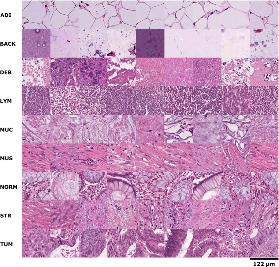
Figure 1: Sample images in PathMNIST

OCTMNIST [17]: This dataset composes of eye coherence tomography (OCT) images for diagnosing retinal diseases. It contains 109,309 samples (97477 for training, 10832 for validation, 1000 for testing) with four types of OCT images: Normal, CNV (Choroidal Neovascularization), DME (Diabetic Macular Edema) and Drusen (some kinds of desposits beneath retina). All the images from this dataset are naturally in grey scale.

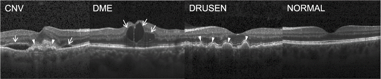
Figure 2: Sample images in OCTMNIST

PneumoniaMNIST [17]: A binary-classification dataset for diagnosing pneumonia through chest X-ray films. The original dataset includes 5856 cases (5232 for training and 624 for testing) and the training set was further split into training and validation with a 9:1 ratio.

OrganMNIST3D [3][33]: Comprising abdominal CT images, this dataset targets the classification of abdominal CT organs. This dataset contains 1,743 CT images (972 for training, 161 for validation, 610 for testing). 3D bounding boxes that contains the target organs are extracted from the raw CT images and resized to the same size for multi-class classification of 11 abdominal organs.

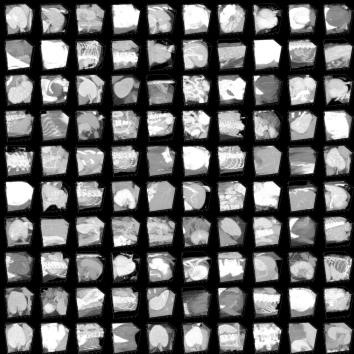
Figure 3: Sample images in OrganMNIST

VeseelMNIST3D [37]: This dataset is based on an open-access intracranial aneurysm dataset. This is a binary-class classification task for diagnosing the presence of aneurysm from cranial Magnetic Resonance Angiography. This dataset contains 1,694 normal artery segments and 215 aneurysm segments.

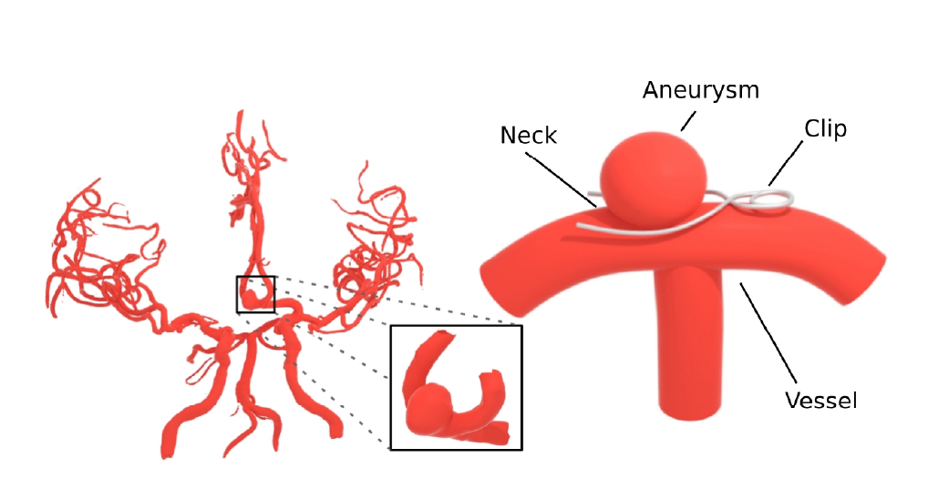
Figure 4: Sample images in VesselMNIST

The original datasets are treated as ground truth, assuming that they are all correctly labelled with no noise. To prove the robustness in learning with noisy labels, we simulated the real-world noisy data by corrupting some of the labels. We introduce artificial noise by randomly flipping the labels under noise rates from 0 (no noise) to 0.4. All the artificial label noise is added exclusively to the training set, so the validation and test set are still clean. We will evaluate the performance of different methods across varying noise rates: 0, 0.1, 0.2, 0.3, and 0.4.

4.2 Benchmark comparison methods

To efficacy the effectiveness of our proposed method, we implemented a benchmark baseline model and several state-of-the-art noise robust training methods for comparison. Where two of them (O2U-Net and Coteaching_plus) employed samples selection methods to filter data, and the sparse regularization method that we used was proposed by LNL_SR. Implementation details are in section 4.3.
Baseline: The baseline method is a common training procedure without using any noise-robust strategies. It serves as a simple benchmark only for comparative purposes.
O2U-Net [10]: This method uses three-phase training to remove the noisy data by ranking the loss values of all samples. More importantly, noticing the difficulty to judge whether the network is being overfitting or underfitting, the authors employed Cyclical Training to calculate the mean loss value through multiple epochs before filtering high-loss samples.
MixUp [39]: Mixup is a well-known data augmentation method, featuring simple but effective linear interpolation. This method is intended for avoiding overfitting in clean datasets, but has been proved useful on some noisy datasets as well.
Coteaching plus [38]: Coteaching-plus maintains two networks, each selecting small-loss samples to feed to the other network to learn from. Network parameters are updated based on samples where the networks disagree with each other.
CDR [32]: This is an early-stopping method designed to prevent the network from overfitting to noisy data. The authors categorize neural network parameters as important and none-important, employing early-stopping on the parameters that are more likely to cause overfitting.
Self-adaptive Training [11]: This is a label refurbishment method that corrects the labels by combining original labels with predictions and applying an exponential moving average strategy to stabilize the occasionally unreliable outputs of neural networks.
Multiclass [28]: This method employs a two-stage loss reweighting strategy to minimize the impact of incorrectly labeled cases. In the first stage, the model is pre-trained to calculate a weight transfusion matrix, which is then used in the second stage to estimate the true loss value of each sample.
LNL_SR [40]: LNL_SR adopts output permutation with sparse regularization to improve the robustness to noisy labels for any loss function, such as generalized cross entropy.

4.3 Implementation Details

We selected ResNet-18 as the backbone network for all experiments. The training batch size was set as 128 and training epochs were fixed as 200, aligning with the default settings in most comparison methods. The remaining hyperparameters of existing comparison methods are all retained in accordance with the original code. For the methods that need know the noise rate of the dataset to filter samples (O2U-Net and Coteaching_Plus), we set the noise rate to at constantly 0.2. These choices ensured the most fairness between different methods.

For the baseline (no noise-robustness) method, we choose Adam as the optimizer with an initial learning rate of 0.001. For our proposed method, the first and third phases were allocated 90 epochs each, with the remaining 20 epochs left for the second phase. Following LNL_SR, SGD optimizer with learning rate of 0.01 was applied in the first and third phases. While in the second phase, following the implementation details in O2U-Net, a smaller batch size of 16 was implemented and trained by a vanilla ResNet-18 and cross-entropy loss, with learning rate 0.01.

4.4 Evaluation metrics

All implemented methods in this study were assessed mainly using some metrics that are commonly employed in medical image classification tasks. Classification accuracy is our main metric, while precision (sensitivity), recall (specificity) and F1 score will also be used.

Furthermore, we construct receiver operating characteristic (ROC) curves for each method and calculate the corresponding area under the curve (AUC). T-SNE visualization was also employed to provide a more vivid presentation of the classification results, particularly in comparing the baseline method with our proposed methods.

4.5 Experiments on PathMNIST dataset

Noise rate	0.0	0.1	0.2	0.3	0.4
Baseline	97.79±1.45 88.96±2.06	94.62±0.50 86.01±0.58	88.61±2.02 78.85±1.22	80.09±1.20 70.08±0.25	71.94±1.54 63.60±1.87
O2U-Net	97.85±0.08 91.21±0.46	97.67±0.14 90.75±0.74	97.62±0.09 89.38±0.94	94.16±0.14 87.31±0.27	87.81±0.41 80.88±0.84
MixUp	99.37±0.10 87.61±0.83	96.73±0.45 85.95±1.05	92.72±0.81 83.60±1.67	86.31±1.42 77.68±1.91	76.34±1.04 68.59±1.14
Coteaching+	98.78±0.09 89.35±1.48	98.30±0.19 90.49±0.32	97.75±0.08 89.00±0.34	96.92±0.27 84.70±1.02	95.30±0.60 84.42±0.69
CDR	99.18±0.17 90.79±0.32	97.32±0.26 87.64±1.03	92.99±1.30 84.02±0.30	86.03±1.71 77.10±2.70	75.28±1.59 67.59±1.60
Self-adaptive	99.28±0.08 90.06±1.79	97.38±0.21 87.89±0.77	94.33±0.33 84.05±0.57	87.93±0.17 78.71±0.76	77.11±0.33 68.93±1.25
Multiclass	98.81±0.14 89.47±1.30	95.08±0.42 85.39±1.02	89.36±0.07 80.86±0.56	80.31±0.75 71.62±0.98	67.73±0.70 61.61±0.49
LNLSR	98.68±0.08 88.15±1.47	98.65±0.11 87.87±1.51	98.30±0.06 86.03±1.06	97.83±0.20 87.07±0.71	96.83±0.13 86.26±1.11
Ours	98.89±0.07 89.98±1.45	98.78±0.08 87.5±0.98	98.48±0.07 88.20±1.86	98.21±0.12 88.73±0.98	98.08±0.21 87.76±0.47

Table 1: Average accuracy (%, 3runs, with standard deviation) of different methods on PathMNIST validation / test dataset

	Baseline		Ours
	Validation set	Test set	Validation set	Test set
Precision	87.82	79.97	98.42	89.51
Recall	86.46	78.82	98.42	88.05
F1	86.60	79.01	98.42	87.98

Table 2: Precision, Recall and F1 score (%, Median of three runs) under noise rate 0.2.

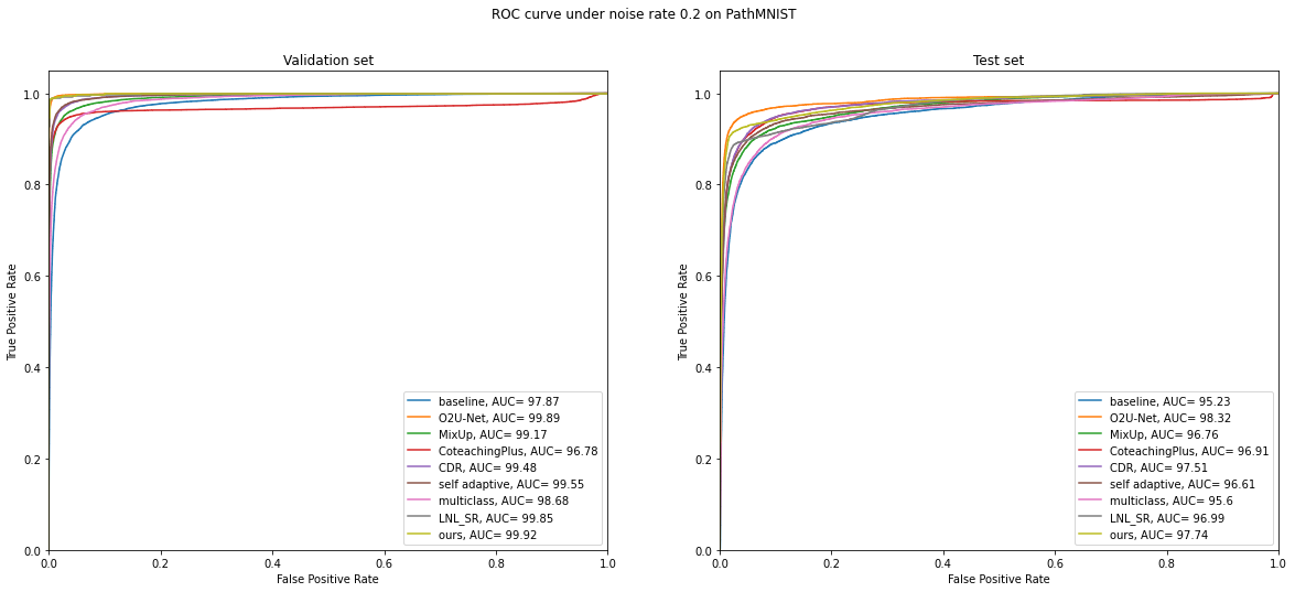
Figure 5: ROC curve and AUC of different methods on PathMNIST validation / test dataset under noise rate 0.2

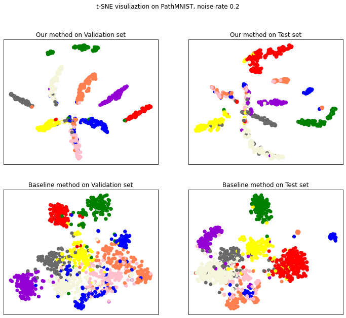
Figure 6: TSNE visualization of different methods on PathMNIST validation / test dataset under noise rate 0.2

Table 1 shows the classification accuracy of different noise-robust deep learning methods on PathMNIST validation and test datasets. Notably, it is clear that presence of label noise does degenerate the classification accuracy of all tested methods. As the noise ratio increases, the accuracy of all methods exhibits varying degrees of decline. Generally, the gap is still not big when noise rate changes from 0 to 0.2. However, a sharper decline in classification accuracy can be observed when noise rate further increases. Among them, the baseline method achieved the poorest overall accuracy.
Moreover, most of the existing noise-robust methods can more or less improve the accuracy score, depending on the noise rate settings. For instance, MixUp ranks first on the validation set when noise rate is 0, but fails to maintain this position in other conditions. Conversely, our original method win the first place across most of the noise rate settings, particularly when noise rate is very big and comparison methods show significant declines in accuracy score. Nevertheless, when the noise rate is small, our method is still competitive and obtains sub-optimal performance.
The ROC curves (figure 5) also illustrate the performance of our method under a mild noise rate of 0.2. The area under curve is consistent with the accuracy score and again confirmed the advantage of our method.
The precision, recall and F1 score metrics are available in Table 2. These figures and tables compare the performance of our method with the baseline method on PathMNIST dataset when noise rate is 0.2. It is observable that our method consistently demonstrates an obvious advantage over the baseline method various evaluation metrics.
Figure 6 shows the t-SNE visualization plot for our method and the baseline method under noise rate is 0.2. The visualization results manifest that the feature space of our method achieves better clustering effect than the baseline method.

Noise rate	0.0	0.1	0.2	0.3	0.4
Baseline	93.65±0.10 73.80±0.95	89.49±0.36 71.83±1.46	83.96±0.12 65.00±0.95	74.70±1.16 60.13±1.37	64.89±1.31 52.03±1.12
O2U-Net	91.41±0.13 74.13±1.40	92.18±0.07 73.23±0.57	92.42±0.14 73.43±1.67	88.05±0.64 67.47±0.35	80.61±1.09 59.10±1.30
MixUp	94.31±0.13 72.33±0.38	89.69±0.02 66.63±0.61	83.41±0.33 61.23±2.25	75.72±0.43 54.8±2.09	64.17±0.13 47.13±1.89
Coteaching+	93.37±0.19 75.97±0.67	92.67±0.50 74.23±2.08	89.66±0.70 69.20±0.66	85.28±0.35 66.33±1.29	82.78±1.71 62.10±2.71
CDR	94.31±0.13 75.50±1.13	90.20±0.28 70.57±2.23	84.81±0.37 65.00±0.95	77.45±0.22 59.93±1.60	65.81±0.18 47.30±1.73
Self-adaptive	94.30±0.10 74.37±0.40	90.44±0.14 71.60±0.66	84.74±0.60 66.23±0.23	76.59±0.68 61.37±0.40	65.65±0.68 51.37±1.44
Multiclass	94.22±0.17 75.47±1.19	89.47±0.14 70.30±0.66	83.13±1.59 64.50±0.66	76.39±1.27 60.80±0.87	61.43±4.61 45.03±2.81
LNLSR	93.73±0.04 76.33±0.06	93.05±0.18 74.27±0.59	92.18±0.13 73.56±2.02	90.34±0.57 72.53±0.38	90.37±0.05 71.70±1.04
Ours	93.89±0.20 76.50±0.26	93.29±0.19 74.97±0.12	92.35±0.23 74.67±0.50	91.35±0.14 73.07±1.24	90.34±0.19 72.30±1.04

Table 3: Average accuracy (%, 3runs, with standard deviation) of different methods on OCTMNIST validation / test dataset

	Baseline		Ours
	Validation set	Test set	Validation set	Test set
Precision	88.84	72.47	91.82	80.75
Recall	89.04	69.10	92.17	74.60
F1	88.87	65.76	91.90	72.16

Table 4: Precision, Recall and F1 score (%, Median of three runs) under noise rate 0.2.

Unlike the outcomes in PathMNIST dataset, the classification results in table 3 suggest that noisy OCTMNIST dataset is a much more difficult task for noise-robust learning methods. It can be observed from this table that compared with the non-robust baseline method, many existing noise-robust methods cannot really improve the performance on noisy OCTMNIST dataset, especially on the test set. For example, five out of the eight existing methods fail to outperform the baseline method when the noise rate is 0.2. However, even for this difficult task, our method still obtained top performance, closely followed by LNL_SR. This result proves the potential of our method in addressing the difficulties from more challenging noisy datasets.

Noise rate	0.0	0.1	0.2	0.3	0.4
Baseline	96.82±0.11 85.95±1.80	92.43±0.73 81.04±0.81	85.11±3.12 75.27±1.29	73.34±0.58 69.12±1.21	61.32±0.77 57.48±1.48
O2U-Net	96.88±0.40 85.42±0.80	94.46±0.83 82.69±0.70	88.61±3.29 79.54±1.62	78.69±4.30 74.20±2.20	62.72±0.30 60.47±2.65
MixUp	97.33±0.19 86.65±0.33	93.26±2.15 84.35±1.30	87.47±0.59 81.09±0.70	76.15±4.13 73.18±2.51	65.71±3.16 61.91±4.69
Coteaching+	95.67±0.48 85.10±1.95	96.44±0.40 81.36±0.82	92.62±1.72 81.36±2.60	86.32±5.61 76.65±1.64	76.78±13.8 71.10±10.7
CDR	96.75±0.33 85.15±0.09	93.89±0.33 82.00±0.18	86.33±1.98 77.25±3.16	77.35±4.19 68.53±1.29	62.72±0.44 60.31±2.59
Self-adaptive	96.37±0.33 85.79±0.96	90.97±0.44 79.76±1.57	80.66±0.77 73.77±2.98	73.47±1.63 65.92±0.24	60.94±0.94 57.75±2.40
Multiclass	96.69±0.12 84.29±0.43	96.64±0.11 81.20±1.22	86.70±1.76 76.92±1.21	76.84±2.92 71.10±1.69	66.16±2.98 60.58±3.24
LNLSR	96.44±0.58 85.37±0.18	96.31±0.40 84.24±0.25	95.17±0.44 85.1±0.55	92.43±0.29 81.03±2.98	73.73±1.73 65.22±1.16
Ours	96.56±0.58 84.83±0.61	96.63±0.12 85.04±0.89	96.18±0.11 85.15±1.49	96.15±0.44 83.65±2.12	89.31±3.03 75.53±0.56

Table 5: Average accuracy (%, 3runs, with standard deviation) of different methods on PneumoniaMNIST validation / test dataset

	Baseline		Ours
	Validation set	Test set	Validation set	Test set
Precision	85.29	76.78	96.37	87.46
Recall	84.35	76.44	96.37	86.22
F1	84.68	75.09	96.37	85.60

Table 6: Precision, Recall and F1 score (%, Median of three runs) under noise rate 0.2.

PneumoniaMNIST is another challenging task because this imbalanced binary classification dataset contains much more negative samples (no pneumonia) than positive samples (pneumonia). The experimental results are reported in table 5. For this binary-classification task, with noise rate increasing, the performance of most comparison methods will sharply decrease. For example, when noise rate rises from 0.3 to 0.4, a rapid decline in accuracy score can be observed in all existing methods, such as LNL_SR (18.7% in validation accuracy).
Conversely, our original method maintained excellent accurate score even when noise rate is very big. It is noticeable that when label noise existed (noise rate from 0.1 to 0.4), our method ranked first in all the experiments. Meanwhile, when the dataset was clean, MixUp obtained the highest accuracy score, indicating the efficacy of sample augmentation on clean datasets. Further validation of the performance of our method is presented in Table 6, evidently supporting our method’s superiority compared with the baseline. For this noisy binary classification task, samples are more clearly clustered by our method than the baseline, even with severely imbalanced data distribution.

4.6 Experiments on 3D benchmark datasets

In this part, we present the experimental results on two three-dimensional medical image datasets, including a CT dataset (OrganMNIST3D) and MRI dataset (VesselMNIST3D).

Noise rate	0.0	0.1	0.2	0.3	0.4
Baseline	97.93±0.95 90.49±0.43	97.52±0.63 83.99±0.81	94.80±0.95 79.40±1.92	84.06±0.72 68.96±1.58	75.57±1.80 59.45±3.09
O2U-Net	97.51±1.25 82.19±0.90	98.35±0.36 84.75±0.72	96.89±0.63 85.30±1.15	91.30±2.85 74.21±2.50	89.85±1.56 66.83±2.30
MixUp	98.35±0.95 92.51±1.51	96.55±0.79 84.44±0.68	90.13±3.55 77.83±1.42	81.16±3.99 68.58±3.78	75.57±2.59 62.19±2.61
Coteaching+	94.21±6.28 86.50±5.11	95.65±1.64 85.96±0.78	94.82±4.14 84.59±2.32	94.00±2.58 77.38±2.01	85.30±3.19 66.01±2.46
CDR	97.31±0.72 91.48±0.85	96.48±0.72 81.64±1.70	90.47±0.36 74.97±2.08	84.06±1.90 68.09±1.23	79.09±0.36 58.20±2.27
Self-adaptive	97.31±1.44 87.92±1.47	92.75±1.30 79.84±0.16	82.19±3.42 69.45±0.53	79.91±0.36 64.21±1.07	62.73±2.24 54.10±1.99
Multiclass	97.72±0.95 89.89±1.62	94.62±0.95 83.28±1.28	92.13±1.44 76.83±1.81	89.44±6.30 71.42±4.76	75.15±1.65 58.90±0.81
LNLSR	98.55±0.36 89.56±0.38	97.31±1.44 86.34±1.39	97.72±0.95 82.68±1.81	93.38±1.29 79.13±4.07	83.44±4.98 68.98±2.59
Ours	98.35±0.36 89.40±1.27	99.17±0.36 87.16±0.41	97.93±0.36 85.79±0.09	97.52±1.24 81.37±1.48	93.17±0.62 76.06±1.66

Table 7: Average accuracy (%, 3runs, with standard deviation) of different methods on OrganMNIST3D validation / test dataset

	Baseline		Ours
	Validation set	Test set	Validation set	Test set
Precision	95.92	86.57	98.58	86.57
Recall	95.65	85.74	98.13	85.74
F1	95.58	85.85	98.13	85.87

Table 8: Precision, Recall and F1 score (%, Median of three runs) under noise rate 0.2.

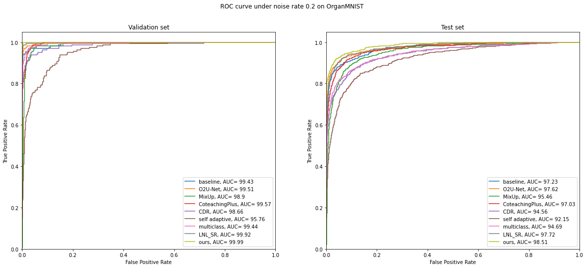
Figure 7: ROC curve and AUC of different methods on OrganMNIST3D validation / test dataset under noise rate 0.2

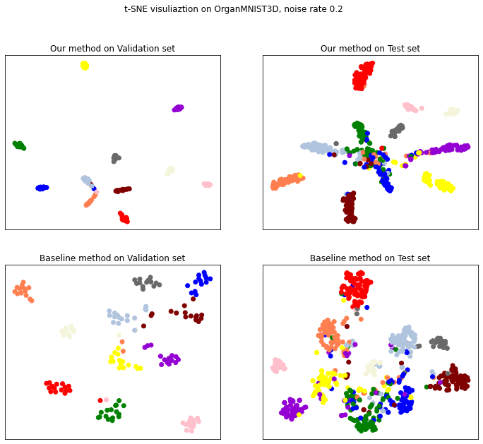
Figure 8: TSNE visualization of different methods on OrganMNIST3D validation / test dataset under noise rate 0.2

Table 7 presents the outcomes of our method and other competitors on OrganMNIST3D dataset. In this challenging 3D abdominal CT classification task, our method obtained sub-optimal results on a clean dataset, and as noise rate increases, the advantage of our method is even more apparent, outperforming its competitors across all noise rate settings. This advantage can also be illustrated by ROC curve (Figure 7) under noise rate 0.2. The t-SNE visualization in Figure 8 also proves that our method is not impacted by the 3D nature of abdominal CT images.
This study marks the first exploration of whether current noise-robust deep learning methods still work on 3D medical images. The results in this experiment reveal that the efficacy of noise-robust learning methods is not solely determined by the dimensionality of medical images. Most of the existing noise-robust learning methods designed for 2D images still exhibit varying degrees of efficacy on 3D medical images. Among them, our original method again obtains the highest level of robustness, particularly in handling extremely noisy data.

Noise rate	0.0	0.1	0.2	0.3	0.4
Baseline	91.49±1.97 90.84±1.36	87.85±1.97 87.00±2.03	82.47±2.11 82.11±1.49	70.48±1.50 68.76±1.68	63.37±4.37 62.83±4.65
O2U-Net	90.28±1.09 90.75±1.53	90.27±0.60 90.49±1.06	79.86±4.67 79.23±1.09	67.02±0.79 70.33±3.57	64.24±2.11 58.55±1.75
MixUp	92.54±0.79 92.15±1.36	84.72±3.39 84.91±1.58	76.04±7.68 77.49±5.50	68.23±0.52 68.06±1.89	59.38±7.35 59.42±4.21
Coteaching+	89.58±1.04 88.48±0.26	91.49±1.51 91.01±1.34	86.29±0.60 85.69±3.54	76.21±4.24 76.97±2.24	63.72±2.11 64.83±2.11
CDR	93.58±1.20 92.32±0.15	87.67±0.30 87.26±0.76	84.55±3.31 80.28±2.88	76.39±3.00 71.29±1.66	56.95±5.71 62.22±1.66
Self-adaptive	91.49±0.80 91.62±1.20	86.28±2.17 83.94±1.06	75.17±5.22 79.15±2.42	75.52±10.8 73.04±11.6	59.03±4.92 56.89±3.93
Multiclass	94.44±0.30 92.67±1.05	92.02±0.30 89.79±0.26	83.16±4.21 81.85±2.63	73.96±3.13 72.34±3.71	68.75±10.1 64.40±1.63
LNLSR	90.10±1.05 91.27±0.54	89.06±1.87 89.88±0.40	87.85±1.31 87.00±1.06	81.02±7.29 83.34±5.26	70.83±5.63 73.12±1.29
Ours	90.27±0.30 89.70±0.65	89.93±0.30 90.23±0.84	89.06±2.27 88.48±1.45	85.07±1.20 85.95±1.44	83.86±0.91 83.24±2.77

Table 9: Average accuracy (%, 3runs, with standard deviation) of different methods on VesselMNIST3D validation / test dataset

	Baseline		Ours
	Validation set	Test set	Validation set	Test set
Precision	87.43	84.48	82.37	85.69
Recall	82.81	80.89	85.94	88.74
F1	84.60	82.46	83.81	86.11

Table 10: Precision, Recall and F1 score (%, Median of three runs) under noise rate 0.2.

VesselMNIST is another imbalance 3D dataset, which is also a challenge for all methods. We can see that our method successfully obtained the higher score on this difficult dataset.

From table 9, it can be observed that in VesselMNSIT dataset, our method still ranked top in all the experiments. Especially, when the noise rate is big, our method surpassed the second-best method by more than 10% in classification accuracy. This robust performance demonstrates our method’s ability of finding a good way to learn the correct knowledge from heavily noisy samples. Furthermore, even in situations with small label noise, our method still obtained an acceptable classification performance.

In summary, an examination of the two datasets reveals that the dimensionality of the dataset is not the sole determinant of the efficacy of noise-robust deep learning models. Most of the existing methods exhibit a comparable performance on both 3D and 2D datasets. Among them, our proposed method demonstrates a high level of superiority compared with other existing methods, underscoring its high performance on 3D medical images. This study substantiates the potential effectiveness of noise-robust learning in the context of 3D medical images, which makes up a big proportion of contemporary medical applications.

4.7 Performance of noise rate estimation module and ablation study

In this section, we conducted a comparison between the predicted noise rate generated by our module and the actual noise rate, aiming to assess the prediction ability of this module. The detailed results are presented in table 11, showing that for most datasets, our predictions closely align with the actual noise rate.
Notably, for the OrganMNIST with noise rate 0, our model exhibit a mean prediction of 0.165, which is quite different from the actual noise rate 0. Despite this anomaly, the difference is still in an accepted range. These findings prove the effectiveness of our noise rate estimation module. Although based on a straightforward linear regression model, this module expresses high efficacy in predicting the noise level of a given medical image dataset.

Actual noise rate	0	0.1	0.2	0.3	0.4
Path	0.005	0.079	0.173	0.267	0.362
OCT	0	0.133	0.226	0.340	0.449
Pneumonia	0	0.068	0.162	0.257	0.382
Organ	0.165	0.176	0.256	0.316	0.364
Vessel	0.072	0.142	0.236	0.265	0.392

Table 11: Average predicted noise rate over three runs.

To better understand the role of the noise rate estimation module and its influence of the classification results, an ablation study with different forget rates is performed across the five datasets. We set five different fixed forget rates (0 to 0.4) and compared the classification accuracy of our original noise-robust learning method of the fixed and estimated forget rates.
The findings detailed in table 12 indicate an improvement in overall classification accuracy dues to our adaptive noise rate estimation module when compared to a fixed noise rate. Notably, with the integration of this noise rate estimation module, the overall accuracy outperforms that of small forget rates (0 and 0.1) on all datasets, and outperforms big forget rates (0.2, 0.3, 0.4) on most datasets. These results signify the potential of this noise-rate estimation module to enhance practical applicability of our sample selection method, showing potential in clinical datasets where the noise rate of a dataset is unknown.

Forget rate	0.0	0.1	0.2	0.3	0.4	Estimated
PathMNIST	98.39 88.22	98.34 88.12	98.00 88.06	97.68 89.20	97.40 89.27	98.43 88.58
OCTMNIST	91.59 72.74	91.54 72.02	91.61 73.44	91.76 72.96	92.13 73.56	92.24 74.30
PneumoniaMNIST	89.96 79.01	91.53 80.32	93.89 81.54	94.54 80.42	90.57 77.76	94.63 82.97
OrganMNIST3D	96.03 81.61	95.41 82.26	98.14 81.48	97.02 83.90	96.28 83.15	97.23 83.96
VesselMNIST3D	84.69 85.34	82.29 82.67	87.08 87.22	88.44 88.74	86.77 86.75	87.64 87.52

Table 12: The overall average accuracy score (%) under different noise rates of various forget rate settings.

5 Conclusion

In this paper, we present a noise-robust deep learning method designed for the classification of diverse medical images with label noise. This method consists of three modules tailored for noise robustness: noise rate estimation, sample selection, and sparse regularization. Experiments with both 2D and 3D medical image datasets were conducted to evaluate the proposed method. The outcomes demonstrate the efficacy of this method in enhancing classification performance across varying levels of label noise, particularly in severely noisy datasets. Future work will apply this proposed model to real-life medical image datasets.

References

- [1] Devansh Arpit, Stanisaw Jastrzbski, Nicolas Ballas, David Krueger, Emmanuel Bengio, Maxinder S Kanwal, Tegan Maharaj, Asja Fischer, Aaron Courville, Yoshua Bengio, et al. A closer look at memorization in deep networks. In International conference on machine learning, pages 233–242. PMLR, 2017.
- [2] David Berthelot, Nicholas Carlini, Ian Goodfellow, Nicolas Papernot, Avital Oliver, and Colin A Raffel. Mixmatch: A holistic approach to semi-supervised learning. Advances in neural information processing systems, 32, 2019.
- [3] Patrick Bilic, Patrick Christ, Hongwei Bran Li, Eugene Vorontsov, Avi Ben-Cohen, Georgios Kaissis, Adi Szeskin, Colin Jacobs, Gabriel Efrain Humpire Mamani, Gabriel Chartrand, et al. The liver tumor segmentation benchmark (lits). Medical Image Analysis, 84:102680, 2023.
- [4] Pete Bridge, Andrew Fielding, Pamela Rowntree, and Andrew Pullar. Intraobserver variability: should we worry?, 2016.
- [5] S Sreenivasa Chakravarthi, S Sountharrajan, B Narendra Kumar Rao, E Suganya, M Nivaashini, et al. Sparsely supervised learning for medical image classification on noisy heterogeneous data. In 2023 3rd International Conference on Advance Computing and Innovative Technologies in Engineering (ICACITE), pages 1617–1621. IEEE, 2023.
- [6] Pengfei Chen, Ben Ben Liao, Guangyong Chen, and Shengyu Zhang. Understanding and utilizing deep neural networks trained with noisy labels. In International Conference on Machine Learning, pages 1062–1070. PMLR, 2019.
- [7] Yair Dgani, Hayit Greenspan, and Jacob Goldberger. Training a neural network based on unreliable human annotation of medical images. In 2018 IEEE 15th International symposium on biomedical imaging (ISBI 2018), pages 39–42. IEEE, 2018.
- [8] Bo Han, Quanming Yao, Xingrui Yu, Gang Niu, Miao Xu, Weihua Hu, Ivor Tsang, and Masashi Sugiyama. Co-teaching: Robust training of deep neural networks with extremely noisy labels. Advances in neural information processing systems, 31, 2018.
- [9] Tingxin Hu, Bingyu Yang, Jia Guo, Weihang Zhang, Hanruo Liu, Ningli Wang, and Huiqi Li. A fundus image classification framework for learning with noisy labels. Computerized Medical Imaging and Graphics, 108:102278, 2023.
- [10] Jinchi Huang, Lie Qu, Rongfei Jia, and Binqiang Zhao. O2u-net: A simple noisy label detection approach for deep neural networks. In Proceedings of the IEEE/CVF international conference on computer vision, pages 3326–3334, 2019.
- [11] Lang Huang, Chao Zhang, and Hongyang Zhang. Self-adaptive training: beyond empirical risk minimization. Advances in neural information processing systems, 33:19365–19376, 2020.
- [12] Hongyang Jiang, Mengdi Gao, Yan Hu, Qiushi Ren, Zhaoheng Xie, and Jiang Liu. Label-noise-tolerant medical image classification via self-attention and self-supervised learning. arXiv preprint arXiv:2306.09718, 2023.
- [13] Lu Jiang, Zhengyuan Zhou, Thomas Leung, Li-Jia Li, and Li Fei-Fei. Mentornet: Learning data-driven curriculum for very deep neural networks on corrupted labels. In International conference on machine learning, pages 2304–2313. PMLR, 2018.
- [14] Davood Karimi, Haoran Dou, Simon K Warfield, and Ali Gholipour. Deep learning with noisy labels: Exploring techniques and remedies in medical image analysis. Medical image analysis, 65:101759, 2020.
- [15] Davood Karimi, Guy Nir, Ladan Fazli, Peter C Black, Larry Goldenberg, and Septimiu E Salcudean. Deep learning-based gleason grading of prostate cancer from histopathology images—role of multiscale decision aggregation and data augmentation. IEEE journal of biomedical and health informatics, 24(5):1413–1426, 2019.
- [16] Jakob Nikolas Kather, Johannes Krisam, Pornpimol Charoentong, Tom Luedde, Esther Herpel, Cleo-Aron Weis, Timo Gaiser, Alexander Marx, Nektarios A Valous, Dyke Ferber, et al. Predicting survival from colorectal cancer histology slides using deep learning: A retrospective multicenter study. PLoS medicine, 16(1):e1002730, 2019.
- [17] Daniel S Kermany, Michael Goldbaum, Wenjia Cai, Carolina CS Valentim, Huiying Liang, Sally L Baxter, Alex McKeown, Ge Yang, Xiaokang Wu, Fangbing Yan, et al. Identifying medical diagnoses and treatable diseases by image-based deep learning. cell, 172(5):1122–1131, 2018.
- [18] Bidur Khanal, Binod Bhattarai, Bishesh Khanal, and Cristian A Linte. Improving medical image classification in noisy labels using only self-supervised pretraining. In MICCAI Workshop on Data Engineering in Medical Imaging, pages 78–90. Springer, 2023.
- [19] Jonathan Krause, Benjamin Sapp, Andrew Howard, Howard Zhou, Alexander Toshev, Tom Duerig, James Philbin, and Li Fei-Fei. The unreasonable effectiveness of noisy data for fine-grained recognition. In Computer Vision–ECCV 2016: 14th European Conference, Amsterdam, The Netherlands, October 11-14, 2016, Proceedings, Part III 14, pages 301–320. Springer, 2016.
- [20] Junnan Li, Richard Socher, and Steven CH Hoi. Dividemix: Learning with noisy labels as semi-supervised learning. arXiv preprint arXiv:2002.07394, 2020.
- [21] Jiarun Liu, Ruirui Li, and Chuan Sun. Co-correcting: noise-tolerant medical image classification via mutual label correction. IEEE Transactions on Medical Imaging, 40(12):3580–3592, 2021.
- [22] Eran Malach and Shai Shalev-Shwartz. Decoupling” when to update” from” how to update”. Advances in neural information processing systems, 30, 2017.
- [23] Giorgio Patrini, Alessandro Rozza, Aditya Krishna Menon, Richard Nock, and Lizhen Qu. Making deep neural networks robust to label noise: A loss correction approach. In Proceedings of the IEEE conference on computer vision and pattern recognition, pages 1944–1952, 2017.
- [24] Hieu H Pham, Tung T Le, Dat Q Tran, Dat T Ngo, and Ha Q Nguyen. Interpreting chest x-rays via cnns that exploit hierarchical disease dependencies and uncertainty labels. Neurocomputing, 437:186–194, 2021.
- [25] Yanyao Shen and Sujay Sanghavi. Learning with bad training data via iterative trimmed loss minimization. In International Conference on Machine Learning, pages 5739–5748. PMLR, 2019.
- [26] Hwanjun Song, Minseok Kim, Dongmin Park, Yooju Shin, and Jae-Gil Lee. Robust learning by self-transition for handling noisy labels. In Proceedings of the 27th ACM SIGKDD Conference on Knowledge Discovery & Data Mining, pages 1490–1500, 2021.
- [27] Sainbayar Sukhbaatar, Joan Bruna, Manohar Paluri, Lubomir Bourdev, and Rob Fergus. Training convolutional networks with noisy labels. arXiv preprint arXiv:1406.2080, 2014.
- [28] Ruxin Wang, Tongliang Liu, and Dacheng Tao. Multiclass learning with partially corrupted labels. IEEE transactions on neural networks and learning systems, 29(6):2568–2580, 2017.
- [29] Yisen Wang, Xingjun Ma, Zaiyi Chen, Yuan Luo, Jinfeng Yi, and James Bailey. Symmetric cross entropy for robust learning with noisy labels. In Proceedings of the IEEE/CVF international conference on computer vision, pages 322–330, 2019.
- [30] Hongxin Wei, Lei Feng, Xiangyu Chen, and Bo An. Combating noisy labels by agreement: A joint training method with co-regularization. In Proceedings of the IEEE/CVF conference on computer vision and pattern recognition, pages 13726–13735, 2020.
- [31] Zhi-Fan Wu, Tong Wei, Jianwen Jiang, Chaojie Mao, Mingqian Tang, and Yu-Feng Li. Ngc: A unified framework for learning with open-world noisy data. In Proceedings of the IEEE/CVF International Conference on Computer Vision, pages 62–71, 2021.
- [32] Xiaobo Xia, Tongliang Liu, Bo Han, Chen Gong, Nannan Wang, Zongyuan Ge, and Yi Chang. Robust early-learning: Hindering the memorization of noisy labels. In International conference on learning representations, 2020.
- [33] Xuanang Xu, Fugen Zhou, Bo Liu, Dongshan Fu, and Xiangzhi Bai. Efficient multiple organ localization in ct image using 3d region proposal network. IEEE transactions on medical imaging, 38(8):1885–1898, 2019.
- [34] Cheng Xue, Qi Dou, Xueying Shi, Hao Chen, and Pheng-Ann Heng. Robust learning at noisy labeled medical images: Applied to skin lesion classification. In 2019 IEEE 16th International Symposium on Biomedical Imaging (ISBI 2019), pages 1280–1283. IEEE, 2019.
- [35] Cheng Xue, Lequan Yu, Pengfei Chen, Qi Dou, and Pheng-Ann Heng. Robust medical image classification from noisy labeled data with global and local representation guided co-training. IEEE Transactions on Medical Imaging, 41(6):1371–1382, 2022.
- [36] Jiancheng Yang, Rui Shi, Donglai Wei, Zequan Liu, Lin Zhao, Bilian Ke, Hanspeter Pfister, and Bingbing Ni. Medmnist v2-a large-scale lightweight benchmark for 2d and 3d biomedical image classification. Scientific Data, 10(1):41, 2023.
- [37] Xi Yang, Ding Xia, Taichi Kin, and Takeo Igarashi. Intra: 3d intracranial aneurysm dataset for deep learning. In Proceedings of the IEEE/CVF Conference on Computer Vision and Pattern Recognition, pages 2656–2666, 2020.
- [38] Xingrui Yu, Bo Han, Jiangchao Yao, Gang Niu, Ivor Tsang, and Masashi Sugiyama. How does disagreement help generalization against label corruption? In International Conference on Machine Learning, pages 7164–7173. PMLR, 2019.
- [39] Hongyi Zhang, Moustapha Cisse, Yann N Dauphin, and David Lopez-Paz. mixup: Beyond empirical risk minimization. arXiv preprint arXiv:1710.09412, 2017.
- [40] Xiong Zhou, Xianming Liu, Chenyang Wang, Deming Zhai, Junjun Jiang, and Xiangyang Ji. Learning with noisy labels via sparse regularization. In Proceedings of the IEEE/CVF international conference on computer vision, pages 72–81, 2021.
- [41] Chuang Zhu, Wenkai Chen, Ting Peng, Ying Wang, and Mulan Jin. Hard sample aware noise robust learning for histopathology image classification. IEEE transactions on medical imaging, 41(4):881–894, 2021.
- [42] Minjuan Zhu, Lei Zhang, Lituan Wang, Dong Li, Jianwei Zhang, and Zhang Yi. Robust co-teaching learning with consistency-based noisy label correction for medical image classification. International Journal of Computer Assisted Radiology and Surgery, 18(4):675–683, 2023.