PERP: Rethinking the Prune-Retrain Paradigm in the Era of LLMs

Abstract

Neural Networks can be efficiently compressed through pruning, significantly reducing storage and computational demands while maintaining predictive performance. Simple yet effective methods like Iterative Magnitude Pruning (IMP) (Han et al., 2015) remove less important parameters and require a costly retraining procedure to recover performance after pruning. However, with the rise of Large Language Models (LLMs), full retraining has become infeasible due to memory and compute constraints. In this study, we challenge the practice of retraining all parameters by demonstrating that updating only a small subset of highly expressive parameters is often sufficient to recover or even improve performance compared to full retraining. Surprisingly, retraining as little as 0.27%-0.35% of the parameters of GPT-architectures achieves comparable performance to One Shot IMP across various sparsity levels. Our approach, Parameter-Efficient Retraining after Pruning (PERP), drastically reduces compute and memory demands, enabling pruning and retraining of up to 30 billion parameter models on a single NVIDIA A100 GPU within minutes. Despite magnitude pruning being considered as unsuited for pruning LLMs, our findings show that PERP positions it as a strong contender against state-of-the-art retraining-free approaches such as Wanda (Sun et al., 2023) and SparseGPT (Frantar & Alistarh, 2023), opening up a promising alternative to avoiding retraining.

1 Introduction

Pruning (Han et al., 2015; Gale et al., 2019; Lin et al., 2020; Hoefler et al., 2021; Zimmer et al., 2022) is among the state-of-the-art techniques to reduce the compute and storage requirements of Neural Networks, allowing to benefit from the extensive over-parametrization of modern architectures (Zhang et al., 2016) throughout training while maintaining high performance with lower resource demands during deployment. Arguably simple yet effective approaches to obtaining such sparse models follow the prune after training paradigm and are exemplified by Iterative Magnitude Pruning (IMP) (Han et al., 2015), which starts from a pretrained dense model and iteratively removes seemingly unimportant parameters followed by retraining to compensate for pruning-induced performance degradation.

Despite its popularity, IMP suffers from being computationally expensive, potentially having to perform many prune-retrain cycles and retraining epochs to obtain well-performing models that are sufficiently compressed for the task at hand. Especially given the surge in popularity of transfer learning, in which huge pretrained models are reused and fine-tuned to specific tasks, a procedure such as IMP can be prohibitive for practitioners dealing with resource constrained environments (Frantar & Alistarh, 2023), even when performing just a single prune-retrain cycle (One Shot). In that vein, retraining itself enjoys a particularly negative reputation and a variety of pruning approaches try to avoid it entirely. These include novel weight-selection criteria for pruning without the need for retraining (Frantar & Alistarh, 2023; Sun et al., 2023), and prune during training strategies (Liu et al., 2020; Ding et al., 2019; Lin et al., 2020; Wortsman et al., 2019), which aim to achieve sparsity at the end of the regular training process.

Several works have tried to address the issue from the angle of making retraining itself less undesirable. Zimmer et al. (2023) accelerate retraining using a pruning-adaptive learning rate schedule, effectively reducing the number of iterations required while improving generalization performance. To find lottery tickets (Frankle & Carbin, 2018) more efficiently, You et al. (2020) and Wolfe et al. (2021) try to find the pruning mask earlier in training, Jaiswal et al. (2023b) speed up the mask-generation process by superimposing a set of masks throughout retraining, and Zhang et al. (2021) reduce the number of retraining iterations by using only a critical subset of the data. Zimmer et al. (2024) show that constructing sparse model soups during each phase of IMP can enhance its performance and consequently reduce the overall wall-time required for retraining.

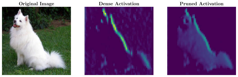
Figure 1: Features produced by a single filter from the first convolutional layer of AlexNet (Krizhevsky et al., 2012). From left to right: original image, output from a pretrained model, and output from the magnitude-pruned version of the same model.

In this work, we propose viewing the problem from yet another, previously unexplored angle, namely that of parameter-efficiency. To the best of our knowledge, all classical methods define retraining after pruning as a retraining of all parameters at hand, requiring computation and storage of full gradients at each step. This is particularly challenging with optimizers like Adam (Kingma & Ba, 2014), which need storage for parameters, gradients, and both first and second-order moments. As a result, retraining all parameters emerges as a challenge both in terms of computational efficiency and storage demands, especially in the context of Large Language Models (LLMs) (Frantar & Alistarh, 2023; Sun et al., 2023). Yet, retraining often requires much fewer iterations than training from scratch (Zimmer et al., 2023), suggesting that pruned models retain considerable feature information despite diminished performance.

Inspired by the recent advancements in Parameter-Efficient Fine-Tuning (PEFT) (Lialin et al., 2023a) that enable large-scale model fine-tuning on standard hardware (Lialin et al., 2023b), we challenge the common practice of retraining all parameters after pruning. We view pruning as a process of feature distortion and emphasize the similarity between the transfer learning setting and the prune-retrain paradigm. Our findings indicate that retrained models can remain closely aligned with their pruned versions, suggesting significant feature preservation, despite initial pruning-induced performance drops to near-random levels. Surprisingly, by retraining as little as 0.27%-0.35% of the parameters of the Generative Pretrained Transformer (GPT) architectures OPT-2.7B/6.7B/13B/30B/66B (Zhang et al., 2022), LLaMA-2-7B/13B/70B (Touvron et al., 2023), Mistral-7B (Jiang et al., 2023) as well as Mixtral-8x7B (Mistral, 2023), we achieve nearly all of IMP’s performance in the One Shot setting with moderate to high sparsity levels, where magnitude pruning without retraining collapses entirely. By drastically reducing the memory requirements for retraining, we are able to prune and retrain up to 30 billion parameter GPT s on a single NVIDIA A100 GPU. Similarly, retraining 0.004%-0.21% of the parameters of a ResNet-50 on ImageNet is for many sparsity levels sufficient to recover the accuracy after pruning. Our investigation of state-of-the-art PEFT approaches for retraining after pruning opens a promising alternative to avoiding retraining entirely, which we refer to as Parameter-Efficient Retraining after Pruning (PERP).

To sum up, our main contributions are:

1. Restoring feature quality with few parameters. We challenge the practice of retraining all parameters after pruning, demonstrating that retraining a small subset of highly expressive parameters can effectively restore performance after One Shot pruning, with backpropagation of less than 1% of the total parameters often sufficing for full recovery. Motivated by the investigation of state-of-the-art Parameter-Efficient Fine-Tuning (PEFT) in the prune-retrain context, we propose Parameter-Efficient Retraining after Pruning (PERP), using a fraction of the parameters and retraining with drastically reduced compute and memory requirements. We extend our findings to the setting of multiple prune-retrain cycles, where we match IMP’s performance with less aggregated memory and compute demands.

2. Making retraining of large models feasible. We validate our approach through comprehensive experiments across Natural Language Processing (NLP) and Image Classification. Notably, we backpropagate as little as 0.27%-0.35% of parameters of OPT-GPT s, LLaMA-2 and Mistral models, utilizing a single NVIDIA A100 to retrain up to 30 billion parameter models within minutes. Further, we recover most of the accuracy of full retraining by utilizing 0.004%-0.21% of ResNet-50 parameters on ImageNet across various sparsity levels.

3. Reconsidering Magnitude Pruning of LLMs. Despite being recognized as unsuited for LLMs due to exploding perplexity at moderate sparsity levels, we demonstrate that PERP reduces the perplexity of magnitude pruning by several orders of magnitude with minimal iterations on less than 1% of the parameters, and further also improves state-of-the-art retraining-free methods like SparseGPT (Frantar & Alistarh, 2023) and Wanda (Sun et al., 2023). Our results reveal that magnitude pruning coupled with PERP remains a viable and competitive option in the unstructured as well as semi-structured 2:4 and 4:8 sparsity settings.

2 Methodology and Experimental Setup

2.1 Preliminaries

We begin with a quick overview of pruning and transfer learning, which are central to our study.

Pruning. We prune Neural Networks in a post-hoc fashion, removing individual weights as is done by the previously introduced IMP approach. IMP adopts the prune after training paradigm, consisting of three-stages: i) pretraining to convergence, ii) permanently pruning the smallest magnitude weights, and iii) retraining to recover the predictive performance eradicated by pruning. These last two stages, often termed a prune-retrain cycle or phase, are either performed once (One Shot) or repeated until a desired level sparsity is met. Despite its straightforward nature, IMP and its variants have been shown to produce sparse models comparable in performance to those from more complex algorithms (Gale et al., 2019; Zimmer et al., 2023). In this work, we focus on IMP’s potential to produce high-quality sparse models rather than lottery tickets.

Pruning a non-trivial portion of the parameters typically results in significant performance degradation. In consequence, the retraining step is fundamental in each phase, mainly for two reasons: First of all, it enables recovery from pruning-induced performance drops, typically in much fewer iterations than what standard training would require to achieve a comparable reduction in train loss (Zimmer et al., 2023). Furthermore, it prepares the network for subsequent prune-retrain cycles, mitigating layer-collapse; a phenomenon where excessive pruning in a single phase entirely eliminates a layer, rendering the model dysfunctional (Tanaka et al., 2020). Without retraining between pruning steps, the final IMP result would be equal to One Shot IMP.

While the magnitude criterion is widely used, it is by far not the only one, as detailed in studies like LeCun et al. (1989); Hassibi & Stork (1993); Molchanov et al. (2016); Yeom et al. (2019). For a comprehensive review, we refer to Hoefler et al. (2021). This study primarily focuses on magnitude pruning, but in Section 3.3, we also discuss recent pruning strategies designed for LLMs to avoid retraining entirely.

Transfer learning. As models grow in size, Fine-Tuning (FT) —the process of adapting a pretrained or foundation model to a novel task—has become the norm, avoiding the inefficiencies of training from scratch for each new task (Houlsby et al., 2019; Kumar et al., 2022b). FT capitalizes on the transfer of existing knowledge to a closely related domain (transfer learning). Yet, the immense size and complexity of foundation models can make the traditional FT approach more challenging, requiring storage for the entire model, its gradients, and auxiliary buffers, even for brief training. In response, various Parameter-Efficient Fine-Tuning (PEFT) methods have emerged. They significantly reduce the number of trainable parameters, cutting down on compute and storage needs, while preserving performance levels comparable to conventional FT.

PEFT methods are broadly categorized as selective, additive, or reparametrization-based (Lialin et al., 2023a). Selective methods update specific model components, such as the top linear layer (Kumar et al., 2022a; Evci et al., 2022), only the biases (Zaken et al., 2021), or by partitioning specific tensors into active and inactive portions (Vucetic et al., 2022). Additive methods, like adapters (Houlsby et al., 2019; He et al., 2022), add new parameters which are trained for specific tasks while the main model remains unchanged. Reparametrization-based methods exploit the low intrinsic dimensionality of fine-tuning (Aghajanyan et al., 2020). A well-known example is Low-Rank Adaptation (LoRA) (Hu et al., 2021), which implicitly enforces low-rank constraints on additive updates to pretrained parameter matrices, substantially decreasing the number of trainable parameters.

Precisely, LoRA freezes the pretrained parameters and reparametrizes each weight matrix $W_{0}\in\mathbb{R}^{n\times m}$ as $W_{0}+\Delta W$, where $\Delta W=BA$ represents the update matrix. In this representation, $B\in\mathbb{R}^{n\times r}$ and $A\in\mathbb{R}^{r\times m}$ implicitly constrain the rank of $\Delta W$ to be at most $r\ll\min(n,m)$. $B$ is initialized with zeros, allowing the reparametrization to preserve the original model’s behavior. During training, only $A$ and $B$ are updated, while $W_{0}$ remains fixed.

Other related literature. Kwon et al. (2022) propose a structured pruning framework for transformers, explicitly avoiding retraining for efficiency. Zhang et al. (2023b) develop a training-free pruning method inspired by prune-and-grow strategies from Dynamic Sparse Training (Evci et al., 2020). Ding et al. (2019) and Liu et al. (2020) propose pruning methods that circumvent the perceived high costs of retraining. Several works propose techniques in the domain of sparse fine-tuning in transfer learning. Zhang et al. (2023a) address the problem of performing gradient-based pruning by utilizing the LoRA gradients. Liu et al. (2021) aim at pruning pretrained models for improvements when fine-tuning to downstream tasks. Li et al. (2022) reduce the number of parameters for weight importance computation in sparse fine-tuning. While conventional retraining typically involves retraining all parameters, some may have implicitly employed PEFT in pruning LLMs, e.g., Sun et al. (2023) further fine-tune their sparse model using LoRA. To the best of our knowledge, our work is the first to extensively explore PEFT in the context of retraining after pruning.

2.2 Parameter-Efficient Retraining After Pruning

Pruning can degrade the model’s performance to near-random levels. Yet, retraining often restores performance in much fewer iterations than similar loss reductions during pretraining (Zimmer et al., 2023). This optimization often involves merely a few iterations, even when dealing with substantial pruning-induced performance degradation. Consequently, even if the pruned network is severely damaged, it likely retains most of the task-informative features. We hypothesize that, similar to fine-tuning in transfer learning, retraining can be significantly more efficient by leveraging these features rather than adjusting the entire network, despite pruning severely damaging the model.

More specifically, we observe that the transfer learning paradigm—shifting from source to target domain and subsequent fine-tuning—bears a resemblance to the prune-retrain paradigm. In transfer learning, the optimization objective changes with a new task, requiring fine-tuning. Pruning, which permanently sets parameters to zero, limits the optimization to a linear subspace and increases the model’s error, despite identical source and target space. However, an alternative view on pruning is as a disturbance to the features the model has learned. This disruption means the model needs to be retrained to align with the original domain’s features. In essence, retraining after pruning is about refining imperfect, yet valuable features.

Figure 1 illustrates this intuition by depicting a dog (left) and the features produced by a single filter from the first convolutional layer of a pretrained network (middle) and its pruned version (right). The middle image demonstrates the pretrained network’s capability to capture distinct boundary features, especially the dog’s defining back and ears. Conversely, the pruned network still emphasizes the dog’s back, albeit with reduced intensity and in favor of its overall form, likely influenced by the stark contrast between the white dog and the green grass. While pruning diminishes the feature quality, it does not completely eradicate it.

What gains can we expect from parameter-efficiency? Parameter-Efficient Retraining aims to substantially reduce the computational load and memory demands of backpropagation by retraining fewer parameters, i.e., freezing the majority of parameters to not require gradients. While computational speedups are not always guaranteed, as techniques like adapters or LoRA might increase computational requirements, we especially expect selective methods to boost performance. However, a major benefit also lies in the significant reduction in memory requirements. This reduction is crucial for retraining large models efficiently, exemplified by our ability to retrain the 30 billion parameter model OPT-30B on a single NVIDIA A100-80GB within minutes. Typically, optimizers such as AdamW (Kingma & Ba, 2014; Loshchilov & Hutter, 2019) require multiple buffers for each parameter, including the parameter itself, its gradient, and both first and second-order moments. Involving fewer parameters results in considerably less allocated memory. Additionally, the memory required for storing activations during backpropagation can be significantly reduced.

2.3 Experimental setup

We outline our general experimental approach, detailing datasets, architectures, and metrics. To enable reproducibility, our code is available at github.com/ZIB-IOL/PERP.

Our study primarily investigates language modeling in NLP as well as image classification. For NLP, we use pretrained GPT models available through HuggingFace (Wolf et al., 2020), namely OPT-1.3B/6.7B/13B/30B/66B (Zhang et al., 2022), LLaMA-2-7B/13B/70B (Touvron et al., 2023), Mistral-7B (Jiang et al., 2023) as well as Mixtral-8x7B (Mistral, 2023). Retraining is done on the C4 dataset (Raffel et al., 2020) with context-length sequence sizes using AdamW (Loshchilov & Hutter, 2019) with a linear schedule and a 10% warmup period. For validation, we randomly sample 100 sequences from the validation split. The models are evaluated using the perplexity metric on the WikiText dataset (Merity et al., 2016). In addition, following Sun et al. (2023), we provide results on several tasks from the EleutherAI evaluation set (Gao et al., 2023) in the appendix. For image classification, we focus on ImageNet (Russakovsky et al., 2015), utilizing ResNet architectures (He et al., 2015) and measuring performance with top-1 test accuracy. We follow standard practices by retraining networks with momentum SGD, allocating 10% of the training data for validation, and using the ALLR learning rate schedule (Zimmer et al., 2023) for retraining (see Appendix A).

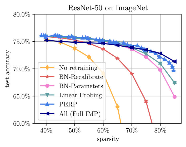
Figure 2: ResNet-50 on ImageNet: Test accuracy across sparsity levels for One Shot pruning with one retraining epoch.

For NLP, we follow Sun et al. (2023) and prune all linear layers except the embedding and final classification head, assigning uniform sparsity to all layers. We provide experiments for unstructured and the semi-structured 2:4 and 4:8 sparsities (Mishra et al., 2021). For vision, we follow Zimmer et al. (2023) and globally prune everything except biases and Batch-Normalization (BN) parameters.

3 Parameter-Efficient Retraining

3.1 Restoring feature quality with few parameters

Pruning can be seen as distorting the initially acquired features, diminishing the network’s expressivity by settling on suboptimal features. With most parameters set to be immutable, our goal is to regain performance (maximizing accuracy or minimizing perplexity) with minimal number of trainable parameters. To that end, we examine subgroups of parameters with varying complexity, which we hypothesize to hold significant expressive power during retraining.

Before introducing the methods we aim to investigate, we note that a significant role in model expressivity is played by normalization layers such as Batch-Normalization (BN) (Ioffe & Szegedy, 2015) and Layer-Normalization (LN) (Ba et al., 2016). Specifically, BN layers standardize the preceding layer’s output and act differently during training and inference. During training, BN calculates the batch mean and variance in an on-the-fly manner. During inference, BN uses running averages of mean and variance from the training phase, adjusting the model to the data distribution.

We begin by investigating the following approaches, which we design to build upon one another, as we will clarify:

• BN-Recalibrate: Li et al. (2020) identified that recalibrating the BN statistics after pruning enhances generalization. This approach entails a one-time evaluation on the training dataset, neither requiring backpropagation nor altering the training set performance.

• Biases: We only retrain the network’s biases. Despite corresponding to only a small fraction of the total parameters, biases are crucial for model expressivity; Zaken et al. (2021) specifically propose a FT method that adjusts only these biases to the new task.

• BN-Parameters: Beyond statistics, BN layers also include trainable scaling and bias parameters. Their importance has been highlighted in transfer learning (Mudrakarta et al., 2018; Giannou et al., 2023) and Frankle et al. (2020) demonstrated that training only these parameters can enable otherwise frozen, randomly-initialized networks to achieve significant accuracy.

• Linear Probing: A commonly used PEFT approach is Linear Probing, where all parameters remain fixed except for the final linear layer (also called head or classifier) to align the existing features to the new task.

We further define each method to build upon the previous one with increasing complexity, i.e., Linear Probing is intended to additionally unfreeze all parameters of preceding methods. To be more precise, let $\mathcal{W}(\mathcal{M})$ represent the parameter set updated under method $\mathcal{M}$, then

$$\mathcal{W}(\textit{BN-Recalibrate}) \subsetneq\mathcal{W}(\textit{Biases})\subsetneq\mathcal{W}(\textit{BN-Parameters})$$

$$\subsetneq\mathcal{W}(\textit{Linear Probing})\subsetneq\mathcal{W}(\textit{IMP}).$$

For clarity, a ResNet-50 has roughly 26 million parameters, with IMP updating all of these. The least complex method, BN-Recalibrate, requires only a forward pass and no gradient computation at all. On the other hand, updating all non-BN biases requires gradients for about 0.004% of the parameters and also updates BN statistics. Including all BN parameters raises this count to 0.21%, while Linear Probing requires around 8.25% of the parameters.

The GPT models utilize LN, which calculates mean and variance consistently during both training and inference, unlike BN. Thus, for these models, we update LN-Parameters instead of BN-Parameters and further exclude the recalibration. Before examining the efficacy of the selective parameter-efficient retraining strategies just presented, we explore the application of the well-known reparametrization approach, LoRA (Hu et al., 2021).

Retraining as Low-Rank Adaption. The motivation for LoRA stems from the observation that pretrained models exhibit low intrinsic dimensionality (Aghajanyan et al., 2020): results comparable to full FT can be achieved even with restricted, low-dimensional reparametrizations. Extending this logic, we hypothesize that pruned networks can be retrained parameter-efficiently through low-rank adaption.

Yet, adapting LoRA to the prune-retrain paradigm poses challenges. In dense models, LoRA does not increase inference costs during deployment since eventually undoing the reparametrization by setting $W\leftarrow W+BA$ and then removing $B$ and $A$ recovers the original architecture. However, for pruning, integrating the dense matrix $BA$ compromises the sparsity of the pruned tensor $W$. While this issue is easy to address for structured sparsity patterns (see Appendix A), we argue that in the unstructured case the overall parameter increase by adding LoRA layers is negligible.

Precisely, in unstructured weight pruning, the matrix $W$ has sparsity scattered throughout, yielding a dispersed pattern of zeros. Instead of merging $BA$ into $W$ after retraining, which would destroy this sparsity, we retain $B$, $A$ and $W$ as separate matrices in the model. The minimal parameter count of $A$ and $B$ barely impacts the model’s size. This addition, however, does decrease the overall sparsity slightly, which we account for in our reporting.

In the following, we use the umbrella term Parameter-Efficient Retraining after Pruning (PERP) for our approach that combines updating biases, normalization parameters, the linear head, and low-rank adaptation of other layers.

Results. In Figure 2, we compare the test accuracy of the methods after One Shot pruning and retraining using ResNet-50 on ImageNet. For clarity, we exclude Biases due to its minimal improvement over BN-Recalibrate. We note that pruning without retraining is unable to maintain performance, even at moderate sparsity. However, recalibrating BN statistics recovers much of the performance at test time, supporting the findings of Li et al. (2020). Surprisingly, BN-Parameters restores most of the performance, nearly matching full retraining with up to 70% of the parameters pruned, while retraining only 0.21% of the architecture’s 26M parameters, thus significantly reducing memory usage.

At moderate sparsity, adjusting only BN parameters can outperform full retraining. We think that this largely aligns with the observation that full FT in transfer learning can harm pretrained (or in our case pruned) features, a problem Kumar et al. (2022a) mitigate by adjusting only the linear head. In Appendix B, we demonstrate that longer retraining addresses this, giving the proposed methods an efficiency advantage when comparing on equal performance terms. Linear Probing further enhances performance in high sparsity scenarios, though it is not fully able to close the gap to full retraining: higher sparsity levels require updating more parameters to counteract pruning-induced performance loss.

Finally, PERP, further incorporating LoRA, significantly narrows the performance gap observed in earlier approaches. We reparametrize all layers except the linear head, see Appendix A for details. Using PERP, the fraction of trainable parameters ranges between 8.6% and 12.5% of the full model, depending on $r$. PERP surpasses previous methods across a wide range of sparsity levels, exceeding IMP until about 75% sparsity. To account for the slight decrease in overall sparsity, Figure 2 plots a broader range of sparsity levels by varying values for the rank $r$ (1, 2, 5, 10).

3.2 Efficient Retraining of Large Models

We demonstrated that only very few parameters are actually needed to restore performance after One Shot pruning ResNet-50. Especially normalization parameters in combination with low-rank adapters are able to adjust the pruned features to work notably well, despite pruning damaging the model and dropping performance drastically at moderate sparsities. As we discuss now, PERP is highly effective in the context of LLMs, where full retraining is infeasible.

In Table 1, we present the final Wikitext perplexity for pruning and retraining OPT-2.7B and OPT-30B for 1000 iterations. When comparing to full IMP, we are restricted to using a model no greater than a mere 2.7 billion parameters, as we are not able to fully retrain larger models due to GPU-memory constraints. We overcome the constraint of batch size 1 by accumulating gradients over multiple steps. For PERP, we set the rank to 16 for each attention matrix, noting that we ablate the LoRA configuration in Appendix C. Our experiments also revealed that retraining the embedding layer was not effective, and retraining the entire linear head, as in Linear Probing, was less stable than applying LoRA reparametrization to it, further minimizing trainable parameters. The resulting reduction in overall sparsity by PERP is a negligible 0.10%-0.19%.

PERP matches Full IMP’s perplexity while only retraining 0.27% of the 2.7 billion parameters, even outperforming it for higher levels of sparsity where the increase in perplexity compared to the dense model is non-negligible. We observe similar differences between the approaches as before, except that Linear Probing often slightly underperforms LN-Parameters. Unlike accuracy, perplexity is unbounded and can explode with increased sparsity, as visible when not performing any retraining. Nevertheless, the perplexity is reduced effectively by PERP. We note that retraining the dense model on C4 does not bring any benefits and that these results transfer to the LLaMa-2, Mistral and Mixtral models, cf. Appendix B.

We highlight that we are able to retrain the 30B parameter model using just a single NVIDIA A100 GPU, underscoring the memory efficiency of PERP in the pruning context. In contrast, full retraining of OPT-30B would require multiple GPUs. However, PERP not only cuts down storage costs and enables retraining of large models, but also enhances retraining efficiency. For instance, using OPT-2.7B on the same compute setup, full retraining achieves a maximum of 3500 train tokens per second (tps), whereas PERP nearly doubles this efficiency to 6400 tps. Updating only biases and normalization parameters further increases this rate to 7600 tps. In addition, as depicted in Figure 3 displaying the perplexity (log-scale) vs. the number of retraining iterations, PERP rapidly decreases the perplexity of OPT-6.7B across various sparsity levels. Without retraining (i.e., zero iterations), perplexity explodes exponentially from approximately $10^{1}$ to $10^{4}$. However, PERP significantly lowers perplexity and saturates after only a few iterations. This efficient retraining is also evident in Figure 2, where a single epoch suffices to restore accuracy at moderate to high sparsity levels, contrasting with the more extensive epoch requirements of full retraining.

In summary, our results demonstrate that updating a critical subset of parameters and applying LoRA suffices to restore a significant portion of the performance achievable through full retraining. This approach not only enables retraining of large models within memory constraints but also ensures efficiency, requiring minimal yet effective iterations for performance recovery. PERP thereby makes the retraining of pruned models feasible, even on constrained hardware resources and with GPT-scale models. In Appendix C, we dissect the impact of the individual methods by comparing all possible combinations of parameter groups.

Table 1: OPT-2.7B/30B: Parameter-efficient approaches vs. full retraining with 30%-70% of the parameters pruned. The first column lists the method, and the second shows the percentage of trainable parameters (Full IMP represents the standard retraining baseline). The next five columns display the average mean perplexity (lower is better) across multiple seeds, with standard deviations excluded for clarity. The dense model attains a perplexity of 12.47 and 9.55 for OPT-2.7B/30B, respectively.

OPT-2.7B
Perplexity: 12.47		Sparsity
Method	% trainable	30%	40%	50%	60%	70%
Full IMP	100%	13.47	14.31	15.85	19.54	28.37
PERP	0.27%	13.42	14.50	16.38	19.20	27.01
Linear Probing	0.07%	13.47	14.71	17.10	21.33	35.75
LN-Parameters	0.04%	13.53	14.71	16.66	21.12	34.39
Biases	0.03%	13.58	14.84	16.86	22.07	39.57
No Retraining	0.00%	15.58	30.32	265.19	3604.16	7251.81
OPT-30B
Perplexity: 9.55		Sparsity
Method	% trainable	30%	40%	50%	60%	70%
PERP	0.09%	10.43	11.42	12.29	14.50	21.66
Linear Probing	0.02%	10.31	11.49	12.80	15.75	54.26
LN-Parameters	0.01%	10.37	11.43	12.82	15.75	43.06
Biases	0.01%	10.41	11.49	13.80	17.00	408.04
No retraining	0.00%	12.37	24.29	168.07	11675.34	28170.72

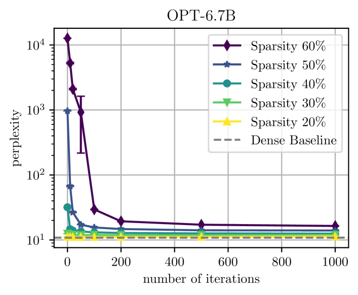
Figure 3: OPT-6.7B evaluated on WikiText: Final perplexity after retraining for as many iterations as indicated on the x-axis. PERP retrains only 0.16% of the parameters.

3.3 Reconsidering Magnitude Pruning of LLMs

The rise of LLMs has rendered classical retraining impractical, as fully retraining GPT-scale models, even in the One Shot case, exceeds the resource capabilities of many practitioners (Jaiswal et al., 2023a). As we have demonstrated, retraining can become much more efficient and viable by focusing on the network’s most critical parameters. At the same time, there is growing interest in developing pruning criteria other than magnitude that yield high-performance models without the need for retraining (Kwon et al., 2022; Frantar & Alistarh, 2023; Sun et al., 2023).

Despite its effectiveness in the domain of convolutional architectures, the magnitude-criterion has been recognized as unsuited for pruning LLMs in a retraining-free setting (Frantar & Alistarh, 2023; Sun et al., 2023). Yin et al. (2023) considered magnitude pruning as no better than random pruning at higher sparsities and note that its success is closely intertwined with the feasibility of retraining. Both Sun et al. (2023) and Yin et al. (2023) explain the inability to magnitude-prune LLMs with observations made by Dettmers et al. (2022) regarding the emergence of large magnitude features in transformers beyond a certain size. These large features, a small yet significant subset of hidden features, are critical for model performance, and pruning them severely impacts predictive accuracy (Sun et al., 2023); a problem that magnitude pruning fails to address.

We agree and have demonstrated that simple magnitude pruning leads to a model collapse at even moderate sparsity, making it unsuitable for a retraining-free scenario. However, our successful mitigation of the exploding perplexity issue with minimal memory requirements suggests revisiting the applicability of magnitude pruning for LLMs, particularly as previous studies report high perplexity and suggest that entirely new pruning criteria are needed for LLMs.

We evaluate magnitude pruning against two state-of-the-art retraining-free pruning methods: SparseGPT (Frantar & Alistarh, 2023) and Wanda (Sun et al., 2023). SparseGPT, using second-order information to address a layer-wise reconstruction problem, prunes large models with little increase in perplexity, however at the price of increased pruning time. Notably, SparseGPT not only identifies a pruning mask but also adjusts the remaining weights to minimize discrepancies between the dense and sparse model. Wanda enhances the magnitude criterion to incorporate the feature activation, reaching performance competitive to SparseGPT in a more efficient way. As opposed to magnitude pruning, both approaches rely on calibration data, which influences the quality of the final result (Williams & Aletras, 2023).

Table 2 presents a comparative analysis of pruning criteria on OPT-2.7B/6.7B/13B/30B models with 50% weight removal and semi-structured 2:4 and 4:8 sparsity. The first row represents the baseline case without pruning. We assess both magnitude pruning with and without PERP. For fairness, we also retrained Wanda and SparseGPT with PERP, listing the full results with and without PERP in the appendix. The appendix further contains results for other models.

As similarly seen in Figure 3, while magnitude pruning substantially increases perplexity, PERP efficiently reduces it to levels on par with SparseGPT and Wanda across all configurations. This indicates that while magnitude pruning alone may be ineffective, it is not inherently unsuited for LLMs despite presumably failing to address large features. Minimal, efficient retraining can significantly recover close to initial perplexity, offering a viable option over completely avoiding retraining. Nevertheless, magnitude pruning with PERP does not entirely match the performance of Wanda and SparseGPT, with the gap reducing as model size increases. This highlights the merit of (and the need for more) precise LLM-pruning methods such as Wanda and SparseGPT. However, given that both require calibration data and a more time-intensive pruning step than the simple magnitude heuristic, we think that practitioners should choose depending on model size and the desired degree of sparsification, where magnitude pruning might be preferable due to its speed advantage, even if it entails some parameter-efficient retraining. Figure 3 also underlines that, in the case of magnitude pruning, the minimum number of retraining iterations to reach good performance directly depends on the impact of compression or goal sparsity at hand, which is not necessarily the case for other methods such as Wanda. Appendix C discusses the setting with higher sparsity levels.

Table 2: OPT-2.7B/6.7B/13B/30B: Perplexity comparison of naive magnitude pruning to magnitude pruning, Wanda and SparseGPT with PERP, both in the unstructured pruning setting (50% sparsity), as well as for the semi-structured 2:4 and 4:8 sparsities. All methods using PERP (indicated in the second column) are retrained for 1000 iterations and further highlighted in bold. We report the mean perplexity over several seeds and omit the standard deviation for the sake of clarity.

			OPT
Method	PERP	Sparsity	2.7B	6.7B	13B	30B
Baseline	✗	0%	12.47	10.86	10.12	9.55
Magnitude	✗	50%	265.19	968.80	11568.33	168.07
Magnitude	✓	50%	15.76	13.60	12.54	11.94
Wanda	✓	50%	13.88	11.83	11.06	10.03
SparseGPT	✓	50%	13.40	11.47	10.85	9.76
Magnitude	✗	2:4	1152.89	264.09	484.74	1979.66
Magnitude	✓	2:4	17.90	14.31	13.14	12.27
Wanda	✓	2:4	16.29	13.48	12.03	10.92
SparseGPT	✓	2:4	15.23	12.70	11.56	10.39
Magnitude	✗	4:8	166.92	196.17	449.64	563.84
Magnitude	✓	4:8	16.43	13.77	12.57	12.06
Wanda	✓	4:8	14.99	12.53	11.41	10.58
SparseGPT	✓	4:8	14.23	11.98	11.03	10.13

3.4 Magnitude conservation: Restabilizing the network

We demonstrated the ability to restore performance efficiently. However, as detailed in Section 2, restoring performance is not the only objective of retraining. For high sparsity levels, employing multiple prune-retrain cycles or phases can be advantageous to avoid layer-collapse, a scenario where a layer is entirely pruned, potentially rendering the model dysfunctional (Tanaka et al., 2020).

While methods like PERP update a subset of parameters or additional ones, they do not inherently prevent layer collapse, as most parameters remain unchanged. An exception is the use of PERP in structured pruning, which allows for updating all non-pruned weights by merging the adapters and pretrained weights at the end of each phase. For unstructured pruning, the challenge is to ensure magnitude conservation by updating all parameters while also being parameter-efficient. Inspired by the transfer learning research of Kumar et al. (2022a, b), we explore the strategy of selectively updating layers based on their role and position in the network. These studies suggest that lower layers require less updating over the course of FT, leading to techniques like gradual unfreezing of the model.

In our ImageNet experiments in Table 12 in the appendix, we test gradual freezing and unfreezing of layers across retraining epochs within a phase, either beginning with the full model and progressively freezing parameters (unfreeze ✗), or starting with a frozen model and gradually unfreezing (unfreeze ✓). Further, we freeze or unfreeze from input to output layer (reverse ✗) or vice-versa (reverse ✓). This process aligns the proportion of layers unfrozen or frozen with the proportion of performed epochs within a phase, ensuring that each parameter is adequately updated, preventing layer collapse while limiting the number of trainable parameters for efficiency. However, unlike previous methods with consistent memory demands throughout epochs, these approaches vary memory requirements and, although they might eventually retrain the entire model, significantly reduce overall memory and computational demands throughout a phase.

We report ImageNet results for varying numbers of phases (2-5), each spanning five epochs, targeting a final sparsity of 90%. The table shows the mean accuracy deviation from full IMP, with standard deviations omitted for clarity. Each of the four variations results in a different total of trainable parameters (aggregated over all epochs in each phase). There is a clear correlation between performance and the fraction of trainable parameters; having 70% of the aggregated trainable parameters is sufficient to achieve results competitive with IMP. We note that in the final phase of IMP, PERP could further reduce these demands. Although these results are encouraging, it is important to note that this approach ultimately involves retraining the entire model, rendering it unsuitable for memory-constrained environments. We believe this area holds promise for future research.

4 Discussion

We demonstrated that retraining a minimal fraction of parameters is sufficient for mitigating pruning-induced performance drops. Our approach can require as little as 0.09% of the parameters used in full IMP, significantly lowering computational and memory demands. This efficiency enables the retraining of LLMs with up to 30 billion parameters on a single NVIDIA A100 within minutes. Our findings make retraining after pruning a viable option for large models and we hope to stimulate further research on both training-free pruning criteria as well as efficient retraining.

Appendix A Technical details and training settings

A.1 Pretraining

Training settings and metrics.

For NLP tasks, we use pretrained models from Huggingface and specify only the retraining settings as outlined in Section 2.3. For computer vision tasks, we perform the pretraining process ourselves. Table 3 details our pretraining configurations, including the number of epochs, batch size, weight decay, and learning rate. We opt for SGD as the optimizer, though we recognize a range of other optimization methods are available (see e.g., Kingma & Ba, 2014; Pokutta et al., 2020). We maintain the default momentum value of 0.9. In the last column of the table we report the performance achieved with standard dense training, using top-1 test accuracy as the metric for image classification tasks, which denotes the percentage of test samples correctly classified.

Table 3: Exact pretraining configurations in our vision experiments.

Dataset	Network (number of weights)	Epochs	Batch size	Weight decay	Learning rate ($t$ = training epoch)	Unpruned test accuracy
ImageNet	ResNet-50 (26 Mio)	90	256	1e-4	linear from 0.1 to 0	76.12% ±0.01%

A.2 Pruning and Retraining

Pruning settings.

Effective pruning relies on the accurate identification of weights to prune and the distribution of sparsity among the layers. Zhu & Gupta (2017) introduced the Uniform allocation, pruning each layer by the same relative amount. Gale et al. (2019) improved this with Uniform+, keeping the first convolutional layer dense and limiting pruning in the final fully-connected layer to 80%. Evci et al. (2020) adapted the Erdős-R’enyi Kernel (ERK) (Mocanu et al., 2018) for layerwise sparsity, accounting for layer dimensions. Lee et al. (2020) proposed Layer-Adaptive Magnitude-based Pruning (LAMP), targeting minimal output distortion at pruning, assessed through $L_{2}$-distortion on worst-case inputs.

In NLP, following Sun et al. (2023), we prune all linear layers except embeddings and the final classification head, applying uniform sparsity throughout. For a comparison of diverse selection schemes for LLMs, see Yin et al. (2023). Our experiments include both unstructured sparsity and semi-structured 2:4 and 4:8 sparsities. In vision tasks, aligning with Zimmer et al. (2023); Evci et al. (2020); Dettmers & Zettlemoyer (2019), we prune everything except biases and BN parameters, employing the Global criterion which treats all parameters as a single vector and computes a universal threshold for parameter removal.

Hyperparameters for Retraining: The Learning Rate.

In computer vision, automating the learning rate schedule for retraining has received increased interest, aiming to circumvent the need for tuning the schedule in each phase. We describe various schedules where $T$ is the total number of epochs of original training with a learning rate schedule $(\eta_{t})_{t\leq T}$, and $T_{{rt}}$ is the number of epochs in each retraining phase. FT (Han et al., 2015) uses a constant learning rate, $\eta_{T}$, from the final epoch of initial training. LRW (Renda et al., 2020) repeats the last $T-T_{{rt}}$ epochs of the original schedule. SLR (Le & Hua, 2021) compresses the initial schedule into the retraining period with an initial warm-up. CLR (Le & Hua, 2021) uses a cosine-based schedule with a warm-up to $\eta_{1}$. LLR (Zimmer et al., 2023) linearly decays from $\eta_{1}$ to zero in each cycle. For vision tasks, we adopt ALLR as recommended by Zimmer et al. (2023), using a linear schedule that adjusts the initial rate based on the impact of pruning and available retraining time, balancing cycle length and pruning-induced performance degradation.

For LLMs, we stick to AdamW with a linear learning rate decay from a tuned initial value. We experiment with starting values 5e-6, 1e-5, 5e-5, 1e-4 and 5e-4.

Hyperparameters for Retraining: Batch size and Weight decay.

For vision, we retain the same batch size and weight decay parameters as used in pretraining. However, for LLMs we set the weight decay to zero and found no improvement in increasing this value. We use a batch size of 2 and gradient accumulation for 4 steps for all models with less than 30 billion parameters. For larger models, we use a batch size of 1 and 2 gradient accumulation steps. We use gradient checkpointing to reduce the memory demands at the expense of efficiency.

LoRA for convolutions and pruned layers.

To apply LoRA to a convolutional tensor $W\in\mathbb{R}^{n\times c\times d\times d}$, with $c$ in-channels, $n$ filters, and spatial size $d$, we view it as an $(n\times cd^{2})$-matrix. As noted in Section 3, we cannot reintegrate the matrix $BA$ into the original weight matrix $W$, as this would destroy the sparsity pattern of $W$. However, this is not necessarily the case for structured pruning.

In the case of convolutional filter pruning, we could simply apply LoRA to the non-pruned segment of the convolutional tensor. Pruning filters equates to zeroing entire rows of $W$. This results in two partitions: $W_{\text{z}}$ for the zeroed rows and $W_{\text{nz}}$ for the rest. LoRA could be applied specifically to the $W_{\text{nz}}$ section, leveraging its smaller size for a concise reparametrization as $W_{\text{nz}}+BA$. During computation, we process $W_{\text{nz}}+B_{\text{nz}}A_{\text{nz}}$ and $W_{\text{z}}$ separately—the latter producing only zeros—and reorder the outputs to match the original row or filter sequence. This reparametrization is easily reversed after retraining, ensuring consistency with the tensor’s original layout. A similar argument can be made for semi-structured sparsities such as 2:4 and 4:8.

Appendix B Additional experiments

In this section, we provide additional results, following the same structure as Section 3.

B.1 Restoring feature quality with few parameters

Figure 4 compares the different approaches on ResNet-50 on ImageNet. As opposed to Figure 2, we perform five retraining epochs instead of a single one.

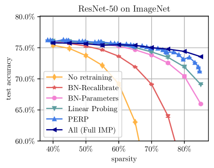
Figure 4: ResNet-50 on ImageNet: Test accuracy across sparsity levels for One Shot pruning with five retraining epochs.

B.2 Efficient Retraining of Large Models

Table 4, Table 5, Table 6, Table 7 and Table 8 shows the full results of the parameter-efficient retraining approaches for OPT, LLaMA-2, Mistral and Mixtral models, which were omitted from the main part of our work. For LLaMA-70B and Mixtral-8x7B, we use a smaller range of sparsities. Note that for all models except the OPT-family, biases are disabled by default and we consequently not include the method Biases.

Table 4: OPT-1.3B/2.7B/13B/30B: Parameter-efficient retraining approaches vs. full retraining with 30%-70% of the parameters pruned. The first column lists the method, and the second shows the percentage of trainable parameters (Full IMP represents the standard retraining baseline). The next five columns display the average mean perplexity (lower is better) across multiple seeds, with standard deviations excluded for clarity. The unpruned model attains a perplexity of 14.62, 12.47, 10.12 and 9.55 for OPT-1.3B/2.7B/13B/30B, respectively.

OPT-1.3B
Perplexity: 14.62		Sparsity
Method	% trainable	30%	40%	50%	60%	70%
Full IMP	100%	15.92	16.94	18.56	23.43	33.60
PERP	0.35%	15.97	16.94	18.60	23.28	34.32
Linear Probing	0.11%	16.01	17.37	19.29	26.00	49.60
LN-Parameters	0.05%	15.91	17.27	19.43	25.91	49.24
Biases	0.03%	16.05	17.60	20.21	28.21	62.03
No Retraining	0.00%	24.74	387.76	1713.30	9390.83	9441.80
OPT-2.7B
Perplexity: 12.47		Sparsity
Method	% trainable	30%	40%	50%	60%	70%
Full IMP	100%	13.47	14.31	15.85	19.54	28.37
PERP	0.27%	13.42	14.50	16.38	19.20	27.01
Linear Probing	0.07%	13.47	14.71	17.10	21.33	35.75
LN-Parameters	0.04%	13.53	14.71	16.66	21.12	34.39
Biases	0.03%	13.58	14.84	16.86	22.07	39.57
No Retraining	0.00%	15.58	30.32	265.19	3604.16	7251.81
OPT-13B
Perplexity: 10.12		Sparsity
Method	% trainable	30%	40%	50%	60%	70%
PERP	0.13%	10.91	11.79	13.29	14.81	18.70
Linear Probing	0.03%	10.94	11.88	13.43	15.83	21.02
LN-Parameters	0.02%	10.87	11.79	13.41	15.75	20.89
Biases	0.01%	11.02	11.88	13.63	16.48	23.68
No retraining	0.00%	13.40	99.26	11591.62	576372.38	290838.78
OPT-30B
Perplexity: 9.55		Sparsity
Method	% trainable	30%	40%	50%	60%	70%
PERP	0.09%	10.43	11.42	12.29	14.50	21.66
Linear Probing	0.02%	10.31	11.49	12.80	15.75	54.26
LN-Parameters	0.01%	10.37	11.43	12.82	15.75	43.06
Biases	0.01%	10.41	11.49	13.80	17.00	408.04
No retraining	0.00%	12.37	24.29	168.07	11675.34	28170.72

Table 5: LLaMA-7B/13B: Parameter-efficient retraining approaches with 30%-70% of the parameters pruned. The first column lists the method, and the second shows the percentage of trainable parameters. The next five columns display the average mean perplexity (lower is better) across multiple seeds, with standard deviations excluded for clarity. The unpruned model attains a perplexity of 5.11, 4.57 for LLaMA-7B/13B, respectively.

LLaMA-7B
Perplexity: 5.11		Sparsity
Method	% trainable	30%	40%	50%	60%	70%
PERP	0.60%	5.35	5.67	6.32	7.62	10.60
Linear Probing	0.01%	5.43	5.89	6.90	9.62	20.45
LN-Parameters	0.00%	5.48	5.98	7.57	10.53	47.58
No retraining	0.00%	5.79	7.31	14.90	3677.83	52432.10
LLaMA-13B
Perplexity: 4.57		Sparsity
Method	% trainable	30%	40%	50%	60%	70%
PERP	0.49%	4.75	4.97	5.42	6.38	8.62
Linear Probing	0.01%	4.77	5.04	5.64	7.28	11.31
LN-Parameters	0.00%	4.77	5.05	5.65	7.33	11.42
No retraining	0.00%	4.82	5.26	6.37	11.22	275.20

Table 6: LLaMA-70B: Parameter-efficient retraining approaches with 40%-60% of the parameters pruned. The first column lists the method, and the second shows the percentage of trainable parameters. The next five columns display the average mean perplexity (lower is better) and standard deviation across multiple seeds. The unpruned model attains a perplexity of 3.12.

LLaMA-70B
Perplexity: 3.12		Sparsity
Method	% trainable	40%	50%	60%
PERP	0.30%	3.49 ±0.00	3.89 ±0.00	4.57 ±0.00
Linear Probing	0.00%	3.54 ±0.00	4.01 ±0.00	4.83 ±0.01
LN-Parameters	0.00%	3.54 ±0.00	4.04 ±0.00	4.95 ±0.01
No retraining	0.00%	3.84 ±0.00	4.99 ±0.00	8.20 ±0.00

Table 7: Mistral-7B: Parameter-efficient retraining approaches with 30%-70% of the parameters pruned. The first column lists the method, and the second shows the percentage of trainable parameters. The next five columns display the average mean perplexity (lower is better) across multiple seeds, with standard deviations excluded for clarity. The unpruned model attains a perplexity of 4.69.

Mistral-7B
Perplexity: 4.69		Sparsity
Method	% trainable	30%	40%	50%	60%	70%
PERP	0.59%	4.95	5.24	5.88	7.63	12.64
Linear Probing	0.01%	5.00	5.46	6.85	16.70	25071.97
LN-Parameters	0.00%	4.98	5.45	6.99	20.42	24993.66
No retraining	0.00%	5.02	5.55	7.92	224.22	68142.05

Table 8: Mixtral-8x7B: Parameter-efficient retraining approaches with 40%-60% of the parameters pruned. The first column lists the method, and the second shows the percentage of trainable parameters. The next five columns display the average mean perplexity (lower is better) and standard deviation across multiple seeds. The unpruned model attains a perplexity of 3.35.

Mixtral-8x7B
Perplexity: 3.35		Sparsity
Method	% trainable	40%	50%	60%
PERP	0.03%	4.04 ±0.00	4.59 ±0.01	5.79 ±0.02
Linear Probing	0.00%	4.56 ±0.00	6.16 ±0.01	19.39 ±0.25
LN-Parameters	0.00%	4.57 ±0.00	6.29 ±0.00	18.83 ±0.06
No retraining	0.00%	4.88 ±0.00	8.30 ±0.00	77.09 ±0.00

B.3 Reconsidering Magnitude Pruning of LLMs

Table 9 and Table 10 show the full results when comparing magnitude pruning, Wanda and SparseGPT with or without PERP on OPT-2.7B/6.7B/13B/30B/66B, LLaMA-7B/13B and Mistral-7B. Surprisingly, for OPT-66B, we see slightly different behaviour then on OPT-30B: magnitude pruning with PERP is able to outperform Wanda with PERP in certain setting. On the other hand, we note that there exist settings where Wanda has higher perplexity than Magnitude when not performing retraining, but outperforming it after retraining. Table 11 compares the final accuracy of these methods on the EleutherAI evaluation set, consisting of seven different tasks, namely: BoolQ (Clark et al., 2019), RTE (Wang et al., 2018), HellaSwag (Zellers et al., 2019), WinoGrande (Sakaguchi et al., 2021), ARC Easy, ARC Challenge (Clark et al., 2018), and OpenbookQA (Mihaylov et al., 2018). We report the mean accuracy over these tasks. The central observation is here that PERP is able to improve the accuracy of the pruning approaches in all cases.

Table 9: OPT-2.7B/6.7B/13B/30B/66B: Perplexity comparison of magnitude pruning, Wanda and SparseGPT, either with our without PERP, both in the unstructured pruning setting (50% sparsity), as well as for the semi-structured 2:4 and 4:8 sparsities. All methods using PERP (indicated in the second column) are retrained for 1000 iterations and further highlighted in bold. We report the mean perplexity over several seeds and omit the standard deviation for the sake of clarity.

			OPT
Method	PERP	Sparsity	2.7B	6.7B	13B	30B	66B
Baseline	✗	0%	12.47	10.86	10.12	9.55	9.33
Magnitude	✗	50%	265.19	968.80	11568.33	168.07	4230.77
Magnitude	✓	50%	15.76	13.60	12.54	11.94	12.17
Wanda	✗	50%	14.35	12.04	11.98	10.07	3730.34
Wanda	✓	50%	13.88	11.83	11.06	10.04	13.91
SparseGPT	✗	50%	13.47	11.59	11.22	9.78	9.32
SparseGPT	✓	50%	13.40	11.47	10.85	9.76	9.41
Magnitude	✗	2:4	1152.89	264.09	484.74	1979.66	6934.42
Magnitude	✓	2:4	17.90	14.31	13.14	12.27	49.58
Wanda	✗	2:4	21.33	16.03	15.70	13.26	11703.72
Wanda	✓	2:4	16.29	13.48	12.03	10.92	19.58
SparseGPT	✗	2:4	17.26	14.23	12.92	10.94	10.13
SparseGPT	✓	2:4	15.23	12.70	11.56	10.39	9.91
Magnitude	✗	4:8	166.92	196.17	449.64	563.84	6736.84
Magnitude	✓	4:8	16.43	13.77	12.57	12.06	20.34
Wanda	✗	4:8	16.85	13.63	13.47	10.88	8743.59
Wanda	✓	4:8	14.99	12.53	11.41	10.58	16.87
SparseGPT	✗	4:8	15.08	12.62	11.80	10.34	9.64
SparseGPT	✓	4:8	14.23	11.98	11.03	10.13	9.62

Table 10: LLaMA-7B/13B and Mistral-7B: Perplexity comparison of magnitude pruning, Wanda and SparseGPT, either with our without PERP, both in the unstructured pruning setting (50% sparsity), as well as for the semi-structured 2:4 and 4:8 sparsities. All methods using PERP (indicated in the second column) are retrained for 1000 iterations and further highlighted in bold. We report the mean perplexity over several seeds and omit the standard deviation for the sake of clarity.

			LLaMA		Mistral
Method	PERP	Sparsity	7B	13B	7B
Baseline	✗	0%	5.11	4.57	4.69
Magnitude	✗	50%	14.90	6.37	7.92
Magnitude	✓	50%	6.32	5.42	5.82
Wanda	✗	50%	6.46	5.59	6.16
Wanda	✓	50%	6.02	5.31	5.46
SparseGPT	✗	50%	6.52	5.64	6.09
SparseGPT	✓	50%	6.04	5.33	5.56
Magnitude	✗	2:4	54.39	8.32	22.63
Magnitude	✓	2:4	7.46	6.29	7.70
Wanda	✗	2:4	11.36	8.35	12.24
Wanda	✓	2:4	7.17	6.18	6.58
SparseGPT	✗	2:4	10.22	8.26	10.12
SparseGPT	✓	2:4	7.09	6.18	6.78
Magnitude	✗	4:8	16.53	6.76	10.82
Magnitude	✓	4:8	6.83	5.81	6.82
Wanda	✗	4:8	8.07	6.55	7.90
Wanda	✓	4:8	6.57	5.77	6.01
SparseGPT	✗	4:8	7.93	6.55	7.84
SparseGPT	✓	4:8	6.54	5.74	6.15

Table 11: OPT-2.7B/6.7B/13B/30B: Accuracy comparison on the EleutherAI evaluation set. We report magnitude pruning, Wanda and SparseGPT, either with our without PERP, both in the unstructured pruning setting (50% sparsity), as well as for the semi-structured 2:4 and 4:8 sparsities. All methods using PERP (indicated in the second column) are retrained for 1000 iterations and further highlighted in bold. We report the mean accuracy over 7 tasks and over several seeds, omitting the standard deviation for the sake of clarity. Note that as opposed to the perplexity metric, higher accuracy is better.

			OPT
Method	PERP	Sparsity	2.7B	6.7B	13B	30B
Magnitude	✗	50%	40.07%	35.56%	33.68%	36.45%
Magnitude	✓	50%	45.35%	49.81%	50.67%	52.14%
Wanda	✗	50%	45.72%	49.10%	51.24%	53.47%
Wanda	✓	50%	46.99%	50.38%	51.68%	53.76%
SparseGPT	✗	50%	46.73%	50.23%	51.37%	54.25%
SparseGPT	✓	50%	47.22%	51.04%	52.04%	54.26%
Magnitude	✗	2:4	35.83%	36.33%	36.60%	34.90%
Magnitude	✓	2:4	44.25%	48.53%	49.66%	49.23%
Wanda	✗	2:4	42.85%	46.14%	47.66%	49.32%
Wanda	✓	2:4	45.14%	48.89%	50.26%	51.92%
SparseGPT	✗	2:4	43.83%	47.01%	49.08%	51.04%
SparseGPT	✓	2:4	45.55%	49.06%	51.02%	52.78%
Magnitude	✗	4:8	36.97%	36.91%	36.09%	36.92%
Magnitude	✓	4:8	44.34%	49.55%	50.27%	51.73%
Wanda	✗	4:8	43.90%	47.49%	49.13%	51.39%
Wanda	✓	4:8	46.02%	49.52%	50.77%	53.25%
SparseGPT	✗	4:8	45.41%	48.20%	50.24%	52.59%
SparseGPT	✓	4:8	46.98%	50.26%	51.56%	53.55%

B.4 Magnitude conservation: Restabilizing the network

Table 12: ResNet-50 on ImageNet: Iterative parameter-efficient retraining targeting 90% sparsity, with 2 to 5 prune-retrain cycles. The first two columns indicate whether we freeze (✗) or unfreeze (✓) the model during each cycle, and the direction of this process (output-to-input (✓) or input-to-output (✗)). The third column shows the total aggregated percentage of trainable parameters. The subsequent four columns present the average mean test accuracy deviation from full IMP across various seeds, omitting standard deviations for brevity.

ImageNet
			# Prune-Retrain cycles
unfreeze	reverse	% agg. trainable	2	3	4	5
✓	✓	88.83%	-0.27%	-0.09%	-0.07%	-0.46%
✗	✗	70.95%	-1.07%	-0.67%	-0.66%	-0.91%
✓	✗	37.28%	-2.47%	-2.28%	-1.91%	-2.02%
✗	✓	19.40%	-7.16%	-6.98%	-6.67%	-6.59%

Appendix C Ablation studies

C.1 Ablation: Dissecting the impact of parameter groups for LLMs

In Table 13, we analyze the effect of different parameter groups when retraining OPT-13B, magnitude-pruned to 50% and 70% sparsity, for 1000 iterations. We tuned the learning rate and report the best mean perplexity across multiple random seeds, along with the standard deviation. The last two columns show the proportion of trainable parameters and final test perplexity, respectively. The first four columns indicate whether individual parameter groups are active (✓) or inactive (✗), specifically Biases (excluding LN-biases), LN parameters, the linear head, and added LoRA parameters.

Our findings include several key points. Retraining solely the linear head, though significantly reducing perplexity, is outperformed by other methods. LoRA, representing the largest set of trainable parameters, most effectively lowers perplexity. However, retraining biases or LN parameters also notably decreases perplexity, utilizing far fewer parameters than LoRA. Combining all methods typically delivers the best outcomes, with Biases and LN showing diminishing returns. While the linear head alone is less efficient, it aids in further perplexity reduction. Biases and LN parameters are impactful given their minimal parameter count; for optimal performance, we suggest employing all highlighted parameter groups.

Table 13: OPT-13B: The subtables report One Shot parameter-efficient retraining for 50% (above) and 70% (below) sparsity levels. The first four columns specify whether certain model parameter subgroups are inactive (✗) or active (✓), representing the training of (non-LN) biases, Layernorm parameters, the linear head, and low-rank adapters, respectively. The penultimate column presents the percentage of trainable parameters in each configuration. The final column displays the mean perplexity across seeds and its standard deviation.

50%
Biases	LN	Head	LoRA	% trainable	Perplexity
✗	✗	✗	✗	0.00%	11591.62 ±0.00
✓	✗	✗	✗	0.01%	13.66 ±0.01
✗	✓	✗	✗	0.01%	13.88 ±0.05
✗	✗	✓	✗	0.01%	3749.34 ±7.34
✗	✗	✗	✓	0.41%	12.59 ±0.08
✓	✓	✗	✗	0.02%	13.36 ±0.00
✓	✗	✓	✗	0.02%	13.70 ±0.01
✓	✗	✗	✓	0.42%	12.65 ±0.05
✗	✓	✓	✗	0.01%	14.04 ±0.03
✗	✓	✗	✓	0.41%	12.65 ±0.05
✗	✗	✓	✓	0.41%	12.64 ±0.01
✓	✓	✓	✗	0.03%	13.50 ±0.03
✓	✓	✗	✓	0.43%	12.76 ±0.05
✓	✗	✓	✓	0.43%	12.69 ±0.04
✗	✓	✓	✓	0.42%	12.66 ±0.09
✓	✓	✓	✓	0.43%	12.70 ±0.03
70%
Biases	LN	Head	LoRA	% trainable	Perplexity
✗	✗	✗	✗	0.00%	290838.78 ±0.00
✓	✗	✗	✗	0.01%	24.92 ±0.09
✗	✓	✗	✗	0.01%	47.62 ±9.05
✗	✗	✓	✗	0.01%	9413.92 ±134.20
✗	✗	✗	✓	0.41%	17.60 ±0.02
✓	✓	✗	✗	0.02%	22.28 ±0.69
✓	✗	✓	✗	0.02%	25.59 ±1.52
✓	✗	✗	✓	0.42%	17.60 ±0.02
✗	✓	✓	✗	0.01%	93.26 ±77.07
✗	✓	✗	✓	0.41%	17.56 ±0.17
✗	✗	✓	✓	0.41%	17.53 ±0.10
✓	✓	✓	✗	0.03%	21.81 ±0.39
✓	✓	✗	✓	0.43%	17.65 ±0.02
✓	✗	✓	✓	0.43%	18.10 ±0.68
✗	✓	✓	✓	0.42%	17.65 ±0.03
✓	✓	✓	✓	0.43%	17.37 ±0.13

C.2 Ablation: The impact of LoRA hyperparameters

As opposed to methods that activate specific parameter groups, LoRA adds new trainable parameters and two hyperparameters: rank $r$ and scaling factor $\alpha$ (Hu et al., 2021). We investigate how $r$ and $\alpha$ affect retraining pruned models using LoRA. Table 14 shows perplexity results following PERP retraining of 50% pruned OPT-13B. Notably, variations in $r$ and $\alpha$ seem to have minimal impact on final perplexity, even though rank directly affects the number of trainable parameters. We adjusted the learning rate schedule and the number of training iterations (between 100 and 500) and report the best mean perplexity across multiple random seeds.

Table 14: OPT-13B: Perplexity comparison of magnitude pruning with PERP in the unstructured pruning setting (50% sparsity), varying the LoRA rank $r$ and scaling factor $\alpha$ as indicated. We tune the retraining length (100 and 500 iterations) and the learning rate schedule, reporting the best mean perplexity across multiple seeds, including the standard deviation.

	Rank $r$
$\alpha$	8	16	32	64	128
32	12.91 ±0.02	12.86 ±0.07	12.86 ±0.01	12.92 ±0.00	13.10 ±0.03
64	12.78 ±0.12	12.77 ±0.08	12.84 ±0.06	12.84 ±0.11	12.95 ±0.02
128	12.89 ±0.01	12.78 ±0.09	12.92 ±0.02	12.83 ±0.20	12.91 ±0.09

C.3 Ablation: The high sparsity regime

Table 15 examines the perplexity results for unstructured pruning on OPT-30B using magnitude pruning, Wanda, and SparseGPT, both with and without PERP retraining. This table focuses on higher sparsity levels to explore whether our findings extend beyond the 50% threshold. Analyzing the results, all methods significantly benefit from PERP retraining. However, in the extreme sparsity regime (80%), SparseGPT alone maintains reasonable test perplexity. Surprisingly, at higher sparsity levels, magnitude pruning outperforms Wanda after retraining, though this is not the case without retraining.

Table 15: OPT-30B: Perplexity comparison of magnitude pruning, Wanda, and SparseGPT, either with or without PERP in the unstructured pruning setting (50% sparsity). All methods using PERP (indicated in the second column) are retrained for 500 iterations and further highlighted in bold. We report the mean perplexity over several seeds and omit the standard deviation for the sake of clarity.

		Sparsity
Method	PERP	50%	60%	70%	80%
Magnitude	✗	168.07	11677.30	28183.30	56369.09
Magnitude	✓	11.88	14.20	19.01	165.30
Wanda	✗	10.07	26.36	10376.56	7816.61
Wanda	✓	10.06	11.31	29.44	487.80
SparseGPT	✗	9.79	10.71	13.55	46.39
SparseGPT	✓	9.80	10.43	11.83	20.20

References

- Aghajanyan et al. (2020) Aghajanyan, A., Zettlemoyer, L., and Gupta, S. Intrinsic dimensionality explains the effectiveness of language model fine-tuning. December 2020.
- Ba et al. (2016) Ba, J. L., Kiros, J. R., and Hinton, G. E. Layer normalization. July 2016.
- Clark et al. (2019) Clark, C., Lee, K., Chang, M.-W., Kwiatkowski, T., Collins, M., and Toutanova, K. Boolq: Exploring the surprising difficulty of natural yes/no questions. May 2019.
- Clark et al. (2018) Clark, P., Cowhey, I., Etzioni, O., Khot, T., Sabharwal, A., Schoenick, C., and Tafjord, O. Think you have solved question answering? try arc, the ai2 reasoning challenge. March 2018.
- Dettmers & Zettlemoyer (2019) Dettmers, T. and Zettlemoyer, L. Sparse networks from scratch: Faster training without losing performance. arXiv preprint arXiv:1907.04840, July 2019.
- Dettmers et al. (2022) Dettmers, T., Lewis, M., Belkada, Y., and Zettlemoyer, L. Llm.int8(): 8-bit matrix multiplication for transformers at scale. August 2022.
- Ding et al. (2019) Ding, X., Ding, G., Zhou, X., Guo, Y., Han, J., and Liu, J. Global sparse momentum sgd for pruning very deep neural networks. In Wallach, H., Larochelle, H., Beygelzimer, A., d'Alché-Buc, F., Fox, E., and Garnett, R. (eds.), Advances in Neural Information Processing Systems, volume 32. Curran Associates, Inc., 2019. URL https://proceedings.neurips.cc/paper/2019/file/f34185c4ca5d58e781d4f14173d41e5d-Paper.pdf.
- Evci et al. (2020) Evci, U., Gale, T., Menick, J., Castro, P. S., and Elsen, E. Rigging the lottery: Making all tickets winners. In III, H. D. and Singh, A. (eds.), Proceedings of the 37th International Conference on Machine Learning, volume 119 of Proceedings of Machine Learning Research, pp. 2943–2952. PMLR, 13–18 Jul 2020. URL https://proceedings.mlr.press/v119/evci20a.html.
- Evci et al. (2022) Evci, U., Dumoulin, V., Larochelle, H., and Mozer, M. C. Head2toe: Utilizing intermediate representations for better transfer learning. ICML 2022, Proceedings of the 39th International Conference on Machine Learning, January 2022.
- Frankle & Carbin (2018) Frankle, J. and Carbin, M. The lottery ticket hypothesis: Finding sparse, trainable neural networks. In International Conference on Learning Representations, 2018.
- Frankle et al. (2020) Frankle, J., Schwab, D. J., and Morcos, A. S. Training batchnorm and only batchnorm: On the expressive power of random features in cnns. February 2020.
- Frantar & Alistarh (2023) Frantar, E. and Alistarh, D. Sparsegpt: Massive language models can be accurately pruned in one-shot. In International Conference on Machine Learning, pp. 10323–10337. PMLR, 2023.
- Gale et al. (2019) Gale, T., Elsen, E., and Hooker, S. The state of sparsity in deep neural networks. arXiv preprint arXiv:1902.09574, 2019.
- Gao et al. (2023) Gao, L., Tow, J., Abbasi, B., Biderman, S., Black, S., DiPofi, A., Foster, C., Golding, L., Hsu, J., Le Noac’h, A., Li, H., McDonell, K., Muennighoff, N., Ociepa, C., Phang, J., Reynolds, L., Schoelkopf, H., Skowron, A., Sutawika, L., Tang, E., Thite, A., Wang, B., Wang, K., and Zou, A. A framework for few-shot language model evaluation, 12 2023. URL https://zenodo.org/records/10256836.
- Giannou et al. (2023) Giannou, A., Rajput, S., and Papailiopoulos, D. The expressive power of tuning only the normalization layers. February 2023.
- Han et al. (2015) Han, S., Pool, J., Tran, J., and Dally, W. Learning both weights and connections for efficient neural networks. In Cortes, C., Lawrence, N., Lee, D., Sugiyama, M., and Garnett, R. (eds.), Advances in Neural Information Processing Systems, volume 28. Curran Associates, Inc., 2015. URL https://proceedings.neurips.cc/paper/2015/file/ae0eb3eed39d2bcef4622b2499a05fe6-Paper.pdf.
- Hassibi & Stork (1993) Hassibi, B. and Stork, D. Second order derivatives for network pruning: Optimal brain surgeon. In Hanson, S., Cowan, J., and Giles, C. (eds.), Advances in Neural Information Processing Systems, volume 5. Morgan-Kaufmann, 1993. URL https://proceedings.neurips.cc/paper/1992/file/303ed4c69846ab36c2904d3ba8573050-Paper.pdf.
- He et al. (2015) He, K., Zhang, X., Ren, S., and Sun, J. Delving deep into rectifiers: Surpassing human-level performance on imagenet classification. In Proceedings of the IEEE International Conference on Computer Vision (ICCV), December 2015.
- He et al. (2022) He, S., Ding, L., Dong, D., Zhang, M., and Tao, D. Sparseadapter: An easy approach for improving the parameter-efficiency of adapters. October 2022.
- Hoefler et al. (2021) Hoefler, T., Alistarh, D., Ben-Nun, T., Dryden, N., and Peste, A. Sparsity in deep learning: Pruning and growth for efficient inference and training in neural networks. arXiv preprint arXiv:2102.00554, January 2021.
- Houlsby et al. (2019) Houlsby, N., Giurgiu, A., Jastrzebski, S., Morrone, B., De Laroussilhe, Q., Gesmundo, A., Attariyan, M., and Gelly, S. Parameter-efficient transfer learning for nlp. In International Conference on Machine Learning, pp. 2790–2799. PMLR, 2019.
- Hu et al. (2021) Hu, E. J., Shen, Y., Wallis, P., Allen-Zhu, Z., Li, Y., Wang, S., Wang, L., and Chen, W. Lora: Low-rank adaptation of large language models. June 2021.
- Ioffe & Szegedy (2015) Ioffe, S. and Szegedy, C. Batch normalization: Accelerating deep network training by reducing internal covariate shift. In Bach, F. R. and Blei, D. M. (eds.), Proceedings of the 32nd International Conference on Machine Learning, ICML 2015, Lille, France, 6-11 July 2015, volume 37 of JMLR Workshop and Conference Proceedings, pp. 448–456. JMLR.org, 2015. URL http://proceedings.mlr.press/v37/ioffe15.html.
- Jaiswal et al. (2023a) Jaiswal, A., Gan, Z., Du, X., Zhang, B., Wang, Z., and Yang, Y. Compressing llms: The truth is rarely pure and never simple. October 2023a.
- Jaiswal et al. (2023b) Jaiswal, A. K., Liu, S., Chen, T., Ding, Y., and Wang, Z. Instant soup: Cheap pruning ensembles in a single pass can draw lottery tickets from large models. In International Conference on Machine Learning, pp. 14691–14701. PMLR, 2023b.
- Jiang et al. (2023) Jiang, A. Q., Sablayrolles, A., Mensch, A., Bamford, C., Chaplot, D. S., de las Casas, D., Bressand, F., Lengyel, G., Lample, G., Saulnier, L., Lavaud, L. R., Lachaux, M.-A., Stock, P., Scao, T. L., Lavril, T., Wang, T., Lacroix, T., and Sayed, W. E. Mistral 7b. October 2023.
- Kingma & Ba (2014) Kingma, D. P. and Ba, J. Adam: A method for stochastic optimization. arXiv preprint arXiv:1412.6980, 2014.
- Krizhevsky et al. (2012) Krizhevsky, A., Sutskever, I., and Hinton, G. E. Imagenet classification with deep convolutional neural networks. In Pereira, F., Burges, C., Bottou, L., and Weinberger, K. (eds.), Advances in Neural Information Processing Systems, volume 25. Curran Associates, Inc., 2012. URL https://proceedings.neurips.cc/paper_files/paper/2012/file/c399862d3b9d6b76c8436e924a68c45b-Paper.pdf.
- Kumar et al. (2022a) Kumar, A., Raghunathan, A., Jones, R., Ma, T., and Liang, P. Fine-tuning can distort pretrained features and underperform out-of-distribution. February 2022a.
- Kumar et al. (2022b) Kumar, A., Shen, R., Bubeck, S., and Gunasekar, S. How to fine-tune vision models with sgd. November 2022b.
- Kwon et al. (2022) Kwon, W., Kim, S., Mahoney, M. W., Hassoun, J., Keutzer, K., and Gholami, A. A fast post-training pruning framework for transformers. March 2022.
- Le & Hua (2021) Le, D. H. and Hua, B.-S. Network pruning that matters: A case study on retraining variants. In International Conference on Learning Representations, 2021. URL https://openreview.net/forum?id=Cb54AMqHQFP.
- LeCun et al. (1989) LeCun, Y., Denker, J. S., and Solla, S. A. Optimal brain damage. In Touretzky, D. S. (ed.), Advances in Neural Information Processing Systems 2, [NIPS Conference, Denver, Colorado, USA, November 27-30, 1989], pp. 598–605. Morgan Kaufmann, 1989. URL http://papers.nips.cc/paper/250-optimal-brain-damage.
- Lee et al. (2020) Lee, J., Park, S., Mo, S., Ahn, S., and Shin, J. Layer-adaptive sparsity for the magnitude-based pruning. In International Conference on Learning Representations, October 2020.
- Li et al. (2020) Li, B., Wu, B., Su, J., and Wang, G. Eagleeye: Fast sub-net evaluation for efficient neural network pruning. In Computer Vision–ECCV 2020: 16th European Conference, Glasgow, UK, August 23–28, 2020, Proceedings, Part II 16, pp. 639–654. Springer, 2020.
- Li et al. (2022) Li, Y., Luo, F., Tan, C., Wang, M., Huang, S., Li, S., and Bai, J. Parameter-efficient sparsity for large language models fine-tuning. May 2022.
- Lialin et al. (2023a) Lialin, V., Deshpande, V., and Rumshisky, A. Scaling down to scale up: A guide to parameter-efficient fine-tuning. March 2023a.
- Lialin et al. (2023b) Lialin, V., Shivagunde, N., Muckatira, S., and Rumshisky, A. Stack more layers differently: High-rank training through low-rank updates. July 2023b.
- Lin et al. (2020) Lin, T., Stich, S. U., Barba, L., Dmitriev, D., and Jaggi, M. Dynamic model pruning with feedback. In International Conference on Learning Representations, 2020.
- Liu et al. (2021) Liu, B., Cai, Y., Guo, Y., and Chen, X. Transtailor: Pruning the pre-trained model for improved transfer learning. March 2021.
- Liu et al. (2020) Liu, J., Xu, Z., Shi, R., Cheung, R. C. C., and So, H. K. Dynamic sparse training: Find efficient sparse network from scratch with trainable masked layers. In International Conference on Learning Representations, 2020. URL https://openreview.net/forum?id=SJlbGJrtDB.
- Loshchilov & Hutter (2019) Loshchilov, I. and Hutter, F. Decoupled weight decay regularization. In International Conference on Learning Representations, 2019.
- Merity et al. (2016) Merity, S., Xiong, C., Bradbury, J., and Socher, R. Pointer sentinel mixture models. September 2016.
- Mihaylov et al. (2018) Mihaylov, T., Clark, P., Khot, T., and Sabharwal, A. Can a suit of armor conduct electricity? a new dataset for open book question answering. September 2018.
- Mishra et al. (2021) Mishra, A., Latorre, J. A., Pool, J., Stosic, D., Stosic, D., Venkatesh, G., Yu, C., and Micikevicius, P. Accelerating sparse deep neural networks. April 2021.
- Mistral (2023) Mistral, M. A. Mixtral of experts — mistral.ai. https://mistral.ai/news/mixtral-of-experts/, 2023. [Accessed 31-01-2024].
- Mocanu et al. (2018) Mocanu, D. C., Mocanu, E., Stone, P., Nguyen, P. H., Gibescu, M., and Liotta, A. Scalable training of artificial neural networks with adaptive sparse connectivity inspired by network science. Nature Communications, 9(1), June 2018. doi: 10.1038/s41467-018-04316-3.
- Molchanov et al. (2016) Molchanov, P., Tyree, S., Karras, T., Aila, T., and Kautz, J. Pruning convolutional neural networks for resource efficient inference. November 2016.
- Mudrakarta et al. (2018) Mudrakarta, P. K., Sandler, M., Zhmoginov, A., and Howard, A. K for the price of 1: Parameter-efficient multi-task and transfer learning. October 2018.
- Pokutta et al. (2020) Pokutta, S., Spiegel, C., and Zimmer, M. Deep neural network training with frank-wolfe. arXiv preprint arXiv:2010.07243, 2020.
- Raffel et al. (2020) Raffel, C., Shazeer, N., Roberts, A., Lee, K., Narang, S., Matena, M., Zhou, Y., Li, W., and Liu, P. J. Exploring the limits of transfer learning with a unified text-to-text transformer. The Journal of Machine Learning Research, 21(1):5485–5551, 2020.
- Renda et al. (2020) Renda, A., Frankle, J., and Carbin, M. Comparing rewinding and fine-tuning in neural network pruning. In International Conference on Learning Representations, 2020.
- Russakovsky et al. (2015) Russakovsky, O., Deng, J., Su, H., Krause, J., Satheesh, S., Ma, S., Huang, Z., Karpathy, A., Khosla, A., Bernstein, M., Berg, A. C., and Fei-Fei, L. ImageNet Large Scale Visual Recognition Challenge. International Journal of Computer Vision (IJCV), 115(3):211–252, 2015. doi: 10.1007/s11263-015-0816-y.
- Sakaguchi et al. (2021) Sakaguchi, K., Bras, R. L., Bhagavatula, C., and Choi, Y. Winogrande: An adversarial winograd schema challenge at scale. Communications of the ACM, 64(9):99–106, 2021.
- Sun et al. (2023) Sun, M., Liu, Z., Bair, A., and Kolter, J. Z. A simple and effective pruning approach for large language models. June 2023.
- Tanaka et al. (2020) Tanaka, H., Kunin, D., Yamins, D. L. K., and Ganguli, S. Pruning neural networks without any data by iteratively conserving synaptic flow. Advances in Neural Information Processing Systems 2020, June 2020.
- Touvron et al. (2023) Touvron, H., Martin, L., Stone, K., Albert, P., Almahairi, A., Babaei, Y., Bashlykov, N., Batra, S., Bhargava, P., Bhosale, S., Bikel, D., Blecher, L., Ferrer, C. C., Chen, M., Cucurull, G., Esiobu, D., Fernandes, J., Fu, J., Fu, W., Fuller, B., Gao, C., Goswami, V., Goyal, N., Hartshorn, A., Hosseini, S., Hou, R., Inan, H., Kardas, M., Kerkez, V., Khabsa, M., Kloumann, I., Korenev, A., Koura, P. S., Lachaux, M.-A., Lavril, T., Lee, J., Liskovich, D., Lu, Y., Mao, Y., Martinet, X., Mihaylov, T., Mishra, P., Molybog, I., Nie, Y., Poulton, A., Reizenstein, J., Rungta, R., Saladi, K., Schelten, A., Silva, R., Smith, E. M., Subramanian, R., Tan, X. E., Tang, B., Taylor, R., Williams, A., Kuan, J. X., Xu, P., Yan, Z., Zarov, I., Zhang, Y., Fan, A., Kambadur, M., Narang, S., Rodriguez, A., Stojnic, R., Edunov, S., and Scialom, T. Llama 2: Open foundation and fine-tuned chat models. July 2023.
- Vucetic et al. (2022) Vucetic, D., Tayaranian, M., Ziaeefard, M., Clark, J. J., Meyer, B. H., and Gross, W. J. Efficient fine-tuning of bert models on the edge. May 2022. doi: 10.1109/ISCAS48785.2022.9937567.
- Wang et al. (2018) Wang, A., Singh, A., Michael, J., Hill, F., Levy, O., and Bowman, S. R. Glue: A multi-task benchmark and analysis platform for natural language understanding. April 2018.
- Williams & Aletras (2023) Williams, M. and Aletras, N. How does calibration data affect the post-training pruning and quantization of large language models? November 2023.
- Wolf et al. (2020) Wolf, T., Debut, L., Sanh, V., Chaumond, J., Delangue, C., Moi, A., Cistac, P., Rault, T., Louf, R., Funtowicz, M., Davison, J., Shleifer, S., von Platen, P., Ma, C., Jernite, Y., Plu, J., Xu, C., Le Scao, T., Gugger, S., Drame, M., Lhoest, Q., and Rush, A. Transformers: State-of-the-art natural language processing. In Proceedings of the 2020 Conference on Empirical Methods in Natural Language Processing: System Demonstrations, pp. 38–45, Online, October 2020. Association for Computational Linguistics. doi: 10.18653/v1/2020.emnlp-demos.6. URL https://aclanthology.org/2020.emnlp-demos.6.
- Wolfe et al. (2021) Wolfe, C. R., Wang, Q., Kim, J. L., and Kyrillidis, A. How much pre-training is enough to discover a good subnetwork? July 2021.
- Wortsman et al. (2019) Wortsman, M., Farhadi, A., and Rastegari, M. Discovering neural wirings. In Wallach, H., Larochelle, H., Beygelzimer, A., d'Alché-Buc, F., Fox, E., and Garnett, R. (eds.), Advances in Neural Information Processing Systems, volume 32. Curran Associates, Inc., 2019. URL https://proceedings.neurips.cc/paper/2019/file/d010396ca8abf6ead8cacc2c2f2f26c7-Paper.pdf.
- Yeom et al. (2019) Yeom, S.-K., Seegerer, P., Lapuschkin, S., Binder, A., Wiedemann, S., Müller, K.-R., and Samek, W. Pruning by explaining: A novel criterion for deep neural network pruning. December 2019.
- Yin et al. (2023) Yin, L., Wu, Y., Zhang, Z., Hsieh, C.-Y., Wang, Y., Jia, Y., Pechenizkiy, M., Liang, Y., Wang, Z., and Liu, S. Outlier weighed layerwise sparsity (owl): A missing secret sauce for pruning llms to high sparsity. October 2023.
- You et al. (2020) You, H., Li, C., Xu, P., Fu, Y., Wang, Y., Chen, X., Baraniuk, R. G., Wang, Z., and Lin, Y. Drawing early-bird tickets: Toward more efficient training of deep networks. In International Conference on Learning Representations, 2020. URL https://openreview.net/forum?id=BJxsrgStvr.
- Zaken et al. (2021) Zaken, E. B., Ravfogel, S., and Goldberg, Y. Bitfit: Simple parameter-efficient fine-tuning for transformer-based masked language-models. June 2021.
- Zellers et al. (2019) Zellers, R., Holtzman, A., Bisk, Y., Farhadi, A., and Choi, Y. Hellaswag: Can a machine really finish your sentence? May 2019.
- Zhang et al. (2016) Zhang, C., Bengio, S., Hardt, M., Recht, B., and Vinyals, O. Understanding deep learning requires rethinking generalization. arXiv preprint arXiv:1611.03530, November 2016.
- Zhang et al. (2023a) Zhang, M., Chen, H., Shen, C., Yang, Z., Ou, L., Yu, X., and Zhuang, B. Pruning meets low-rank parameter-efficient fine-tuning. May 2023a.
- Zhang et al. (2022) Zhang, S., Roller, S., Goyal, N., Artetxe, M., Chen, M., Chen, S., Dewan, C., Diab, M., Li, X., Lin, X. V., Mihaylov, T., Ott, M., Shleifer, S., Shuster, K., Simig, D., Koura, P. S., Sridhar, A., Wang, T., and Zettlemoyer, L. Opt: Open pre-trained transformer language models. May 2022.
- Zhang et al. (2023b) Zhang, Y., Zhao, L., Lin, M., Sun, Y., Yao, Y., Han, X., Tanner, J., Liu, S., and Ji, R. Dynamic sparse no training: Training-free fine-tuning for sparse llms. October 2023b.
- Zhang et al. (2021) Zhang, Z., Chen, X., Chen, T., and Wang, Z. Efficient lottery ticket finding: Less data is more. In Meila, M. and Zhang, T. (eds.), Proceedings of the 38th International Conference on Machine Learning, volume 139 of Proceedings of Machine Learning Research, pp. 12380–12390. PMLR, 18–24 Jul 2021. URL https://proceedings.mlr.press/v139/zhang21c.html.
- Zhu & Gupta (2017) Zhu, M. and Gupta, S. To prune, or not to prune: Exploring the efficacy of pruning for model compression. arXiv preprint arXiv:1710.01878, October 2017.
- Zimmer et al. (2022) Zimmer, M., Spiegel, C., and Pokutta, S. Compression-aware training of neural networks using frank-wolfe. arXiv preprint arXiv:2205.11921, 2022.
- Zimmer et al. (2023) Zimmer, M., Spiegel, C., and Pokutta, S. How I Learned To Stop Worrying And Love Retraining. In International Conference on Learning Representations, 2023. URL https://openreview.net/forum?id=_nF5imFKQI.
- Zimmer et al. (2024) Zimmer, M., Spiegel, C., and Pokutta, S. Sparse model soups: A recipe for improved pruning via model averaging. In International Conference on Learning Representations, 2024. URL https://openreview.net/forum?id=xx0ITyHp3u.