Towards reaching a consensus in Bayesian trial designs: the case of 2-arm trials

Abstract

Practical employment of Bayesian trial designs has been rare, in part due to the regulators’ requirement to calibrate such designs with an upper bound for Type 1 error rate. This has led to an internally inconsistent hybrid methodology, where important advantages from applying the Bayesian principles are lost. To present an alternative approach, we consider the prototype case of a 2-arm superiority trial with binary outcomes. The design is adaptive, applying block randomization for treatment assignment and using error tolerance criteria based on sequentially updated posterior probabilities, to conclude efficacy of the experimental treatment or futility of the trial. The method also contains the option of applying a decision rule for terminating the trial early if the predicted costs from continuing would exceed the corresponding gains. We propose that the control of Type 1 error rate be replaced by a control of false discovery rate (FDR), a concept that lends itself to both frequentist and Bayesian interpretations. Importantly, if the regulators and the investigators can agree on a consensus distribution to represent their shared understanding on the effect sizes, the selected level of risk tolerance against false conclusions during the data analysis will also be a valid bound for the FDR. The approach can lower the ultimately unnecessary barriers from the practical application of Bayesian trial designs. This can lead to more flexible experimental protocols and more efficient use of trial data while still effectively guarding against falsely claimed discoveries.

Keywords: phase II, superiority trial, adaptive design, interim monitoring, predictive probability, likelihood principle, utility, decision rule, false discovery rate.

1 Introduction

A key issue in the literature on adaptive trial designs is the choice of the statistical paradigm: frequentist, Bayesian, and sometimes a hybrid of these. This choice is not only of a theoretical character but has important practical consequences as well. In particular, in the frequentist approach all pre-planned interim looks have an inflating effect on the Type 1 error rate, and if the error rate is bounded from above by a selected $\alpha$-level, such looks lower the power of the tests that are used. In the Bayesian approach, in contrast, such considerations are redundant because of its reliance on the likelihood principle. The design may then allow for even continuously accounting for stopping times relative to the accumulating outcome data, and this has no modifying effect on the statistical inferences that can be drawn. The result is a much greater flexibility and freedom in selecting adaptive decision rules for running the trial.

Other reasons, not less important in their support of the Bayesian methodology, are that they provide direct answers to the questions that actually are of interest, together with a probability quantification of the uncertainties that are then involved. For example, one may be led to a conclusion of the following kind: "Based on expert judgment, empirical findings form comparable earlier trials and from the observed trial data, there is at least ninety percent probability that the tested experimental treatment is more efficacious, by the margin of the pre-specified MID, than the standard treatment that was used as control." A more elaborate approach to modeling based on the same principles allows also utilization of the tools from Bayesian decision theory, in which the concrete consequences of the possible conclusions from the trial are assessed and then expressed in terms of a utility function.

The arguments in support of the Bayesian methodology in the context of clinical trials have been clear for decades, at least since [5] and [42]. However, progress in their practical application has been slow; for reasons, see e.g., [8] and [27]. Recent accounts into Bayesian methodology in clinical trials can be found in [29], [20], [51] and [31]. Worth reading is also [35], presenting views on the current position of Bayesian methods in drug development.

In [1] we introduced a Bayesian adaptive multi-arm-multi-stage (MAMS) design, in which one or more experimental treatments are compared to a control as well as to each other. According to the sequential BARTS rule presented in [1], treatment allocation of individual trial participants is assumed to initially take place according to a fixed block randomization. While the trial is run, the performance of each treatment arm can be assessed after every measured outcome in terms of the posterior distribution of a corresponding model parameter. Different treatments are then compared to each other according to pre-specified criteria and using the joint posterior as the basis for such assessment. If a treatment arm is found to be sufficiently clearly inferior to the currently best candidate, it can be put at least temporarily on hold so that no additional patients are assigned to it. If a tighter criterion is satisfied, the closure will stay. Dropping some treatments permanently from the trial then in effect means selecting others for subsequent comparative study. In the end, one may be able to conclude, depending on the case, efficacy of some treatments, superiority of some particular treatment, or even futility of the whole trial.

The present context of a 2-arm trial is a special case of the multi-arm setting considered in [1]. However, there was an important omission in [1]. It may turn out that no such definite conclusion has been reached even after the trial has been run for rather long, and then appear likely that this situation would continue into the future even if many more patients would be enrolled, with the total costs thereby also accruing. This brings up the question of whether it would make sense to stop the trial even if the end result would thereby remain inconclusive. If so, what would be the logical point in time to make such a decision?

This question of early stopping of the trial has been studied in a large body of the clinical trials literature, by employing a mix of traditional frequentist, Bayesian, and hybrid concepts, such as conditional power, predictive power and probability of success. Contributions to the area include [24], [42], [43], [18] and [25], with the works [9], [48], [47] and [39] demonstrating a continued current interest in the topic. The advantages of the Bayesian approach to solving this problem have been explored, e.g., in [11], [28], [38] and [50], and more recently, in [37] and [3]. Particularly relevant to us are [7], who studied this question for 2-arm trials from the perspective of Bayesian decision theory, and [2], who extended the approach to multi-arm designs. General background to Bayesian decision theory can be found in the monographs [33] and [34], and on its application in the clinical trials context, e.g., in [6].

Every clinical trial design involving human subjects, if it is to be implemented in practice, needs to be approved by the responsible regulatory authorities. This creates a problem for Bayesian trial designs because, even if the statistical analysis of the trial data would be done in accordance with Bayesian principles, the regulators, as exemplified in the FDA guidelines [14] and [15], commonly require that the consequent Type 1 error rate remains below a given significance level. This has led to a large body of literature on how the parameter values of a Bayesian design might be adjusted to satisfy such a requirement; examples include [17], [45], [52] and [40]. Notwithstanding the high technical level of these contributions, such strict numerical control of Type 1 error rate somewhat dampens the advantages of the Bayesian designs. The result is a conceptual and methodological hybrid, with elements taken from two different, mutually inconsistent statistical paradigms. Insightful comments on this problem are provided in [51]. The present paper attempts to rectify this troubling situation.

The structure of the paper is as follows. In Section 2, we first recall the stopping rules of [1] for concluding efficacy or futility, and then present a rule for stopping the trial early with an inconclusive result. In Section 3, we show how the concerns of the regulators on false positives can be accounted for without using the concept of Type 1 error rate, by considering a version of the concept of false discovery rate (FDR). Section 4 contains some numerical illustrations. The paper ends with a discussion in Section 5.

2 Early stopping of the trial as a decision problem

2.1 Sequential rule for concluding efficacy or futility

In a 2-arm superiority trial the usual goal is to find out whether an experimental treatment is better than a selected control, the latter representing a commonly used standard treatment. In this special case, following the more general sequential multi-arm BARTS trial design described in [1], incoming patients are assigned to the treatments according to a block design of size two; the blocks are independent and the order inside each block has been randomized, with equal probabilities, in advance. For simplicity, we exclude here the possibility, originally included in BARTS, of putting one of the trial arms temporarily on hold.

Posterior probabilities of the form $\mathbb{P}_{\pi}(\bftheta_{1}-\bftheta_{0}\leq\Delta|{\mathcal{D}}_{n})$ and $\mathbb{P}_{\pi}(\bftheta_{1}-\bftheta_{0}\geq 0|{\mathcal{D}}_{n})$ are then computed systematically after a new outcome is observed. Here $\bftheta_{0}$ and $\bftheta_{1}$ are model parameters, the unknown success rates of the binary outcomes from, respectively, the control and the experimental arms. Boldface notation is an indication of that, in Bayesian modeling, they are treated as random variables. The value of $\Delta$ specifies the minimal important difference (MID), also called minimal clinically important difference (MCID), in the trial. The subscript $\pi$ refers to the selected prior, and $\mathbb{P}_{\pi}$ is the consequent joint probability on the product space of the parameters $(\theta_{0},\theta_{1})$ and of possible data sequences $\{{\mathcal{D}}_{n};1\leq n\leq N_{\max}\}$, with ${\mathcal{D}}_{n}$ denoting the combined treatment assignment and outcome data from the first $n$ patients and where $N_{\max}$ is the finite maximal trial size, fixed as part of the design.

According to the this design, the following rule is applied for concluding efficacy or futility. Typically, efficacy of the experimental arm in a 2-arm phase II trial means that it is selected for further study, perhaps in phase III. More exactly, the following criterion is employed:

Sequential rule. The control arm is dropped from the trial if $\mathbb{P}_{\pi}(\bftheta_{1}-\bftheta_{0}\leq\Delta|{\mathcal{D}}_{n})<\varepsilon_{e}$, where $\varepsilon_{e}>0$ is a small pre-selected threshold value. If this happens, the trial ends by concluding efficacy (superiority) of the experimental arm. Similarly, the experimental arm is dropped and futility of the trial is concluded if $\mathbb{P}_{\pi}(\bftheta_{1}-\bftheta_{0}\geq 0|{\mathcal{D}}_{n})<\varepsilon_{f}$, where $\varepsilon_{f}>0$ is an appropriate threshold value.

In here, the values $\varepsilon_{e}>0$, $\varepsilon_{f}>0$ are selected operating characteristics of the sequential trial design, both setting an upper bound to the posterior probability of false conclusion. We assume that $\varepsilon_{e}+\varepsilon_{f}<1$, which implies that the defining conditions $\mathbb{P}_{\pi}(\bftheta_{1}-\bftheta_{0}\leq\Delta|{\mathcal{D}}_{n})<\varepsilon_{e}$ and $\mathbb{P}_{\pi}(\bftheta_{1}-\bftheta_{0}\geq 0|{\mathcal{D}}_{n})<\varepsilon_{f}$ cannot both be satisfied for the same value of $n$. A smaller value of $\varepsilon_{e}$ reflects then a more conservative attitude towards accidentally dropping the control arm, and a smaller value of $\varepsilon_{f}$ towards dropping the experimental arm.

Although conceptually very different and, indeed, based on different statistical paradigms, $\varepsilon_{e}>0$ and $\varepsilon_{f}>0$ can be seen as having similar roles as the bounds for the control of Type 1 and Type 2 error rates in frequentist hypothesis testing. A positive value of the MID $\Delta$ provides some extra protection to the control arm from being accidentally dropped from the trial.

To summarize, let

$$\tau=\inf\{1\leq n\leq N_{\max}:\mathbb{P}_{\pi}(\bftheta_{1}-\bftheta_{0}\leq\Delta|{\mathcal{D}}_{n})<\varepsilon_{e} \text{ or }\mathbb{P}_{\pi}(\bftheta_{1}-\bftheta_{0}\geq 0|{\mathcal{D}}_{n})<\varepsilon_{f}\}$$ (2.1)

be the time at which the trial is stopped for either of these two reasons. We then define the random variables

$$\tau_{e}=\tau \text{ if }\mathbb{P}_{\pi}(\bftheta_{1}-\bftheta_{0}\leq\Delta|{\mathcal{D}}_{\tau})<\varepsilon_{e},\text{ and }\tau_{e}=\infty\text{ otherwise}$$ (2.2)

and

$$\tau_{f}=\tau \text{ if }\mathbb{P}_{\pi}(\bftheta_{1}-\bftheta_{0}\geq 0|{\mathcal{D}}_{\tau})<\varepsilon_{f},\text{ and }\tau_{f}=\infty\text{ otherwise}.$$ (2.3)

Thus $\tau,\tau_{e}$ and $\tau_{f}$ are stopping times relative to the observed treatment assignment and outcome histories $\{{\mathcal{D}}_{n};1\leq n\leq N_{\max}\}$. Clearly $\tau=\tau_{e}\wedge\tau_{f}$. A finite value of $\tau_{e}$ signals that the trial is stopped due to concluded efficacy, and a finite value of $\tau_{f}$ due to concluded futility.

These two ways of stopping the trial can, by employing a decision function notation $\delta(.)$, be written as:

(D:i) $\delta({\mathcal{D}}_{n})=d_{e}$: on observing a value $\tau_{e}=n\leq N_{\max}$, the trial is stopped and the experimental treatment is declared to be effective (superior) relative to the control, allegedly because it is believed that $\{\theta_{1}-\theta_{0}>\Delta\}$ holds; then $\mathbb{P}_{\pi}(\bftheta_{1}-\bftheta_{0}>\Delta|{\mathcal{D}}_{\tau_{e}}\cap\{\tau_{e}<\infty\})>1-\varepsilon_{e}$.

(D:ii) $\delta({\mathcal{D}}_{n})=d_{f}$: on observing a value $\tau_{f}=n\leq N_{\max}$, the trial is stopped and declared to have ended in futility, allegedly because it is believed that $\{\theta_{1}-\theta_{0}<0\}$ holds; then $\mathbb{P}_{\pi}(\bftheta_{1}-\bftheta_{0}<0|{\mathcal{D}}_{\tau_{f}}\cap\{\tau_{f}<\infty\})>1-\varepsilon_{f}$.

This leads to a simple inductive rule for running the trial: Suppose that, after observing the treatment and outcome data ${\mathcal{D}}_{n}$ from the first $n$ patients, neither $\tau_{e}\leq n$ nor $\tau_{f}\leq n$ holds. Then one more patient, with index $n+1$, is assigned to a treatment as prescribed by the fixed block randomization, and the outcome is observed. Again using a decision function notation, we write this as:

(D:iii) $\delta({\mathcal{D}}_{n})=d_{c}$: for $n<\tau=\tau_{e}\wedge\tau_{f}$, $d_{c}$ signifies the decision to continue the trial after time $n$ by enrolling and treating one more patient.

The stopping rule is then updated by replacing ${\mathcal{D}}_{n}$ by ${\mathcal{D}}_{n+1}$, i.e., by asking, after an additional outcome has been measured, whether either $\mathbb{P}_{\pi}(\bftheta_{1}-\bftheta_{0}\leq\Delta|{\mathcal{D}}_{n+1})<\varepsilon_{e}$ or $\mathbb{P}_{\pi}(\bftheta_{1}-\bftheta_{0}\geq 0|{\mathcal{D}}_{n+1})<\varepsilon_{f}$ would hold. This inductive process can in principle be continued until possibly reaching the maximal trial size $n=N_{\max}$. If neither $d_{e}$ nor $d_{f}$ is concluded by then, the trial ends with:

(D:iv) $\delta({\mathcal{D}}_{N_{\max}})=d_{\oslash}$: when neither $\tau_{e}=n$ nor $\tau_{f}=n$ is observed for some $n\leq N_{\max}$, the trial ends at $n=N_{\max}$ by declaring its result to be inconclusive.

Specification of utility values.

Small values of $\varepsilon_{e}$ and $\varepsilon_{f}$ guard against making the conclusions $d_{e}$ and $d_{f}$ on false grounds. However, the ultimate purpose of the trial is not to reject but to perform well reasoned selection: conclude $d_{e}$ when the experimental treatment is truly better than the control, and $d_{f}$ when it is not better. In consequence, one should consider both the benefits and the costs that will arise from a trial. A good design is one in which the expected benefits are larger than the expected costs. Technically this leads to considering the design as a decision problem, with an appropriately defined utility function.

Let $G_{e}$ be the gain from concluding $d_{e}$ when it is correct, and $L_{e}$ the loss (as an absolute value) when it is false. Similarly, let $G_{f}$ be the gain from concluding $d_{f}$ when it is correct, and $L_{f}$ the loss (as an absolute value) when it is false. In addition, we introduce a cost that incurs from considering (recruiting and treating) each additional patient in the trial.

The choice of appropriate numerical values for $G_{e}$, $G_{f}$, $L_{e}$ and $L_{f}$ will depend on the concrete context actually considered, and would perhaps most naturally correspond to the financial interests of the stakeholders of the pharmaceutical company which has been responsible for developing the new experimental treatment. Realistically, all these values should be positive, making $-L_{e}$ and $-L_{f}$ negative. This holds even for the gain $G_{f}$ from correctly concluding futility, however disappointing such a conclusion may be from the perspective of the original goals set for the trial. The point is that, if the new treatment does not have the desired target performance, it is better to find this out. Very likely, to justify designing and running a trial at all, $G_{e}$ should be quite large, and possibly larger than any of these other values. $L_{f}$ can be quite large as well if the development costs of the new treatment have been high.

Expressing such consequences of the decisions $d\in\{d_{e},d_{f},d_{c},d_{\oslash}\}$ in terms of corresponding utility functions $U_{n}(d,(\theta_{0},\theta_{1}))$, $0\leq n\leq N_{\max}$, then gives, consistent with D(i) - D(iv), the following:

(U:i) $U_{n}(d_{e},(\theta_{0},\theta_{1}))=G_{e}1_{\{\theta_{1}-\theta_{0}>\Delta\}}-L_{e}1_{\{\theta_{1}-\theta_{0}\leq\Delta\}}$;

(U:ii) $U_{n}(d_{f},(\theta_{0},\theta_{1}))=G_{f}1_{\{\theta_{1}-\theta_{0}<0\}}-L_{f}1_{\{\theta_{1}-\theta_{0}\geq 0\}}$;

(U:iii) $U_{n}(d_{c},(\theta_{0},\theta_{1}))=-1$ for all $(\theta_{0},\theta_{1});$

(U:iv) $U_{n}(d_{\oslash},(\theta_{0},\theta_{1}))=0$ for all $(\theta_{0},\theta_{1}).$

In here, $-1$ is the negative cost that incurs from enrolling and treating an additional patient. If the costs of the two treatments are markedly different, (U:iii) can be modified accordingly. The gains $G_{e}$ and $G_{f}$, and the losses $L_{e}$ and $L_{f}$, are supposed to be measured in the scale of this unit cost.

Another possible refinement concerns (U:iv): the inconclusive result $d_{\oslash}$ may have some practical value that would justify assigning a positive utility value to it. For example, it could be useful, from the perspective of future experiments, to output the posterior distribution of $(\bftheta_{0},\bftheta_{1})$ given the final data ${\mathcal{D}}_{N_{max}}$.

Since the true parameter values $(\theta_{0},\theta_{1})$ are unknown, in a decision problem the corresponding utility function values need to be replaced by their posterior expectations at the considered time point.

For this, suppose that neither $\tau_{e}$ nor $\tau_{f}$ have been observed by the time data ${\mathcal{D}}_{n-1}$ from $n-1$ patients have been registered. In this case, only decisions $d_{c}$ have been made so far and, according to specifications above, the cumulative utilities have decreased with slope $-1$ to value $-(n-1)=1-n$. Consider then the the situation at time $n$ after having observed the data ${\mathcal{D}}_{n}.$ According to the above scheme:

$$\{\tau_{e}=n\}=\{\tau\geq n,\delta({\mathcal{D}}_{n})=d_{e}\}=\{\tau\geq n,\mathbb{P}_{\pi}(\bftheta_{1}-\bftheta_{0}\leq\Delta|{\mathcal{D}}_{n})<\varepsilon_{e}\}.$$

The posterior expected utility from concluding the experimental treatment to be effective relative to the control, given ${\mathcal{D}}_{n}$, is therefore

$$\mathbb{E}_{\pi}(U_{n}(d_{e},(\bftheta_{0},\bftheta_{1}))|{\mathcal{D}}_{n}\cap\{\tau_{e}=n\})=G_{e}-(L_{e}+G_{e})\mathbb{P}_{\pi}(\bftheta_{1}-\bftheta_{0}\leq\Delta|{\mathcal{D}}_{n}).$$ (2.4)

Similarly, for futility,

$$\{\tau_{f}=n\}=\{\tau\geq n-1,\delta({\mathcal{D}}_{n})=d_{f}\}=\{\tau\geq n,\mathbb{P}_{\pi}(\bftheta_{1}-\bftheta_{0}\geq 0|{\mathcal{D}}_{n})<\varepsilon_{f}\}.$$

and

$$\mathbb{E}_{\pi}(U_{n}(d_{f},(\bftheta_{0},\bftheta_{1}))|{\mathcal{D}}_{n}\cap\{\tau_{f}=n\})=G_{f}-(L_{f}+G_{f})\mathbb{P}_{\pi}(\bftheta_{1}-\bftheta_{0}\geq 0|{\mathcal{D}}_{n}).$$ (2.5)

Note that (2.4) and (2.5) involve convex combinations of the gains and the losses, resulting from the respective decisions $d_{e}$ and $d_{f}$ being correct or not correct, both weighted with the corresponding posterior probabilities. The decision $d_{e}$ is made when the posterior probability of it being false falls below the threshold value $\varepsilon_{e}$, and (2.4) is guaranteed to be positive if $\varepsilon_{e}\leq G_{e}/(L_{e}+G_{e})$. Arguably, $G_{e}$ would be selected to be larger than $L_{e}$ so that this inequality would not effectively cut the range of possible values for $\varepsilon_{e}$. A stricter upper bound for $\varepsilon_{e}$ is derived in Section 3 when considering the issue of an appropriate risk tolerance from the perspective of the regulators.

In a similar fashion, (2.5) is positive if $\varepsilon_{f}\leq G_{f}/(L_{f}+G_{f})$. Here, it is likely that the selected loss value $L_{f}$ would be larger than the corresponding gain $G_{f}$. For example, $L_{f}\geq 4G_{f}$ would give the bound $\varepsilon_{f}\leq 0.2$ and $L_{f}\geq 9G_{f}$ the bound $\varepsilon_{f}\leq 0.10.$

The smaller the values of the operating characteristics $\varepsilon_{e}$ and $\varepsilon_{f}$ are, the longer it takes on average, until either $d_{e}$ or $d_{f}$ can be established on the basis of the accumulated data. This is then reflected in a corresponding increase of the cumulative treatment costs and, when $N_{\max}$ is fixed, in bigger chances of ending the trial with the inconclusive result $\delta({\mathcal{D}}_{N_{\max}})=d_{\oslash}$.

2.2 A rule for stopping the trial early with an inconclusive result

The above sequential scheme offers much flexibility in running a clinical trial, and especially compared to traditional designs using a fixed sample size. However, it may well be that neither $\tau_{e}\leq N_{\max}$ nor $\tau_{f}\leq N_{\max}$ can be established for even relatively large values of $N_{\max}$. This is quite likely to be the case if the true success rate of the experimental arm is slightly higher than than that of the control, but not by the required MID margin $\Delta$. The Supplement of [1] contains a large number of simulation-based numerical results on how commonly the inconclusive result $d_{\oslash}$ would arise for different designs.

This calls for an extension of the original scheme, where there would be a rule for stopping the trial "early" at times $n<N_{\max}$ when neither $d_{e}$ nor $d_{f}$ have so far been concluded and the chances of reaching either one before $N_{\max}$ appear thin. For this, like many other works earlier (e.g., [25], [11], [28], [38] and [50]), we apply ideas from decision theory and predictive inference. Our criterion for early stopping is similar to that employed in [7], but differs from it markedly in error control, which in [7] is based on frequentist principles.

The intuition behind such a predictive reasoning is obvious: If, at a considered time $n$, and in the event that the trial would be continued, the predicted gains would exceed the predicted losses, then there is a rationale for continuing the trial past $n$, and otherwise not.

Let $T$ be the time horizon up to which such predictions are considered, $n<T\leq N_{\max}$. A possible choice would be to fix the length of the interval over which the prediction is to be made at some appropriate value, say $m$, in which case $T=(n+m)\wedge N_{\max}$, and another to let that interval extend all the way to $T=N_{\max}.$ For any time point $t$ such that $n\leq t\leq T$, we obtain the posterior predictive probabilities

$$\mathbb{P}_{\pi}(\tau_{e}=t|{\mathcal{D}}_{n}\cap\{\tau>n\})=\mathbb{P}_{\pi}(\tau\geq t,\mathbb{P}_{\pi}(\bftheta_{1}-\bftheta_{0}\leq\Delta|{\bf{D}}_{t})<\varepsilon_{e}|{\mathcal{D}}_{n}\cap\{\tau>n\})$$ (2.6)

and

$$\mathbb{P}_{\pi}(\tau_{f}=t|{\mathcal{D}}_{n}\cap\{\tau>n\})=\mathbb{P}_{\pi}(\tau\geq t,\mathbb{P}_{\pi}(\bftheta_{1}-\bftheta_{0}\geq 0|{\bf{D}}_{t})<\varepsilon_{e}|{\mathcal{D}}_{n}\cap\{\tau>n\}).$$ (2.7)

Note that ${\bf{D}}_{t}$, appearing as a conditioning variable inside the right-hand expressions, is a random variable as it extends into "future" times $t>n$ and is only partly determined by the observed data ${\mathcal{D}}_{n}$. The corresponding predictive expected cumulative utility, from $n$ onward to $T,$ is then obtained by adding these two expressions for all $t$, when also accounting for the costs that will arise if neither $\tau_{e}=t$ nor $\tau_{f}=t$ is established in ${\bf{D}}_{t})$. This gives

$$\mathbb{E}_{\pi}(\sum_{t=n}^{\tau\wedge T}U_{t}(\delta({\bf{D}}_{t}),(\bftheta_{0},\bftheta_{1}))|{\mathcal{D}}_{n}\cap\{\tau>n\})$$ (2.8)

$=\mathbb{E}_{\pi}(\sum_{t=n}^{\tau\wedge T}1_{\{\mathbb{P}_{\pi}(\bftheta_{1}-\bftheta_{0}\leq\Delta|{\bf{D}}_{t})<\varepsilon_{e}\}}\mathbb{E}_{\pi}(U_{t}(\delta({\bf{D}}_{t}),(\bftheta_{0},\bftheta_{1}))|{\bf{D}}_{t})|{\mathcal{D}}_{n}\cap\{\tau>n\})\newline \newline +\mathbb{E}_{\pi}(\sum_{t=n}^{\tau\wedge T}(1_{\{\mathbb{P}_{\pi}(\bftheta_{1}-\bftheta_{0}\geq 0|{\bf{D}}_{t})<\varepsilon_{f}\}}\mathbb{E}_{\pi}(U_{t}(\delta({\bf{D}}_{t}),(\bftheta_{0},\bftheta_{1}))|{\bf{D}}_{t})|{\mathcal{D}}_{n}\cap\{\tau>n\})\newline \newline +\mathbb{E}_{\pi}(\sum_{t=n}^{\tau\wedge T}(1_{\{\mathbb{P}_{\pi}(\bftheta_{1}-\bftheta_{0}\leq\Delta|{\bf{D}}_{t})\geq\varepsilon_{e},\mathbb{P}_{\pi}(\bftheta_{1}-\bftheta_{0}\geq 0|{\bf{D}}_{t})\geq\varepsilon_{f}\}}\mathbb{E}_{\pi}(U_{t}(\delta({\bf{D}}_{t}),(\bftheta_{0},\bftheta_{1}))|D_{t})|{\mathcal{D}}_{n}\cap\{\tau>n\})\newline \newline =\mathbb{E}_{\pi}(\sum_{t=n}^{\tau\wedge T}(1_{\{\mathbb{P}_{\pi}(\bftheta_{1}-\bftheta_{0}\leq\Delta|{\bf{D}}_{t})<\varepsilon_{e}\}}\mathbb{E}_{\pi}(U_{t}(d_{e},(\bftheta_{0},\bftheta_{1}))|{\bf{D}}_{t})|{\mathcal{D}}_{n}\cap\{\tau>n\})\newline \newline +\mathbb{E}_{\pi}(\sum_{t=n}^{\tau\wedge T}(1_{\{\mathbb{P}_{\pi}(\bftheta_{1}-\bftheta_{0}\geq 0|{\bf{D}}_{t})<\varepsilon_{f}\}}\mathbb{E}_{\pi}(U_{t}(d_{f},(\bftheta_{0},\bftheta_{1}))|{\bf{D}}_{t})|{\mathcal{D}}_{n}\cap\{\tau>n\})\newline \newline +\mathbb{E}_{\pi}(\sum_{t=n}^{\tau\wedge T}(1_{\{\mathbb{P}_{\pi}(\bftheta_{1}-\bftheta_{0}\leq\Delta|{\bf{D}}_{t})\geq\varepsilon_{e},\mathbb{P}_{\pi}(\bftheta_{1}-\bftheta_{0}\geq 0|{\bf{D}}_{t})\geq\varepsilon_{f}\}}\mathbb{E}_{\pi}(U_{t}(d_{c},(\bftheta_{0},\bftheta_{1}))|{\bf{D}}_{t})|{\mathcal{D}}_{n}\cap\{\tau>n\})\newline \newline =\mathbb{E}_{\pi}(\sum_{t=n}^{\tau\wedge T}(1_{\{\mathbb{P}_{\pi}(\bftheta_{1}-\bftheta_{0}\leq\Delta|{\bf{D}}_{t})<\varepsilon_{e}\}}[G_{e}-(L_{e}+G_{e})\mathbb{P}_{\pi}(\bftheta_{1}-\bftheta_{0}\leq\Delta|{\bf{D}}_{t})]|{\mathcal{D}}_{n}\cap\{\tau>n\})\newline \newline +\mathbb{E}_{\pi}(\sum_{t=n}^{\tau\wedge T}(1_{\{\mathbb{P}_{\pi}(\bftheta_{1}-\bftheta_{0}\geq 0|{\bf{D}}_{t})<\varepsilon_{f}\}}[G_{f}-(L_{f}+G_{f})\mathbb{P}_{\pi}(\bftheta_{1}-\bftheta_{0}\geq 0|{\bf{D}}_{t})]|{\mathcal{D}}_{n}\cap\{\tau>n\})\newline \newline -(\mathbb{E}_{\pi}(\tau\wedge T)|{\mathcal{D}}_{n})-n).$

Numerical values of this predictive expectation can be computed by performing forward simulations from the posterior predictive distribution, given the data ${\mathcal{D}}_{n}$, of future trial developments ${\bf{D}}_{t}$ up to $t=\tau\wedge T$, and finally by applying Monte Carlo averaging to compute the expectation.

According to the rationale presented above, we now have the following rule for stopping the trial with an inconclusive result:

Rule for inconclusive stopping. For a selected time horizon $T$, let

$$\tau_{\oslash}=\inf\{0\leq n\leq N_{\max}:\mathbb{E}_{\pi}(U_{\tau\wedge T}(\delta({\bf{D}}_{\tau\wedge T}),(\bftheta_{0},\bftheta_{1}))|{\mathcal{D}}_{n})<0\}.$$ (2.9)

If a finite value $\tau_{\oslash}=n\leq N_{\max}$ is observed, the trial is stopped, thereby deciding $\delta({\mathcal{D}}_{n})=d_{\oslash}.$

This rule then extends and replaces the earlier definition (D:iv) of $d_{\oslash}$.

Remarks. (i) Note that essentially the same procedure, which is used for computing the predictive expectation (2.8), can be applied for computing quantities such as predictive probability of declared efficacy, or of futility, which are considered in a large body of literature, e.g., [11], [36] and [38], and many references therein. For computing the former, it suffices to insert $U_{n}(d_{e},(\theta_{0},\theta_{1}))=1_{\{\theta_{0}+\Delta\leq\theta_{1}\}}$ and $U_{n}(d_{f},(\theta_{0},\theta_{1}))=U_{n}(d_{c},(\theta_{0},\theta_{1}))=U_{n}(d_{\oslash},(\theta_{0},\theta_{1}))=0$ into expression (2.8), and finally ignore its last term, representing the treatment costs.

(ii) With some effort spent in computation, one can explore how different choices of the horizon $T$ would influence the numerical values of the expectation (2.8), and then perhaps choose one that would give it the maximal value. Note also that, in this scheme, no utility value can ever be larger than $G_{e}$, the gain from correctly declared efficacy of the new experimental treatment. Since the costs accumulate at the rate of one unit per treated patient, the time horizon after $n$ during which the utility remains positive is bounded by $G_{e}$ even when no finite $N_{\max}$ has been assumed; for a formal argument, see Theorem 1 in [7].

(iii) In the above scheme it is assumed that, in the simulated future trial histories ${\bf{D}}_{t}$ beyond the present time $n$, no further comparisons are made between the options $d_{c}$ and $d_{\oslash}$. This simplifies the argument and the consequent numerical computations considerably, as otherwise one would be led to considering a sequence of nested decision problems and thereby to applying recursive backwards induction to evaluate the expression numerically (e.g., [6], [46]). On the other hand, several "present" times $n$ for interim analyses can be fixed in advance, or specified as stopping times, as part of the trial design.

(iv) The above rule for inconclusive stopping is in principle valid also at $n=0$, when contemplating about whether starting a trial for testing the efficacy of a new experimental treatment would be worth the effort and the costs that would thereby incur. At that time no outcome data are yet available from the study itself, and a careful elicitation of the prior is needed to arrive at a meaningful decision concerning such initiation. Prior elicitation and, for example, the use of historical data for this purpose, is a field in its own right, see e.g., [32] and [35].

3 Satisfying the requirements of the regulators

3.1 Background

Specification of appropriate values of the utilities $G_{e}$, $G_{f}$, $L_{e}$ and $L_{f}$ is not sufficient to allow the practical implementation of the design in an actual trial, as it needs to be also approved by the responsible regulatory authorities. This creates a problem for Bayesian trial designs, because the key requirement of the regulators is commonly stated in frequentist terms, as an upper bound for Type 1 error rate.

For example, [45] write as follows: "Concepts, such as the Type 1 error probability, are required to be part of the study design in order to gain regulatory approval for a treatment", adding later "If necessary, the investigator adjusts tuning parameters to obtain a design that satisfies a pre-specified constraint on the Type 1 error probability." This requirement of adjusting the parameters of a proposed Bayesian design, to be compatible with a given bound for Type 1 error rate, is found also in the FDA guidelines [14] and [15]. [51], in their recent review paper on Bayesian trial designs, call this approach The Frequentist-oriented Perspective.

There are many examples in the statistical literature on how the settings of a Bayesian design might be adjusted in order to match the Type 1 error bound, e.g., [17], [52] and [40]. Strict enforcement of a numerical control rule, which has its origins in a different statistical paradigm, gives an honest Bayesian statistician an uneasy feeling, however, and one wonders whether there might be a way in which this problem could be avoided? In order to qualify as a solution, Type 1 error control would have to be replaced by another criterion that would both (i) not be in conflict with the foundations of Bayesian statistics, including the likelihood principle, and (ii) be an acceptable tool to the regulators in their endeavor to guard against false positives.

There are two ingredients in the attempts to find a solution to the problem, one technical and the other procedural. The former consists of changing the focus from Type 1 error rate to a version of the false discovery rate (FDR) that arises in the context in a natural way. The latter is concerned with ways to arrive at a consensus on how the value of FDR should be specified, in spite of possibly differing interpretations of probability.

In addition to the Frequentist-oriented Perspective mentioned above, [51] introduced two other categories of Bayesian trial designs, calling them The Subjective Bayesian Perspective and The Calibrated Bayesian Perspective. The former represents the current standard in most of Bayesian statistical literature, where probability is understood as an epistemic concept without explicit reference to a frequency interpretation. In the present context of trial designs, however, the attribute subjective may be somewhat misleading in that a Bayesian model employed, including its prior, then always represents a careful assessment by several experts knowledgeable in the particular field of application, not a single individual’s subjective opinion.

The idea of calibrated Bayesian modeling and inference is well known from earlier literature; key contributions include [10], [30] and [13]. To introduce the Calibrated-Bayesian Perspective and to justify its application in trial design, [51] write as follows: "Although Bayesian probabilities represent degrees of belief in some formal sense, for practitioners and regulatory agencies, it can be pertinent to examine the operating characteristics of Bayesian designs in repeated practices." By operating characteristics, they refer to "the long-run average behaviors of a statistical procedure in a series of (possibly different) trials." The crux here is in the words in the parentheses, because the usual operating characteristics, Type 1 and Type 2 error rates, are interpreted as arising from an imaginary series of repetitions of the same trial, with fully specified fixed parameter values.

According to the Calibrated Bayesian Perspective outlined in [51], each trial proposed to the regulators for approval is viewed as a random draw from the above mentioned series of, in some appropriate sense, comparable trials. The variation of treatment success parameters $\bftheta$ in this series is described by a distribution $\pi_{0}(\theta)$ specified by the regulators, based on their earlier experience. Considering the 1-arm trial as an example, [51] defined a measure they called false discovery rate (FDR), interpreting it as the relative proportion of false claims among all claims of efficacy in the considered infinite series. Following the rationale behind controlling the Type 1 error rate, it was then proposed that its values be bounded by some small constant.

Remarks. The mathematical definition of the FDR criterion given in [51] involves an integration with respect to $\pi_{0}(\theta)$ and is a simple version of Bayes’ formula, expressing a probability of the form Pr( Null hypothesis is true | Null hypothesis is rejected ) in the considered situation. Rather than directly corresponding to the original FDR concept of [4], it is a version of the positive false discovery rate (pDFR) introduced in [44]. This is because, as shown in [44], pFDR can in the case of a sequence of i.i.d. hypothesis tests be equivalently expressed as a conditional (posterior) probability of this form. [44] further remarked that "… the pFDR is quite flexible in its interpretation. This is especially appealing in that it … can be used by both Bayesians and frequentists." Such flexibility seems useful in situations where the investigators prefer applying specifically Bayesian ideas and methods in their trial design and analysis, but where the regulators are more inclined to follow more traditional frequentist criteria in their assessment.

3.2 The issue of selecting an appropriate prior

The statistical analysis of the trial data, when following the Calibrated-Bayesian Perspective, is performed according to a Bayesian model for such an analysis, thereby involving a prior distribution that the investigators have considered to be appropriate for such a purpose. As a consequence, the procedure employs two distributions as descriptions of the existing knowledge on the treatment effects, both considered at a time when no trial data are yet available: a "subjective" Bayesian prior specified by the trial investigators, and a distribution representing variation in an "infinite sequence of trials" specified by the regulators.

The Calibrated-Bayesian Perspective appears as a convenient halfway house between the two statistical paradigms. Due to applying the FDR criterion for error control it avoids problems such as inflation of Type 1 error rate in trial designs involving sequential testing. However, the necessity of employing two separate distributions for the error control, one for defining the FDR criterion and the other for the Bayesian data analysis, can be questioned. Moreover, it is left open how the operating characteristics of the Bayesian data analysis should be selected so that the FDR value would stay below a given bound.

The problem has a very simple solution if only the two parties concerned can agree, as part of the considered trial design, on specifying a common consensus distribution $\pi(\theta_{0},\theta_{1})$ to represent their shared understanding of the treatment effects. In order to achieve such a consensus, if the regulators have reliable empirical evidence for supporting their preferred version for such a distribution, the investigators should account for this in their own assessment. Conversely, substantive arguments that the investigators may have to support their choice should be accounted for by the regulators. Both parties can use their favoured interpretation for the consensus distribution $\pi(\theta_{0},\theta_{1})$, and possible differences play no role in the mathematics below.

Reaching such a consensus is facilitated if the regulators and the investigators can first agree on that $\pi(\theta_{0},\theta_{1})$ should be specified to correspond to clinical equipoise. This concept, introduced in [16], expresses the idea that there is genuine uncertainty within the expert medical community about the preferred treatment. Mathematically clinical equipoise could be formulated as the exchangeability or symmetry property $\pi(\theta_{0},\theta_{1})=\pi(\theta_{1},\theta_{0})$ of the consensus prior. Due to the explicit reference to the expert medical community, $\pi(\theta_{0},\theta_{1})$ can thereby differ from the assessments that either the regulators or the investigators would have made from their individual perspectives. In a comparative clinical trial with the prior satisfying the symmetry property, neither of the two treatment arms in the subsequent Bayesian data analysis is then given a preferential position such as considered, e.g, in [41]. The obvious way of achieving this symmetry is to assume that $\pi(\theta_{0},\theta_{1})=\pi^{,}(\theta_{0})\pi^{,}(\theta_{1})$, i.e., $\bftheta_{0}$ and $\bftheta_{1}$ are assumed to be independent with the same (marginal) prior $\pi^{,}$. The independence assumption is commonly justified by its convenience; it simplifies considerably the specification of the joint prior $\pi(\theta_{0},\theta_{1})$ and allows separate updating of the treatment arm specific posteriors based on only outcome data from that same arm.

3.3 Proposing a consensus criterion for error control

Definition. Assuming that the trial investigators and the regulators have agreed on a consensus (prior) distribution $\pi$, we call the conditional probability $\mathbb{P}_{\pi}(\bftheta_{1}-\bftheta_{0}\leq\Delta|\tau_{e}<\infty)$ consensus false discovery rate, abbreviating it as cFDR.

The mathematical expression $\mathbb{P}_{\pi}(\bftheta_{1}-\bftheta_{0}\leq\Delta|\tau_{e}<\infty)$ can be interpreted in three different ways. First, it is clearly the posterior probability of $\{\bftheta_{1}-\bftheta_{0}\leq\Delta\}$ upon observing $\{\tau_{e}<\infty\}$. Note, however, that according to the observation scheme of the trial presented earlier, by time $\tau_{e}$ the full data sequence ${\mathcal{D}}_{\tau_{e}}$ has become available to the investigators, thereby giving rise to the more informative posterior probability $\mathbb{P}_{\pi}(\bftheta_{1}-\bftheta_{0}\leq\Delta|{\mathcal{D}}_{\tau_{e}}\cap\{\tau_{e}<\infty\}).$

Second, the same expression is also meaningful, and actually of more interest, during the design stage when the investigators and the regulators discuss appropriate ways to perform error control for the trial. For the investigators relying on Bayesian ideas and methods it is natural to utilize the (prior) predictive probabilities as expressions of their degree of belief in the occurrence of uncertain future events such as $\{\tau_{e}<\infty\}$. Clearly $\mathbb{P}_{\pi}(\bftheta_{1}-\bftheta_{0}\leq\Delta|\tau_{e}<\infty)=\mathbb{P}_{\pi}(\bftheta_{1}-\bftheta_{0}\leq\Delta,\tau_{e}<\infty)/\mathbb{P}_{\pi}(\tau_{e}<\infty)$, a conditional predictive probability, if $\{\tau_{e}<\infty\}$ were to be observed later, of that $\{\bftheta_{1}-\bftheta_{0}\leq\Delta\}$ would hold.

Third, for regulators following the frequentist interpretation of probabilities, acceptance of the consensus prior $\pi$ and the binomial model for the outcomes means that each new trial proposed for their approval is viewed as an independent random draw from the probability $\mathbb{P}_{\pi}$ defined on the product space of the parameters $\theta=(\theta_{0},\theta_{1})$ and of the sample paths $\{\mathcal{D}_{n},n\geq 1\}$ of the trial. As argued above in subsection 3.1, the probability $\mathbb{P}_{\pi}(\bftheta_{1}-\bftheta_{0}\leq\Delta|\tau_{e}<\infty)$ can then be interpreted as "the proportion of false claims among all claims $d_{e}$ of efficacy" in a corresponding infinite sequence. This interpretation also justifies the use of the frequentist term consensus false discovery rate and the acronym cFDR in the context.

This probability $\mathbb{P}_{\pi}(\bftheta_{1}-\bftheta_{0}\leq\Delta|\tau_{e}<\infty)$ should obviously be small if the design is to be approved by the regulators. However, the same question still remains to answer as before: If such a numerical bound, say $\mathbb{P}_{\pi}(\bftheta_{1}-\bftheta_{0}\leq\Delta|\tau_{e}<\infty)<\varepsilon$, with $\varepsilon>0$, is imposed by the regulators, how should the operating characteristics of the trial be selected to satisfy it? Now the answer is very simple indeed: It suffices to choose $\varepsilon_{e}\leq\varepsilon$ and then proceed into analysing the trial data according to the rules (D:i) - (D:iv).

To complete the technical aspect in our proposed solution, we state the following result:

Proposition. Assume that the trial investigators and the regulators have agreed on a consensus (prior) distribution $\pi(\theta_{0},\theta_{1})$ of the treatment effects. If the selected risk tolerance $\varepsilon_{e}$ for concluding efficacy is applied as an operating characteristic when the trial data are analyzed, then also the cFDR satisfies $\mathbb{P}_{\pi}(\bftheta_{1}-\bftheta_{0}\leq\Delta|\tau_{e}<\infty)\leq\varepsilon_{e}$.

Proof. By direct calculation $\mathbb{P}_{\pi}(\bftheta_{1}-\bftheta_{0}\leq\Delta|\tau_{e}<\infty)=\mathbb{E}_{\pi}(\mathbb{P}_{\pi}(\bftheta_{1}-\bftheta_{0}\leq\Delta|{\bf{D}}_{\tau_{e}}\cap\{\tau_{e}<\infty\})|\tau_{e}<\infty)<\mathbb{E}_{\pi}(\varepsilon_{e}|\tau_{e}<\infty)=\varepsilon_{e}.$ ∎

Remarks. (i) The "inner" conditioning in $\mathbb{P}_{\pi}(\bftheta_{1}-\bftheta_{0}\leq\Delta|{\bf{D}}_{\tau_{e}}\cap\{\tau_{e}<\infty\})$ corresponds directly to the logic of the decision rule (D:i) in subsection 2.1, which is applied by the investigators in the analysis of the trial data. It is a consequence of the Proposition that one never needs to perform the rather tedious numerical computation to determine the value of $\mathbb{P}_{\pi}(\bftheta_{1}-\bftheta_{0}\leq\Delta|\tau_{e}<\infty)$ in order to find whether it would be below a selected bound $\varepsilon$. This will be automatic if $\varepsilon_{e}\leq\varepsilon$ and decision rule (D:i) is applied systematically in the analysis regardless of the particular data sequence ${\mathcal{D}}_{n}$ that may come up.

(ii) The decisions during the analysis are always based on the current posterior distribution, not directly on the prior. Therefore, when more data become available, the conclusions become generally less sensitive to the choice of the prior. This holds also for the cFDR: the smaller the value of $\varepsilon_{e}$, the more outcome data are required before the conditioning event $\{\tau_{e}<\infty\}$ can be established, if at all, and the weaker is the dependence of $\mathbb{P}_{\pi}(\bftheta_{1}-\bftheta_{0}\leq\Delta|\tau_{e}<\infty)$ on the consensus prior $\pi$. If the sensitivity aspect is a real concern to either party, the design can include a compulsory burn-in period such that the decision rules (D:i) - (D:iv) are activated only after the burn-in period has passed. If incorporated, such a modification in the design does not change to conclusion of the above Proposition.

(iii) If the two parties find it difficult to agree on a common prior assessment of the treatment effects (for the general background to the problem of forming a consensus belief of several experts, see, e.g., [19]), one possibility is to use pooling of the form $\pi=p\pi_{inv}+q\pi_{reg}$, with $\pi_{inv}$ specified by the investigators and $\pi_{reg}$ by the regulators. In here, the weights $p$ and $q=1-p$ can be considered, albeit conceptually somewhat problematically, as "probabilities of that $\pi_{inv}$, or $\pi_{reg}$, would be correct". With a prior of this form, also the posterior distribution updated from the trial data will have the form of a mixture, with $\pi_{inv}$ and $\pi_{reg}$ both updated, based on the same data and likelihood, into posteriors, and with new weights. An interesting observation is that if $\pi_{inv}$ predicted the observed data better than $\pi_{reg}$, then its weight in the posterior is larger than $p$, and conversely. This property can be useful from a perspective of calibration of the priors in future trials. The Proposition remains obviously true in the extreme case $p=0,q=1$, corresponding to a situation in which the regulators would simply tell the investigators to use $\pi_{reg}$ as the prior in the Bayesian analysis of the trial data.

(iv) A clinical trial is a decision problem on two accounts. Before the investigators can even start employing the decision rules (D:i) - (D:iv), the regulators must have given them the permission to start the trial. To briefly outline this temporally earlier decision problem, denote by $d_{a}^{*}$ the regulators’ decision to approve a proposed trial design, and by $d_{r}^{*}$ the decision to reject it. In order to specify a corresponding utility function, following the pattern of (U:i), let $G_{a}^{*}$ be the gain, from the perspective of the regulators, from deciding $d_{a}^{*}$ if $\{\theta_{1}-\theta_{0}>\Delta\}$ is true, and $-L_{a}^{*}$ the loss if this is false. (In principle, a full treatment of the decision problem would involve also the specification of a utility function corresponding to (U:ii), involving a gain $G_{r}^{*}$ and a loss $-L_{r}^{*}$. According to the Bayesian decision theory, the choice between the alternatives $d_{a}^{*}$ and $d_{r}^{*}$ would then be made by selecting the one with a larger expected utility value. Here, however, we make a shortcut by assuming simply that $G_{r}^{*}=L_{r}^{*}=0$, in effect meaning that we only consider the consequences of the regulators’ decision $d_{a}^{*}$ to approve the trial design.) We can then look for a condition under which the expectation

$$\mathbb{E}_{\pi}(G_{a}^{*}1_{\{\bftheta_{1}-\bftheta_{0}>\Delta\}}-L_{a}^{*}1_{\{\bftheta_{1}-\bftheta_{0}\leq\Delta\}}|\tau_{e}<\infty)=G_{a}^{*}-(L_{a}^{*}+G_{a}^{*})\mathbb{P}_{\pi}(\bftheta_{1}-\bftheta_{0}\leq\Delta|\tau_{e}<\infty)$$ (3.1)

of the utility arising from decision $d_{a}^{*}$, evaluated with respect to the conditional probability $\mathbb{P}_{\pi}((\bftheta_{1},\bftheta_{0})\in.|\tau_{e}<\infty)$, would be positive. The Proposition guarantees that this is the case if $\varepsilon_{e}$ is selected so that $\varepsilon_{e}\leq G_{a}^{*}/(L_{a}^{*}+G_{a}^{*}).$ This is consistent with natural intuition: a very large value of $L_{a}^{*}$ compared to $G_{a}^{*}$ is an indication of the regulators’ conservative attitude towards approving a new trial design, and thereby leads to requiring that the value of the risk tolerance $\varepsilon_{e}$ is small.

(v) In the above analysis, a reported conclusion $d_{e}$ on efficacy has been interpreted as being false if, in actual fact, $\{\theta_{1}-\theta_{0}\leq\Delta\}$ is true, i.e., the experimental new treatment may be better than the control, but not by the required MID margin $\Delta>0$. Another possibility, quite plausible in practice, would be to instead use the stronger criterion $\{\theta_{1}-\theta_{0}\leq 0\}$ for interpreting a declared efficacy conclusion to be false, and then reserve the term cFDR for $\mathbb{P}_{\pi}(\bftheta_{1}-\bftheta_{0}\leq 0|\tau_{e}<\infty)$. Since $\mathbb{P}_{\pi}(\bftheta_{1}-\bftheta_{0}\leq 0|\tau_{e}<\infty)\leq\mathbb{P}_{\pi}(\bftheta_{1}-\bftheta_{0}\leq\Delta|\tau_{e}<\infty)$, the statement of the Proposition remains valid in this case as well.

(vi) False conclusions of futility are likely to be of much less concern to the regulators than falsely declared discoveries, but they should nevertheless be of interest to the stake holders behind the experimental new treatment and to the investigators in the trial. A declared futility result $d_{f}$ is false if $\{\theta_{1}-\theta_{0}\geq 0\}$ is true, i.e., the new treatment is at least as good as the control. As an alternative, we could even require that the stronger condition $\{\theta_{1}-\theta_{0}\geq\Delta\}$, involving a MID $\Delta>0$, be satisfied on order to make such a judgment. Depending on the choice, we can consider conditional probabilities $\mathbb{P}_{\pi}(\bftheta_{1}-\bftheta_{0}\geq 0|\tau_{f}<\infty)$ and $\ \mathbb{P}_{\pi}(\bftheta_{1}-\bftheta_{0}\geq\Delta|\tau_{f}<\infty)$, calling the preferred one cFFR, for consensus false futility rate. In full analogy with the above Proposition, we then see that if a risk tolerance $\varepsilon_{f}$ is applied in the analysis of the trial data, consistent with rule (D:ii), we have $\ \mathbb{P}_{\pi}(\bftheta_{1}-\bftheta_{0}\geq\Delta|\tau_{f}<\infty)\leq\mathbb{P}_{\pi}(\bftheta_{1}-\bftheta_{0}\geq 0|\tau_{f}<\infty)\leq\varepsilon_{f}$. In other words, the cFFR value is automatically bounded by the selected $\varepsilon_{f}.$

4 Numerical illustrations of the characteristic features of the design

In the statistical literature on Bayesian trial designs, the performance of a proposed new method is commonly demonstrated by simulation based numerical results. Of particular interest are then the standard operating characteristics, Type 1 error rate, computed by Monte Carlo simulations where the model parameter values have been selected according to a Null hypothesis of "no difference between the treatments", and power or Type 2 error rate, where one or more selected values for such differences are considered. Extensive illustrations of this kind were considered, for example, in the Supporting material of [1].

Instead of simulations based on assumed known values of the treatment effect parameters, we consider below the following three more general situations: (a) $\{\theta_{1}-\theta_{0}>\Delta\}$: new treatment better, by at least the MID $\Delta$, than the control; (b) $\{\theta_{1}-\theta_{0}<0\}$: new treatment worse than the control; (c) $\{0\leq\theta_{1}-\theta_{0}\leq\Delta\}$: new treatment better than the control, but not by the required MID $\Delta$. The values of the effect parameters $(\theta_{0},\theta_{1})$ are assumed to be independent and distributed according to $Unif(0,1)$, forming the consensus prior. The operating characteristics are $\varepsilon_{0}=\varepsilon_{1}=0.05$ and $\Delta=0.05$, and the utility values $G_{e}=2500,$ $G_{f}=500,$ $L_{e}=L_{f}=1000$. Recall from Section 2 that these utility values correspond to only the gains and the losses from the trial itself, and thereby do not include costs such as would be naturally attributed to the development of the new experimental treatment. The maximal trial size is $N_{max}=500$, and time horizon $T=500.$

The results, shown in Figures 1 and 2, are intended as simple qualitative proof of concept illustrations of the ideas presented earlier. For each real world trial being considered, the values of the design parameters need to be selected, case by case, to correspond in an appropriate way to the relevant background information available and to the desired goals of the study. In particular, the hypothesized $Unif(0,1)$ prior for the treatment effects is unlikely to be adequate in practical applications.

The following crude conclusions can be drawn from Figure 1: in the top figure, with data arising from situation (a), the conditional probabilities for (correctly) concluding $d_{e}$ by time $t$ dominate the alternatives $d_{f}$ and $d_{\oslash}$, with the probabilities for $d_{\oslash}$ remaining small and those for $d_{f}$ very small; in the middle figure, with data coming from situation (b), the probabilities for (correctly) concluding $d_{f}$ by time $t$ dominate those for $d_{e}$ and $d_{\oslash}$, with the probabilities for $d_{\oslash}$ being slightly higher than in (a); in the bottom figure, with data coming from (c), the conditional probabilities for (correctly) concluding $d_{\oslash}$ by time $t$ dominate the alternatives, with the probabilities for $d_{e}$ and $d_{f}$ remaining on relatively low levels.

Figure 2 makes a comparison between a design which includes the possibility of early stopping (left) and one that does not (right), considering jointly the duration $\tau$ of the trial and the realized final utility value $U_{\tau}$ at the time it is stopped. The two top figures correspond to the situation where the data are generated according to (a), the middle figures according to (b), and the bottom ones according to (c). In (a) and (b), where the respective correct conclusions are $d_{e}$ and $d_{e}$, non-availability of the early stopping option has the effect that the trial can continue for much longer, in some cases until the maximal trial size $N_{max}$ allowed. However, in both cases, the difference of the conditional expected utilities computed across all trials, between left and right, is small. In (c), the corresponding difference is larger, with the larger value (left) when early stopping is allowed. Here the situation is more subtle, however: recall from (U:iv) that $U_{n}(d_{\oslash},(\theta_{0},\theta_{1}))=0$ for all $(\theta_{0},\theta_{1}).$ Therefore, positive final utility values arise only from trials with outcomes $d_{e}$ or $d_{f}$, which are both incorrect in situation (c), and they are more common when early stopping is not allowed (right). The final advantage, in terms of expected utilities, from allowing early stopping is due to that, otherwise, a large proportion of the trials reach the maximal size $N_{max}$ without having concluded either $d_{e}$ or $d_{f}$, but having instead incurred the maximal treatment cost.

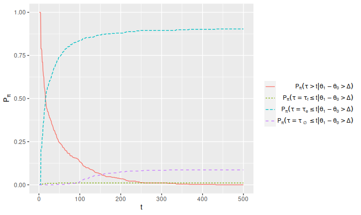
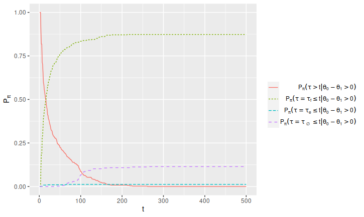
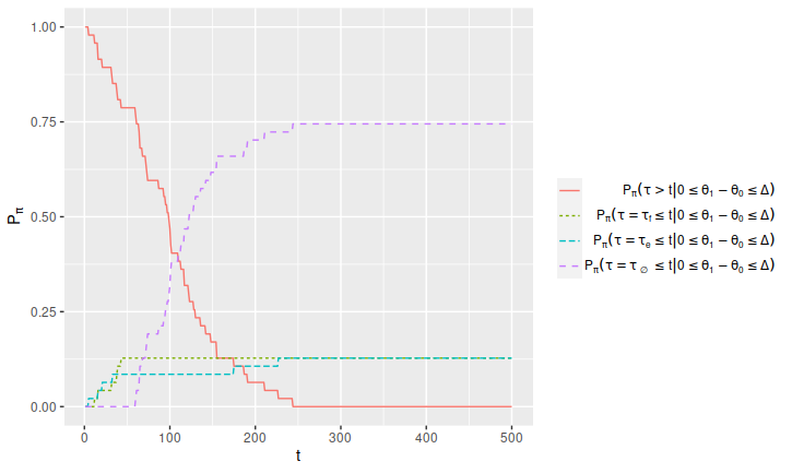
Figure 1: Predictive probabilities for different ways of stopping a trial by the time the outcomes from $t$ patients have been observed, subdivided according to the conclusion made (efficacy, futility, or inconclusive). Monte Carlo samples of size 1000 were used in each step for evaluating the considered posterior probabilities and the predictive expected utilities.

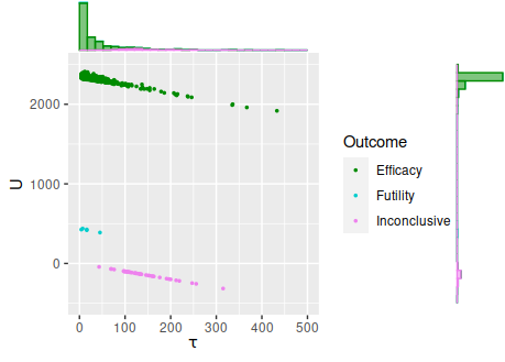
((a)) $\mathbb{E}_{\pi}\bigl{(}U_{\tau}\big{|}\bftheta_{1}-\bftheta_{0}>\Delta\bigr{)}=2089.62$

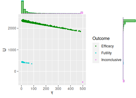
((b)) $\mathbb{E}_{\pi}\bigl{(}U_{\tau}\big{|}\bftheta_{1}-\bftheta_{0}>\Delta\bigr{)}=2093.77$

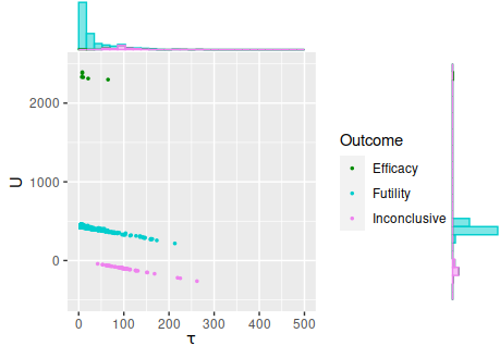
((c)) $\mathbb{E}_{\pi}\bigl{(}U_{\tau}\big{|}\bftheta_{1}-\bftheta_{0}<0\bigr{)}=377.70$

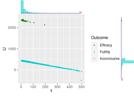
((d)) $\mathbb{E}_{\pi}\bigl{(}U_{\tau}\big{|}\bftheta_{1}-\bftheta_{0}<0\bigr{)}=382.19$

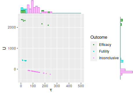
((e)) $\mathbb{E}_{\pi}\bigl{(}U_{\tau}\big{|}0\leq\bftheta_{1}-\bftheta_{0}\leq\Delta\bigr{)}=257.66$

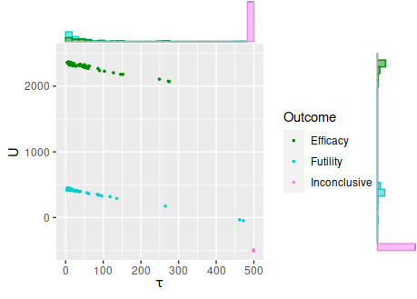
((f)) $\mathbb{E}_{\pi}\bigl{(}U_{\tau}\big{|}0\leq\bftheta_{1}-\bftheta_{0}\leq\Delta\bigr{)}=196.76$

Figure 2: An illustration of the effect of including the ’early stopping’ -option in the design (for an explanation, see text). Scatter plots and marginal histograms based on simulated samples from the conditional joint distribution of $\tau$ and the corresponding conditional expectation of final utility, under $\mathbb{P}_{\pi}$ and given the respective efficacy $\{\bftheta_{1}-\bftheta_{0}>\Delta\}$, futility $\{\bftheta_{1}-\bftheta_{0}<0\}$ and inconclusive $\{0\leq\bftheta_{1}-\bftheta_{0}\leq\Delta\}$ alternatives. The expectations in each case are computed as sample averages. The simulation parameters are the same as for Figure 1.

5 Discussion

Clinical trials are an instrument for making informed decisions based on experimental data. In phase II trials, the usual goal is to make a comparative evaluation on the efficacy of an experimental treatment to a control, and in multi-arm trials, also to each other. More successful treatments among the considered alternatives, if found, can then be selected for further study, possibly in phase III. While the presentation here is based on considering phase II, essentially the same ideas and methods could be used also in phase III, and even in a seamless fashion by only making an appropriate adjustment to the values of the design parameters.

Such conclusions should be made using relevant prior information and the data coming from the trial itself, with the prior being based on trusted expert assessments and, whenever possible, on existing empirical data from comparable treatments. This is precisely what the consequent Bayesian posterior distributions synthesize and express. Compelling arguments justifying their use in the context of clinical trials have been presented in the literature since [5] and [43]. For a recent commentary, see the blog of [22]. Importantly, [22] contains a demonstration of how decisions based on stopping boundaries for Bayesian posteriors are well calibrated.

In this paper, in the case of a 2-arm superiority trial, we considered posterior probabilities of the form $\mathbb{P}_{\pi}(\bftheta_{1}-\bftheta_{0}\leq\Delta|{\mathcal{D}}_{n})$. Efficacy of the experimental treatment would then be concluded if this probability falls below the selected threshold $\varepsilon_{e}$, the maximal posterior risk allowed for that such a conclusion would be wrong, thereby representing a selected risk tolerance. A similar criterion, based on posterior probabilities $\mathbb{P}_{\pi}(\bftheta_{1}-\bftheta_{0}\geq 0|{\mathcal{D}}_{n})$, was provided for concluding futility. The decision rule was further complemented to a form that allows the trial to be stopped early if the predicted chances of arriving at either of these definitive final conclusions are thin.

The rule for early stopping is an adaptation and generalization of the stage-wise method of [7]. The idea is to consider, in interim analyses carried out progressively over time, the expected future gains and losses, evaluated with respect to the current posterior predictive distribution, in the event that the trial were to be continued. If such future expectations are negative, the trial is stopped even though neither efficacy nor futility has been concluded.

The decision rules considered here for superiority trials are easily modified to be appropriate for equivalence and non-inferiority trials as well. For example, for the latter, we would be led to considering posterior probabilities of the form $\mathbb{P}_{\pi}(\bftheta_{1}-\bftheta_{0}\geq-\Delta|{\mathcal{D}}_{n})$, where $\Delta$ is a selected non-inferiority margin. Moreover, the prototype case of binary outcomes measured soon after treatment can be modified to other types of outcome data, without changing the logical basis of the method, as long as the relevant posterior probabilities are computable from the accruing data. Extensions into multi-arm designs, and thereby applying adaptive rules for treatment assignment, seem also feasible ([1]).

We have for simplicity considered the case where the posterior probabilities are updated systematically after a new outcome has been measured. This need not be so, and less frequent stage-wise interim checks will generally lead to lower logistic and computational costs. On the other hand, such thinning of the data sequence has the effect that some of the conclusions that would have been otherwise made are then postponed to a later time, or even go unnoticed.

A central issue in this paper has been our attempt to find a satisfactory answer to the question: If the statistical analysis of trial data is done by applying the tools from Bayesian inference and decision theory, how should one react to the regulators’ common requirement to control the Type 1 error rate as a method to guard against false positives?

We have been critical towards applying the Frequentist-oriented Perspective, as described by [51], for reasons that are both conceptual and practical. It is a hybrid approach which both relies on the likelihood principle and violates it. For computing the value of Type 1 error rate in a design one needs to account in advance for all possible ways of making errors in concluding efficacy that may turn up when the trial is to be run. Full compliance with this requirement seriously limits the possibilities of introducing and employing more flexible adaptive trial designs. Systematic sequential monitoring of the outcomes from the trial, and making corresponding interim checks, may be avoided in practice for valid reasons such as greater complexity in the required logistics, more elaborate computations, or because it is argued that the consequent unblinding could jeopardize the whole study. However, looking from a Bayesian perspective, avoiding interim checks because this would inflate the Type 1 error rate is an unnecessary artefact due to not respecting the conditionality principle. Additional insightful comments on the implications of applying the likelihood principle in the clinical trials context can be found in [23].

In their outline of the Calibrated Bayesian Perspective, [51] suggest employment of two probability distributions as descriptions of the treatment effects, a "subjective" Bayesian prior specified by the investigators and used in the analysis of the trial data, and another, equipped with a frequentist interpretation, to represent the background information of the regulators. [51] then proposed that a new criterion called FDR, interpreted as the relative proportion of false claims among all claims of efficacy "in the infinite series of trials for a range of plausible" combinations of treatment effects and trial outcomes, could replace the standard control of Type 1 error rate. According to [51], "Metrics like the FDR … have not been used for drug approval, but arguably, they reflect the reality better than frequentist properties." We agree.

The proposed FDR criterion has the mathematical form of a conditional probability. More exactly, if the distribution representing the regulators’ assessments in the above "infinite series of trials" is understood as the prior and a concluded efficacy result from the trial as the conditioning event, it is the posterior probability of that this conclusion is false. This probability is likely to be immediately meaningful to both the regulators and the investigators, and therefore discussing its value at the time a trial is designed, and bounding such a value numerically, should be an attractive option for both parties.

However, it is problematic if the regulators and the investigators impose mutually inconsistent means for the error control of the trial. The problem is solved if they agree on a common distribution that would represent a shared understanding on the likely size of the treatment effects. It makes no harm if the regulators prefer a frequentist "infinite series" interpretation for this distribution, whereas the investigators, having in the design suggested use of Bayesian methods in the analysis of the trial data, will be naturally inclined to applying an epistemic interpretation. The consequent cFDR criterion is then for both parties a valid quantification of the possibility, if the trial ends by concluding efficacy, of that this is false. A bonus from the agreement is that the error tolerance against such conclusions during the data analysis is automatically also an upper bound for cFDR.

Currently the regulators receive only rarely requests to handle Bayesian trial designs for possible approval. This may, in part, be a consequence of the general perception among the investigators with Bayesian leanings that the approval of such designs would be difficult. Methodological conservatism, combined with lacking familiarity with the Bayesian principles, and even prejudices towards such methods based on superficially understood notions of "subjective" and "objective" in science (cf. [12]), are not uncommon on either side of the table. In this situation one would wish that both parties would engage themselves actively in an open discussion, without preconceived fixes of right and wrong. The issues are important and the potential benefits from methodological progress based on conceptually clear and scientifically sound arguments are large. But it takes two to tango…

Appendix A Notes on the analytic and numerical computation of some double Beta integrals

Lemma A.1.

1. A random variable $\bftheta$ is $\mbox{Beta}(\alpha,\beta)$-distributed if and only if $(1-\bftheta)$ is $\mbox{Beta}(\beta,\alpha)$-distributed

2. The incomplete Beta function has representation

   $$\int_{0}^{x}y^{\alpha-1}(1-y)^{\beta-1}dy=\frac{x^{\alpha}}{\alpha}{}_{2}F_{1}\bigl{(}\alpha,1-\beta;\alpha+1;x\bigr{)}=\frac{x^{\alpha}(1-x)^{\beta}}{\alpha}{}_{2}F_{1}\bigl{(}\alpha+\beta,1;\alpha+1;x\bigr{)}$$

   $$=\int_{1-x}^{1}(1-y)^{\alpha-1}y^{\beta-1}dy=\frac{\Gamma(\alpha)\Gamma(\beta)}{\Gamma(\alpha+\beta)}-\frac{(1-x)^{\beta}}{\beta}{}_{2}F_{1}\bigl{(}\beta,1-\alpha,\beta+1,1-x\bigr{)}$$

   where ${}_{2}F_{1}(a,b;c;x)$ is the Gauss hypergeometric function.

3. Gauss generalized hypergeometric function satisfies

   $$\frac{\Gamma(\alpha+\beta)}{\Gamma(\alpha)\Gamma(\beta)}\int_{0}^{1}x^{\alpha-1}(1-x)^{\beta-1}{}_{p}F_{q}(a_{1},\dots,a_{p};b_{1},\dots,b_{q};xy)dx$$

   $$={}_{p+1}F_{q+1}(a_{1},\dots,a_{p},\alpha;b_{1},\dots,b_{q},\alpha+\beta;y)$$

4. $$\int_{0}^{1}x^{\gamma-1}(1-x)^{\rho-1}(1-zx)^{-\sigma}{}_{2}F_{1}\bigl{(}\alpha,\beta;\gamma;x\bigr{)}dx$$

   $$=(1-z)^{\sigma}\frac{\Gamma(\gamma)\Gamma(\rho)\Gamma(\gamma+\rho-\alpha-\beta)}{\Gamma(\gamma+\rho-\alpha)\Gamma(\gamma+\rho-\beta)}{}_{3}F_{2}\bigl{(}\rho,\sigma,\gamma+\rho-\alpha-\beta;\gamma+\rho-\alpha,\gamma+\rho-\beta;\frac{z}{z-1}\bigr{)}$$

   for $\Re(\gamma),\Re(\rho),\Re(\gamma+\rho-\alpha-\beta)>0,|\arg(1-x)|<\pi$ (7.512.9 in [21]).

5. $$(1-x)^{\alpha}={}_{1}F_{0}(\alpha;x)={}_{2}F_{1}(\alpha,\beta;\beta;x)$$

Lemma A.2.

1. $$\mathbb{P}\bigl{(}\bftheta_{1}<\bftheta_{0})=\frac{\Gamma(\alpha_{0}+\beta_{0})\Gamma(\alpha_{1}+\beta_{1})}{\Gamma(\alpha_{0})\Gamma(\beta_{0})\Gamma(\alpha_{1})\Gamma(\beta_{1})}\int_{0}^{1}\int_{0}^{x}y^{\alpha_{1}-1}(1-y)^{\beta_{1}-1}dy\;x^{\alpha_{0}-1}(1-x)^{\beta_{0}-1}dx=$$

   $$\frac{\Gamma(\alpha_{0}+\alpha_{1})\Gamma(\beta_{0}+\beta_{1})\Gamma(\alpha_{0}+\beta_{0})\Gamma(\alpha_{1}+\beta_{1})}{\Gamma(\alpha_{0}+\alpha_{1}+\beta_{0}+\beta_{1})\Gamma(\alpha_{0})\Gamma(\beta_{0})\Gamma(\alpha_{1}+1)\Gamma(\beta_{1})}\times$$

   $${}_{3}F_{2}(\alpha_{1}+\beta_{1},1,\alpha_{0}+\alpha_{1};\alpha_{1}+1,\alpha_{0}+\alpha_{1}+\beta_{0}+\beta_{1};1)$$

   where the ${}_{3}F_{2}(a_{1},a_{2},a_{3};b_{1},b_{2};z)$ hypergeometric function is convergent for $|z|<1$, and also when $|z|=1$ and $\Re\biggl{(}\sum_{k=1}^{2}b_{k}-\sum_{j=1}^{3}a_{j}\biggr{)}>0$

2. We have also

   $$\mathbb{P}(\bftheta_{1}<c\bftheta_{0})=\frac{\Gamma(\alpha_{0}+\beta_{0})\Gamma(\alpha_{1}+\beta_{1})}{\Gamma(\alpha_{0})\Gamma(\beta_{0})\Gamma(\alpha_{1})\Gamma(\beta_{1})}\int_{0}^{1}\int_{0}^{x/c}y^{\alpha_{1}-1}(1-y)^{\beta_{1}-1}dy\;x^{\alpha_{0}-1}(1-x)^{\beta_{0}-1}dx=$$

   $$\frac{\Gamma(\alpha_{0}+\beta_{0})\Gamma(\alpha_{1}+\beta_{1})c^{\alpha_{0}}}{\Gamma(\alpha_{0})\Gamma(\beta_{0})\Gamma(\alpha_{1})\Gamma(\beta_{1})}\int_{0}^{1}\int_{0}^{u}y^{\alpha_{1}-1}(1-y)^{\beta_{1}-1}dy\;u^{\alpha_{0}-1}(1-cu)^{\beta_{0}-1}du=$$

   $$\frac{\Gamma(\alpha_{0}+\beta_{0}-1)\Gamma(\alpha_{0}+\alpha_{1})\Gamma(\alpha_{0}+\beta_{0})\Gamma(\alpha_{1}+\beta_{1})c^{\alpha_{0}}(1-c)^{1-\beta_{0}}}{\Gamma(\alpha_{0}+\alpha_{1}+\beta_{0}-1)\Gamma(\alpha_{0})^{2}\Gamma(\beta_{0})\Gamma(\alpha_{1})\Gamma(\beta_{1})}\times$$

   $${}_{3}F_{2}\biggl{(}0,1-\beta_{0},\alpha_{0}+\beta_{1}-1;\alpha_{0}+\alpha_{1}+\beta_{1}-1;\frac{c}{c-1}\biggr{)}$$

3. $$\mathbb{P}(\bftheta_{1}<\bftheta_{0}+\Delta)=$$

   $$\frac{\Gamma(\alpha_{0}+\beta_{0})\Gamma(\alpha_{1}+\beta_{1})}{\Gamma(\alpha_{0})\Gamma(\beta_{0})\Gamma(\alpha_{1})\Gamma(\beta_{1})}\int_{0}^{1}\int_{0}^{1\wedge(x+\Delta)}y^{\alpha_{1}-1}(1-y)^{\beta_{1}-1}dy\;x^{\alpha_{0}-1}(1-x)^{\beta_{0}-1}dx$$

   For $\Delta>0$

   $$=\frac{\Gamma(\alpha_{0}+\beta_{0})\Gamma(\alpha_{1}+\beta_{1})\Delta^{\alpha_{1}}}{\Gamma(\alpha_{0})\Gamma(\beta_{0})\Gamma(\alpha_{1})\Gamma(\beta_{1})\alpha_{1}}\int_{0}^{1-\Delta}\bigl{(}1+\frac{x}{\Delta}\bigr{)}^{\alpha_{1}}{}_{2}F_{1}\bigl{(}\alpha_{1},1-\beta_{1};\alpha_{1}+1;x+\Delta\bigr{)}x^{\alpha_{0}-1}(1-x)^{\beta_{0}-1}dx$$

   $$+\frac{\Gamma(\alpha_{0}+\beta_{0})}{\Gamma(\alpha_{0})\Gamma(\beta_{0})}\int_{1-\Delta}^{1}x^{\alpha_{0}-1}(1-x)^{\beta_{0}-1}dx=$$

   $$\frac{\Gamma(\alpha_{0}+\beta_{0})\Gamma(\alpha_{1}+\beta_{1})\Delta^{\alpha_{1}}}{\Gamma(\alpha_{0})\Gamma(\beta_{0})\Gamma(\alpha_{1})\Gamma(\beta_{1})\alpha_{1}}\int_{0}^{1-\Delta}{}_{1}F_{0}\bigl{(}\alpha_{1};-\frac{x}{\Delta}\bigr{)}{}_{2}F_{1}\bigl{(}\alpha_{1},1-\beta_{1};\alpha_{1}+1;x+\Delta\bigr{)}x^{\alpha_{0}-1}(1-x)^{\beta_{0}-1}dx$$

   $$+\frac{\Gamma(\alpha_{0}+\beta_{0})}{\Gamma(\alpha_{0})\Gamma(\beta_{0})}\frac{\Delta^{\beta_{0}}}{\beta_{0}}{}_{2}F_{1}(\beta_{0},1-\alpha_{0};\beta_{0}+1;\Delta)$$

A.1 Innovation Gain formulae updating the posterior in Bayesian Filtering

For $\bftheta\sim\mbox{Beta}(\alpha,\beta)$, by using integration by parts we obtain the following Stein equation for the Beta distribution

$$\frac{\alpha\beta}{(\alpha+\beta)(\alpha+\beta+1)}\mathbb{E}_{\alpha+1,\beta+1}\bigl{[}\partial f(\bftheta)\bigr{]}=\mathbb{E}_{\alpha,\beta}\bigl{[}\bftheta(1-\bftheta)\partial f(\bftheta)\bigr{)}=$$

$$\mathbb{E}_{\alpha,\beta}\bigl{[}\bigl{(}(\beta+\alpha)\bftheta-\alpha\bigr{)}f(\bftheta)\bigr{]}=\alpha\bigl{\{}\mathbb{E}_{\alpha+1,\beta}\bigl{[}f(\bftheta)\bigr{]}-\mathbb{E}_{\alpha,\beta}\bigl{[}f(\bftheta)\bigr{]}\bigr{\}}$$

For $f(\theta)={\bf 1}(\theta>t)$, $\partial f(\theta)=\Delta_{t}(\theta)$, the Dirac delta function, which gives

$$\mathbb{P}_{\alpha+1,\beta}(\bftheta>t)=\mathbb{P}_{\alpha,\beta}(\bftheta>t)+\frac{\Gamma(\alpha+\beta)}{\Gamma(\alpha+1)\Gamma(\beta)}t^{\alpha}(1-t)^{\beta}$$

$$=\mathbb{P}_{\alpha,\beta}(\bftheta>t)+\alpha^{-1}\mbox{Beta}(\alpha,\beta)^{-1}t^{\alpha}(1-t)^{\beta}$$

which can be used to update the posterior recursively. We have also

$$\mathbb{P}_{\alpha+1,\beta}(\bftheta\leq t)-\mathbb{P}_{\alpha,\beta}(\bftheta\leq t)=-\alpha^{-1}\mbox{Beta}(\alpha,\beta)^{-1}t^{\alpha}(1-t)^{\beta}$$

and

$$\mathbb{P}_{\alpha,\beta+1}(\bftheta\leq t)=\mathbb{P}_{\alpha,\beta+1}(1-\bftheta\geq 1-t)=\mathbb{P}_{\beta+1,\alpha}(\bftheta\geq 1-t)=$$

$$\mathbb{P}_{\alpha,\beta}(\bftheta\leq t)+\beta^{-1}\mbox{Beta}(\alpha,\beta)^{-1}t^{\alpha}(1-t)^{\beta}$$

By integrating we obtain for $\bftheta_{0},\bftheta_{1}$ with independent Beta$(\alpha_{i},\beta_{i})$ priors

$$\bigl{(}\mathbb{P}_{\alpha_{0}+1,\beta_{0}}\otimes\mathbb{P}_{\alpha_{1},\beta_{1}}\bigr{)}\bigl{(}\bftheta_{0}>\bftheta_{1}\bigr{)}-\bigl{(}\mathbb{P}_{\alpha_{0},\beta_{0}}\otimes\mathbb{P}_{\alpha_{1},\beta_{1}}\bigr{)}\bigl{(}\bftheta_{0}>\bftheta_{1}\bigr{)}=$$

$$\frac{\Gamma(\alpha_{0}+\beta_{0})}{\Gamma(\alpha_{0}+1)\Gamma(\beta_{0})}\frac{\Gamma(\alpha_{1}+\beta_{1})}{\Gamma(\alpha_{1})\Gamma(\beta_{1})}\frac{\Gamma(\alpha_{0}+\alpha_{1})\Gamma(\beta_{0}+\beta_{1})}{\Gamma(\alpha_{0}+\alpha_{1}+\beta_{0}+\beta_{1})}$$

$$=\frac{\mbox{Beta}(\alpha_{0}+\alpha_{1},\beta_{0}+\beta_{1})}{\alpha_{0}\mbox{Beta}(\alpha_{0},\beta_{0})\mbox{Beta}(\alpha_{1},\beta_{1})}$$

and

$$\bigl{(}\mathbb{P}_{\alpha_{0},\beta_{0}+1}\otimes\mathbb{P}_{\alpha_{1},\beta_{1}}\bigr{)}\bigl{(}\bftheta_{0}\leq\bftheta_{1}\bigr{)}-\bigl{(}\mathbb{P}_{\alpha_{0},\beta_{0}}\otimes\mathbb{P}_{\alpha_{1},\beta_{1}}\bigr{)}\bigl{(}\bftheta_{0}\leq\bftheta_{1}\bigr{)}$$

$$=\frac{\mbox{Beta}(\beta_{0}+\beta_{1},\alpha_{0}+\alpha_{1})}{\beta_{0}\mbox{Beta}(\beta_{0},\alpha_{0})\mbox{Beta}(\beta_{1},\alpha_{1})}$$

see [49]. We derive also expressions for the innovation gain in the Bayes filtering formula sequentially updating the posterior distribution

$$\bigl{(}\mathbb{P}_{\alpha_{0}+1,\beta_{0}}\otimes\mathbb{P}_{\alpha_{1},\beta_{1}}\bigr{)}\bigl{(}\bftheta_{0}>\bftheta_{1}+{\Delta}\bigr{)}-\bigl{(}\mathbb{P}_{\alpha_{0},\beta_{0}}\otimes\mathbb{P}_{\alpha_{1},\beta_{1}}\bigr{)}\bigl{(}\bftheta_{0}>\bftheta_{1}+{\Delta}\bigr{)}=$$

$$\alpha_{0}^{-1}\mbox{Beta}(\alpha_{0},\beta_{0})^{-1}\mbox{Beta}(\alpha_{1},\beta_{1})^{-1}\int_{{\Delta}^{-}}^{1-{\Delta}^{+}}t^{\alpha_{1}-1}(1-t)^{\beta_{1}-1}(t+{\Delta})^{\alpha_{0}}(1-{\Delta}-t)^{\beta_{0}}dt$$

$$=\alpha_{0}^{-1}\mbox{Beta}(\alpha_{0},\beta_{0})^{-1}\mathbb{E}_{\alpha_{1},\beta_{1}}\biggl{(}\bigl{\{}(\bftheta_{1}+{\Delta})^{+}\bigr{\}}^{\alpha_{0}}\bigl{\{}(1-\bftheta_{1}-{\Delta})^{+}\bigr{\}}^{\beta_{0}}\biggr{)}=$$

$$\frac{\beta_{0}}{(\alpha_{0}+\beta_{0})(\alpha_{0}+\beta_{0}+1)\mbox{Beta}(\alpha_{1},\beta_{1})}\mathbb{E}_{\alpha_{0}+1,\beta_{0}+1}\biggl{(}\bigl{\{}(\bftheta_{0}-{\Delta})^{+}\bigr{\}}^{\alpha_{1}-1}\bigl{\{}(1+{\Delta}-\bftheta_{0})^{+}\bigr{\}}^{\beta_{1}-1}\biggr{)}=$$

$$\alpha_{0}^{-1}\mbox{Beta}(\alpha_{0},\beta_{0})^{-1}\mbox{Beta}(\alpha_{1},\beta_{1})^{-1}\times$$

$$\sum_{k=0}^{\infty}\sum_{\ell=0}^{k}{\Delta}^{k}(-1)^{\ell}\frac{(\beta_{0})_{\ell}(\alpha_{0})_{k-\ell}}{\ell!(k-\ell)!}\int_{{\Delta}^{-}}^{1-{\Delta}^{+}}(1-t)^{\beta_{0}+\beta_{1}-\ell-1}t^{\alpha_{0}+\alpha_{1}+\ell-k-1}dt$$

$$=\alpha_{0}^{-1}\mbox{Beta}(\alpha_{0},\beta_{0})^{-1}\mbox{Beta}(\alpha_{1},\beta_{1})^{-1}\times$$

$$\sum_{k=0}^{\infty}\sum_{\ell=0}^{k}{\Delta}^{k}(-1)^{\ell}\frac{(\beta_{0})_{\ell}(\alpha_{0})_{k-\ell}}{\ell!(k-\ell)!(\alpha_{0}+\alpha_{1}+\ell-k)}\times$$

$$\biggl{\{}(1-{\Delta}^{+})^{\alpha_{0}+\alpha_{1}+\ell-k}{}_{2}F_{1}(\alpha_{0}+\alpha_{1}+\ell-k,1+\ell-\beta_{0}-\beta_{1};1+\alpha_{0}+\alpha_{1}+\ell-k;1-{\Delta}^{+})$$

$$-({\Delta}^{-})^{\alpha_{0}+\alpha_{1}+\ell-k}{}_{2}F_{1}(\alpha_{0}+\alpha_{1}+\ell-k,1+\ell-\beta_{0}-\beta_{1};1+\alpha_{0}+\alpha_{1}+\ell-k;{\Delta}^{-})\biggr{\}}$$

with ${\Delta}^{+}=\max\{{\Delta},0\}$ ${\Delta}^{-}=\max\{-{\Delta},0\}$, and we have used the generalized Newton binomial formula where $(\alpha)_{k}=\alpha(\alpha-1)\dots(\alpha-k+1)$ is the Pochammer symbol. We have also the updates

$$\bigl{(}\mathbb{P}_{\alpha_{0}+1,\beta_{0}}\otimes\mathbb{P}_{\alpha_{1},\beta_{1}}\bigr{)}\bigl{(}\bftheta_{0}+{\Delta}<\bftheta_{1}\bigr{)}-\bigl{(}\mathbb{P}_{\alpha_{0},\beta_{0}}\otimes\mathbb{P}_{\alpha_{1},\beta_{1}}\bigr{)}\bigl{(}\bftheta_{0}+{\Delta}<\bftheta_{1}\bigr{)}=$$

$$=-\alpha_{0}^{-1}\mbox{Beta}(\alpha_{0},\beta_{0})^{-1}\mathbb{E}_{\alpha_{1},\beta_{1}}\biggl{(}\bigl{\{}(\bftheta_{1}-{\Delta})^{+}\bigr{\}}^{\alpha_{0}}\bigl{\{}(1-\bftheta_{1}+{\Delta})^{+}\bigr{\}}^{\beta_{0}}\biggr{)}$$

$$\bigl{(}\mathbb{P}_{\alpha_{0},\beta_{0}+1}\otimes\mathbb{P}_{\alpha_{1},\beta_{1}}\bigr{)}\bigl{(}\bftheta_{0}>\bftheta_{1}+{\Delta}\bigr{)}-\bigl{(}\mathbb{P}_{\alpha_{0},\beta_{0}}\otimes\mathbb{P}_{\alpha_{1},\beta_{1}}\bigr{)}\bigl{(}\bftheta_{0}>\bftheta_{1}+{\Delta}\bigr{)}=$$

$$\bigl{(}\mathbb{P}_{\beta_{0}+1,\alpha_{0}}\otimes\mathbb{P}_{\beta_{1},\alpha_{1}}\bigr{)}\bigl{(}\bftheta_{1}>\bftheta_{0}+{\Delta}\bigr{)}-\bigl{(}\mathbb{P}_{\beta_{0},\alpha_{0}}\otimes\mathbb{P}_{\beta_{1},\alpha_{1}}\bigr{)}\bigl{(}\bftheta_{1}>\bftheta_{0}+{\Delta}\bigr{)}=$$

$$-\beta_{0}^{-1}\mbox{Beta}(\beta_{0},\alpha_{0})^{-1}\mathbb{E}_{\beta_{1},\alpha_{1}}\biggl{(}\bigl{\{}(\bftheta_{1}-{\Delta})^{+}\bigr{\}}^{\beta_{0}}\bigl{\{}(1-\bftheta_{1}+{\Delta})^{+}\bigr{\}}^{\alpha_{0}}\biggr{)}$$

$$\bigl{(}\mathbb{P}_{\alpha_{0},\beta_{0}+1}\otimes\mathbb{P}_{\alpha_{1},\beta_{1}}\bigr{)}\bigl{(}\bftheta_{0}+{\Delta}<\bftheta_{1}\bigr{)}-\bigl{(}\mathbb{P}_{\alpha_{0},\beta_{0}}\otimes\mathbb{P}_{\alpha_{1},\beta_{1}}\bigr{)}\bigl{(}\bftheta_{0}+{\Delta}<\bftheta_{1}\bigr{)}$$

$$=\beta_{0}^{-1}\mbox{Beta}(\beta_{0},\alpha_{0})^{-1}\mathbb{E}_{\beta_{1},\alpha_{1}}\biggl{(}\bigl{\{}(\bftheta_{1}+{\Delta})^{+}\bigr{\}}^{\beta_{0}}\bigl{\{}(1-\bftheta_{1}-{\Delta})^{+}\bigr{\}}^{\alpha_{0}}\biggr{)}$$

When $\alpha_{j},\beta_{j}\in\mathbb{N}$, $\forall j=0,1\dots,K$, the innovation gain in the filtering formula for $\mathbb{P}(\bftheta_{0}+\Delta<\bftheta_{1}|{\mathcal{D}}_{t})$ has analytic expression.

A.2 Efficient Monte Carlo approximation

The computation of Beta functions and hypergeometric functions appearing in the innovation formulae for large values of the beta distributions parameters is prone to severe numerical instability. A simple and robust numerical alternative is to the evaluate the posterior probabilities $\mathbb{P}(\bftheta_{0}>\bftheta_{1}|{\mathcal{D}}_{t})$ and $\mathbb{P}(\bftheta_{1}>\bftheta_{0}+\Delta|{\mathcal{D}}_{t})$ by using plain Monte Carlo in the most efficient way. Let $X,Y$ be independent random variables with respective cumulative distribution functions $F,G$. An estimator of

$$\mathbb{P}(X>Y)=\int_{\mathbb{R}}\int_{\mathbb{R}}{\bf 1}(x>y)F(dx)G(dy),$$

based on independent realizations $(X_{k},Y_{k}:k=1,\dots,n),$ is given by

$$\widehat{\mathbb{P}}_{n}(X>Y)=\int_{\mathbb{R}}\int_{\mathbb{R}}{\bf 1}(x>y)F_{n}(dx)G_{n}(dy)=\frac{1}{n^{2}}\sum_{j=1}^{n}\sum_{k=1}^{n}{\bf 1}(X_{j}>Y_{k}),$$

where $F_{n},G_{n}$ are the respective empirical processes. Asymptotically $\sqrt{n}(F_{n}(x)-F(x))\longrightarrow B(x)$ and $\sqrt{n}(G_{n}(y)-G(y))\longrightarrow Z(y)$, which are zero mean Brownian bridge processes $B(x),Z(y)$ with respective covariances $\mathbb{E}(B(x)B(x^{^{\prime}})=F(x\wedge x^{^{\prime}})-F(x)F(x^{^{\prime}})$ and $\mathbb{E}(Z(y)Z(y^{^{\prime}}))=G(y\wedge y^{^{\prime}})-G(y)G(y^{^{\prime}})$. The estimator $\widehat{\mathbb{P}}_{n}(X>Y)$ is unbiased and, by the functional delta method,

$$\sqrt{n}\bigl{(}\widehat{\mathbb{P}}_{n}(X>Y))-\mathbb{P}(X>Y)\bigr{)}$$

is asymptotically zero mean Gaussian with variance

$$\sigma^{2}=\int_{\mathbb{R}}(1-F(y))^{2}G(dy)-\biggl{(}\int_{\mathbb{R}}(1-F(y))G(dy)\biggr{)}^{2}+\int_{\mathbb{R}}G(x)^{2}F(dx)-\biggl{(}\int_{\mathbb{R}}G(x)F(dx)\biggr{)}^{2}$$

$$=\text{Var}_{G}\bigl{(}F(Y)\bigr{)}+\text{Var}_{F}\bigl{(}G(X)\bigr{)}.$$

Computing $\widehat{P}_{n}$ requires $n$ independent samples from both distributions $F,G$, sorting the combined samples and doing on average $2n\log(2n)$ comparisons, achieving asymptotic standard deviation $\sigma n^{-1/2}$. The naive estimator based on the same samples

$$\check{\mathbb{P}}_{n}(X>Y)=\frac{1}{n}\sum_{k=1}^{n}{\bf 1}(X_{k}>Y_{k}),$$

requiring $n$ comparisons, is also unbiased and

$$\sqrt{n}\bigl{(}\check{\mathbb{P}}_{n}(X>Y)-\mathbb{P}(X>Y)\bigr{)}$$

is asymptotically Gaussian with zero mean and variance

$$\eta^{2}=\mathbb{P}\bigl{(}X>Y)-\mathbb{P}\bigl{(}X>Y)^{2}=\mathbb{E}_{F}(G(X))-\mathbb{E}_{F}(G(X))^{2}=\mathbb{E}_{G}(1-F(Y))-\mathbb{E}_{G}(1-F(Y))^{2}.$$

For $X,X^{^{\prime}},Y,Y^{^{\prime}}$ independent random variables with $X,X^{^{\prime}}\sim F$ and $Y,Y^{^{\prime}}\sim G$,

$$\eta^{2}-\sigma^{2}=\frac{1}{4}\mathbb{E}\biggl{[}\biggl{(}{\bf 1}(X>Y)-{\bf 1}(X>Y^{^{\prime}})+{\bf 1}(X^{^{\prime}}>Y^{^{\prime}})-{\bf 1}(X^{^{\prime}}>Y)\biggr{)}^{2}\biggr{]}\geq 0.$$

In practice the computational cost of comparing variables is much smaller than the cost of sampling random variables, and it is computationally more efficient to make $2n\log(2n)>n$ comparisons in order to achieve the smaller constant $\sigma^{2}\leq\eta^{2}$ in the asymptotic error variance (see also [26]).

References

- [1] Elja Arjas and Dario Gasbarra “Adaptive treatment allocation and selection in multi-arm clinical trials: a Bayesian perspective” In BMC Med Res Methodol 22.1 Springer ScienceBusiness Media LLC, 2022 DOI: 10.1186/s12874-022-01526-8
- [2] Andrea Bassi, Johannes Berkhof, Daphne Jong and Peter M Ven “Bayesian adaptive decision-theoretic designs for multi-arm multi-stage clinical trials” In Stat Methods Med Res 30.3 SAGE Publications Sage UK: London, England, 2021, pp. 717–730
- [3] Jonathan Beall, Christy N Cassarly and Renee L Martin “Interpreting a Bayesian phase II futility clinical trial” In Trials 23, 2022
- [4] Yoav Benjamini and Yosef Hochberg “Controlling the False Discovery Rate: A Practical and Powerful Approach to Multiple Testing” In J R Stat Soc Series B Stat Methodol 57.1, 1995, pp. 289–300 DOI: https://doi.org/10.1111/j.2517-6161.1995.tb02031.x
- [5] Donald A. Berry “Interim analyses in clinical trials: classical vs. Bayesian approaches” In Stat Med 4.4 Wiley Online Library, 1985, pp. 521–526
- [6] Bradley P Carlin, Joseph B Kadane and Alan E Gelfand “Approaches for optimal sequential decision analysis in clinical trials” In Biometrics JSTOR, 1998, pp. 964–975
- [7] Yi Cheng and Yu Shen “Bayesian adaptive designs for clinical trials” In Biometrika 92.3 Oxford University Press, 2005, pp. 633–646
- [8] Sylvie Chevret “Bayesian adaptive clinical trials: a dream for statisticians only?” In Stat Med 31.11-12 Wiley Online Library, 2012, pp. 1002–1013
- [9] Nigel Dallow and Paolo Fina “The perils with the misuse of predictive power” In Pharm Stat 10.4 Wiley Online Library, 2011, pp. 311–317
- [10] A.. Dawid “The Well-Calibrated Bayesian” In J Am Stat Assoc 77.379 Taylor & Francis, 1982, pp. 605–610 DOI: 10.1080/01621459.1982.10477856
- [11] Alexei Dmitrienko and Ming-Dauh Wang “Bayesian predictive approach to interim monitoring in clinical trials” In Stat Med 25.13 Wiley Online Library, 2006, pp. 2178–2195
- [12] David Draper “Coherence and calibration: comments on subjectivity and "objectivity" in Bayesian analysis (comment on articles by Berger and by Goldstein)” In Bayesian Anal 1.3, 2006, pp. 423–428
- [13] David Draper and Milovan Krnjajic “Calibration results for Bayesian model specification” In Bayesian Anal 1.1, 2010, pp. 1–43
- [14] Food and Drug Administration “Guidance for the Use of Bayesian Statistics in Medical Device Clinical Trials.”, 2010
- [15] Food and Drug Administration “Adaptive Designs for Clinical Trials of Drugs and Biologics: Guidance for Industry.”, 2019
- [16] Benjamin Freedman “Equipoise and the ethics of clinical research” In N Engl J Med 317.3 Massachusetts Medical Society, 1987, pp. 141–145
- [17] Laurence S Freedman, David J Spiegelhalter and Mahesh KB Parmar “The what, why and how of Bayesian clinical trials monitoring” In Stat Med 13.13-14 Wiley Online Library, 1994, pp. 1371–1383
- [18] Seymour Geisser and Wesley Johnson “Interim analysis for normally distributed observables” In Lect Notes Monogr Ser JSTOR, 1994, pp. 263–279
- [19] Christian Genest and James V. Zidek “Combining Probability Distributions: A Critique and an Annotated Bibliography” In Stat Sci 1.1 Institute of Mathematical Statistics, 1986, pp. 114–135 URL: http://www.jstor.org/stable/2245510
- [20] Alessandra Giovagnoli “The Bayesian Design of Adaptive Clinical Trials” In Int J Environ Res Public Health 18.2, 2021 DOI: 10.3390/ijerph18020530
- [21] I.. Gradshteyn and I.. Ryzhik “Table of integrals, series, and products” Translated from the Russian, Translation edited and with a preface by Alan Jeffrey and Daniel Zwillinger, With one CD-ROM (Windows, Macintosh and UNIX) Elsevier/Academic Press, Amsterdam, 2007, pp. xlviii+1171
- [22] Frank Harrell “Continuous Learning from Data: No Multiplicities from Computing and Using Bayesian Posterior Probabilities as Often as Desired” In Statistical Thinking, Blog, 2017
- [23] Frank Harrell “p-values and Type I Errors are Not the Probabilities We Need” In Statistical Thinking, Blog, 2017
- [24] J.. Herson “Predictive probability early termination plans for phase II clinical trials.” In Biometrics 35 4, 1979, pp. 775–83
- [25] Don Johns and John S Andersen “Use of predictive probabilities in phase II and phase III clinical trials” In J Biopharm Stat 9.1 Taylor & Francis, 1999, pp. 67–79
- [26] Sangita Kulathinal and Isha Dewan “Weighted U-statistics for likelihood-ratio ordering of bivariate data” In Statistical Papers 64.2 Springer, 2023, pp. 705–735 DOI: 10.1007/s00362-022-01332-w
- [27] J. Lee and Caleb T. Chu “Bayesian clinical trials in action.” In Stat Med 31 25, 2012, pp. 2955–72
- [28] J Jack Lee and Diane D Liu “A predictive probability design for phase II cancer clinical trials” In Clin Trials 5.2 Sage Publications Sage UK: London, England, 2008, pp. 93–106
- [29] Ruitao Lin and J Jack Lee “Novel bayesian adaptive designs and their applications in cancer clinical trials” In Computational and Methodological Statistics and Biostatistics Springer, 2020, pp. 395–426
- [30] Roderick J Little “Calibrated Bayes” In Am Stat 60.3 Taylor & Francis, 2006, pp. 213–223 DOI: 10.1198/000313006X117837
- [31] Natalia Muehlemann et al. “A Tutorial on Modern Bayesian Methods in Clinical Trials” In Therapeutic Innovation & Regulatory Science Springer, 2023, pp. 1–15
- [32] Beat Neuenschwander, Gorana Capkun-Niggli, Michael Branson and David J. Spiegelhalter “Summarizing historical information on controls in clinical trials” PMID: 20156954 In Clin Trials 7.1, 2010, pp. 5–18 DOI: 10.1177/1740774509356002
- [33] John Winsor Pratt, Howard Raiffa and Robert Schlaifer “Introduction to statistical decision theory” MIT press, 1995
- [34] Christian Robert “The Bayesian choice: from decision-theoretic foundations to computational implementation” Springer Science & Business Media, 2007
- [35] Stephen J Ruberg et al. “Application of Bayesian approaches in drug development: starting a virtuous cycle” In Nat Rev Drug Discov Nature Publishing Group UK London, 2023, pp. 1–16
- [36] Kaspar Rufibach, Hans Ulrich Burger and Markus Abt “Bayesian predictive power: choice of prior and some recommendations for its use as probability of success in drug development” In Pharm Stat 15.5 Wiley Online Library, 2016, pp. 438–446
- [37] Valeria Sambucini “Bayesian Sequential Monitoring of Single-Arm Trials: A Comparison of Futility Rules Based on Binary Data” In Int J Environ Res Public Health 18.16 MDPI, 2021, pp. 8816
- [38] Benjamin R Saville, Jason T Connor, Gregory D Ayers and JoAnn Alvarez “The utility of Bayesian predictive probabilities for interim monitoring of clinical trials” In Clin Trials 11.4 SAGE Publications Sage UK: London, England, 2014, pp. 485–493
- [39] Benjamin R Saville, Michelle A Detry and Kert Viele “Conditional Power: How Likely Is Trial Success?” In JAMA 329.6 American Medical Association, 2023, pp. 508–509
- [40] Haolun Shi and Guosheng Yin “Control of type I error rates in Bayesian sequential designs” In Bayesian Anal 14.2 International Society for Bayesian Analysis, 2019, pp. 399–425
- [41] David J. Spiegelhalter, Keith R. Abrams and Jonathan P. Myles “Bayesian approaches to clinical trials and health-care evaluation” John Wiley & Sons, 2004
- [42] David J. Spiegelhalter, Laurence S. Freedman and Patrick R. Blackburn “Monitoring clinical trials: Conditional or predictive power?” In Contr Clin Trials 7.1, 1986, pp. 8–17 DOI: https://doi.org/10.1016/0197-2456(86)90003-6
- [43] David J. Spiegelhalter, Laurence S. Freedman and Mahesh K.. Parmar “Bayesian approaches to randomized trials” In J Roy Stat Soc Series A Stat Society 157.3 Wiley Online Library, 1994, pp. 357–387
- [44] John D Storey “The positive false discovery rate: a Bayesian interpretation and the q-value” In Ann Stat 31.6 Institute of Mathematical Statistics, 2003, pp. 2013–2035
- [45] Steffen Ventz and Lorenzo Trippa “Bayesian designs and the control of frequentist characteristics: a practical solution” In Biometrics 71.1 Wiley Online Library, 2015, pp. 218–226
- [46] J Kyle Wathen and J Andrés Christen “Implementation of backward induction for sequentially adaptive clinical trials” In J Comput Graph Stat 15.2 Taylor & Francis, 2006, pp. 398–413
- [47] Laura E Wiener, Anastasia Ivanova and Gary G Koch “Methods for clarifying criteria for study continuation at interim analysis” In Pharm Stat 19.5 Wiley Online Library, 2020, pp. 720–732
- [48] Jing Yi, Liang Fang and Zheng Su “Hybridization of conditional and predictive power for futility assessment in sequential clinical trials with time-to-event outcomes: A resampling approach” In Contemp Clin Trials 33.1 Elsevier, 2012, pp. 138–142
- [49] Boris G. Zaslavsky “Bayesian Hypothesis Testing in Two-Arm Trials with Dichotomous Outcomes” In Biometrics 69.1 Wiley, 2012, pp. 157–163 DOI: 10.1111/j.1541-0420.2012.01806.x
- [50] Ming Zhou et al. “Predictive probability methods for interim monitoring in clinical trials with longitudinal outcomes” In Stat Med 37.14, 2018, pp. 2187–2207 DOI: https://doi.org/10.1002/sim.7685
- [51] Tianjian Zhou and Yuan Ji “On Bayesian Sequential Clinical Trial Designs” In N Engl J Stat Data Sci New England Statistical Society, 2023, pp. 1–16 DOI: 10.51387/23-NEJSDS24
- [52] Han Zhu and Qingzhao Yu “A Bayesian sequential design using alpha spending function to control type I error” In Stat Methods Med Res 26.5, 2017, pp. 2184–2196 DOI: 10.1177/0962280215595058