Constructing a T-test for Value Function Comparison of Individualized Treatment Regimes in the Presence of Multiple Imputation for Missing Data

Abstract

Optimal individualized treatment decision-making has improved health outcomes in recent years. The value function is commonly used to evaluate the goodness of an individualized treatment decision rule. Despite recent advances, comparing value functions between different treatment decision rules or constructing confidence intervals around value functions remains difficult. We propose a t-test based method applied to a test set that generates valid p-values to compare value functions between a given pair of treatment decision rules when some of the data are missing. We demonstrate the ease in use of this method and evaluate its performance via simulation studies and apply it to the China Health and Nutrition Survey data.

Keywords Value Function, T-test, Precision Medicine, Individualized Treatment Regimes, Imputation

1 Introduction

The response to a particular treatment can vary among individuals due to the influence of their unique characteristics. This variability in treatment effect is particularly relevant in healthcare, where individualized treatment regimes (ITRs) are employed. ITRs tailor treatments and preventive approaches for individuals based on factors such as their socioeconomic status, environment, lifestyle choices, and medical conditions. The application of ITRs extends beyond healthcare and medical treatment assignments, encompassing precision nutrition and behavioral interventions as well.

In these applications, decision-makers may seek to compare the effectiveness of an ITR against, for example, the observed treatment assignment, a one-size-fits-all treatment approach, or another ITR. This comparison is valuable for both patients and healthcare providers in directing their efforts toward the most effective treatment option. For example, individuals with or at risk for hypertension are generally advised to increase their physical activity. The American Heart Association, based on the Physical Activity Guidelines for Americans ¹, recommends that adults engage in 2.5-5 hours of moderate-intensity physical activity per week; although it is noted that additional health benefits can be achieved by achieving beyond 5 hours per week ². Nevertheless, this physical activity recommendation can be challenging to meet for many people. In addition, it is possible that this level of physical activity may not be beneficial for all individuals ³.

Thus, it is important to examine whether physical activity, especially at high recommended levels, which might be challenging to implement, uniformly benefits hypertension prevention and management across all demographic groups. This may be particularly relevant in countries in which the prevalence of anti-hypertensive medications is low, such as China. We aim to use ITRs to differentiate between subpopulations that experience incremental benefits from increasing their weekly physical activity to more (versus less or equal) than 5 hours per week and directly compare the ITR generated to population-level recommendations. For subpopulations who are unable to adhere to recommended activity levels, there are potential significant benefits conferred by focusing on alternative behavior interventions, such as dietary modification. Moreover, there are various methods for estimating the ITRs, such as Q-learning ⁴ and D-learning ⁵. Direct comparisons of these ITRs are valuable for determining whether one ITR results in a superior population-level improvement, as compared to another ITR, or to a non-individualized treatment.

Observational data is frequently encountered in research studies and serves as a vital data source for deriving ITRs. Observational epidemiologic studies have several potential strengths, including increased representation of variability in the target population, through large sample sizes and sampling strategies to increase population representation. However, observational data generally lack balance in treatment assignments. To address this confounding, the average outcome for the population, assuming adherence to a specific treatment regime, is weighted by inverse individual propensity scores, and this weighted outcome is defined as the value function. Researchers have commonly employed the value function to evaluate the performance of an ITR derived from observational cohort data. The presence of missing data constitutes a common challenge encountered within randomized trial datasets as well as observational datasets. While large observation data potentially provides more heterogeneity than smaller, more controlled studies, observational studies are often more susceptible to missing data problems. One efficacious approach involves the application of multiple imputation ⁶ whereby multiple plausible imputed datasets are generated. Each imputed dataset entails the substitution of missing values with imputed values derived from a predictive model. Subsequently, standard statistical methods are applied to each of the imputed datasets separately. This process yields a collection of results, and the observed variability among these results across the imputed datasets reflects the inherent uncertainty associated with missing values. Multiple imputation allows comprehensive assessment of the robustness of the study findings in the presence of missing data and has the potential to enhance reliability and generalizability of the research outcomes.

Various approaches have been employed to estimate the variance of a value function for ITRs, such as jackknife ⁷, cross-validation ⁸, ⁹, bootstrapping ¹⁰, and Q-function model-based approaches ¹¹. Each is explained below. However, these approaches tend to become intricate when using multiple imputation and are not intended for directly comparing the value functions of a pair of ITRs, such as estimating the variance around the difference between two value functions. ⁷ employed the jackknife or leave-one-out cross-validation method to estimate the variance of the value function and compared 24 individualized treatment regimes derived from 24 machine learning models. This jackknife approach consistently estimates the variance around a value function estimate and requires only weak assumptions such as requiring the samples to be independent and identically distributed, and that as the sample size becomes larger, the decision rule estimated from n-1 individuals converges to the decision rule estimated from n individuals. However, it is a time-consuming implementation and better suited for small datasets. Cross-validation provides an alternative means to estimate variance. ⁸ and ⁹ used cross-validation in their paper. The data is divided into $K$ folds, and the ITR was estimated based on the $K-1$ folds and the value function was evaluated based on the remaining fold. The process is repeated $K$ times to get $K$ estimates of value functions and then the variance of value function is calculated. A common choice of $K$ is $K=10$ which is called 10-fold cross-validation. This method is less time-consuming than the jackknife, though it has a tendency to understate the actual variance. This is because each data point is utilized in both the training and testing sets, leading to a correlation among the accuracy measures of each fold ¹². Bootstrapping provides an alternative approach to compute the variance of the value function for an ITR. The standard n-out-of-n bootstrap method ¹⁰ involves randomly selecting n observations with replacements from the original data with n observations to create new datasets, which are then repeatedly generated 500 or 1000 times. Then, methods for finding the value function of the ITR are applied to each sequence, resulting in slightly different value functions. Subsequently, the variance and confidence interval of the ITR’s value function are developed. Variations of the standard n-out-of-n bootstrap method include double bootstrap ¹³, adaptive bootstrap ¹⁴, and m-out-of-n bootstrap ¹⁵. The bootstrapping method requires repeating operations on the data, usually 500 times or more, making the approach computationally intensive. ¹¹ have developed a method for constructing the statistical inference of a policy’s value function for reinforcement learning when either the number of decision points or the sample trajectories diverge to infinity. Their approach involves utilizing the sieve method to approximate the Q- function and employs “SequentiAl Value Evaluation” to split data and iteratively find the optimal policy and the value function estimate. Their method constructs a valid confidence interval around the value function estimate that achieves the nominal coverage. However, it requires estimation of the Q-function and relies on the correctness of the Q-function model.

In this paper, we present a new method that enables the direct comparison of any two ITRs via the value function and also provides a t-test-based p-value for the significance of observed differences. Our approach addresses the shortcomings described above in that: 1) it is less time-consuming to implement than the jackknife or bootstrapping; 2) it circumvents the problem of correlation in each fold experienced by cross-validation; and 3) it does not rely on the estimation of the Q-function. Our method is suitable for both observational studies and clinical trials. Moreover, our method enables deriving variance estimates from multiple imputed datasets without the need for additional replication or bootstrapping, making it particularly advantageous and efficient when dealing with missing data. Specifically, our approach provides a valid estimate of the variability surrounding both the value function itself and the difference between the two value functions. With our approach, it is possible to assess whether the optimal ITR significantly outperforms the one-size-fits-all approach or another ITR estimated using a different method. Furthermore, our method is characterized by its ease of understanding and implementation, while providing theoretical guarantees for estimator consistency and inference validity, including variance and confidence interval calculations. For illustrative purposes, we use two models, Q-learning ⁴ and D-learning ⁵ for ITR comparison, although more sophisticated models can also be incorporated.

The following outlines the structure of this paper. Section 2 presents the introduction of our method. In section 3, we showcase the application of our method through simulation studies. Section 4 delves into the implementation of our method on a real-world dataset. Finally, in Section 5, we discuss the advantages and limitations of our approach.

2 Methods

We assume that the dataset is divided into a training set that estimates the decision rule and a test set that evaluates this rule on new data, with $n$ and $m$ individuals respectively. The training data is independent of the test data. The individual index is denoted by $i$, where $X_{i}$ represents the covariate vector, $A_{i}$ the binary treatment assignment, and $Y_{i}$ the outcome. Let $\hat{d}_{1,n}$ and $\hat{d}_{2,n}$ be two decision rules we want to compare. Each $\hat{d}_{n}$ is a map from covariates to treatments. The $\hat{d}_{1,n}$ and $\hat{d}_{2,n}$ can be zero-ordered decision rules (e.g. assign everyone the same treatment), or ITRs as a function of the covariates based on models from the training set (e.g. assign everyone who is younger than 40 years old one treatment, and assign placebo otherwise). The variable $n$ indicates that the rules are estimated using training data, and in case of missing data, decision rules are derived from single or multiple imputation of the training data. Our objective is to estimate:

• The value function of the decision rule $d_{j,n}$ on the test set $V_{m}(d_{j,n})=E(Y_{m}|A=\hat{d}_{j,n}(x))$, for j =1,2

• The variance associated with the value function $Var(V_{m}(d_{j,n}))$

• The difference between value functions of two decision rules $V_{m}(d_{1,n})-V_{m}(d_{2,n})$

• The variance of the difference between the value functions of two decision rules $Var(V_{m}(d_{1,n})-V_{m}(d_{2,n}))$

• The p-value of the t-test for the significance of the difference between the value functions of two decision rules $V_{m}(d_{1,n})-V_{m}(d_{2,n})$

2.1 Propensity Score

Although randomized trial data are ideal for estimating the optimal ITR, many researchers only have access to observational data. When using observational data, the confounding effect is a main concern and can be mitigated by propensity score modeling ¹⁶. The propensity score, denoted as $\pi(A|X)=P(A|X)$, models the probability of receiving treatment $A$ given covariate vector $X$. By weighting each individual with the inverse propensity score, the observational data can approximate the data from a randomized trial. Let $\hat{\pi}_{n}(a|x)$ be the estimated propensity score from the training set, and assume $\hat{\pi}_{n}(a|x)=\pi(a|x,\hat{\theta}_{n})$, where $\hat{\theta}_{n}$ are parameters for the propensity score model estimated based on the training set. Let $\theta_{0}$ represent the true parameter vector.

Assumption 1.

$$\sqrt{n}(\pi(a|x,\hat{\theta}_{n})-\pi(a|x,\theta_{0}))=\sqrt{n}(\hat{\theta}_{n}-\theta_{0})^{T}\phi_{0}(a,x)+o_{p}(1),$$ (1)

where $\sqrt{n}(\hat{\theta}_{n}-\theta_{0})\xrightarrow{N}(0,\Sigma_{0})$, and $\Sigma_{0}$ is the limiting variance of $\sqrt{n}(\hat{\theta}_{n}-\theta_{0})$. Let $\Sigma_{n}=Var(\hat{\theta}_{n})$, then $\Sigma_{n}=\Sigma_{0}/n+o(1/n)$. And $n\hat{\Sigma}_{n}$ is an estimate of $\Sigma_{0}$ obtained from the training data.

Assumption 2.

Let $\hat{\phi}_{n}$ be an estimate of $\phi_{0}$, where $\phi_{0}$ satisfies

$$P|\hat{\phi}_{n}(A,X)-\phi_{0}(A,X)|^{2}\xrightarrow{P}0,$$ (2)

where $P$ means taking the expectation over $(X,A,Y)$ under the true model.

In general, most generalize linear models satisfy both assumptions under regularity conditions. For example, the first assumption is automatically satisfied for logistic regression. Suppose $\pi(a|x,\theta_{0})=\frac{e^{a\theta_{0}^{T}x}}{1+e^{\theta_{0}^{T}x}}$, for $a\in\{0,1\}$. The left hand side of the equation 1 becomes $\sqrt{n}(\frac{e^{a\hat{\theta}_{n}^{T}x}}{1+e^{\hat{\theta}_{n}^{T}x}}-\frac{e^{a\theta_{0}^{T}x}}{1+e^{\theta_{0}^{T}x}})$. By using the Taylor expansion for $\hat{\theta}_{n}$ at $\theta_{0}$, with $a=1$ and $a=0$, the left hand side $=\sqrt{n}(\hat{\theta}_{n}-\theta_{0})^{T}(2a-1)x\frac{e^{a\theta_{0}^{T}x}}{(1+e^{\theta_{0}^{T}x})^{2}}+o_{P}(1)$. Thus $\phi_{0}(a,x)=x(2a-1)\frac{e^{a\theta_{0}^{T}x}}{(1+e^{\theta_{0}^{T}x})^{2}}$ and $\hat{\phi}_{n}(a,x)=x(2a-1)\frac{e^{a\hat{\theta}_{n}^{T}x}}{(1+e^{\hat{\theta}_{n}^{T}x})^{2}}$. Assumption 1 is thus satisfied. And we can also show that the other part of our assumptions hold by standard empirical process arguments. Note that in randomized trial data, the propensity score will be fixed for binary treatment $\pi(a|x)=0.5$ and $\hat{\theta}_{n}=0$.

2.2 Value Function

We evaluate the goodness of a decision rule $\hat{d}_{j,n}$ by estimating the value function $V(\hat{d}_{j,n})=E(Y|A=\hat{d}_{j,n}(X),X)=E(\frac{Y1\{A=\hat{d}_{j,n}(X)\}}{P(A|X)})$ ⁴. The value function can be interpreted as the inverse propensity score weighted average outcome if the population were to follow the decision rule $\hat{d}_{j,n}$. Specifically, we will calculate the value function based on the test set data, represented by the subscript m:

$$\hat{V}_{m}(\hat{d}_{j,n}(X_{i}))=\frac{\sum_{i=1}^{m}\frac{y_{i}1\{A_{i}=\hat{d}_{j,n}(x_{i})\}}{\hat{\pi}_{n}(A_{i}|X_{i})}}{\sum_{i=1}^{m}\frac{1\{A_{i}=\hat{d}_{j,n}(x_{i})\}}{\hat{\pi}_{n}(A_{i}|X_{i})}},$$

where the propensity score $\hat{\pi}_{n}$ and the ITR $\hat{d}_{j,n}$ are estimated from the training set and applied to the test set. The data $(X_{i},A_{i},Y_{i})$, $i=1,\dots,m$ come from the test set. It is crucial to ensure independence between training and test sets for the test set results to effectively reflect the generalizability of the training set result.

2.3 Variance for the Value Function

Proposition 1.

$$\begin{split}\sqrt{m}(\hat{V}_{m}(\hat{d}_{j,n})-V_{0}(\hat{d}_{j,n}))&=\mathbb{G}_{m}(\frac{(Y-V_{0}(\hat{d}_{j,n}))1\{A=\hat{d}_{j,n}(X)\}}{\pi_{0}(A|X)})\\ &-\sqrt{m/n}\sqrt{n}(\hat{\theta}_{n}-\theta_{0})^{T}E(\phi_{0}(A,X)\frac{(Y-V_{0}(\hat{d}_{j,n}))1\{A=\hat{d}_{j,n}(x)\}}{\pi^{2}_{0}(A|X)}),\\ \end{split}$$ (3)

where m denotes the empirical estimate based on the test set with $m$ individuals, $\mathbb{G}_{m}(U)=\sqrt{m}[\mathbb{P}_{m}(U)-P(U)]\rightarrow N(0,Var(U))$ by standard empirical process arguments, $\mathbb{P}_{m}(U)=m^{-1}\sum_{i=1}^{m}U_{i}$ is the empirical measure, $P(U)=E(U)$ is the expectation taken over $U$, and $\sqrt{n}(\hat{\theta}_{n}-\theta_{0})\rightarrow N(0,\Sigma_{0})$ by Assumption 1.

Let $U_{0}=\frac{(Y-V_{0}(\hat{d}_{j,n}))1\{A=\hat{d}_{j,n}(x)\}}{\pi_{0}(A|X)}$ and $W_{0}=E(\phi_{0}(A,X)\frac{(Y-V_{0}(\hat{d}_{j,n}))1\{A=\hat{d}_{j,n}(x)\}}{\pi^{2}_{0}(A|X)})$. Standard empirical process arguments yield $\mathbb{G}_{m}(U_{0})=\sqrt{m}[\mathbb{P}_{n}(U_{0})-P(U_{0})]\rightarrow N(0,Var(U_{0}))$. We can also show that the random variables $\sqrt{m}(\hat{V}_{m}(\hat{d}_{j,n})-V_{0}(\hat{d}_{j,n}))$ converge in distribution to a mean zero normal distribution:

$$\sqrt{m}(\hat{V}_{m}(\hat{d}_{j,n})-V_{0}(\hat{d}_{j,n}))\rightarrow N(0,Var(U_{0})+\frac{m}{n}W_{0}^{T}\Sigma_{0}W_{0}).$$

In this context, as the value of $n$ approaches infinity, we assume the quotient $m/n$ asymptotically approaches a finite limit, rather than diverging towards infinity. Thus the expected value of the variance of a single ITR $\hat{d}_{j,n}$ is:

$$Var(\hat{V}_{m}(\hat{d}_{j,n}))=m^{-1}(Var(U_{0})+\frac{m}{n}W_{0}^{T}\Sigma_{0}W_{0})=m^{-2}\sum_{i=1}^{m}(\hat{U}_{i,j}-\bar{U}_{i,j})^{2}+\frac{1}{n}W_{0}^{T}n\hat{\Sigma}_{n}W_{0}.$$

The variance $\sigma_{0}^{2}$ for the value function $V_{m}(d_{j})$ is then estimated by:

$$\hat{\sigma}^{2}_{m,j}=Var(\hat{V}_{m}(\hat{d}_{j}))=m^{-2}\sum_{i=1}^{m}(\hat{U}_{i,j}-\bar{U}_{i,j})^{2}+\frac{1}{n}\hat{W}_{j,m}^{T}n\hat{\Sigma}_{n}\hat{W}_{j,m}.$$ (4)

Note that the two parts in the variance equation are dependent. When the number of individuals in the test set is much less than that in the training set, then we can ignore the second term $\frac{1}{n}\hat{W}_{j,m}^{T}n\hat{\Sigma}_{n}\hat{W}_{j,m}$. When we use randomized trial data, we don’t need to estimate the propensity score, and thus $\Sigma_{n}=Var(\hat{\theta}_{n})=0$, and hence only the first term remains. The estimated influence function for the training set and estimate for $W_{0}$ are as follows:

$$\hat{U}_{i,j}=(Y_{i}-\hat{V}_{n}(\hat{d}_{j,n}))\frac{1\{A_{i}=\hat{d}_{j,n}\}}{\hat{\pi}_{n}(A_{i}|X_{i})},\quad i=1,...,n,$$ (5)

$$\hat{W}_{j,n,}=n^{-1}\sum_{i=1}^{n}[\frac{\hat{\phi}(A_{i},X_{i})\hat{U_{i,j}}}{\hat{\pi}_{n}(A_{i}|X_{i})}],$$ (6)

where $\hat{\phi}_{n}(A_{i},X_{i})=x_{i}(2a_{i}-1)\frac{e^{a_{i}\hat{\theta}_{n}^{T}x_{i}}}{(1+e^{\hat{\theta}_{n}^{T}x_{i}})^{2}}$, $\bar{U}_{j,m}=m^{-1}\sum_{i=1}^{m}\hat{U}_{i,j}$ (j=1,2), and $\hat{\Sigma}_{n}=Var(\hat{\theta}_{n})$ is estimated from the training set based on the variance due to modeling the propensity score.

2.4 Comparison Between Value Functions

The distribution of the random variable for the difference between the two value functions of two ITRs $\hat{d}_{1,n}$ and $\hat{d}_{2,n}$ can be shown to converge to a normal distribution:

Proposition 2.

$$\sqrt{m}(\hat{V}_{m}(\hat{d}_{1,n})-\hat{V}_{m}(\hat{d}_{2,n})-V_{0}(\hat{d}_{1,n})+V_{0}(\hat{d}_{2,n}))\rightarrow N(0,T_{0}^{2}),$$ (7)

where the empirical estimates of $T_{0}^{2}$ is:

$$\hat{T}_{m}^{2}=m^{-1}\sum_{i=1}^{m}(\hat{U}_{i,1}-\hat{U}_{i,2}-\bar{U}_{m,1}+\bar{U}_{m,2})^{2}+m(\hat{W}_{m,1}-\hat{W}_{m,2})^{T}\hat{\Sigma}_{n}(\hat{W}_{m,1}-\hat{W}_{m,2}).$$

Here, $\hat{\Sigma}_{n}$ is estimated from the training set based on both variances due to multiple imputation and variance due to modeling the sample data:

$$\hat{\Sigma}_{n}=Var(\hat{\theta}_{n})=K^{-1}\sum_{k=1}^{K}VarCov(\hat{\theta}_{n,k})+(1+1/K)(K-1)^{-1}\sum_{k=1}^{K}(\hat{\theta}_{n,k}-\bar{\theta}_{n})^{2},$$

where $\bar{\theta}_{n}=1/K\sum_{k=1}^{K}\hat{\theta}_{n,k}$. $\hat{\Sigma}_{n}$ is the same across imputations. It is positive definite because it is the sum of a positive definite matrix and a positive semi-definite matrix.

Thus, the variance for the difference between the value function of two ITRs is:

$$Var(\hat{V}_{m}(\hat{d}_{1,n})-\hat{V}_{m}(\hat{d}_{2,n}))=m^{-2}\sum_{i=1}^{m}(\hat{U}_{i,1}-\hat{U}_{i,2}-\bar{U}_{m,1}+\bar{U}_{m,2})^{2}+(\hat{W}_{m,1}-\hat{W}_{m,2})^{T}\hat{\Sigma}_{n}(\hat{W}_{m,1}-\hat{W}_{m,2}).$$ (8)

Under the null hypothesis, $V_{0}(\hat{d}_{1,n})-V_{0}(\hat{d}_{2,n})=0$. The t-test statistics $t$ for this null hypothesis can be constructed as follows:

$$t=\frac{\hat{V}_{m}(\hat{d}_{1,n})-\hat{V}_{m}(\hat{d}_{2,n})}{T_{m}/\sqrt{m}}\sim N(0,1)$$ (9)

The p-value for this t-test can be obtained by the test statistic $t$.

2.5 Multiple Imputation

In the presence of missing data, we extend our method to address the variance of the value function in the case of multiple imputation. This extension is based on the ideas from Chapter 2.3.2 from ¹⁷. Suppose we have K imputations. Let $k=1,\dots,K$ be the index of the multiple-imputed data. Let $\hat{V}_{m,k}(\hat{d}_{j})$ denote the value function for the $k^{th}$ imputed test set. Let $\hat{\sigma}_{m,j,k}=Var(\hat{V}_{m,k}(\hat{d}_{j}))$ be the estimator of the variance-covariance matrix for the estimated value function for the $k^{th}$ imputed test set. Let $\hat{T}^{2}_{m,k}=Var(\hat{V}_{m,k}(\hat{d}_{1})-\hat{V}_{m,k}(\hat{d}_{2}))$ denote the variance for the difference between two value functions for the $k^{th}$ imputed test set. The subscript m indicates that the estimates are obtained for the test set.

Let $\tilde{V}_{m}(\hat{d}_{j})=K^{-1}\sum_{k=1}^{K}\hat{V}_{m,k}(\hat{d}_{j})$, be value function estimate for decision rule $\hat{d}_{j}$. Let $\sigma_{0,K}^{2}=Var_{K}(\hat{V}(\hat{d}_{j}))$ denote the variance associated with the estimate for a single value function. The empirical estimate of $\sigma_{0,K}^{2}$ is:

$$\hat{\sigma}_{m,K}^{2}=(1+1/K)(K-1)^{-1}\sum_{k=1}^{K}(\hat{V}_{m,k}(\hat{d}_{j})-\tilde{V}_{m}(\hat{d}_{j}))^{2}+K^{-1}\sum_{k=1}^{K}\hat{\sigma}^{2}_{m,j,k}.$$ (10)

For the paired test, Let $T_{0,K}^{2}=Var_{K}(\hat{V}(\hat{d}_{1})-\hat{V}(\hat{d}_{2}))$ denote the variance for the difference between value functions for decision rule $\hat{d}_{1}$ and $\hat{d}_{2}$. The empirical estimate of $T_{0,K}^{2}$ is:

$$\hat{T}_{m,K}^{2}=(1+1/K)(K-1)^{-1}\sum_{k=1}^{K}(\hat{V}_{m,k}(\hat{d}_{1})-\hat{V}_{m,k}(\hat{d}_{2})-\tilde{V}_{m}(\hat{d}_{1})+\tilde{V}_{m}(\hat{d}_{2}))^{2}+K^{-1}\sum_{k=1}^{K}\hat{T}^{2}_{m,k}.$$ (11)

Under the null hypothesis, $V_{0,K}(\hat{d}_{1,n})-V_{0,K}(\hat{d}_{2,n})=0$. The t-test statistics $t_{K}$ for this null hypothesis can be constructed as follows:

$$t_{K}=\frac{K^{-1}\sum_{k=1}^{K}(\hat{V}_{m,k}(\hat{d}_{1,n})-\hat{V}_{k,m}(\hat{d}_{2,n}))}{\sqrt{Var_{K}(\hat{V}(\hat{d}_{1})-\hat{V}(\hat{d}_{2}))}}\sim N(0,1)$$ (12)

The p-value for this t-test can be obtained from the test statistic $t_{K}$.

3 Simulation

Figure 1: The value function results of four simulation scenarios: (a) with random treatment assignment and complete data, (b) with random treatment assignment and data missing at random (c) with treatment assignment depending on the covariates and complete data, (d) with treatment assignment depending on the covariates and data missing at random. Within each scenario, we compare the value functions of five different treatment regimes which are indicated in the x-axis: observed treatment, treatment $A=0$ for all individuals, treatment $A=1$ for all individuals, Q-learning optimal ITR, and D-learning optimal ITR. For comparison purposes, we include the average outcome as a benchmark. The true value function is presented with the grey line and the variation of the true value function across the 10 replicates is indicated by the grey shaded area.

Figure 2: The differences of value functions between selected pairs of the following treatments: observed treatment, universal treatment $A=0$, universal treatment $A=1$, Q-learning’s optimal ITR, and D-learning’s optimal ITR. The results are presented under four simulation scenarios.

We evaluate and compare the value functions obtained from applying each of the following treatment regimes to the population under two scenarios: (1) the observed treatment, (2-3) the one-size-fits-all approach (one for each of the binary treatments), (4) Q-learning ITR, (5) D-learning ITR. A convex penalty, elastic net penalization ¹⁸, was used for each of the ITR models for variable selection. We generate a total of 5000 observations for each simulated sample with 70% for the training set and 30% for the test set. The number of covariates included in the model is $p=20$. We perform 10 replicates for each of the simulations.

The following data generation process is modified from the first simulation scenario in ⁵. The covariates $X$ are uncorrelated and generated from a multivariate normal distribution with mean zero and the covariance-variance matrix is a diagonal of 1s. Let $A$ denote the binary treatment. In the model implementation step, we will use $A=\{0,1\}$ for Q-learning and switch to $A=\{-1,1\}$ for D-learning. Let $Y=\{0,1\}$ denote the binary outcome. $\varepsilon\sim N(0,1)$ is the random error for generating the outcome $Y$. Let $\beta_{0}=(\sqrt{6})^{-1}$, $\beta_{1}=\beta_{2}=0$, $\beta_{j}=(2\sqrt{6})^{-1}$, $j=3,4,\dots,10$, $\beta_{11}=...=\beta_{p}=0$ be the coefficient for the main effect. Let $(\gamma_{0},\gamma_{1},\gamma_{2},\gamma_{3},\gamma_{4},\gamma_{5},\dots,\gamma_{p})=(1,1,-1,1,-1,0,\dots,0)$ be the coefficients for treatment interactions. Let $Y\sim binomial$ with probability equal to the expit of

$$(\beta_{0}+\sum_{j=1}^{p}\beta_{j}X_{j})^{2}+(\gamma_{0}+\sum_{j=1}^{p}\gamma_{j}X_{j})A+\varepsilon.$$

The generated data is designed to have small main effects $(\beta_{0},\dots,\beta_{p})$, a large treatment effect $\gamma_{0}$, and large treatment interaction effects $(\gamma_{1},\dots,\gamma_{p})$. To align with the application example presented in section 4, we assume, without loss of generality, that a smaller outcome Y and a smaller value function are preferable. We consider four scenarios:

(a) Propensity score $\pi=0.5$ (randomized trial data)

(b) Propensity score $\pi=0.5$ (randomized trial data with data missing at random)

(c) Propensity score $logit(\pi)=0.75X_{1}-0.75X_{2}$ (observational data)

(d) Propensity score $logit(\pi)=0.75X_{1}-0.75X_{2}$ (observational data with data missing at random)

In scenarios where data are missing at random, the missingness mechanism is implemented by assigning a conditional probability of missingness to the variables $X_{2},\ldots,X_{p}$. This probability is contingent upon the value of $X_{1}$: specifically, there is a 15% probability of missingness when $X_{1}>0$, and a notably lower probability of 10% in cases where this condition is not met. Under each scenario, the true value function is estimated based on a simulated large test set with 10000 individuals. The data generation process for this test set is the same as for the training set under the same scenario. The true variance for the value function is $\hat{\tau}_{j}^{2}=\frac{1}{L}\sum_{l=1}^{L}(V_{l}(\hat{d}_{j})-V_{*}(\hat{d}_{j}))^{2}$. $V_{l}(\hat{d}_{j})$ is the estimated value function based on the test set $l$ where we plug in the estimated decision rule $\hat{d}_{j}$ and the estimated propensity score model from the training set. $V_{*}(\hat{d}_{j})$ is the estimated value function based on the giant test set, and is based on the true propensity score parameters and the decision rule $\hat{d}_{j}$ estimated from the training set. The true variance for the difference between value functions is constructed similarly.

Figure 1 shows the value functions across these four scenarios. We observe that the value function for ITRs from Q-learning and D-learning are the lowest among all methods. The value function estimates associated with the optimal ITRs estimated using Q-learning and D-learning are close to the true value function. The estimated variance associated with these two value functions is also close to the true variance around the true value function. Since Q-learning shows the best value function and lowest optimal treatment misclassification rate overall (Table 1), we focus on comparing Q-learning with the others in the pairwise comparison as shown in Figure 2. We observe that Q-learning is significantly better than the one-size-fits-all treatments ($A=0$ and $A=1$) in all four scenarios. This is expected because we simulate the data with a large prescriptive treatment effect. We observe that the difference is large between value functions for assigning treatment $A=0$ and $A=1$ to all individuals. This is expected because we simulate the data with a large treatment effect. For observational data, when treatment assignments are nonrandom and probabilities need to be estimated by propensity scores, value function estimates have larger variances compared to the value function estimates for randomized trial data (Table 1). For datasets with missing values, the performance remains comparable to that of complete datasets when the missing data is random and is addressed through multiple imputation using missForest. The results shown here are the test set results. The training set results are similar to the test set results but with a smaller variance. The simulation results illustrate the effectiveness of our approach in discerning disparities between two ITRs while maintaining reasonable variance estimates in both observational data and randomized trial data, with or without missing values. Additionally, it highlights a constraint of our method that the accuracy of the estimate’s variance relies on the precision of propensity score estimation.

Table 1: Estimated value functions and treatment misclassification rate (MC) of different treatment regimes and under four scenarios for simulation data.

	Scenario 1		Scenario 2		Scenario 3		Scenario 4
	Mean(SD)	MC	Mean(SD)	MC	Mean(SD)	MC	Mean(SD)	MC
Obs	0.631(0.026)	0.509	0.631(0.026)	0.509	0.631(0.028)	0.581	0.631(0.027)	0.581
All0	0.567(0.018)	0.235	0.567(0.018)	0.235	0.561(0.020)	0.235	0.562(0.019)	0.235
All1	0.696(0.017)	0.765	0.696(0.017)	0.765	0.699(0.020)	0.765	0.700(0.019)	0.765
Q-Learning	0.534(0.019)	0.064	0.535(0.019)	0.065	0.529(0.022)	0.063	0.532(0.021)	0.066
D-Learning	0.536(0.019)	0.087	0.537(0.019)	0.089	0.534(0.022)	0.094	0.535(0.021)	0.095

4 Application

4.1 CHNS: Data Analysis

Hypertension, also known as high blood pressure, is a chronic medical condition that affects over one billion adults worldwide ¹⁹. It is a major risk factor for cardiovascular disease, which is the leading cause of death globally ²⁰. People with hypertension are more likely to develop kidney disease ²¹, vision problems ²², and cognitive impairment ²³. Hypertension can also affect quality of life and increase annual medical costs ²⁴. Over the past two to three decades, China has experienced a significant increase in the prevalence of hypertension (from 20.8% in 2004 to 29.6% in 2010 and 24.7% in 2018) due to increased life expectancy and lifestyle changes ²⁵, ²⁶. As hypertension has become a significant burden on China’s population health, it is important to study this condition and develop effective prevention and treatment strategies. While medication proves effective in managing hypertension, the general adherence to anti-hypertensive medication remains low. This can be attributed to factors such as a low reimbursement ratio, high daily medical costs, and access to healthcare ²⁷. In addition to taking medications, adopting non-pharmacologic interventions such as engaging in regular physical activity, reducing salt intake, and following a balanced diet rich in fruits and vegetables can help to reduce high blood pressure ²⁸. However, there is potential heterogeneity in which individuals may see the most benefit from behavioral interventions.

Our overall objective is to identify the most effective non-pharmacologic treatments for subpopulations of individuals, considering the challenges of adhering to a comprehensive healthy lifestyle based on public health recommendations. As a first step, we examine the potential variability in the effectiveness of exceeding 5 hours of weekly moderate-to-vigorous physical activity (MVPA) in reducing the risk of hypertension in the CHNS population. We seek to distinguish between participants who benefit from engaging in MVPA for more than 5 hours per week and those who do not. For participants who see no hypertension benefit from increasing their physical activity, it is possible to identify other potential interventions to consider, such as diet modification. Understanding which interventions confer optimal outcomes empowers individuals to identify the most effective and efficient behavioral treatments and their associated benefits. This knowledge can be highly beneficial, as individuals are more motivated to engage in behaviors when they are aware of their positive outcomes ²⁹. To address this research question, we tested whether a personalized physical intervention strategy would improve population-level health outcomes compared to a one-size-fits-all intervention.

We used data from the China Health and Nutrition Survey (CHNS) ³⁰, a population-based, observational data set consisting of high-quality data on diet (3-day repeated 24-hour recalls) and physical activity (detailed 7-day recall) collected from individuals in China using detailed recall instruments. Our analysis focused on the study year 2009 with 8320 adults. Our outcome, hypertension, was defined as a systolic blood pressure $\geq$ 130 mmHg or diastolic blood pressure $\geq$ 80 mmHg. Individuals with missing systolic or diastolic blood pressure measurements or who were missing more than 10% of their covariates were excluded from our study, resulting in a final analytic sample of 5241 individuals, 60% of whom had hypertension. In the CHNS dataset, physical activity encompassing leisure, occupational, transportation, and domestic activities, were collected via a comprehensive survey recall instrument ³¹. Our study focused on weekly moderate-to-vigorous physical activity (MVPA), defined as activities with a minimum of 3 METS (Metabolic equivalent of task) ³² . Our sample population has a high MVPA level, with a median of 15 hours per week ³¹. Targeting the 5-hour MVPA weekly guideline ², ¹, ³¹, we dichotomized the treatment into a binary variable $A$: over 5 hours ($A=1$) and 5 or fewer hours ($A=0$) of MVPA per week. In the CHNS data, 66% of the sample population engaged in more than 5 hours of MVPA weekly. With insights from biological understanding and published literature ³¹, we identified twenty risk factors for hypertension. These factors also have the potential to influence the relationship between physical activity and hypertension, including: age, gender, caloric intake, BMI, education, smoking status, sodium intake, potassium intake, alcohol consumption, hypertension medication, household income, province, and urbanization index. Less than 15% of our sample had missing covariates, handled using missForest package in R for multiple imputation ³⁴, ³⁵. Table 2 provides further details about these factors based on one imputed dataset. The other imputed datasets exhibit similar distributions.

Table 2: Descriptive Table for CHNS Data.

	Training Data	Test Data	Overall
	(N=3667)	(N=1574)	(N=5241)
Age, mean (SD)	48.7 (10.4)	48.8 (10.2)	48.7 (10.3)
Gender, n (%)
Male	1695 (46.2%)	746 (47.4%)	2441 (46.6%)
Female	1972 (53.8%)	828 (52.6%)	2800 (53.4%)
Calorie Intake (kcal/kg), mean (SD)	36.7 (11.8)	36.7 (11.8)	36.7 (11.8)
BMI, mean (SD)	23.3 (3.18)	23.4 (3.31)	23.3 (3.22)
Education, mean (SD)	1.56 (0.710)	1.54 (0.723)	1.56 (0.714)
Log-transformed Household Income, mean (SD)	2.51 (0.853)	2.50 (0.849)	2.51 (0.852)
Current Smoking, n (%)	1234 (33.7%)	510 (32.4%)	1744 (33.3%)
Sodium (mg/day), mean (SD)	4560 (2270)	4600 (2250)	4570 (2260)
Potassium (mg/day), mean (SD)	1750 (673)	1720 (657)	1740 (668)
Alcohol, n (%)	1262 (34.4%)	572 (36.3%)	1834 (35.0%)
MVPA (hours/week) $\dagger$, mean (SD)	34.2 (42.0)	36.3 (43.3)	34.8 (42.4)
Anti-Hypertensive Medication, n (%)	291 (7.9%)	144 (9.1%)	435 (8.3%)
Hypertension, n (%)	2184 (59.6%)	940 (59.7%)	3124 (59.6%)
Province, n (%)
21 – Liaoning	400 (10.9%)	170 (10.8%)	570 (10.9%)
23 – Heilongjiang	464 (12.7%)	199 (12.6%)	663 (12.7%)
32 – Jiangsu	424 (11.6%)	159 (10.1%)	583 (11.1%)
37 – Shandong	422 (11.5%)	200 (12.7%)	622 (11.9%)
41 – Henan	335 (9.1%)	148 (9.4%)	483 (9.2%)
42 – Hubei	367 (10.0%)	172 (10.9%)	539 (10.3%)
43 – Hunan	444 (12.1%)	183 (11.6%)	627 (12.0%)
45 – Guangxi	415 (11.3%)	156 (9.9%)	571 (10.9%)
52 – Guizhou	396 (10.8%)	187 (11.9%)	583 (11.1%)
Urbanization Index, mean (SD)	66.1 (19.0)	65.3 (18.7)	65.9 (18.9)

• Source: China Health and Nutrition Survey (CHNS).

• MVPA includes occupational, domestic, transportation and leisure activity.

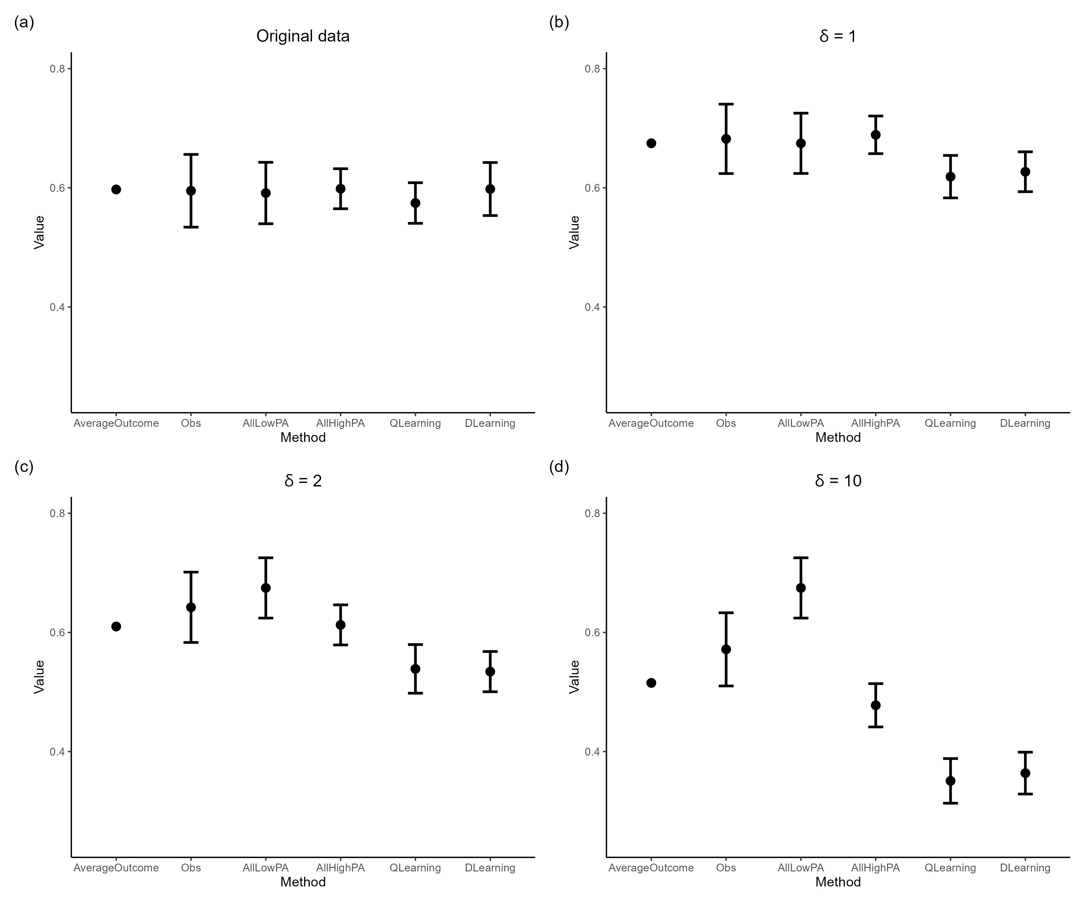
Figure 3: The value function results of six different treatment regimes: observed treatment, treatment $A=0$ for all individuals, treatment $A=1$ for all individuals, Q-learning optimal ITR, and D-learning optimal ITR. For comparison purposes, we include the average outcome as a benchmark. (a) shows the results on original data, and (b)(c)(d) shows the three simulated data with three levels of treatment effect modification $\delta=1$, $\delta=2$, $\delta=10$, respectively.

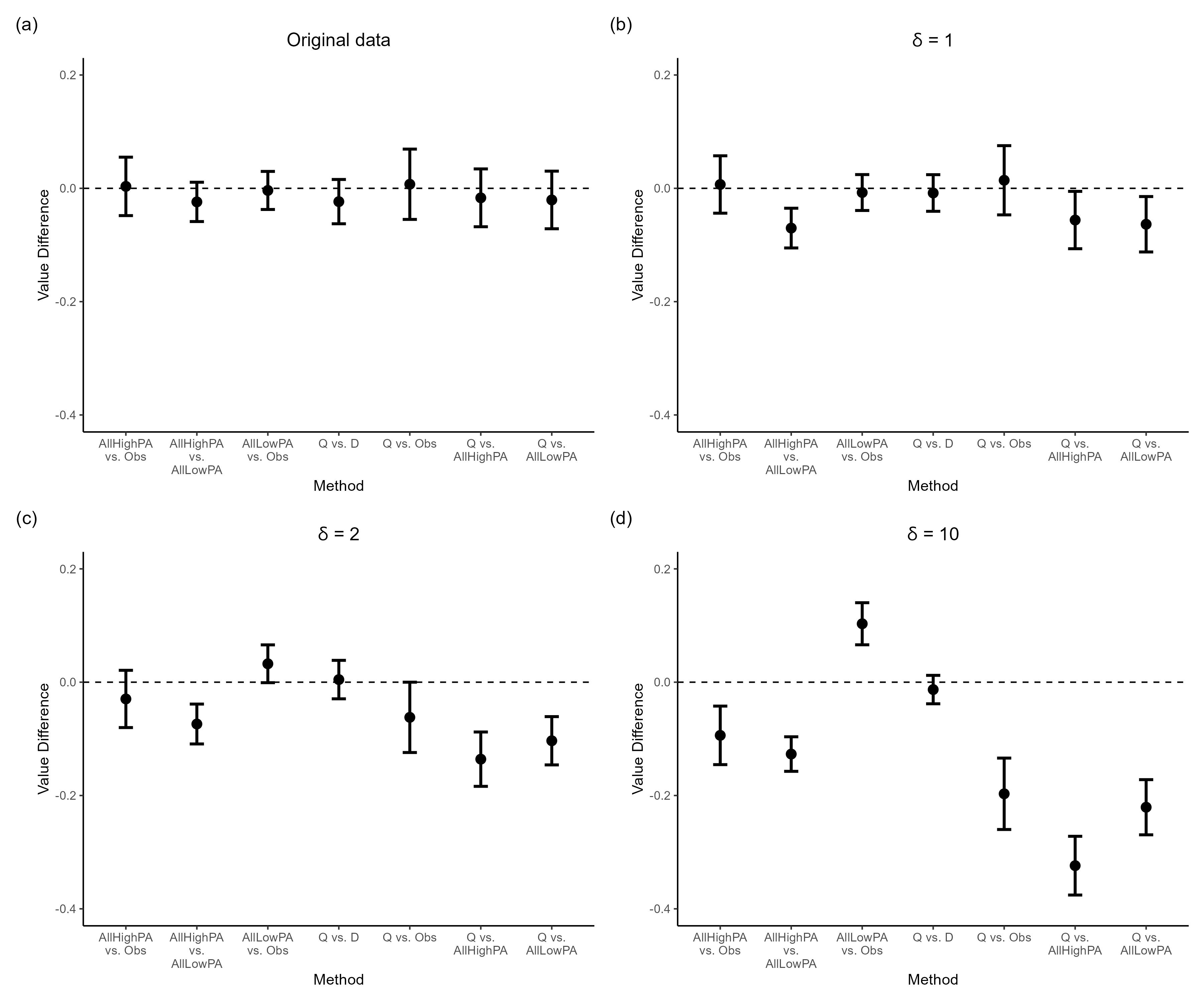
Figure 4: The value function differences among selected pairs of treatment regimes. Specifically, the Q-learning optimal ITR comparison with the observed treatment, treatment $A=0$ for all individuals, treatment $A=1$ for all individuals, and D-learning optimal ITR are shown. (a) shows the results on original data, and (b)(c)(d) shows the three simulated data with three levels of treatment effect modification $\delta=1$, $\delta=2$, $\delta=10$, respectively.

The data was split into a 70% training set and a 30% test set, with missForest imputation performed 10 times on each set to avoid dependency. We obtained Q-learning optimal ITRs ⁴ and D-learnings optimal ITR ⁵ for each of the training sets using a logistic regression model with elastic-net penalization. We then compared the value function of each treatment rule on the test set, including the observed treatment, assigning all individuals to treatment $A=1$ or $A=0$, optimal ITRs derived from Q-learning and D-learning. The value functions of these treatment rules were estimated using the common estimator $V$ and the differences between value functions were directly obtained by subtracting the value functions and then averaged over 10 imputed data sets. The variance of the value function and the variance of the difference between the value functions were estimated by our method, which accounts for both modeling and multiple imputation variance.

Table 3: Estimated value functions of different treatment regimes for CHNS data.

	Training Set		Test Set
	Mean	SD	Mean	SD
Obs	0.602	0.021	$0.595$	0.031
AllLowPA	0.603	0.018	$0.591$	0.026
AllHighPA	0.600	0.011	$0.598$	0.017
Q-Learning	0.568	0.013	$0.574$	0.017
D-Learning	0.576	0.016	$0.598$	0.023

Table 4: Estimated value differences and p-values of selected comparisons between treatment regimes for CHNS data.

	Training Set			Test Set
Difference	Mean	SD	P-Value	Mean	SD	P-Value
AllLowPA vs. Obs	0.001	0.011	0.924	-0.004	0.017	0.827
AllHighPA vs. Obs	-0.001	0.018	0.953	0.003	0.026	0.897
AllHighPA vs. AllLowPA	-0.002	0.021	0.921	0.007	0.032	0.821
Q vs. Obs	-0.033	0.017	0.046	-0.021	0.026	0.429
Q vs. AllLowPA	-0.034	0.017	0.040	-0.017	0.026	0.519
Q vs. AllHighPA	-0.032	0.013	0.014	-0.024	0.018	0.176
Q vs. D	-0.008	0.013	0.562	-0.023	0.020	0.239

Our goal is to compare personalized and uniform interventions in reducing hypertension risk by comparing the value functions in test sets for (1) observed physical activity, under the assumption that individuals continue their existing routines; (2) assigning all individuals to treatment $A=1$, assuming all individuals are above the 5 hours weekly MVPA recommendation; (3) assigning all individuals to treatment $A=0$, assuming all individuals are at or below the 5 hours weekly MVPA recommendation; and (4) optimal ITRs derived from various methods. Figure 3(a) shows the value function and variances for those treatment regimes. The Q-learning value function is the lowest. This means that if the population follows the Q-learning ITR, the expected risk of hypertension in the population is lower than that if the population follows the other treatment assignment, although the differences between the value functions are small. Figure 4(a) shows the pairwise difference of the value functions between treatment regimes that we are interested in. Our focus is on determining the necessity of recommending over 5 hours of weekly MVPA to everyone or specific subgroups. Thus we compare the best ITR, Q-learning ITR, defined by the lowest value function estimate in the training set (Table 3) with the one-size-fits-all treatment $A=1$ for the test set. Based on the t-test result, the value functions are not significantly different, with a p-value of 0.18 for the Q-learning personalized treatment rule compared to assigning all individuals to treatment $A=1$ (Table 4). This suggests that a personalized approach does not significantly outperform the population-level physical activity recommendations for doing physical activity for more than five hours per week. Although the training data results show that the Q-learning has a significantly lower value function than the best one-size-fits-all treatment $A=1$, the results shown here are test set results. The test set results hold particular significance as they underscore the model’s generalizability. They offer insight into the performance expected of the trained model when confronted with new and unseen data.

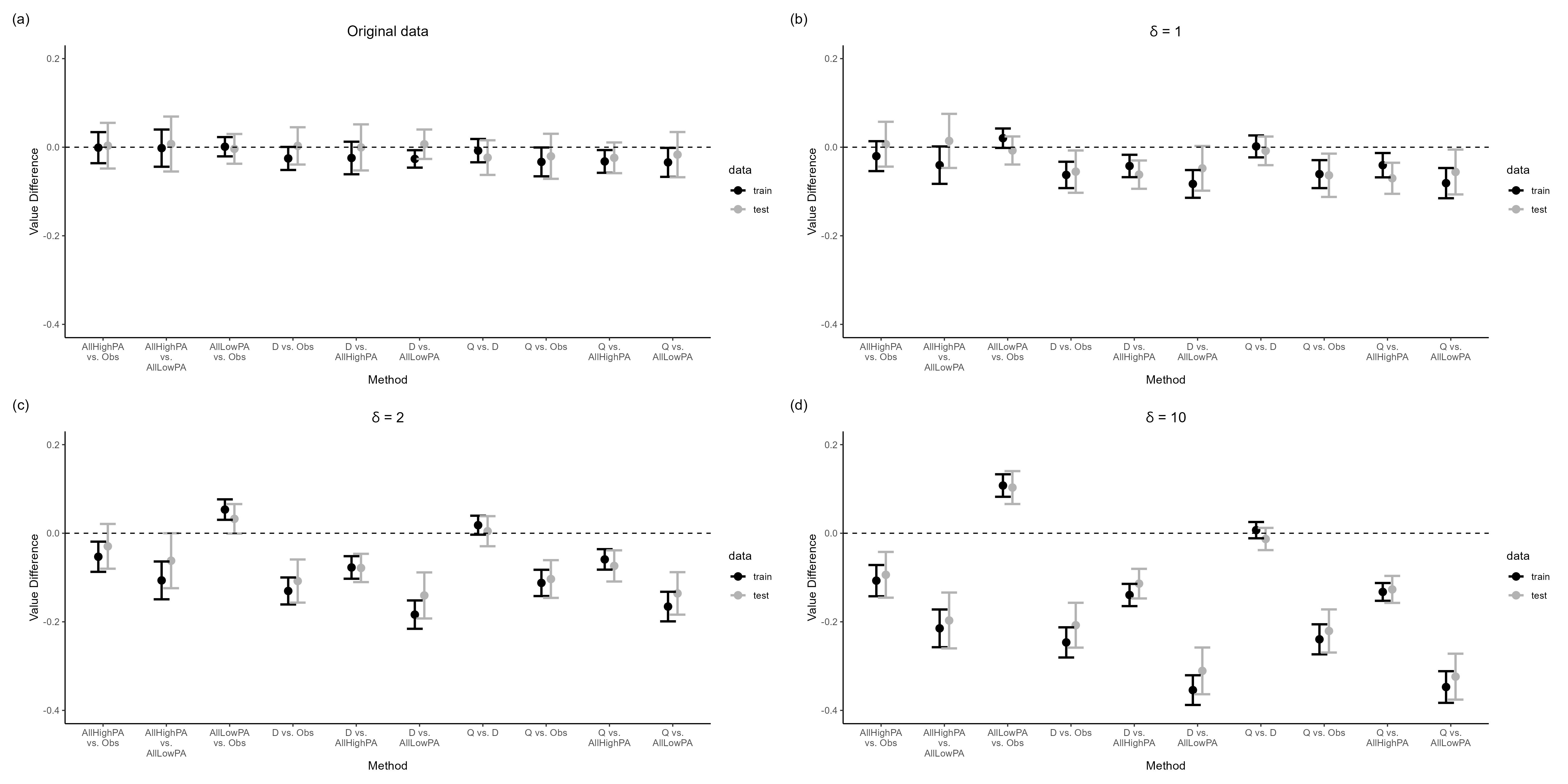
Figure 6: The differences of value functions between the pairs of the following treatments for both training and test sets: treatment $A=0$ for all individuals, treatment $A=1$ for all individuals, Q-learning optimal ITR, and D-learning optimal ITR. The results on original data (a) and three simulated data with three levels of treatment effect modification are shown (b) $\delta=1$, (c) $\delta=2$, (d) $\delta=10$.

Our findings suggest that adjustments in physical activity for a subset of individuals alone do not yield a substantial reduction in hypertension risk at the population level. Alternative non-pharmacologic interventions may demonstrate greater efficacy in mitigating hypertension risk across specific subpopulations. This variance in response may be influenced by the interaction between multiple factors, such as sodium intake and physical activity. For instance, individuals with high sodium consumption may not benefit significantly from increased physical activity alone. In contrast, sodium intake reduction could potentially offer a more effective strategy for lowering hypertension risk. Another possible explanation is that much physical activity in the CHNS data comprised working, as opposed to leisure, activities. Published data suggest that occupational physical activity may not be as protective against hypertension ³⁶. The complete pairwise comparison of all the comparisons is depicted in the appendix Figure 6.

4.2 CHNS: Augmented Analysis

These differences across all the value functions in our original CHNS analysis could truly be this small in magnitude. However, it is important to note that these models only consider a small subset of factors that could impact how changes in physical activity can impact hypertension. Hypertension is complex, resulting from an interplay between individual behavior, environment, and additional factors like metabolism and genetics. These factors might help provide additional important insight and better identify underlying heterogeneity in the impact of physical activity on hypertension not captured in our original analysis. Therefore, we wanted to investigate our method’s performance in the presence of prescriptive treatment effect interaction, which corresponds to these additional factors, or combinations of these additional factors with our existing factors, that explain more of the variation in how an individual’s hypertension risk would be impacted by changes in physical activity. Therefore, an additional analysis was carried out on simulated datasets with modified prescriptive treatment effect interaction terms.

The outcome variables in these data sets were generated by the fitted Q-learning outcome regression model with the treatment effect interaction terms (excluding the treatment main effect term) multiplied by a factor of $\delta\geq 1$. We investigate three options of $\delta$ for this analysis: $\delta=1$, $\delta=2$, and $\delta=10$, representing the estimated original, double, and tenfold treatment effect, respectively. In each analysis, hypertension outcomes are replaced by generated outcomes from the modified Q-learning outcome regression model. This augmented analysis examines our method’s performance when the outcome generative process is known and how the performance varies as the true prescriptive treatment effect enlarges.

As $\delta$ increases, from $\delta=1$, to $\delta=2$, to $\delta=10$ (Figure 3 (b)-(d)), the value function differences between the Q-learning strategy and other treatment rules increase. Figure 4 shows the difference in magnitude between the pairwise differences in value function results between the Q-learning treatment rules and both (1) assigning all individuals to either treatment $A=1$ and (2) treatment $A=0$ across our original results. The complete pairwise comparison of all the comparisons is depicted in the appendix figure 6. In all these instances, the Q-learning models deliver the best ITRs, with values notably lower, suggesting a lower risk of hypertension in the treatment-effect-augmented population especially when compared to population interventions when all individuals are assigned to low physical activity or all individuals are assigned to high physical activity. When $\delta=1$, we observe that the pattern of value functions bears resemblance to that of the original data across various methods. As the prescriptive treatment effect becomes increasingly evident, both Q-learning and D-learning demonstrate progressively superior performance compared to the ’one-size-fits-all’ approaches. This underscores the importance of personalizing over population-level interventions when certain factors significantly affect individual responses to treatment. Applying these methods to existing rich, detailed observational data can provide an important insight into factors that might distinguish these subgroups of responders. Future work will build on these existing models to better incorporate additional high-dimensional data. However, these results suggest that if a large heterogeneous effect truly exists, our method can successfully capture it.

5 Discussion

In this paper, we propose an innovative t-test based approach that can directly compare the value functions of any two treatment regimes. The validity of the approach follows from the asymptotic normality of the standard value function for the estimated treatment regime and the asymptotic normality of the propensity score model parameters. Our method provides valid estimates for (1) the variance for a value function for a single treatment regime, (2) the variance for the difference between two value functions of two treatment regimes, (3) the p-value of the t-test for the significance of the difference between two value functions, and (4) the application of these estimations in scenarios involving multiple imputations. This method maintains simplicity in variance calculation and is computationally more efficient than the bootstrap method, especially when multiple imputation is used for handling missing data. Through simulation studies and the data application example, we demonstrate the performance and the ease of implementation of our method in different scenarios. Additionally, this method enables the evaluation and comparison of ITR effectiveness using abundant observational cohort data when clinical trial data are not available. This comparison is crucial as individuals seek behavioral modification guidance amidst numerous recommendations, and emphasizing targeting strategies could increase the likelihood of effective changes.

Nevertheless, it is important to acknowledge a limitation inherent in our methodology – its reliance on the presupposition that the propensity score model holds true. In observational data, extreme propensity scores can influence the estimates of the value function as well as the variance estimates of the value function. For future work, it will be interesting to use more robust estimators to alleviate the impact of potential misspecification of the propensity score model. Another extension of this method is to multiple-stage ITR comparison. Expanding our method to simultaneously compare more than two ITRs would also present an interesting avenue for further exploration.

To conclude, our method offers a convenient approach to comparing two treatment regimes directly. Furthermore, it is suitable for observational data and randomized trial data and has the ability to incorporate multiple imputation for missing data.

Appendix A Proofs

Proof of Proposition 1

Proof.

$\sqrt{m}(\hat{V}_{m}(\hat{d}_{j,n})-V_{0}(\hat{d}_{j,n}))=$

$$\sqrt{m}(\frac{\sum_{i=1}^{m}\frac{y_{i}1\{a_{i}=\hat{d}_{j,n}(x_{i})\}}{\hat{\pi}_{n}(a_{i}|x_{i})}-mE(\frac{Y1\{A=\hat{d}_{j,n}(X)\}}{\hat{\pi}_{n}(A|X)})}{\sum_{i=1}^{m}\frac{1\{a_{i}=\hat{d}_{j,n}(x_{i})\}}{\hat{\pi}_{n}(a_{i}|x_{i})}})$$

$$-\sqrt{m}(\frac{E[\frac{Y1\{A=\hat{d}_{j,n}(X)\}}{\hat{\pi}_{n}(A|X))}][\sum_{i=1}^{n}\frac{1\{a_{i}=\hat{d}_{j,n}(x_{i})\}}{\hat{\pi}_{n}(a_{i}|x_{i})}-mE(\frac{1\{A=\hat{d}_{j,n}(X)\}}{\hat{\pi}_{n}(A|X)})]}{E[\frac{1\{A=\hat{d}_{j,n}(X)\}}{\hat{\pi}_{n}(A|X))}][\sum_{i=1}^{n}\frac{1\{a_{i}=\hat{d}_{j,n}(x_{i})\}}{\hat{\pi}_{n}(a_{i}|x_{i})}]})$$

$$+\sqrt{m}\left(\frac{E[\frac{Y1\{A=\hat{d}_{j,n}(X)\}}{\hat{\pi}_{n}(A|X))}]-E[\frac{Y1\{A=\hat{d}_{j,n}(X)\}}{\pi_{0}(A|X))}]}{E[\frac{1\{A=\hat{d}_{j,n}(X)\}}{\hat{\pi}_{n}(A|X))}]}\right)$$

$$-\sqrt{m}(\frac{E[\frac{Y1\{A=\hat{d}_{j,n}(X)\}}{\pi_{0}(A|X))}][E[\frac{1\{A=\hat{d}_{j,n}(X\}}{\hat{\pi}_{n}(A|X)}-E(\frac{1\{A=\hat{d}_{j,n}(X)\}}{\pi_{0}(A|X)})]}{E[\frac{1\{A=\hat{d}_{j,n}(X)\}}{\hat{\pi}_{n}(A|X))}]E[\frac{1\{A_{=}\hat{d}_{j,n}(X)\}}{\pi_{0}(A|X)}]})$$

$$=B_{1,m}-B_{2,m}+B_{3,m}-B_{4,m},$$

where

$$B_{1,m}=\sqrt{m}(\frac{\sum_{i=1}^{m}\frac{y_{i}1\{a_{i}=\hat{d}_{j,n}(x_{i})\}}{\hat{\pi}_{n}(a_{i}|x_{i})}-mE(\frac{Y1\{A=\hat{d}_{j,n}(X)\}}{\hat{\pi}_{n}(A|X)})}{\sum_{i=1}^{m}\frac{1\{a_{i}=\hat{d}_{j,n}(x_{i})\}}{\hat{\pi}_{n}(a_{i}|x_{i})}})$$

$$=\frac{\mathbb{G}_{n}(\frac{Y1\{A=\hat{d}_{j,n}(X)\}}{\hat{\pi}_{n}(A|X)})}{\mathbb{P}_{n}[\frac{1\{A=\hat{d}_{j,n}(X)\}}{\hat{\pi}_{n}(A|X)}]}=\mathbb{G}_{n}[\frac{Y1\{A=\hat{d}_{j,n}(X)\}}{\pi_{0}(A|X)}]+o_{P}(1),$$

where $\mathbb{G}_{n}((f(U))=\sqrt{n}[\mathbb{P}_{n}(f(U))-P(f(U))]$, $\mathbb{P}_{n}f(U)=n^{-1}\sum_{i=1}^{n}f(u_{i})$ is the empirical measure, $Pf(U)=E(f(U))$ is the expectation taken over $U$. By empirical process methods, $\mathbb{P}_{n}[\frac{1\{A=\hat{d}_{j,n}(X)\}}{\hat{\pi}_{n}(A|X)}]\rightarrow E[\frac{1\{A=\hat{d}_{j,n}(X)\}}{\pi_{0}(A|X)}]=1$, in probability. Using Slutsky’s theorem, and the empirical average converges to its limiting value.

Next,

$$B_{2,m}=\frac{E[\frac{Y1\{A=\hat{d}_{j,n}(X)\}}{\hat{\pi}_{n}(A|X)}]\mathbb{G}_{n}[\frac{1\{A=\hat{d}_{j,n}(X)\}}{\hat{\pi}_{n}(A|X)}]}{E[\frac{1\{A=\hat{d}_{j,n}(X)\}}{\hat{\pi}_{n}(A|X)}]\mathbb{P}_{n}[\frac{1\{A=\hat{d}_{j,n}(X)\}}{\hat{\pi}_{n}(A|X)}]}=V_{0}(\hat{d}_{j,n})\mathbb{G}_{n}(\frac{1\{A=\hat{d}_{j,n}(X)\}}{\pi_{0}(A|X)})+o_{P}(1),$$

by the following steps based on empirical process methods and Slutsky’s theorem:

$$\frac{E[\frac{Y1\{A=\hat{d}_{j,n}(X)\}}{\hat{\pi}_{n}(A|X)}]}{E[\frac{1\{A=\hat{d}_{j,n}(X)\}}{\hat{\pi}_{n}(A|X)}]}=\frac{E[\frac{Y1\{A=\hat{d}_{j,n}(X)\}}{\pi_{0}(A|X)}]}{E[\frac{1\{A=\hat{d}_{j,n}(X)\}}{\pi_{0}(A|X)}]}+o_{P}(1)=V_{0}(\hat{d}_{j,n})+o_{P}(1),$$

$$\mathbb{P}_{n}[\frac{1\{A=\hat{d}_{j,n}(X)\}}{\hat{\pi}_{n}(A|X)}]=1+o_{P}(1),$$

$$\mathbb{G}_{n}[\frac{1\{A=\hat{d}_{j,n}(X)\}}{\hat{\pi}_{n}(A|X)}]=\mathbb{G}_{n}[\frac{1\{A=\hat{d}_{j,n}(X)\}}{\pi_{0}(A|X)}]+o_{P}(1).$$

Next,

$$B_{3,m}=\sqrt{m}\left(\frac{E[\frac{Y1\{A=\hat{d}_{j,n}(X)\}}{\hat{\pi}_{n}(A|X))}]-E[\frac{Y1\{A=\hat{d}_{j,n}(X)\}}{\pi_{0}(A|X))}]}{E[\frac{1\{A=\hat{d}_{j,n}(X)\}}{\hat{\pi}_{n}(A|X))}]}\right)$$

$$=\frac{E[Y1\{A=\hat{d}_{j,n}(X)\}]E[\sqrt{m}(\frac{1}{\hat{\pi}_{n}(A|X)}-\frac{1}{\pi_{0}(A|X)})]}{E[\frac{1\{A=\hat{d}_{j,n}(X)\}}{\hat{\pi}_{n}(A|X)}]}$$

$$=-E[\frac{Y1\{A=\hat{d}_{j,n}(X)\}\sqrt{m}(\hat{\pi}_{n}(A|X)-\pi_{0}(A|X))}{\pi^{2}_{0}(A|X)}]+o_{P}(1).$$

Since $\sqrt{n}(\pi(a|x,\hat{\theta}_{n})-\pi(a|x,\theta_{0}))=\sqrt{n}(\hat{\theta}_{n}-\theta_{0})^{T}\phi_{0}(a,x)+o_{p}(1)$, we now have that

$$B_{3,m}=-\sqrt{m/n}*\sqrt{n}(\hat{\theta}_{n}-\theta_{0})^{T}E[\phi_{0}(A,X)\frac{Y1\{A=\hat{d}_{j,n}(X)\}}{\pi_{0}^{2}(A|X)}]+o_{P}(1).$$

Finally,

$$B_{4,m}=-\sqrt{m}\frac{E(\frac{Y1\{A=\hat{d}_{j,n}(X)\}}{\pi_{0}(A|X)})E[1\{A=\hat{d}_{j,n}(X)\}(\frac{1}{\hat{\pi}_{n}(A|X)}-\frac{1}{\pi_{0}(A|X)})]}{E(\frac{1\{A=\hat{d}_{j,n}(X)\}}{\pi_{0}(A|X)})E(\frac{1\{A=\hat{d}_{j,n}(X)\}}{\hat{\pi}_{n}(A|X)})}$$

$$=-V_{0}(\hat{d}_{j,n})E[1\{A=\hat{d}_{j,n}(X)\}\sqrt{m}(\frac{1}{\hat{\pi}_{n}(A|X)}-\frac{1}{\pi_{0}(A|X)})]+o_{P}(1)$$

$$=V_{0}(\hat{d}_{j,n})E[\frac{1\{A=\hat{d}_{j,n}(X)\}}{\pi_{0}^{2}(A|X)}\sqrt{m}(\hat{\pi}_{n}(A|X)-\pi_{0}(A|X))]+o_{P}(1)$$

$$=\sqrt{m/n}\sqrt{n}(\hat{\theta}_{n}-\theta_{0})^{T}E[\phi_{0}(A,X)\frac{1\{A=\hat{d}_{j,n}(X)\}}{\pi_{0}^{2}(A|X)}]V_{0}(\hat{d}_{j,n})+o_{P}(1).$$

Thus:

$$\sqrt{m}(\hat{V}_{m}(\hat{d}_{j,n})-V_{0}(\hat{d}_{j,n})) =\mathbb{G}_{m}(\frac{Y1\{A=\hat{d}_{j,n}(X)\}}{\pi_{0}(A|X)})$$

$$-V_{0}(\hat{d}_{j,n})\mathbb{G}_{m}(\frac{1\{A=\hat{d}_{j,n}(X)\}}{\pi_{0}(A|X)})$$

$$-\sqrt{m/n}\sqrt{n}(\hat{\theta}_{n}-\theta_{0})^{T}E[\phi_{0}(A|X)\frac{Y1\{A=\hat{d}_{j,n}(X)\}}{\pi^{2}_{0}(A|X)}]$$

$$+\sqrt{m/n}\sqrt{n}(\hat{\theta}_{n}-\theta_{0})^{T}E[\phi_{0}(A|X)\frac{1\{A=\hat{d}_{j,n}(X)\}}{\pi^{2}_{0}(A|X)}]V_{0}(\hat{d}_{j,n})+o_{P}(1)$$

$$=\mathbb{G}_{m}(\frac{(Y-V_{0}(\hat{d}_{j,n}))1\{A=\hat{d}_{j,n}(X)\}}{\pi_{0}(A|X)})$$

$$-\sqrt{m/n}\sqrt{n}(\hat{\theta}_{n}-\theta_{0})^{T}E(\phi_{0}(A,X)\frac{(Y-V_{0}(\hat{d}_{j,n}))1\{A=\hat{d}_{j,n}(x)\}}{\pi^{2}_{0}(A|X)})+o_{P}(1),$$

and the desired results follow. ∎

Proof of Proposition 2

Proof.

$$\sqrt{m}(\hat{V}_{m}(\hat{d}_{1,n})-\hat{V}_{m}(\hat{d}_{2,n})-V_{0}(\hat{d}_{1,n})+V_{0}(\hat{d}_{2,n}))$$

$$=\mathbb{G}_{m}[\frac{(Y-V_{0}(\hat{d}_{1,n}))1\{A=\hat{d}_{1,n}(x)\}-(Y-V_{0}(\hat{d}_{2,n}))1\{A=\hat{d}_{2,n}(x)\}}{\pi_{0}(A|X)}]$$

$$-\sqrt{m/n}\sqrt{n}(\hat{\theta}_{n}-\theta_{0})^{T}E(\phi_{0}(A,X)\frac{(Y-V_{0}(\hat{d}_{1,n}))1\{A=\hat{d}_{1,n}(x)\}-(Y-V_{0}(\hat{d}_{2,n}))1\{A=\hat{d}_{2,n}(x)\}}{\pi_{0}^{2}(A|X)})+o_{P}(1)$$

$$\rightarrow N(0,T_{0}^{2}),$$

in distribution, and standard arguments can now be used to show that $\hat{T}_{m}^{2}\rightarrow T_{0}^{2}$ as $m\rightarrow\infty$, where

$$\hat{T}_{m}^{2}=m^{-1}\sum_{i=1}^{m}(\hat{U}_{i,1}-\hat{U}_{i,2}-\bar{U}_{m,1}+\bar{U}_{m,2})^{2}+m(\hat{W}_{m,1}-\hat{W}_{m,2})^{T}\hat{\Sigma}_{n}(\hat{W}_{m,1}-\hat{W}_{m,2}).$$

∎

Appendix B Additional Figures

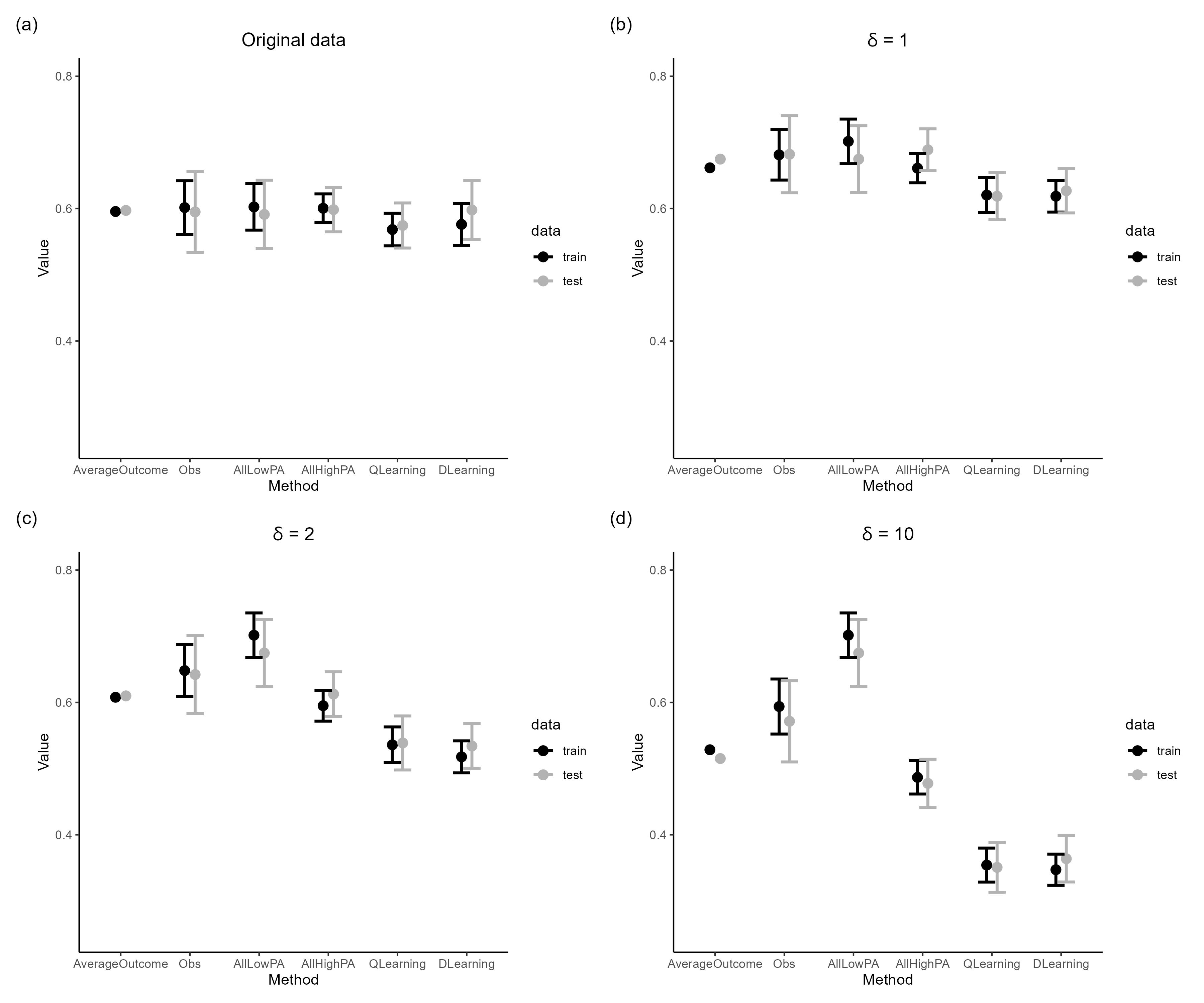
Figure 5: The value function results for both training and test sets for five different treatment regimes: observed treatment, treatment $A=0$ for all individuals, treatment $A=1$ for all individuals, Q-learning optimal ITR, and D-learning optimal ITR. For comparison purposes, we include the average outcome as a benchmark. The results on original data (a) and three simulated data sets with three levels of treatment effect modification are shown (b) $\delta=1$, (c) $\delta=2$, (d) $\delta=10$.

References

- Piercy et al. 2018 Katrina L Piercy, Richard P Troiano, Rachel M Ballard, Susan A Carlson, Janet E Fulton, Deborah A Galuska, Stephanie M George, and Richard D Olson. The physical activity guidelines for americans. Jama, 320(19):2020–2028, 2018.
- Olson et al. 2019 Richard D Olson, Katrina L Piercy, Richard P Troiano, Rachel M Ballard, Janet E Fulton, Deborah A Galuska, Shellie Y Pfohl, Alison Vaux-Bjerke, Julia B Quam, Stephanie M George, Kyle Sprow, Susan A Carlson, Eric T Hyde, and Kate Olscamp. Physical Activity Guidelines for Americans 2nd edition. The U.S. Department of Health and Human Services, https://health.gov/sites/default/files/2019-09/Physical_Activity_Guidelines_2nd_edition.pdf, 2019.
- Bouchard and Rankinen 2001 Claude Bouchard and Tuomo Rankinen. Individual differences in response to regular physical activity. Medicine & Science in Sports & Exercise, 33(6):S446–S451, 2001.
- Qian and Murphy 2011 Min Qian and Susan A Murphy. Performance guarantees for individualized treatment rules. Annals of statistics, 39(2):1180, 2011.
- Tian et al. 2014 Lu Tian, Ash A Alizadeh, Andrew J Gentles, and Robert Tibshirani. A simple method for estimating interactions between a treatment and a large number of covariates. Journal of the American Statistical Association, 109(508):1517–1532, 2014.
- Sterne et al. 2009 Jonathan AC Sterne, Ian R White, John B Carlin, Michael Spratt, Patrick Royston, Michael G Kenward, Angela M Wood, and James R Carpenter. Multiple imputation for missing data in epidemiological and clinical research: potential and pitfalls. Bmj, 338, 2009.
- Jiang et al. 2021 Xiaotong Jiang, Amanda E Nelson, Rebecca J Cleveland, Daniel P Beavers, Todd A Schwartz, Liubov Arbeeva, Carolina Alvarez, Leigh F Callahan, Stephen Messier, Richard Loeser, et al. Precision medicine approach to develop and internally validate optimal exercise and weight-loss treatments for overweight and obese adults with knee osteoarthritis: data from a single-center randomized trial. Arthritis care & research, 73(5):693–701, 2021.
- Cui et al. 2017 Yifan Cui, Ruoqing Zhu, and Michael Kosorok. Tree based weighted learning for estimating individualized treatment rules with censored data. Electronic journal of statistics, 11(2):3927, 2017.
- Zhao et al. 2012 Yingqi Zhao, Donglin Zeng, A John Rush, and Michael R Kosorok. Estimating individualized treatment rules using outcome weighted learning. Journal of the American Statistical Association, 107(499):1106–1118, 2012.
- Efron 1992 Bradley Efron. Bootstrap methods: another look at the jackknife. In Breakthroughs in statistics: Methodology and distribution, pages 569–593. Springer, 1992.
- Shi et al. 2022 Chengchun Shi, Sheng Zhang, Wenbin Lu, and Rui Song. Statistical inference of the value function for reinforcement learning in infinite-horizon settings. Journal of the Royal Statistical Society Series B: Statistical Methodology, 84(3):765–793, 2022.
- Bates et al. 2021 Stephen Bates, Trevor Hastie, and Robert Tibshirani. Cross-validation: what does it estimate and how well does it do it? arXiv preprint arXiv:2104.00673, 2021.
- Chakraborty et al. 2010 Bibhas Chakraborty, Susan Murphy, and Victor Strecher. Inference for non-regular parameters in optimal dynamic treatment regimes. Statistical methods in medical research, 19(3):317–343, 2010.
- Laber and Murphy 2011 Eric B Laber and Susan A Murphy. Adaptive confidence intervals for the test error in classification. Journal of the American Statistical Association, 106(495):904–913, 2011.
- Chakraborty et al. 2013 Bibhas Chakraborty, Eric B Laber, and Yingqi Zhao. Inference for optimal dynamic treatment regimes using an adaptive m-out-of-n bootstrap scheme. Biometrics, 69(3):714–723, 2013.
- Austin 2011 Peter C Austin. An introduction to propensity score methods for reducing the effects of confounding in observational studies. Multivariate behavioral research, 46(3):399–424, 2011.
- Van Buuren 2018 Stef Van Buuren. Flexible imputation of missing data. CRC press, 2018.
- Zou and Hastie 2005 Hui Zou and Trevor Hastie. Regularization and variable selection via the elastic net. Journal of the royal statistical society: series B (statistical methodology), 67(2):301–320, 2005.
- Bloch 2016 Michael J Bloch. Worldwide prevalence of hypertension exceeds 1.3 billion. Journal of the American Society of Hypertension: JASH, 10(10):753–754, 2016.
- Bromfield and Muntner 2013 Samantha Bromfield and Paul Muntner. High blood pressure: the leading global burden of disease risk factor and the need for worldwide prevention programs. Current hypertension reports, 15:134–136, 2013.
- Weldegiorgis and Woodward 2020 Misghina Weldegiorgis and Mark Woodward. The impact of hypertension on chronic kidney disease and end-stage renal disease is greater in men than women: a systematic review and meta-analysis. BMC nephrology, 21(1):1–9, 2020.
- Bhargava et al. 2012 M Bhargava, MK Ikram, and Tien Yin Wong. How does hypertension affect your eyes? Journal of human hypertension, 26(2):71–83, 2012.
- Kilander et al. 1998 Lena Kilander, Hakan Nyman, Merike Boberg, Lennart Hansson, and Hans Lithell. Hypertension is related to cognitive impairment: a 20-year follow-up of 999 men. Hypertension, 31(3):780–786, 1998.
- Wang et al. 2017 Guijing Wang, Xilin Zhou, Xiaohui Zhuo, and Ping Zhang. Annual total medical expenditures associated with hypertension by diabetes status in us adults. American journal of preventive medicine, 53(6):S182–S189, 2017.
- Zhang et al. 2023 Mei Zhang, Yu Shi, Bin Zhou, Zhengjing Huang, Zhenping Zhao, Chun Li, Xiao Zhang, Guiyuan Han, Ke Peng, Xinhua Li, et al. Prevalence, awareness, treatment, and control of hypertension in china, 2004-18: findings from six rounds of a national survey. bmj, 380, 2023.
- Wang et al. 2023 Ji-Guang Wang, Wei Zhang, Yan Li, and Lisheng Liu. Hypertension in china: epidemiology and treatment initiatives. Nature Reviews Cardiology, pages 1–15, 2023.
- Cui et al. 2020 Bin Cui, Zhaohui Dong, Mengmeng Zhao, Shanshan Li, Hua Xiao, Zhitao Liu, and Xiaowei Yan. Analysis of adherence to antihypertensive drugs in chinese patients with hypertension: a retrospective analysis using the china health insurance association database. Patient preference and adherence, pages 1195–1204, 2020.
- Appel 2003 Lawrence J Appel. Lifestyle modification as a means to prevent and treat high blood pressure. Journal of the American Society of Nephrology, 14(suppl 2):S99–S102, 2003.
- Cane et al. 2012 James Cane, Denise O’Connor, and Susan Michie. Validation of the theoretical domains framework for use in behaviour change and implementation research. Implementation science, 7:1–17, 2012.
- Zhang et al. 2014 Bing Zhang, FY Zhai, SF Du, and Barry M Popkin. The c hina h ealth and n utrition s urvey, 1989–2011. Obesity reviews, 15:2–7, 2014.
- Ng et al. 2014 Shu Wen Ng, A-G Howard, HJ Wang, Chang Su, and Bing Zhang. The physical activity transition among adults in c hina: 1991–2011. Obesity Reviews, 15:27–36, 2014.
- Ainsworth et al. 2011 Barbara E Ainsworth, William L Haskell, Stephen D Herrmann, Nathanael Meckes, David R Bassett Jr, Catrine Tudor-Locke, Jennifer L Greer, Jesse Vezina, Melicia C Whitt-Glover, and Arthur S Leon. 2011 compendium of physical activities: a second update of codes and met values. Medicine & science in sports & exercise, 43(8):1575–1581, 2011.
- Sylvia et al. 2014 Louisa G Sylvia, Emily E Bernstein, Jane L Hubbard, Leigh Keating, and Ellen J Anderson. A practical guide to measuring physical activity. Journal of the Academy of Nutrition and Dietetics, 114(2):199, 2014.
- Stekhoven 2022 Daniel J. Stekhoven. missForest: Nonparametric Missing Value Imputation using Random Forest. CRAN, https://cran.r-project.org/package=missForest, 2022. R package version 1.5.
- Stekhoven and Buehlmann 2012 Daniel J. Stekhoven and Peter Buehlmann. Missforest - non-parametric missing value imputation for mixed-type data. Bioinformatics, 28(1):112–118, 2012.
- Huai et al. 2013 Pengcheng Huai, Huanmiao Xun, Kathleen Heather Reilly, Yiguan Wang, Wei Ma, and Bo Xi. Physical activity and risk of hypertension: a meta-analysis of prospective cohort studies. Hypertension, 62(6):1021–1026, 2013.