Fitting neutrino flares: Applying expectation maximization on neutrino data
Abstract
We present a new approach for identifying neutrino flares. Using the unsupervised machine learning algorithm expectation maximization, we reduce computing times compared to conventional approaches by a factor of on a single CPU. Expectation maximization is also easily expandable to multiple flares. We explain the application of the algorithm and fit the neutrino flare of TXS 0506+056 as an example.
1 Introduction
In September 2018, the IceCube Neutrino Observatory [1] detected a high-energetic neutrino that led to the first identification of the blazar TXS 0506+056 as a cosmic neutrino source [2]. Furthermore, there is evidence for transient neutrino emission between 2014 and 2015 from the same direction [3, 4, 5]. This motivates the search for transient neutrino emission from other source candidates or even the whole sky.
Conventional methods for identifying neutrino flares as in references [3, 4, 6, 7] calculate signal weights for each event and apply brute force scans where all possible intervals of events with weights exceeding a certain threshold are either evaluated as possible starting and end times of a neutrino flare or used as a seed for subsequent optimization of parameters. In ref. [3], the threshold was very small, i.e., all events better described by the signal hypothesis than the background hypothesis were identified as possible starting and endpoints. Adopting this approach leads to immense computing times. Especially since the available IceCube (or neutrino data in general with new neutrino telescopes in construction) keeps increasing, running expensive searches on large sections of the sky on 10+ years of neutrino data becomes more and more computationally infeasible.
Increasing the signal weight threshold is one way to reduce the computing time. However, this also means evaluating reduced information and potentially favoring assumed source spectral indices since the assumed source spectral index enters the signal weight calculation.
We investigated new approaches in ref. [8, 9] and conducted a first search applying an unsupervised machine learning algorithm on IceCube data in ref. [10, 5, 9]. We present this new method in detail and apply it to neutrino data to identify the neutrino flare of TXS 0506+056. For this, we use published data of through-going muon-tracks [11] of the IceCube Neutrino Observatory with the open source framework SkyLLH111https://github.com/icecube/skyllh [12].
2 Identifying neutrino flares
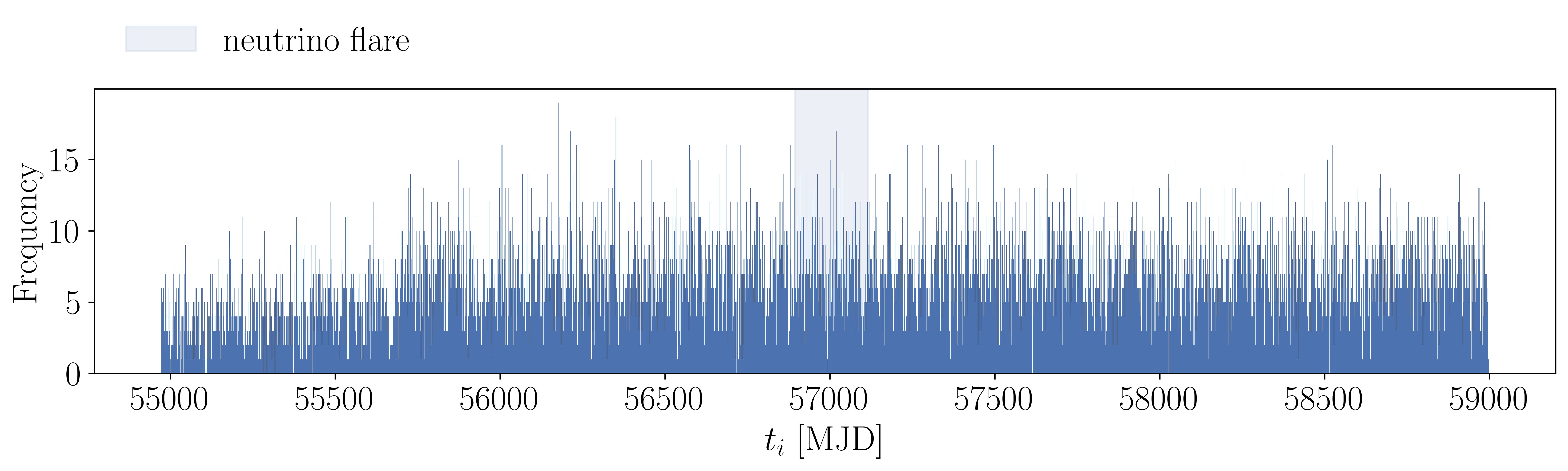
Identifying neutrino flares is challenging because neutrino data are background dominated. In Figure 1, we show the simulated event arrival times as a histogram with an additional five signal neutrinos simulated in the highlighted time range. We cannot recognize the signal by eye.
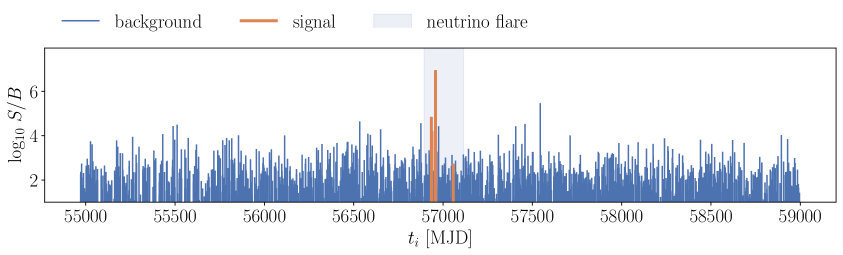
To better gauge which events are most likely relevant for the neutrino signal, we weigh each event with a “Signal over Background” factor (). For this, we evaluate the probability of an event being “signal-like” versus its probability of being “background-like”. In general, we define signal and background hypotheses as the following:
-
•
Background hypothesis : The neutrino data contains atmospheric neutrinos, atmospheric muons, and diffuse astrophysical neutrinos. We assume a uniform flux in time and right ascension222Due to IceCube’s unique position at the Sout Pole, we expect a uniform spatial background distribution in right ascension for integration times longer than a day..
-
•
Signal hypothesis : The neutrino data contains an additional signal component to the background. We assume these signal neutrinos originate from a point-like source and cluster around their source (subscript ) in right ascension and declination . Furthermore, we assume an energy spectrum following an unbroken power law: . And: the signal component is transient (time-dependent) and follows either a Gaussian time profile (with mean and width ) or a box profile with constant emission during a flare window with starting and end time (, ).
Based on these hypotheses, we define probability density functions (pdfs) as in [12]. We divide these pdfs into spatial, energy, and temporal parts. For generalization, we refer to the temporal parameters as and , which will be either and for the Gaussian profile or , for the box profile. For the signal component, we get
| (2.1) |
with as the detector’s point-spread-function (PSF) for a source at declination in the form of a two-dimensional Gaussian. defines the probability to observe an event with reconstructed energy originating from and an emission following . As emphasized in [12], the energy pdf differs from the pdfs used in internal IceCube analyses. describes the probability of observing an event at time if the source only emits during a neutrino flare described either by a Gaussian time profile centered at mean with width or a box profile with constant emission between times and .
In most cases, we do not know when we expect the source to flare. Hence, we evaluate how well the spatial and energy signal and background expectations describe each event. We calculate the “Signal over Background” () ratio as
| (2.2) |
The background descriptions are data-driven and depend on the published effective areas, and reconstruction properties [11]. Taking the simulated data, we calculate the event weights as in equation 2.2 and get the distribution in Figure 2.
2.1 Expectation Maximization
We present expectation maximization (EM) [13] as a new method to identify neutrino flares. Expectation maximization is an unsupervised learning algorithm based on Gaussian mixture models. A set of Gaussian distributions describes observed data points. has to be defined in advance and the mean values and widths of each distribution are optimized. The Gaussians can be multivariate, hence this approach works for -dimensional data.
The general description is [14]:
Expectation step
We calculate the probability for each data point, , to belong to a Gaussian distribution . The estimated parameters are:
-
•
: the means
-
•
: the covariance matrices (with dimension )
-
•
: the probabilities for each data point of , also called the responsibility matrix (the responsibility of component for data point ).
is the probability that a random data point “belongs” to Gaussian or, in different words, is the fraction of all data points originating from .
The likelihood is the product of the probabilities of observing a data point at its observed position
| (2.3) |
The Gaussian contributions of are
| (2.4) |
with as the Gaussian distribution with mean and standard deviation . is the fraction of all data points in and can also be interpreted as the number of neutrinos in a flare .
The probabilities for each data point to belong to distribution are
| (2.5) |
With these equations, it is possible to calculate and the responsibility matrix , knowing , and . This is called the expectation step (E-step).
Maximization step
The maximization step calculates , and :
| (2.6) |
| (2.7) |
and thus
| (2.8) |
Procedure
The EM algorithm is as follows:
-
1.
Guess starting values for , and .
-
2.
Repeat:
-
•
E-step to calculate new , and new
-
•
M-step to determine new , and .
-
•
-
3.
Stop when has converged.
The stopping criteria are either 500 iterations or no change of the likelihood in the past 20 iterations.
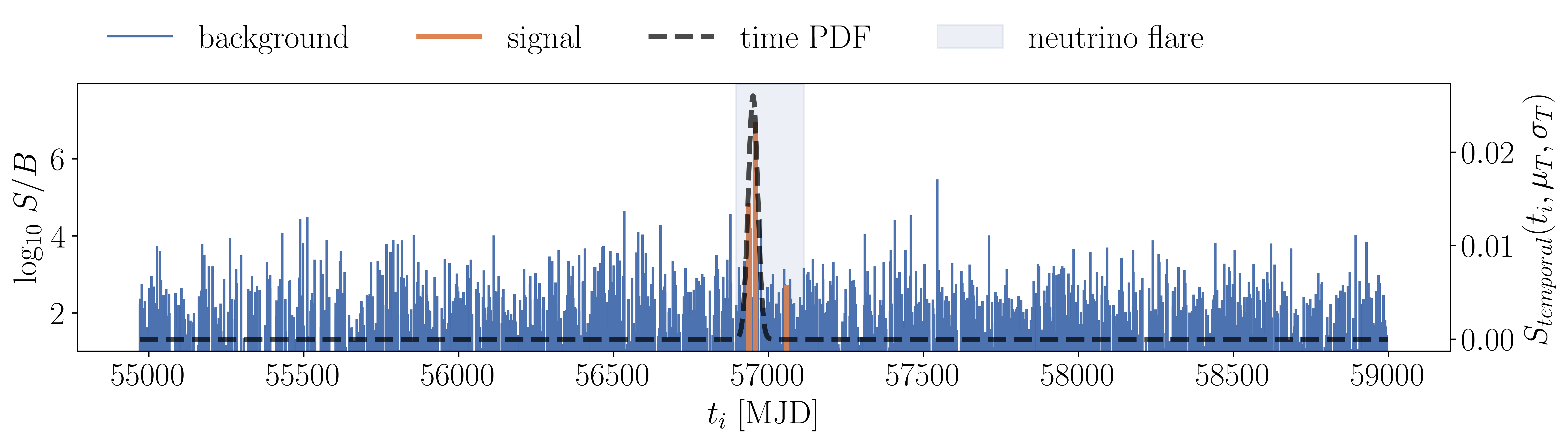
Example
We have one-dimensional data for the previous example of a single flare in a time series (). We look for now only for a single flare, hence . Considering the defined signal and background hypotheses, the model is a mixture of a Gaussian (signal) and a uniform background distribution. Hence we note as the mean flaring time, as the flare width, and as the time event was detected.
The probability of observing a data point for a mixture model of a uniform background distribution, , and a Gaussian distribution is
| (2.9) |
The expected signal with neutrinos is
| (2.10) |
with as the product of the energy and spatial pdfs as in equation 2.2. The temporal pdf is a Gaussian, .
Similarly, the background is
| (2.11) |
Here, as the product of the spatial and energy background pdfs as in equation 2.2 and .
Mixing the signal and background contributions, the responsibility matrix becomes
| (2.12) |
We use the above expressions to fit the simulated neutrino flare with EM. Comparing the best-fit temporal pdf with the simulated signal, the best-fit temporal pdf includes the significant simulated events. There is one signal event that is not included in the best-fit Gaussian shape with a relatively background-like ratio (see Figure 3).
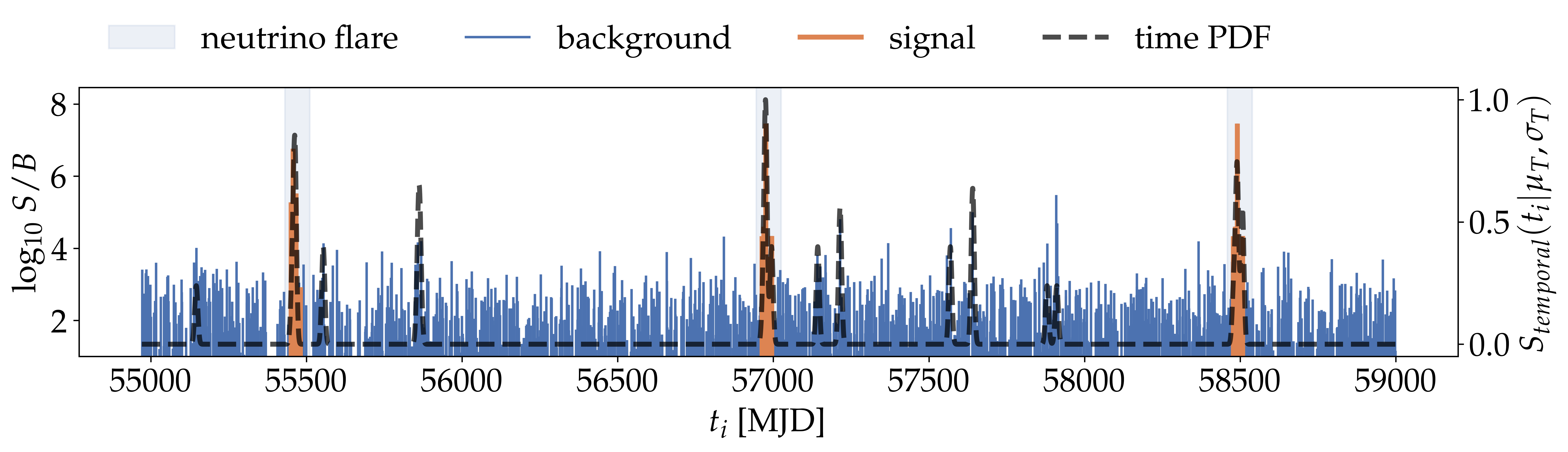
EM is easily expandable to find multiple flares. For multiple flares, we set and evaluate the Gaussian mixture model. In the following example, we simulate three flares with 5 events each and a width of days. We set since, for real data, we would not know how many flares we expect. Most flares are fit to 0. EM finds the simulated flares and also fits some background fluctuations as less significant flares, as shown in Figure 4.
2.2 Fitting the neutrino flare of TXS 0506+056
In all cases up to now, we have always assumed a source spectral index of when calculating the ratio. However, for real data, we would not know the actual source emission spectrum. We want to avoid biasing ourselves towards a specific spectral index and introduce a -scan. We calculate the -ratios for different values and run EM on the different calculated ratios. Hence, we have a best-fit temporal pdf for each evaluated . We loop through the different temporal pdfs and perform a hypothesis test comparing the background to the signal hypothesis. During this last step, the likelihood ratio is optimized, and we fit the source spectral index and the strength of the neutrino emission as a number of signal neutrinos . Ultimately, we keep the time window yielding the best likelihood ratio.
The likelihood ratio we calculate is the hypothesis test comparing the background to the signal hypothesis.
In the end, the procedure is as follows:
-
1.
Select one position.
-
2.
Calculate for a specific spectral index.
-
3.
Run EM and determine the best fit and .
-
4.
Use and for fixing the temporal signal PDF of the likelihood ratio test. Optimize for and .
-
5.
Repeat steps 2. to 4. for different spectral indices (in our case, in the range [1.5, 4] with steps of 0.2).
-
6.
Choose the result yielding the best likelihood from the above steps.
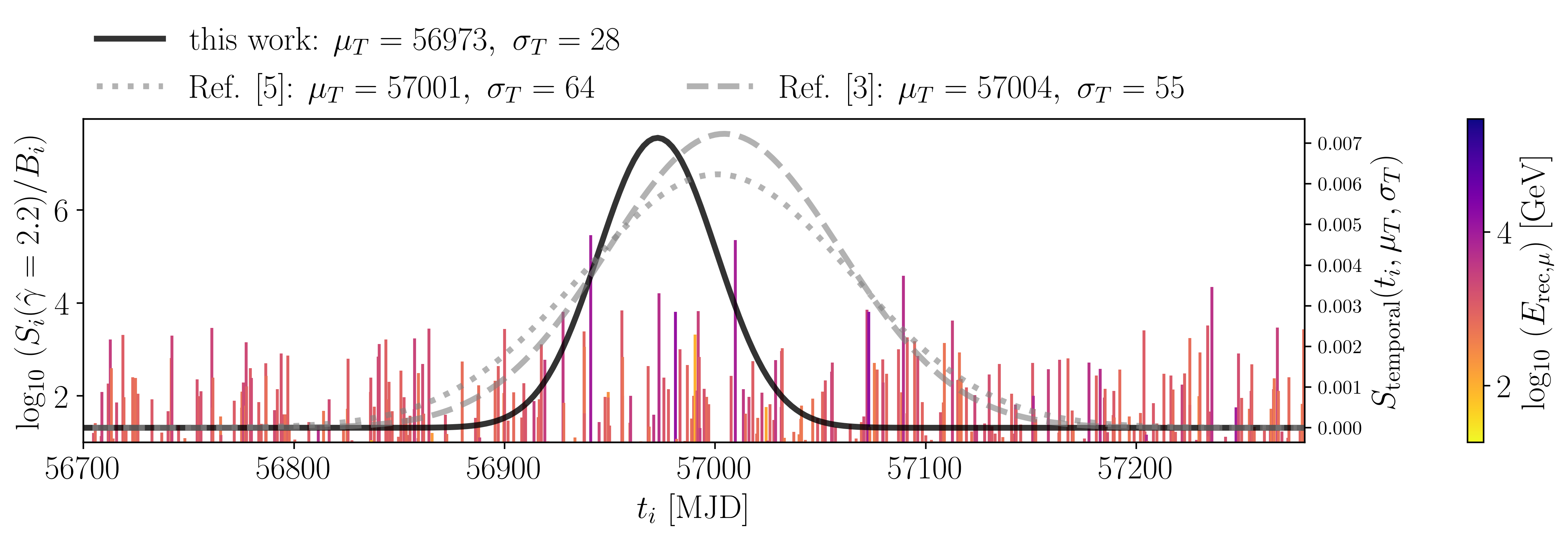
As a final test, we apply EM on IceCube public data at the position of TXS 0506+056 to reproduce the analysis in ref. [3, 4] following the above procedure. Similar to [12], we identify the neutrino flare at a mean time of (MJD) with a width of days. The best-fit parameter of the mean number of neutrinos is and for the spectral index we get . The results are compatible with published IceCube results in [3, 4, 5] (see Figure 5), using more precise energy pdfs based on unpublished Monte Carlo data [12]. This leads to different signal weights for the public data analysis compared to the internal IceCube analyses and influences the flare’s best-fit parameters.
3 Conclusion
We present a new method to fit neutrino flares using Expectation Maximization. We improve the computing time of identifying neutrino flares compared to conventional approaches by (on a single CPU). EM is based on a Gaussian mixture model and can fit different models. It is easily expandable from single to multiple flares and works with multi-dimensional data. We demonstrate the use of EM on a simulated time series of detected neutrino events and, as a last step, demonstrate the application of EM to identify the neutrino flare of TXS 0506+056. The resulting best-fit parameters agree with previously published results.
References
- [1] IceCube collaboration, The IceCube Neutrino Observatory: Instrumentation and Online Systems, JINST 12 (2017) P03012 [1612.05093].
- [2] IceCube, Fermi-LAT, MAGIC, AGILE, ASAS-SN, HAWC, H.E.S.S, INTEGRAL, Kanata, Kiso, Kapteyn, Liverpool telescope, Subaru, Swift/NuSTAR, VERITAS, and VLA/17b-403 collaboration, Multimessenger observations of a flaring blazar coincident with high-energy neutrino IceCube-170922A, Science 361 (2018) eaat1378 [arXiv:1807.08816].
- [3] IceCube collaboration, Neutrino emission from the direction of the blazar TXS 0506+056 prior to the IceCube-170922A alert, Science 361 (2018) 147 [1807.08794].
- [4] IceCube collaboration, Search for Multi-flare Neutrino Emissions in 10 yr of IceCube Data from a Catalog of Sources, The Astrophysical Journal Letters 920 (2021) L45.
- [5] R. Abbasi, M. Ackermann, J. Adams, S.K. Agarwalla, J.A. Aguilar, M. Ahlers et al., Search for continuous and transient neutrino emission associated with icecube’s highest-energy tracks: An 11-year analysis, 2309.12130.
- [6] IceCube collaboration, Searches for time-dependent neutrino sources with icecube data from 2008 to 2012, The Astrophysical Journal 807 (2015) 46.
- [7] IceCube collaboration, A Search for Time-dependent Astrophysical Neutrino Emission with IceCube Data from 2012 to 2017, Astrophys. J. 911 (2021) 67.
- [8] IceCube collaboration, Search for high-energy neutrino sources from the direction of IceCube alert events, in 37th International Cosmic Ray Conference, p. 940, Mar., 2022, DOI [2107.08853].
- [9] M.S. Karl, Unraveling the origin of high-energy neutrino sources: follow-up searches of icecube alert events, 2022.
- [10] IceCube collaboration, Search for neutrino sources from the direction of IceCube alert events, in 39th International Cosmic Ray Conference, vol. ICRC2023, p. 974, 2023.
- [11] IceCube collaboration, IceCube Data for Neutrino Point-Source Searches Years 2008-2018, http://doi.org/DOI:10.21234/sxvs-mt83 (2021) [2101.09836].
- [12] IceCube collaboration, Extending SkyLLH software for neutrino point source analyses with 10 years of IceCube public data, in 39th International Cosmic Ray Conference, vol. ICRC2023, p. 1061, 2023.
- [13] A.P. Dempster, N.M. Laird and D.B. Rubin, Maximum Likelihood from Incomplete Data via the EM Algorithm, Journal of the Royal Statistical Society. Series B (Methodological) 39 (1977) 1.
- [14] W. Press, W. H, S. Teukolsky, W. Vetterling, S. A and B. Flannery, Numerical Recipes 3rd Edition: The Art of Scientific Computing, Cambridge University Press (2007).