Efficient Asynchronous Federated Learning with Sparsification and Quantization

Abstract

[Summary] While data is distributed in multiple edge devices, Federated Learning (FL) is attracting more and more attention to collaboratively train a machine learning model without transferring raw data. FL generally exploits a parameter server and a large number of edge devices during the whole process of the model training, while several devices are selected in each round. However, straggler devices may slow down the training process or even make the system crash during training. Meanwhile, other idle edge devices remain unused. As the bandwidth between the devices and the server is relatively low, the communication of intermediate data becomes a bottleneck. In this paper, we propose Time-Efficient Asynchronous federated learning with Sparsification and Quantization, i.e., TEASQ-Fed. TEASQ-Fed can fully exploit edge devices to asynchronously participate in the training process by actively applying for tasks. We utilize control parameters to choose an appropriate number of parallel edge devices, which simultaneously execute the training tasks. In addition, we introduce a caching mechanism and weighted averaging with respect to model staleness to further improve the accuracy. Furthermore, we propose a sparsification and quantitation approach to compress the intermediate data to accelerate the training. The experimental results reveal that TEASQ-Fed improves the accuracy (up to 16.67% higher) while accelerating the convergence of model training (up to twice faster).

1 Introduction

With more and more data generated and distributed in edge devices (devices), e.g., mobile phones and Internet of Things (IoT) devices, a huge amount of data can be exploited to train a deep learning model for diverse artificial intelligent applications ¹, e.g., image classification ², keyboard prediction ³, location-based social networks^{4, 5}, and etc. Centralized training approaches generally aggregate all the decentralized data to a server or a data center for the training process. These approaches may incur significant huge communication overhead and bring severe privacy security risks ⁶. As an emerging distributed machine learning approach, Federated Learning (FL) ^{7, 8} can enable collaborative training of a machine learning model with distributed raw data while protecting the privacy of the data.

Within the training process of FL, models are updated with the raw data in edge devices and aggregated in a parameter server (server) ⁹. The aggregation of models can be carried out synchronously ^{7, 10} or asynchronously ¹¹. In each round of the whole training process, the server sends the global model to selected devices for local updates before the aggregation of models. The devices update the received model utilizing local data. Then, the devices send back the updated models to the server. With the synchronous method, the server aggregates the updated models to a new global model after receiving the updated models from all the devices. However, devices may have heterogeneous limited computing resources and communication capabilities, e.g., limited computing capabilities, low battery energy, and low bandwidth ¹². As a result, the training process may take a long time, and the communication between devices and the server is inefficient. Furthermore, synchronous aggregation cannot fully exploit the edge devices as the unselected devices remain idle during each global epoch. In addition, some powerful devices need to wait for low devices, i.e., stragglers, to continue following updates. In contrast, with the asynchronous aggregation, the server can update the global model immediately once receiving an updated model from any selected device ¹³, which can take advantage of all the available devices to achieve better performance.

Although asynchronous aggregation can prevent the server from waiting for slow devices, it still suffers from accuracy degradation and inefficient data communication. First, the staleness of the updated models may degrade the accuracy of the global model. For instance, at a given time, the server aggregates the latest models of powerful devices. A show device may just finish the update of a very old global model. Then, the updated model from the slow device may degrade the accuracy of the global model after the aggregation in the server. Second, the issue of non-Independent and Identically Distributed (non-IID) data may also degrade the accuracy of the global model. As the data is generally non-IID, the local optimal model may differ from the global optimal model. The direct aggregation of models from devices may correspond to a global model of inferior accuracy. Finally, as the bandwidth between the devices and the server is limited, it takes much time to transfer the models without sparsification ¹⁴ or quantization ¹⁵.

In this paper, we propose a Time-Efficient Asynchronous FL approach with Sparsification and Quantization (TEASQ-Fed) to improve the training efficiency and the model accuracy of FL. We exploit the idle time of devices more aggressively within the training process. While in the existing schemes devices wait for the task assignment from the server passively, in this work we enable idle devices to apply for training tasks actively. However, in order to reduce the slow convergence brought by large numbers of parallel devices participating in the training process, we propose a control parameter C-fraction. In addition, we utilize a regularization term to improve the stability of the training process with non-IID data. Moreover, to alleviate the staleness issue of asynchronous training, we exploit a caching mechanism and aggregate models with respect to staleness. Finally, we propose a dynamic decaying approach to choose appropriate compression parameters while exploiting sparsification and quantization to reduce the communication cost during the training process. This paper is an extended version of a conference version ¹⁶. The main contributions of this paper are:

1. The design of an asynchronous FL approach, i.e., TEASQ-Fed, to fully exploit devices for the training process. We propose a control parameter to limit the concurrent device participation in order to achieve fast convergence.

2. A model aggregation approach composed of a regularization method and staleness based mechanism to address the problem of non-IID data and the impact of staleness.

3. A dynamic decaying approach to generate appropriate compression parameters while exploiting sparsification and quantization for efficient data transfer between devices and the server (extra contribution compared with ¹⁶).

4. An extensive evaluation, based on Fashion-MNIST and a convolutional neural network with 100 devices, diverse data distributions, and multiple combinations of control parameters of TEASQ-Fed, compared with baseline approaches (with extra extensive experimental results for the sparsification and quantization approach compared with ¹⁶).

The rest of this paper is structured as follows. Section 2 reviews the related work. Section 3 formulates optimization problems of FL. Section 4 provides the detailed explanation of TEASQ-Fed. In Section 5, we conduct extensive experiments with different data sets and data distributions and demonstrate the impact of hyper-parameters. Finally, Section 6 concludes this paper.

2 Related Work

With the wide usage of edge devices, the computation is carried out in edge devices, i.e., edge computing, to deal with the large amounts of data generated and distributed ¹⁷ in edge devices. As an emerging machine learning paradigm, FL is an effective solution to address the communication delay, data scalability, and privacy challenges brought by the centralized training process ^{18, 19}. FL has been widely used in multiple areas with the integration with edge computing, e.g., keyboard prediction ³, edge intelligence ²⁰, and video surveillance ²¹. However, the training process of FL with existing approaches faces two challenges, i.e., accuracy degradation due to non-IID data and low efficiency owing to a huge amount of heterogeneous devices of modest computation and communication capacity.

While the convergency of FedAvg is theoretically analyzed with non-IID data ²², some other methods are proposed to address the accuracy degradation brought by non-IID data within the synchronous model aggregation mechanism. For instance, FedProx ¹² is proposed based on regulization on each device to address the non-IID data issue. A data sharing method ²³ is exploited to improve the accuracy with non-IID data. However, these methods cannot be directly exploited in the asynchronous mechanism.

Existing FL approaches generally exploit a synchronous model aggregation mechanism, which corresponds to inefficient training. FedAvg ⁷ is a representative synchronous model aggregation mechanism, which randomly selects available devices for the training. To deal with the heterogeneity of devices in terms of communication and computing capabilities, diverse device selection methods are proposed ²⁴, e.g., greedy-based ²⁵, Bayesian optimization-based ¹⁰, and reinforcement learning-based ¹⁰. PyrmidFL²⁶ exploits data and system heterogeneity within selected clients, determines the utility-based client selection and then optimizes utility profiling locally. Although these methods can improve the efficiency with proper device selection, the server still needs to wait until the updated model of the slowest selected device is uploaded to the server.

Asynchronous methods ^{13, 27} are proposed to address the straggler issue and improve the utilization of devices. FedBuff²⁸ is an asynchronous federated optimization framework using buffered asynchronous aggregation, where clients conduct local training and communicate with the server asynchronously. The server aggregates multiple client updates in a secure buffer before performing a server update. Based on the notion of concurrency, i.e., the number of workers that compute gradients in parallel, theoretical analysis shows a much faster convergence rate for asynchronous FL ²⁹. However, in these existing asynchronousy FL methods, the devices are passively triggered by the server for model training and some idle devices are not utilized, meanwhile the advanced data compression for transmission is not incorporated. A semi-asynchronous method SAFA is proposed to improve the efficiency of FL ³⁰, which does not consider the non-IID data within diverse devices. Similarly, a layerwise asynchronous model update and temporally weighted aggregation are proposed to improve communication efficiency ³¹, which still corresponds to synchronous communication in terms of the whole model. Asynchronous federated unlearning ³² is also studied in the literature, which divides the clients into clusters (subsets), conducts independent and asynchronous model training for clusters (subsets). The unlearning cost is limited due to the client partitioning. Federated unlearning is out of the scope of this paper.

In order to address the communication bottleneck with FL, diverse techniques ^{33, 34, 35, 36, 37, 38, 39, 40, 41, 42} can be exploited, e.g., sparsification, quantization, and pruning. Model sparsification transfer has been widely exploited in distributed machine learning ^{43, 15, 44, 14, 45}. A typical sparsification method is the Top-K sparsification ¹⁴, where the K largest values in the tensor are selected and retained, and the rest of the values are set to zero so that the sparse tensor will be easier to compress and transmit in practical application scenarios. Model quantization is also utilized in distributed machine learning as well as FL. Quantization is the process of compressing the representation of values with a smaller number of bits to reduce the size of the values ¹⁵. The reset transmission error method is proposed to remend the global model by adjusting the errors brought by the quantization or sparsification ⁴⁴. However, this method incurs extra synchronizations and leads to significant communication overhead. In addition, model pruning techniques ^{46, 47, 48} can be exploited to reduce the huge overhead of computation and communication during the whole training process. In FedCG⁴⁹, the server selects a representative client subset for local training considering statistical heterogeneity and then these selected clients upload compressed model updates matching their capabilities for aggregation, which alleviates the communication load and mitigates the straggler effect. FedLamp ⁵⁰ adaptively determines diverse and appropriate local updating frequencies and model compression ratios in the resource-constrained edge computing systems, so as to reduce the waiting time and enhance the training efficiency. However, these above approaches cannot choose the appropriate parameters for the data compression of both sparsification and quantization with accuracy degradation constraints, which may lead to unexpected accuracy degradation.

In this paper, we propose a new time-efficient approach to efficiently exploit devices to train a global model in FL while addressing the problem brought by non-IID data. In addition, we exploit sparsification and quantization with proper data compression parameters to improve communication efficiency while satisfying the accuracy degradation constraints.

3 Problem Formulation

Table 1: Summary of Main Notations

Notation	Definition
$N$; $k$	The number of devices; the index of devices
$\mathcal{D}_{k}$; $n_{k}$	Local dataset on device $k$; size of samples
$w^{g}$; $S_{w^{g}}$	The global weight; size of the global weight
$w^{l}$; $S_{w^{l}}$	The local weight; size of the local weight
$p_{s}$; $p_{q}$	Sparsification parameter; quantization parameter
$r^{d}_{k}$	The maximum transmission rate of downloading global models for device $k$
$r^{u}_{k}$	The maximum transmission rate of uploading local models for device $k$
$S_{w^{g},p_{s},p_{q}}$	The size of compressed global model weights
$S_{w^{l},p_{s},p_{q}}$	The size of compressed local model weights
$L^{down}_{k,t}$	The latency of downloading global model weights
$L^{up}_{k,t}$	The latency of uploading global model weights
$L^{cp}_{k,t}$	The latency of model computation
$L^{round}_{k,t}$	The total time of round $t$ for device $k$
$L_{T}$	The total time for $T$ rounds of asynchronous FL
$Set_{p}$	The set of candidate parameter $p_{s}$
$Set_{q}$	The set of an available number of bits in the quantization process $p_{q}$

In this section, we formulate the problem to address in this paper. We first present the overview of an FL system. Then, we present the latency model. Finally, we present the problem statement. The summary of the main notations is shown in Table 1.

We consider an FL system consisting of a server module (server) and N devices. We consider idle time as the time slot when a device has no task to execute. Once receiving an updated model from a device, the server aggregates the global model with the updated model. $n_{k}$ samples are stored on the $k$-th device where $k\in\{1,...,N\}$. The total number of samples can be calculated as $n=\sum_{k=1}^{N}n_{k}$. The training objective is to update the global model with the weight parameters $w$ utilizing the local data of all edge devices, which is formulated as follows:

$$\min_{w\in\mathbb{R}^{d}}f(w)=\sum_{k=1}^{N}\frac{n_{k}}{n}{\rm E}_{x_{k}\sim\mathcal{D}_{k}}[f_{k}(w;x_{k})]$$ (1)

where $x_{k}$ is sampled from the local dataset $\mathcal{D}_{k}$ on device $k$, and $n_{k}=|\mathcal{D}_{k}|$. $f_{k}(w;x_{k})=l(w;x_{k})$ is the loss calculated on device $k$ with the sample $x_{k}$ and the parameters $w$. We assume that the data distributions on devices are not Identically Independently Distributed, i.e., non-IID.

3.1 Latency Model

In this section, we present the model to calculate the latency for the training process, including communication latency, computation latency, and round latency.

3.1.1 Communication Latency

When the server and devices communicate with each other, either the server sends the global model to the devices or the devices upload updated local models to the server. We denote the global model weight as $w^{g}$, which consists of values in float32 without quantization, and we denote the size of $w^{g}$ as $S_{w^{g}}$ in bits. Similarly, the size of local model weight $w^{l}$ is denoted as $S_{w^{l}}$ in bits. When exploiting sparsification and quantization with the corresponding parameters of $p_{s}$ and $p_{q}$, respectively, the size of local model weight becomes $S_{w^{l},p_{s},p_{q}}$. $p_{s}$ represents the ratio of the non-zero values kept in the model within the sparsification process and $p_{q}$ corresponds to the number of bits, e.g., float32 or int8, to represent each value within the quantization process. The maximum transmission rate of the $k$-th device (bits/s), where $k\in\{1,...,N\}$, for the server to send global models is defined as $r^{d}_{k}$. Similarly, the maximum transmission rate of devices uploading local models (bits/s) is defined as $r^{u}_{k},\forall k\in\{1,...,N\}$. We assume that $r^{u}_{k}$ and $r^{d}_{k}$ remain constant during training. Thus, for each device $k\in\{1,...,N\}$ and each round $t\in\{1,...,T\}$, the global model download latency is $L^{down}_{k,t}=\frac{S_{w^{g},p_{s},p_{q}}}{r^{d}_{k}}$, and the local model upload latency is $L^{up}_{k,t}=\frac{S_{w^{l},p_{s},p_{q}}}{r^{u}_{k}}$.

3.1.2 Computation Latency

To characterize the randomness of the computation latency of local model update, we exploit the shifted exponential distribution ⁵¹:

$$\mathbb{P}[L^{cp}_{k,t}<l]=\begin{cases}1-e^{-\frac{\phi_{k}}{\tau b}(l-a_{k}\tau b)},&l\geq a_{k}\tau b,\\ 0,&\rm{otherwise},\end{cases}$$ (2)

where $a_{k}>0$ represents the maximum of computation capabilities, and $\phi_{k}>0$ represents the fluctuation of computation capabilities. We assume that $a_{k}$ and $\phi_{k}$ remain constant during training. The computational delay of device $k$ in round $t$ is denoted as $L^{cp}_{k,t}$. The latency of model computation (i.e., $L^{cp}_{k,t}$) can also be affected by the time to compress the local model and the time to decompress the global model, but since these two components of latency are usually much smaller than the time to update the model, they are ignored in this paper.

3.1.3 Round Latency

For a certain round $t$, and a certain device $k$, the total time of a round, i.e., the time period between the downloading of the global model to the uploading of the trained local model, is defined as:

$$L^{round}_{k,t}=L^{down}_{k,t}+L^{cp}_{k,t}+L^{up}_{k,t},$$ (3)

when device $k$ uploads its updated local mode to the server in round $t$.

We define the total time for $T$ rounds of asynchronous FL as $L_{T}$. However, due to the asynchronous nature among multiple rounds, we cannot simply sum them up to obtain the total time consumed by the $T$-round asynchronous FL. In addition, because of asynchronicity, we cannot intuitively describe the relationship between $L_{T}$ and $L^{round}_{k,t},\forall{t\in\{1,...T\}}$ in numerical terms. $L_{T}$ depends on $L^{round}_{k,t},\forall{t\in\{1,...T\}}$, and a smaller $L^{down}_{k,t}$, $L^{cp}_{k,t}$, or $L^{up}_{k,t}$ can reduce $L_{T}$ in the asynchronous FL system. Then, we describe the relationship by a function $g(\cdot)$:

$$L_{T}=g(L^{round}_{k_{1},1},L^{round}_{k_{2},2},...,L^{round}_{k_{T},T}),$$ (4)

where $k_{t}\in\{1,2,...,N\}$ represents the device for round $t$, i.e., each round is indicated by the update of device $k_{t}$. $g(\cdot)$ represents the total time of the whole asynchronous FL process.

3.2 Problem Statement

We formulate the overall optimization objective as follows:

$$\min_{w}f(w) =\sum\nolimits_{k=1}^{N}\frac{n_{k}}{n}{\rm E}_{x_{k}\sim\mathcal{D}_{k}}[f_{k}(w,p_{s},p_{q};x_{k})]$$

$$s.t.\qquad g(p_{s},p_{q};L^{round}_{k_{1},1},L^{round}_{k_{2},2},...,L^{round}_{k_{T},T})\leq L,$$

$$k\in\{1,...N\},$$

$$t\in\{1,...T\},$$

$$p_{s}\in Set_{p},$$

$$p_{q}\in Set_{q},$$

$$w\in\mathbb{R}^{d}$$

where $x_{k}$, $n_{k}=|\mathcal{D}_{k}|$, $f_{k}(\cdot)$ are the same as those in Formula (1). $L$ is the total time budget and $g(\cdot)$ is the estimated training time. $p_{s}$ is the parameter for sparsification and $p_{q}$ is the parameter for quantization. $Set_{p}$ represents the set of candidate parameters $p_{s}$, $Set_{q}$ represents the set of an available number of bits in the quantization process.

4 TEASQ-Fed Protocol

We propose a new asynchronous FL approach, i.e., TEASQ-Fed, to collaboratively train a model. TEASQ-Fed consists of four parts. First, we asynchronously exploit the edge devices in the training process of FL. Second, we utilize a regularization method to address the problem of non-IID data and the impact of staleness. Third, we generate appropriate compression parameters while exploiting sparsification and quantization. In this section, we present the details of TEASQ-Fed, including the protocol overview, task management, model aggregation, sparsification, and quantization.

4.1 Asynchronous Protocol Overview

Figure 1: The overview of TEASQ-Fed protocol.

Diverse devices are exploited based on their private local data in the training process of FL, while the data distribution is generally heterogeneous, i.e., non-IID. Moreover, in the synchronous training method (e.g., FedAvg ⁷), the selected devices may be busy or crash while performing training tasks, which may prolong the training process. On the contrary, in our proposed asynchronous protocol edge devices initiate training task requests proactively when they are idle, which can alleviate the device unavailability issue during training. Besides, we propose a cache mechanism and a weighted averaging method with regularization for the server to increase the convergence speed of the model training.

The overview of TEASQ-Fed protocol is shown in Figure 1. At the beginning, the server initializes a global model randomly. The idle edge device sends a request to the server to obtain a training task (Step \footnotesize1⃝ in Figure 1). After receiving the task request from the device, the server checks whether the number of devices currently participating in the latest model training is less than a limit. If the limit is not reached, the latest global model is delivered to the device and change the record of the number of devices participating in training the latest global model, otherwise it is not delivered (Step \footnotesize2⃝). The idle devices receiving the global model update the global model asynchronously using their local data and upload the updated model parameters to the server (Step \footnotesize3⃝). The server puts the updated model and time stamp received from devices into the cache, and change the record of the number of these devices participating in training in the same stamp (Step \footnotesize4⃝). The server uses weighted averaging according to staleness to update the global model after it receives updates from a certain number of devices, and then enters the next round of global training (Step \footnotesize5⃝). All steps \footnotesize1⃝ - \footnotesize5⃝ are iterated until the global model achieves the desired performance.

The detailed design of TEASQ-Fed protocol is explained in the following subsections. In Subsection 4.2 and 4.3, we describe the training task request and local model update (Algorithm 1). Idle devices request training tasks from the server proactively. When the number of parallel devices participating in the training process is significant, the final convergence may degrade due to the diverse version of the original model. Thus, we set a limit on the number of parallel training devices when distributing training tasks. In Subsection 4.4, we describe the global model update on the server (Algorithm 2). We adopt a caching mechanism with a weighted average mechanism for model aggregation to further improve the accuracy. In Subsection 4.5, we describe the dynamic weight compression method with sparsification and quantization as well as compression parameter selection (Algorithm 3, 4 and 5).

Algorithm 1 Training task request and local model training.

$N$: the quantity of edge devices

$T$: the quantity of rounds

$E$: the quantity of local updates per round

$B$: minibatch size of local updates

$\eta$: learning rate

$\mu$: the weight of regularization

$P$: the quantity of edge devices taking part in training during the $t$-th training round

$C\in\left(0,1\right)$: the proportion of edge devices

Server process:        // on the server
Initialize $w^{0}$, $t\leftarrow 0$, $P\leftarrow 0$
Distributor:

1:Receive request from the inactive edge device

2:if $P\leq[N\cdot C]$ then        //$P$ represents the number of selected devices

3:     Compress the latest model $w^{t}_{compress}=\mathcal{C}(w^{t},p_{s},p_{q})$

4:     Transfer the latest compressed model $w^{t}_{compress}$ to the requested device

5:     Update $P\leftarrow P+1$

6:end if

Device process:        // on inactive device $k$

1:if device $k\in\left[N\right]$ is idle then

2:     Send training task request to the server

3:     if receive $\left(w^{t}_{compress},t\right)$ from the server then

4:         Decompress $w^{t}=\mathcal{C}^{-1}(w^{t}_{compress})$

5:         $\chi_{k}\leftarrow$ (split $\mathcal{D}_{k}$ into batches of size $B$)

6:         $w^{h_{k}}_{k}\leftarrow w^{t}$

7:         for each local epoch $i$ from 1 to $E$ do

8:              for batch $x_{k}\in\chi_{k}$ do

9:                  $w^{h}_{k}=w^{h}_{k}-\eta\left(\nabla f_{k}(w^{h}_{k};x_{k})+\mu(w^{h}_{k}-w^{t})\right)$

10:              end for

11:         end for

12:         Compress the updated local model $w^{h}_{compress,k}=\mathcal{C}(w^{h}_{k},p_{s},p_{q})$

13:         Transfer the updated local model and time stamp $(w^{h}_{compress,k},h)$ to the server

14:     end if

15:end if

4.2 Task Management

Algorithm 2 Model aggregation.

$N$: the quantity of edge devices

$T$: the quantity of rounds

$\gamma\in\left(0,1\right)$: cache fraction

$\alpha\in\left(0,1\right]$: the hyper-parameter for aggregation

Server process:    // performing on the server
Receiver:

1:Get an update $w^{h_{c}}_{compress,k_{c}}$ and the time stamp $h_{c}$ from any inactive device

2:Push $\left(w^{h_{c}}_{compress,k_{c}}\right)$ into the cache queue $Q$

3:Update $P\leftarrow P-1$

Updater:

1:for round $t=0,1,...,T-1$ do

2:     for $c=1$ to $\left[N\cdot\gamma\right]$ do

3:         Pop $\left(w^{h_{c}}_{compress,k_{c}}\right)$ from the cache queue $Q$

4:         Decompress $w^{h_{c}}_{k_{c}}=\mathcal{C}^{-1}(w^{h_{c}}_{compress,k_{c}})$

5:     end for

6:     Calculate the aggregated model weight according to Formula (7) and (8)

7:     Calculate the global model $w^{t+1}$ according to Formula (9) and (10)

8:end for

With existing FL systems ^{7, 25}, the devices are generally randomly selected by the server in each round. Insufficient battery power, unstable network conditions, and device crashes may affect the training of some devices, making them unreliable. Moreover, after completing the training task, the selected device may remain idle. The device will not be selected again until the next round of training. Furthermore, idle devices other than the selected one are not fully utilized. As a strategy for improving the utilization of devices, we exploit asynchronous communication to enable idle devices to actively participate in training tasks. Thus, if the device is assigned a training task, it sends a task request to the server once it becomes idle, and the server sends the latest model to it.

As large amounts of device participation within the FL training process may incur slow convergence, The hyper-parameter $C$ controls how many devices participate in the parallel training from the same global model. By implementing the $C$-fraction, the model ²² can be guaranteed to have a speedy convergence and prevent server overload due to excessive participants. Algorithm 1 indicates that when a task request comes from a device that is idle, the server determines whether to immediately serve the latest model (Line 2). Devices taking part in the latest model training will receive the latest model only if the number is less than $\left[N\cdot C\right]$; otherwise, it will not. A model received from the server will then be updated by the idle device with local data once it receives a model from the server. The TEASQ-Fed suffers from a slow convergence speed, if $C$ is set too small. A large $C$ will increase the risk of congestion and also slow down the convergence speed. It is true that the idle devices may introduce biases; however, we believe that these biases are negligible since our approach provides a much higher degree of accuracy than FedAvg (see details in Section 5.2).

As shown in Algorightm 3, $\mathcal{C}(w,p_{s},p_{q})$ compresses all the tensors in model $w$ to get compressed model weights $w_{compressed}$, i.e., $w_{compressed}$ = $\mathcal{C}(w,p_{s},p_{q})$. The sparsification ¹⁴ operation is explained in Lines 4-5. The quantization ⁵² operation is explained in Line 6. We remove these zero elements in Line 7.

4.3 Local Update

Since diverse devices store data in non-IID manners ¹², the local updates of some devices may slow down the global model convergence speed. We exploit a penalty term based on ^{12, 13} to reduce adverse impacts of the non-IID data. The loss function in an idle device $k$ contains a regularization term with the global model $w$ received from the server as defined:

$$\min\limits_{w\in\mathbb{R}^{d}}{\rm E}_{x_{k}\sim\mathcal{D}_{k}}[f_{k}(w;x_{k})]+\frac{\mu}{2}\parallel w-w^{t}\parallel^{2}$$ (5)

Regularization weights are parameterized as $\mu$. Using the penalty term can reduce data heterogeneity and make the model more stable.

4.4 Model Aggregation

The server and idle devices are updated asynchronously during model training, as shown in Algorithm 2. The server puts the received updates into the cache and utilizes them for aggregation later. With the help of the hyper-parameter $\gamma$, we limit the size of the cache or the total number of uploaded updates in the cache. We first execute elastic averaging between the most recent local averaging update and the current global model, which not only utilizes the knowledge of new updates but also does weighted averaging on the cached updates. The global model can converge quickly and smoothly in this way.

4.4.1 Update Caching Mechanism

In the existing asynchronous methods ¹³, the server immediately updates the global model upon receiving a local update from any device and then moves on to the subsequent training phase. Although this mechanism results in a significant throughput, a single poor local update could lead to a divergence in the global model. We exploit a caching mechanism to reduce the negative effects of model staleness and increase the stableness of the global model. We set the cache capacity to the size of $K=\left[N\cdot\gamma\right]$ local updates, where $\gamma\in\left(0,1\right)$. We denote the cached updates as $\mathcal{U}=\left\{\left(k_{c},w_{k_{c}}^{h_{c}}\right)\right\}_{c\in[0,K]}$, where $w_{k_{c}}^{h_{c}}$ is the $c$-th update in the cache from device $k_{c}$ with time stamp of global model $h_{c}$. After receiving $K$ local updates, the server changes the global model through weighted averaging depending on the staleness of each update. In the paper, we set the value of $\gamma$ to 0.1.

Algorithm 3 Compress the model weight tensor.

1:$p_{s}$, $p_{q}$, Uncompressed model weight $w$

2:Compressed model weight $w_{compressed}$

3:for $tensor\in w$ do

4:     $values$ $\leftarrow$ Top $p_{s}\%$ elements of $tensor$

5:     Elements of $tensor$ not in $values$ are set to 0

6:     Quantize $tensor$ to $p_{q}$ bits

7:     $values,indices\leftarrow$ non-zero elements in $tensor$

8:     $tensor\leftarrow concat(values,indices)$

9:end for

10:Combine $tensor$ to $w_{compressed}$ and return

Algorithm 4 Decompress the model weight tensor.

1:Compressed model weight $w_{compressed}$

2:Decompressed model weight $w_{decompressed}$

3:for $tensor_{compressed}\in w_{compressed}$ do

4:     $values,indices$ = $tensor_{compressed}$

5:     Restore $tensor$ with $values$ and $indices$

6:     Cast $tensor$ to $32$-bits (float32)

7:end for

8:Combine $tensor$ to $w_{decompressed}$ and return

Algorithm 5 Dynamic data compression.

$w$: pre-trained model weight

$\theta$: the predefined threshold

$Set_{s}$: the set of sparsification parameters

$Set_{q}$: the set of quantization parameters

$T$: the maximum number of rounds

$p_{s,t}$ and $p_{q,t}$ $\forall t\in\{1,2,...,T\}$

1:$acc\leftarrow test(w)$

2:$p_{s}$ $\leftarrow$ $p_{s}^{\prime}\in Set_{s}$ with the smallest compression rate

3:$p_{q}$ $\leftarrow$ 0$\triangleright$ No quantization

4:while $test(\mathcal{C}^{-1}(\mathcal{C}(w,p_{s},p_{q})))\geq acc$ - $\theta$ and the compression rate can be reduced do

5:     while $test(\mathcal{C}^{-1}(\mathcal{C}(w,p_{s})))$ $\geq$ $acc$ - $\theta$ do

6:         $p_{s}$ $\leftarrow$ $p_{s}^{\prime}\in Set_{s}$ with a bigger compression rate

7:     end while

8:     $p_{q}$ $\leftarrow$ $p_{q}^{\prime}\in Set_{q}$ with a bigger compression rate

9:     while  $test(\mathcal{C}^{-1}(\mathcal{C}(w,p_{s},p_{q})))$ $\leq$ $acc$ - $\theta$  do

10:         $p_{s}$ $\leftarrow$ $p_{s}^{\prime}\in Set_{s}$ with a smaller compression rate

11:     end while

12:end while

13:$p_{s,0}$ $\leftarrow$ the element in $Set_{s}$ corresponding to a bigger compression rate than that of $p_{s}$

14:$p_{q,0}$ $\leftarrow$ the element in $Set_{q}$ corresponding to a bigger compression rate than that of $p_{q}$

15:for $t\in[T]$  do

16:     $p_{s,t}\leftarrow$ $p_{s,0}$ decay $\lfloor\frac{t}{step\_size}\rfloor$ steps

17:     $p_{q,t}\leftarrow$ $p_{q,0}$ decay $\lfloor\frac{t}{step\_size}\rfloor$ steps

18:end for

19:Return $p_{s,t}$ and $p_{q,t}$ $\forall t\in[T]$

4.4.2 Staleness-Based Weighted Averaging

The staleness of local updates in the cache may differ as the models in devices and the server are updated asynchronously. We denote the latest global model in round $t$ on server as $w^{t}$. Then the staleness of the $c$-th update in the cache $w_{k_{c}}^{h_{c}}$ is $t-h_{c}$. We define a function $S(\cdot)$ with respect to the staleness as follows:

$$S\left(t-h_{c}\right)=\left(t-h_{c}+1\right)^{-a},a>0,$$ (6)

where $a$ is a hyper-parameter. After the server caches $K=\left[N\cdot\gamma\right]$ updates, the average update $u$ can be calculated as follows:

$$u=\frac{\sum\nolimits_{c=1}^{K}S\left(t-h_{c}\right)\frac{n_{k_{c}}}{n}w^{h_{c}}_{k_{c}}}{\sum\nolimits_{c=1}^{K}S\left(t-h_{c}\right)\frac{n_{k_{c}}}{n}}=\frac{\sum\nolimits_{c=1}^{K}S\left(t-h_{c}\right)n_{c}w^{h_{c}}_{k_{c}}}{\sum\nolimits_{c=1}^{K}S\left(t-h_{c}\right)n_{k_{c}}},$$ (7)

We use $\delta$ to represent the average staleness of all local weights in the cache,

$$\delta=\frac{1}{K}{\sum\nolimits_{c=1}^{K}(t-h_{c})}.$$ (8)

With Formulas (6) and (7), the value of mixing weight $\alpha^{t}$ in the $t$-th round is calculate by

$$\alpha^{t}=\alpha\cdot S\left(\delta\right),$$ (9)

where $\alpha\in\left(0,1\right]$ is the mixing hyper-parameter. Finally, the server updates the global model $w^{t}$ with weighted averaging to calculate a new global model $w^{t+1}$ according to

$$w^{t+1}=\alpha^{t}u+\left(1-\alpha^{t}\right)w^{t}.$$ (10)

4.5 Dynamic Weight Compression

In order to improve the communication efficiency within the FL training process, we exploit sparsification ¹⁵ and quantization ⁵² to compress the model. Sparsification compresses a model taking a subset of the original model parameters to represent the original model, e.g., Random-K ¹⁴ and Top-K ¹⁵. Quantization reduces the number of bits in each element of the model parameters from the original 32-bit floating point number to a smaller number of bits, e.g., 8-bit. We can exploit existing sparsification ^{14, 15} and quantization ^{52, 45} compression mechanisms to compress the model.

In Algorithm 1, $\mathcal{C}(w,p_{s},p_{q})$ represents the data compression with two steps, i.e., sparsification with parameter $p_{s}$, and quantization with parameter $p_{q}$. The decompression operation (i.e., $\mathcal{C}^{-1}(w)$) is the inverse process of the above two steps. The compression method $\mathcal{C}(w,p_{s},p_{q})$ adapts the Top-K method ¹⁵ and the QSGD method ⁴⁵ as shown in Algorithm 3. The decompression of weights (i.e., $\mathcal{C}^{-1}(w)$) is presented in Algorithm 4. First, the values and indices are retrieved from the tensor in Line 4. Then, the original shape of the tensor is restored in Line 5. Finally, the type of the tensor is converted back to float32 in Line 6.

Figure 2: Impacts of $\mu$ in terms of accuracy vs. training time with non-IID dataset.

With inappropriate values of $p_{s}$ or $p_{q}$, the accuracy may be significantly reduced and the data communication efficiency remains low. As shown in Algorithm 5, we propose a heuristic method, i.e., dynamic data compression, to generate proper values as $p_{s}$ and $p_{q}$ with a decay mechanism. We propose a greedy method to calculate appropriate values for $p_{s}$ and $p_{q}$. In order to analyze the impact of the values of $p_{s}$ and $p_{q}$ on the accuracy, we take a trained model $w$ to profile the accuracy with diverse values of $p_{s}$ and $p_{q}$. First, in Lines 5-7, we choose the highest compression rate of $p_{s}$ without quantization. Then, we take a value of $p_{q}$ that corresponds to a higher compression rate of quantization in Line 8 and decrease the compression rate of $p_{s}$ in Lines 5-7 until the accuracy degradation satisfies a predefined threshold. Afterward, we repeat the aforementioned step of adjustment of $p_{s}$ in Lines 4-12. If the compression can be further reduced, we continue. Otherwise, we finish the search process. In addition, in order to achieve high accuracy with sparsification and quantization, we propose a dynamic method by decaying the compression ratio during the training process in Lines 13-18. $\mathcal{C}(w,p_{s})$ in Line 5 represents compressing $w$ with only the sparsification method, and $\mathcal{C}(w,p_{s},p_{q})$ in Line 9 represents compressing $w$ with both sparsifaication and quantization methods. Lines 13-18 represent compression parameter decay process. Based on the $p_{s}$ and $p_{q}$ searched, we start with a relatively low compression rate (i.e., $p_{s,0}$ and $p_{q,0}$) and increase the compression rate using a constant step size. After determining the compression parameters for each round, the server and each device will compress and decompress model weights in round $t$ using $p_{s,t}$ and $p_{q,t}$.

5 Experimental Evaluation

We carry out extensive experimentation to evaluate TEASQ-Fed. To demonstrate the efficacy of TEASQ-Fed, we measure the convergence with various machine learning tasks and data distributions.

5.1 Experiment Setup

Table 2: The summary of the Fashion-MNIST dataset.

Image scale	28 $\times$ 28
Image type	grayscale
# training samples	60,000
# testing samples	10,000
# categories	10

To evaluate the performance of TEASQ-Fed, we carry out extensive experimentation on the Fashion-MNIST dataset ⁵³. As shown in Table 2, this dataset includes 70,000 grayscale photos in total, with 60,000 training images and 10,000 testing images, of diverse products from 10 categories. We exploit the dataset to conduct picture categorization with a convolutional neural network (CNN). The CNN consists of two $2\times 2$ convolutional layers, a fully connected layer, and a softmax output. We assume that the resource-constrained edge devices are capable of training this lightweight CNN network.

We uniformly distribute the training data among 100 edge devices. We employ an experimental set-up that is similar to the existing work ²³ in order to evaluate the performance of TEASQ-Fed under various data distributions. Each device randomly selects a predetermined number of photos from each training batch for the IID setting. The training data is sorted into classes based on categories for non-IID settings. Then, a subset of 2 classes is chosen at random from a total of 10 classes, and each device randomly samples images from this subset. We set $a$ = 0.5 in Formula (6) ¹³ and $\gamma$ = 0.1 in each cycle of the TEASQ-Fed protocol.

((a)) Non-IID

((b)) IID

Figure 3: Impacts of $C$ in terms of accuracy vs. training time with non-IID and IID dataset.

We take FedAvg ⁷ and FedASync ¹³ as synchronous and asynchronous FL baselines. In the experiment, the maximum model staleness is maintained at 4 for FedASync, and 10 devices are randomly chosen for FedAvg in each cycle to carry out the local update. Additionally, we used the TEAStatic-Fed approach, in which the compression parameters are maintained constant during the training phase, to confirm the impact of dynamic parameter decay. We refer to TEASQ-Fed without sparsification or quantization by TEA-Fed in this part.

To verify the improvement of TEASQ-Fed in the wireless network environment relative to the baselines, we simulate a wireless IoT FL system with a Base Station (BS), i.e., server, and $M$ devices distributed in a circular area. The radius of the circular area is $R=600$ m or $1000$ m. The server is located at the center of the circular area. All devices are uniformly distributed in the circular area whose locations stay unchanged during the whole training process. The wireless bandwidth is $B=20$ MHz. The path loss exponent is $\alpha=3.76$. The transmission power of the BS, i.e., server, is $P_{0}=20$ dBm, and the transmit power of all devices is $P_{k}=10$ dBm. The power spectrum density of the additive Gaussian noise is $N_{0}$ = -114 dBm/MHz. Thus the maximum achievable transmission rate (bits/s) of BS sending global models can be written as $r^{d}_{k}=B\log_{2}(1+\frac{P_{0}h^{2}_{0,k}}{BN_{0}})$ and the maximum achievable transmission rate (bits/s) of devices uploading local models can be written as $r^{u}_{k}=B\log_{2}(1+\frac{P_{k}h^{2}_{k,0}}{BN_{0}})$, where $h_{i,j}$ represents the corresponding channel gain and “0” represents the BS ⁵¹.

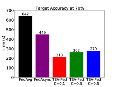
((a)) Non-IID

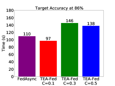
((b)) IID

Figure 4: Impacts of $C$ and time required to reach the target test accuracy with non-IID and IID dataset. In (b), FedAvg fails to reach the target accuracy.

5.2 Evaluation Results

We carry out tests on a variety of hyper-parameters, such as $C$, $\alpha$, and $\mu$, and we examine how these hyper-parameters affect the convergence of the global model. In the meantime, we evaluate the model precision and convergence rates of several optimization strategies for various data distributions.

5.2.1 Effects of $\boldsymbol{\mu}$

We demonstrate the impact of various $\mu$ values on TEASQ-Fed without data compression (i.e., TEA-Fed) using non-IID data in Figure 2. The regularization weight parameter in the local optimization is non-negative, i.e., $\mu\geq 0$. The weights of local updates with the same number of local epochs vary significantly because of the imbalanced data distribution²³. By exploiting a regularization penalty term, the local update limits the local update to be closer to the global model and allows the global model to converge more rapidly and smoothly ¹². We provide a finite set of values for $\mu$, which are $\left\{0,0.001,0.005,0.01,0.1\right\}$. The experimental findings demonstrate that the convergence efficiency of the proposed algorithm with heterogeneous data can be significantly increased when $\mu>0$. The corresponding accuracy, stability with non-IID data, and convergence speed of the global model can all be improved with appropriate $\mu$.

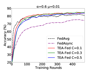
((a)) Non-IID

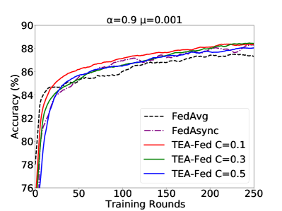
((b)) IID

Figure 5: Impacts of $C$ in terms of accuracy vs. training rounds with non-IID and IID dataset.

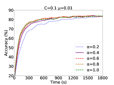
((a)) Non-IID

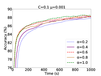
((b)) IID

Figure 6: Impacts of $\alpha$ in terms of accuracy vs. training time with non-IID and IID dataset.

5.2.2 Effects of $\boldsymbol{C}$

We demonstrate how TEASQ-Fed without data compression (i.e., TEA-Fed) converges with various $C$ values over time under non-IID and IID data distributions in Figures 3(a) and 3(b). The results show that the model accuracy and convergence speed of TEA-Fed are not directly proportional to the value of $C$. Although increasing $C$ enhances the parallelism, too many devices are involved in the training process of the same epoch simultaneously, which could result in a significant delay. As a result, the performance rate is the highest when $C$ is 0.1, and TEA-Fed has a higher convergence efficiency than FedAvg and FedAsync. In addition, as depicted in Figures 4(a) and  4(b), TEA-Fed corresponds to a shorter time to obtain the desired precision. The training time required for each round is shorter than the baselines because it effectively decreases the waiting time. We show the convergence of TEA-Fed in terms of training rounds in Figure 5. Evidently, the accuracy of TEA-Fed is significantly higher than that of baselines, further demonstrating its effectiveness under non-IID and IID data distributions.

5.2.3 Effects of $\boldsymbol{\alpha}$

The old global model and the new updated local models are aggregated with the hyper-parameter $\alpha$. The influence of the new update on the updated global model increases with the larger value of $\alpha$. Figure 6 illustrates how TEA-Fed varies with various $\alpha$. As the influence of $\alpha$ between 0.4 and 0.9 on the convergence has little difference, the convergence of TEA-Fed does not depend on $\alpha$. Thus, $\alpha$ has limited influence on the convergence of TEA-Fed, which means TEA-Fed is robust to the change of $\alpha$.

((a)) Non-IID

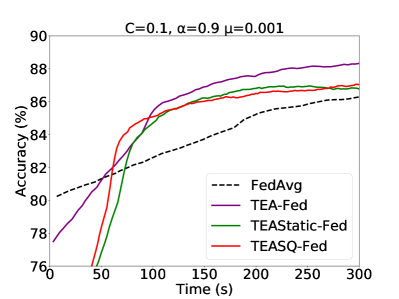
((b)) IID

Figure 7: Impacts of compression in terms of accuracy vs. training time with non-IID and IID dataset.

Table 3: The highest test accuracy within a given time budget using IID data.

	50s	60s	70s	80s	90s	100s	200s	300s
FedAvg (IID)	81.11%	81.29%	81.46%	81.81%	81.98%	82.33%	85.12%	86.34%
TEA-Fed (IID)	80.79%	81.34%	82.16%	82.99%	83.81%	85.23%	87.64%	88.32%
TEAStatic-Fed (IID)	75.79%	77.84%	79.88%	83.45%	84.29%	84.73%	86.82%	86.96%
TEASQ-Fed (IID)	77.37%	80.75%	83.96%	84.65%	84.96%	85.08%	86.47%	87.09%

5.2.4 Effects of Compression

TEASQ-Fed exploits the compression parameters generated from the dynamic decay of $p_{s}$ and $p_{q}$ as shown in Algorithm 5. TEAStatic-Fed represents utilizing the parameters generated from Lines 4-12 in Algorithm 5, where $p_{s}$ and $p_{q}$ are constant during the training process. In Figure 7(a) and Figure 7(b), we compare the accuracy corresponding to TEAStatic-Fed, TEASQ-Fed, and FedAvg with IID (Tables 3, 4) and non-IID (Tables 5, 6) data, respectively. We can see that both TEAStatic-Fed and TEASQ-Fed have a faster convergence speed than FedAvg. TEA-Fed achieves a higher accuracy (up to 16.67% as shown in Figure 5(a)) than FedAvg and converges faster (up to twice faster as shown in Figure 4(a) when target accuracy at 70%) than FedAvg. However, compared to TEA-Fed, due to the lossy data compression of data compression, the training of TEAStatic-Fed and TEASQ-Fed is more efficient at the early stage, while TEAStatic-Fed and TEASQ-Fed cannot converge to the same accuracy as TEA-Fed. When we can have a tight training time for a modest accuracy requirement, dynamic data compression (TEASQ-Fed) can achieve a higher accuracy (up to 10.08% compared with TEA-Fed and up to 32.40% compared with FedAvg as shown in Table 5) within a short training time (100s) or a shorter training time (up to 45.73% compared with TEA-Fed and twice faster compared with FedAvg as shown in Table 6) with a modest target accuracy (68%). In addition, the required storage space corresponding to the dynamic data compression with sparsification and quantization is 44.07% (when uploading local models) smaller than that of FedAvg, as shown in Table 7.

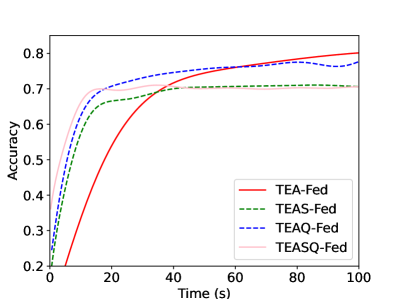
Figure 8: Ablation experiments of compression methods.

We further conduct ablation experiments on the used compression methods. In addition to the TEA-Fed (i.e., TEASQ-Fed without data compression), we evaluate the performance of our algorithm with only one single compression method, which is referred to as TEAS-Fed (i.e., TEA-Fed with sparsification) and TEAQ-Fed (i.e., TEA-Fed with quantization). In Figure 8, we show the accuracy of TEA-Fed, TEAS-Fed, TEAQ-Fed and TEASQ-Fed during the training progresses. According to the result, both TEAS-Fed and TEAQ-Fed with a single compression method can achieve faster training than TEA-Fed, and TEASQ-Fed which combines them can accelerate the training process more significantly. However, the performance of all methods with compression suffer from some degree of degradation, which is the cost of using compression.

Table 4: Time consumed to reach the target accuracy with IID data. “-” represents that the target is not achieved.

	81%	82%	83%	84%	85%	86%	87%	88%
FedAvg (IID)	45.26s	97.16s	134.01s	176.51s	205.15s	262.94s	-	-
TEA-Fed (IID)	55.73s	70.63s	84.82s	94.98s	102.58	116.37s	154.63s	233.47s
TEAStatic-Fed (IID)	75.63s	77.61s	82.59s	88.26s	104.32s	138.76s	-	-
TEASQ-Fed (IID)	63.48s	65.17s	67.5s	74.29s	95.3s	147.71s	290.28s	-

Table 5: The highest test accuracy within a given time budget using non-IID data.

	50s	100s	125s	150s	175s	200s	400s	600s
FedAvg (non-IID)	42.99%	47.84%	49.92%	52.69%	54.77%	58.22%	67.67%	71.66%
TEA-Fed (non-IID)	44.69%	57.54%	62.43%	65.91%	67.95%	70.01%	76.90%	79.52%
TEAStatic-Fed (non-IID)	37.33%	54.44%	60.45%	64.84%	67.03%	68.31%	73.73%	74.07%
TEASQ-Fed (non-IID)	47.94%	63.34%	66.85%	68.61%	70.26%	71.67%	75.04%	77.12%

Table 6: Time consumed to reach the target accuracy with non-IID data.

	68%	69%	70%	71%	72%	73%	75%	79%
FedAvg (non-IID)	402.71s	441.44s	483.52s	548.49s	-	-	-	-
TEA-Fed (non-IID)	193.47s	203.23s	224.49s	204.86s	220.72s	238.23s	307.11s	507.74s
TEAStatic-Fed (non-IID)	198.93s	208.6s	229.83s	238.23s	263.83s	288.92s	-	-
TEASQ-Fed (non-IID)	132.76s	150.10s	166.58s	202.43s	206.56s	306.27s	370.56s	-

5.2.5 Comparison with SOTAs

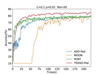
Figure 9: Comparison with asynchronous methods ASO-Fed, PORT and synchronous method MOON.

We compare our TEASQ-Fed with state-of-the-art baselines: asynchronous methods PORT ⁵⁴ and ASO-Fed ⁵⁵ as well as a synchronous method MOON ⁵⁶. As shown in Figure 9, TEASQ-Fed outperforms the other baselines in terms of the model accuracy, while it also has quicker convergence speed than most baselines except for PORT. Therefore, TEASQ-Fed has both advantages of accuracy and speed.

5.3 Discussion

Extensive experiments with diverse data distributions demonstrate that TEASQ-Fed has excellent performance for FL tasks and has significantly superior overall convergence than FedAvg and FedAsync. We summarize the improvements of TEASQ-Fed in the following three aspects:

• Faster convergence during model training. The asynchronous training mechanism makes it possible for more idle devices to participate in the training process, hastening the convergence of the model. The convergence speed of TEASQ-Fed is faster than the baseline methods, even if the $C$ value is larger.

• Higher convergence accuracy. We assign diverse importance based on the staleness of the updated local models during the model aggregation process. The rebalance of models improves the convergence rate and improves accuracy by reducing the impact of the staleness of local updates on the global model.

• Robust with heterogeneous data. TEASQ-Fed can achieve high convergence accuracy with highly heterogeneous data. With the regular penalty term within the local optimization on unbalanced data, we prevent divergence and increase the stability of the convergence of the global model. When dealing with non-IID data, the adjustment of the regularization value $\mu$ can lead to excellent performance in terms of both accuracy and convergence rate.

Table 7: The maximum storage space required during training.

	Global model	Local models
FedAvg (IID)	794.66KB	794.66KB
TEA-Fed (IID)	878.41KB	878.41KB
TEAStatic-Fed (IID)	575.70KB	496.53KB
TEASQ-Fed (IID)	529.77KB	498.92KB
FedAvg (non-IID)	794.66KB	794.66KB
TEA-Fed (non-IID)	878.41KB	878.41KB
TEAStatic-Fed (non-IID)	519.78KB	437.09KB
TEASQ-Fed (non-IID)	470.93KB	444.43KB

6 Conclusion

In this paper, we propose TEASQ-Fed, an innovative asynchronous federated technique with sparsification and quantization that intends to efficiently carry out FL training in edge computing. Through asynchronous training, TEASQ-Fed fully utilizes the downtime of edge devices, allowing more devices than with conventional methods to participate in the training process. In the meantime, TEASQ-Fed can significantly reduce the training time for the training process of FL and successfully minimize synchronization overhead. The extensive experimentation demonstrates that our approach has significant advantages with heterogeneous data in terms of accuracy (up to 16.67%) and training time (up to twice faster). The future scope of this work includes: (1) The investigation of the potential parallel training and transmission of different versions of models to further improve the efficiency of asynchronous FL; (2) The testbed experiment of the proposed algorithms to justify the performance in the real world.

References

- 1 Wang S, Tuor T, Salonidis T, et al. Adaptive federated learning in resource constrained edge computing systems. IEEE Journal on Selected Areas in Communications 2019; 37(6): 1205-1221.
- 2 Rawat W, Wang Z. Deep convolutional neural networks for image classification: A comprehensive review. Neural computation 2017; 29(9): 2352-2449.
- 3 Hard A, Rao K, Mathews R, et al. Federated learning for mobile keyboard prediction. arXiv preprint arXiv:1811.03604 2018.
- 4 Qi L, Liu Y, Zhang Y, Xu X, Bilal M, Song H. Privacy-aware point-of-interest category recommendation in internet of things. IEEE Internet of Things Journal 2022; 9(21): 21398–21408.
- 5 Liu Y, Zhou X, Kou H, et al. Privacy-Preserving Point-of-Interest Recommendation based on Simplified Graph Convolutional Network for Geological Traveling. ACM Transactions on Intelligent Systems and Technology 2023.
- 6 Yang Q, Liu Y, Chen T, Tong Y. Federated machine learning: Concept and applications. ACM Transactions on Intelligent Systems and Technology (TIST) 2019; 10(2): 1-19.
- 7 McMahan B, Moore E, Ramage D, Hampson S, Arcas yBA. Communication-efficient learning of deep networks from decentralized data. In: Artificial Intelligence and Statistics (AISTATS). Artificial Intelligence and Statistics. ; 2017: 1273–1282.
- 8 Liu J, Huang J, Zhou Y, et al. From distributed machine learning to federated learning: a survey. Knowledge and Information Systems 2022; 64(4): 885-917.
- 9 Liu J, Wu Z, Yu D, et al. Heterps: Distributed deep learning with reinforcement learning based scheduling in heterogeneous environments. FGCS 2023; 148: 106-117.
- 10 Zhou C, Liu J, Jia J, et al. Efficient device scheduling with multi-job federated learning. In: Proceedings of the AAAI Conference on Artificial Intelligence. AAAI. ; 2022: 9971–9979.
- 11 Mohammad U, Sorour S. Adaptive task allocation for asynchronous federated mobile edge learning. arXiv preprint arXiv:1905.01656 2019.
- 12 Li T, Sahu AK, Zaheer M, Sanjabi M, Talwalkar A, Smith V. Federated optimization in heterogeneous networks. Proceedings of Machine Learning and Systems 2020; 2: 429-450.
- 13 Xie C, Koyejo S, Gupta I. Asynchronous federated optimization. arXiv preprint arXiv:1903.03934 2019.
- 14 Stich SU, Cordonnier JB, Jaggi M. Sparsified SGD with memory. In: Advances in Neural Information Processing Systems (NeurIPS). NeurIPS. ; 2018.
- 15 Aji AF, Heafield K. Sparse communication for distributed gradient descent. arXiv preprint arXiv:1704.05021 2017.
- 16 Zhou C, Tian H, Zhang H, Zhang J, Dong M, Jia J. TEA-fed: time-efficient asynchronous federated learning for edge computing. In: ACM Int. Conf. on Computing Frontiers. ACM. ; 2021: 30-37.
- 17 Bouadjenek MR, Pacitti E, Servajean M, Masseglia F, Abbadi AE. A distributed collaborative filtering algorithm using multiple data sources. Int. Conf. on Advances in Databases, Knowledge, and Data Applications (DBKDA) 2018.
- 18 Chen J, Ran X. Deep learning with edge computing: A review. Proceedings of the IEEE 2019; 107(8): 1655-1674.
- 19 Liu J, Huang J, Zhou Y, et al. From distributed machine learning to federated learning: a survey. Knowledge and Information Systems 2022; 64(4): 885-917.
- 20 Wang X, Han Y, Wang C, Zhao Q, Chen X, Chen M. In-edge ai: Intelligentizing mobile edge computing, caching and communication by federated learning. IEEE Network 2019; 33(5): 156-165.
- 21 Chen J, Li K, Deng Q, Li K, Philip SY. Distributed deep learning model for intelligent video surveillance systems with edge computing. IEEE Transactions on Industrial Informatics 2019.
- 22 Li X, Huang K, Yang W, Wang S, Zhang Z. On the convergence of fedavg on non-iid data. arXiv preprint arXiv:1907.02189 2019.
- 23 Zhao Y, Li M, Lai L, Suda N, Civin D, Chandra V. Federated learning with non-iid data. arXiv preprint arXiv:1806.00582 2018.
- 24 Fu L, Zhang H, Gao G, Zhang M, Liu X. Client selection in federated learning: Principles, challenges, and opportunities. IEEE Internet of Things Journal 2023.
- 25 Nishio T, Yonetani R. Client selection for federated learning with heterogeneous resources in mobile edge. In: IEEE Int. Conf. on Communications (ICC). IEEE. ; 2019: 1-7.
- 26 Li C, Zeng X, Zhang M, Cao Z. PyramidFL: A fine-grained client selection framework for efficient federated learning. In: Proceedings of the 28th Annual International Conference on Mobile Computing And Networking. ACM. ; 2022: 158–171.
- 27 Xu C, Qu Y, Xiang Y, Gao L. Asynchronous federated learning on heterogeneous devices: A survey. Computer Science Review 2023; 50: 100595.
- 28 Nguyen J, Malik K, Zhan H, et al. Federated learning with buffered asynchronous aggregation. In: International Conference on Artificial Intelligence and Statistics. PMLR. ; 2022: 3581–3607.
- 29 Koloskova A, Stich SU, Jaggi M. Sharper convergence guarantees for asynchronous sgd for distributed and federated learning. Advances in Neural Information Processing Systems 2022; 35: 17202–17215.
- 30 Wu W, He L, Lin W, Mao R, Maple C, Jarvis S. Safa: a semi-asynchronous protocol for fast federated learning with low overhead. IEEE Transactions on Computers 2020; 70(5): 655-668.
- 31 Chen Y, Sun X, Jin Y. Communication-efficient federated deep learning with layerwise asynchronous model update and temporally weighted aggregation. IEEE Transactions on Neural Networks and Learning Systems 2019; 31(10): 4229-4238.
- 32 Su N, Li B. Asynchronous federated unlearning. In: IEEE INFOCOM 2023-IEEE Conference on Computer Communications. IEEE. ; 2023: 1–10.
- 33 Che T, Liu J, Zhou Y, et al. Federated Learning of Large Language Models with Parameter-Efficient Prompt Tuning and Adaptive Optimization. In: ACL special interest group on linguistic data (SIGDAT). ; 2023; Singapore.
- 34 Liu J, Zhou X, Mo L, et al. Distributed and deep vertical federated learning with big data. CCPE 2023: e7697.
- 35 Che T, Zhou Y, Zhang Z, et al. Fast federated machine unlearning with nonlinear functional theory. In: PMLR. ; 2023: 4241–4268.
- 36 Che T, Zhang Z, Zhou Y, et al. Federated Fingerprint Learning with Heterogeneous Architectures. In: IEEE. ; 2022: 31–40.
- 37 Liu J, Jia J, Ma B, et al. Multi-Job Intelligent Scheduling With Cross-Device Federated Learning. TPDS 2022; 34(2): 535–551.
- 38 Li G, Hu Y, Zhang M, et al. FedHiSyn: A Hierarchical Synchronous Federated Learning Framework for Resource and Data Heterogeneity. In: IEEE. ; 2022: 1-11.
- 39 Liu J, Che T, Zhou Y, et al. AEDFL: Efficient Asynchronous Decentralized Federated Learning with Heterogeneous Devices. In: IEEE. ; 2024: 1-15. to appear.
- 40 Li Q, Liu J, Sun Y, Zhang C, Dou D. On Mask-based Image Set Desensitization with Recognition Support. Applied Intelligence (APIN) 2024: 1-26.
- 41 Liu J, Jia J, Che T, et al. FedASMU: Efficient Asynchronous Federated Learning with Dynamic Staleness-aware Model Update. In: AAAI. ; 2024: 1-18. to appear.
- 42 Jin J, Ren J, Zhou Y, Lyu L, Liu J, Dou D. Accelerated Federated Learning with Decoupled Adaptive Optimization. In: PMLR. ; 2022: 1-25.
- 43 Xu H, Ho CY, Abdelmoniem AM, et al. Grace: A compressed communication framework for distributed machine learning. In: IEEE Int. Conf. on Distributed Computing Systems (ICDCS). IEEE. ; 2021: 561-572.
- 44 Xie C, Zheng S, Koyejo S, Gupta I, Li M, Lin H. Cser: Communication-efficient sgd with error reset. In: Advances in Neural Information Processing Systems (NeurIPS). NeurIPS. ; 2020: 12593-12603.
- 45 Basu D, Data D, Karakus C, Diggavi S. Qsparse-local-SGD: Distributed SGD with quantization, sparsification and local computations. In: . 32 of Advances in Neural Information Processing Systems (NeurIPS). NeurIPS. ; 2019: 1-12.
- 46 Jiang Y, Wang S, Valls V, et al. Model pruning enables efficient federated learning on edge devices. arXiv preprint arXiv:1909.12326 2019.
- 47 Zhang H, Liu J, Jia J, Zhou Y, Dai H. FedDUAP: Federated Learning with Dynamic Update and Adaptive Pruning Using Shared Data on the Server. In: Int. Joint Conf. on Artificial Intelligence (IJCAI). IJCAI. ; 2022: 2776-2782.
- 48 Zhang Z, Jin J, Zhang Z, et al. Validating the Lottery Ticket Hypothesis with Inertial Manifold Theory. In: Advances in Neural Information Processing Systems (NeurIPS). NeurIPS. ; 2021: 30196-30210.
- 49 Jiang Z, Xu Y, Xu H, Wang Z, Qian C. Heterogeneity-Aware Federated Learning with Adaptive Client Selection and Gradient Compression. In: IEEE INFOCOM 2023-IEEE Conference on Computer Communications. IEEE. ; 2023: 1–10.
- 50 Xu Y, Liao Y, Xu H, Ma Z, Wang L, Liu J. Adaptive control of local updating and model compression for efficient federated learning. IEEE Transactions on Mobile Computing 2022.
- 51 Shi W, Zhou S, Niu Z, Jiang M, Geng L. Joint device scheduling and resource allocation for latency constrained wireless federated learning. IEEE Transactions on Wireless Communications 2020; 20(1): 453-467.
- 52 Alistarh D, Grubic D, Li J, Tomioka R, Vojnovic M. QSGD: Communication-efficient SGD via gradient quantization and encoding. In: Advances in Neural Information Processing Systems (NeurIPS). NeurIPS. ; 2017: 1-12.
- 53 Xiao H, Rasul K, Vollgraf R. Fashion-mnist: a novel image dataset for benchmarking machine learning algorithms. arXiv preprint arXiv:1708.07747 2017.
- 54 Su N, Li B. How Asynchronous can Federated Learning Be?. In: IEEE/ACM Int. Symposium on Quality of Service (IWQoS). IEEE/ACM. ; 2022: 1-11.
- 55 Chen Y, Ning Y, Slawski M, Rangwala H. Asynchronous online federated learning for edge devices with non-iid data. In: IEEE Int. Conf. on Big Data (Big Data). IEEE. ; 2020: 15-24.
- 56 Li Q, He B, Song D. Model-Contrastive Federated Learning. In: IEEE/CVF Conf. on Computer Vision and Pattern Recognition (CVPR). IEEE/CVF. ; 2021: 10713-10722.