Flat bands without twists: periodic holey graphene
Abstract
Holey Graphene (HG) is a widely used graphene material for the synthesis of high-purity and highly crystalline materials. In this work, we explore the electronic properties of a periodic distribution of lattice holes, demonstrating the emergence of flat bands with compact localized states. It is shown that the holes break the bipartite sublattice and inversion symmetries, inducing gaps and a nonzero Berry curvature. Moreover, the folding of the Dirac cones from the hexagonal Brillouin zone (BZ) to the holey superlattice rectangular BZ of HG with sizes proportional to an integer times the graphene’s lattice parameter leads to a periodicity in the gap formation such that (mod ). Meanwhile, it is shown that if (mod ), a gap emerges where Dirac points are folded along the path. The low-energy hamiltonian for the three central bands is also obtained, revealing that the system behaves as an effective graphene material. Therefore, a simple protocol is presented here that allows obtaining flat bands at will. Such bands are known to increase electron-electron correlated effects. This work provides an alternative system, much easier to build than twisted systems, to obtain highly correlated quantum phases.
1 Introduction.
In recent years, the concept of electronic flat bands has gained prominence in the fields of materials science and condensed matter physics [1, 2, 3, 4, 5, 6, 7, 8, 9, 10]. This heightened interest can be attributed to the electronic, geometrical and topological properties inherent to flat bands [11, 12, 13, 10] and their potential to give rise to novel phenomena [14, 15, 7, 16, 17, 18, 19, 20]. Specifically, the discovery of superconductivity in twisted bilayer graphene (TBLG) in 2018 fueled considerable attention in the field [7]. However, the primary challenge lies in the experimental control of the rotation angle. For this reason, alternative systems are currently being explored to preserve flat bands, without relying solely on the rotation angle. Examples of these systems include graphene subjected to mechanical deformations [21, 22, 23, 24, 25, 26, 27, 28, 29] , multilayer graphene twisted (MTLG) under pressure [30, 31, 32, 33, 34], cyclicgraphyne, cyclicgraphdiyne [35] and holey graphene [36, 37, 38, 39], where the theoretical possibility of chiral superconductivity emergence has been demonstrated [40].
Holey Graphene (HG), also called Graphene Nanomesh (GNM), refer to the presence of holes distributed in the material [41, 37, 42, 43]. Introducing holes in graphene provides an additional degree of freedom to control optoelectronic and mechanical properties[44, 45, 46]. For example, holes create a mobility gap in graphene making it a narrow gap semiconductor [44]. This opens opportunities for exploring electronic, optical and correlated dependent phenomena and designing graphene-based devices that can exploit the unique properties of holey graphene [47, 48, 49, 50, 51].
Furthermore, the size and distribution of the holes can also modify the electronic properties. Using DFT calculations, Barkov et al. [52] investigated holey graphene’s transmission function, . They found that introducing periodic holes can modulate the values of by changing the distances between holes and maintaining the hole size; thus, the conductance tends to increase farther apart.
In addition, several techniques are employed to fabricate HG, including electron/ion beam lithography [48, 53, 47], plasma etching [48, 47], chemical etching [37], laser-based methods [54, 55, 56, 57, 58, 59], and others [43, 60, 48, 47, 61, 51, 49, 62, 63, 64] . These techniques offer an experimental advantage over MTLG. Among them, the most common techniques used to fabricate HG are:
Top-down lithography involves the selective removal of graphene sheets to create nanopores with uniform sizes and spatial arrangement. Although successful in producing graphene sheets with uniform nano-size pores, this technique faces challenges in large-scale fabrication and requires specialized equipment and expertise, making it expensive [48, 53, 47].
Another technique used to fabricate HG is template-assisted chemical vapor deposition [48, 53, 51, 62]. In this method, HG is grown on specific inorganic templates. This technique allows for the bottom-up growth of HG and offers control over nanopores’ size, shape, and distribution [62]. However, these fabrication techniques have certain drawbacks because they require careful control of various parameters such as temperature, pressure, and duration, making the process lengthy, cumbersome, and costly.
A third approach to synthesizing HG is using block copolymer lithography techniques on CVD-grown graphene [60, 65]. This technique involves patterning the graphene with a copolymer material and using reactive ion etching to create nanopores in the desired arrangement. One advantage of this technique is that it allows for the control of the neck width, which can be important in determining the properties and applications of HG. However, this approach still requires further optimization to achieve large-scale production of HG.
Nevertheless, laser-based methods have recently emerged as a promising technique for synthesizing HG [54, 55, 56, 57, 58, 59]. These methods offer a precise means of controlling the synthesis process of the holey structure. Researchers can adjust parameters like laser intensity and target material to create holes with specific sizes, shapes, and distributions. This level of control enables the production of HG with tailored properties for various applications. Moreover, this method allows for the fabrication of high-purity and highly crystalline HG without the need for catalysts or chemicals. Laser ablation methods are also scalable, making them ideal for large-scale HG production. Furthermore, these techniques permit the customization of HG by introducing dopants and functional groups. This versatility contributes to the development of graphene-based devices with enhanced performance. However, it’s worth noting some notable disadvantages, including the cost and complexity of the equipment, limited scalability for large-area synthesis of pristine graphene, and challenges in achieving structural uniformity.
In this work, we explore different configurations of holey graphene which we show are able to produce flat-bands. From there, we study its electronic properties of the resulting lattices. The structure of this work is as follows: in Section 2, we present the tight-binding model and the unit cells of the holey graphene primarily under discussion. In Section 3 we present the electronic properties of the systems introduced in Section 2. Therein, the emergence of flat bands with compact localized states and energy gaps is discussed in terms of the Brillouin zone folding and bipartite sublattices site imbalance. Finally, our conclusions and future perspectives are outlined in Section 4.
2 Tight-binding holey graphene model
Our model is based on periodically distributed holes within a graphene lattice, maintaining translational symmetry. This enables us to simplify the treatment by leveraging Bloch’s theorem. As seen in Fig. 1 a), we use a 4-atom superlattice unit cell containing the usual graphene non-equivalent sites and , where and refer to carbon atoms on each of the graphene’s bipartite lattices, distinguished in the figure by colors blue and red, respectively.
Additionally, we use two orthogonal lattice vectors: and , where Å is the carbon-carbon distance. As visually depicted in Fig. 1 a) and b), this specific configuration ensures the alignment of the horizontal axis with the zigzag orientation and the perpendicular axis with the armchair orientation.
a) 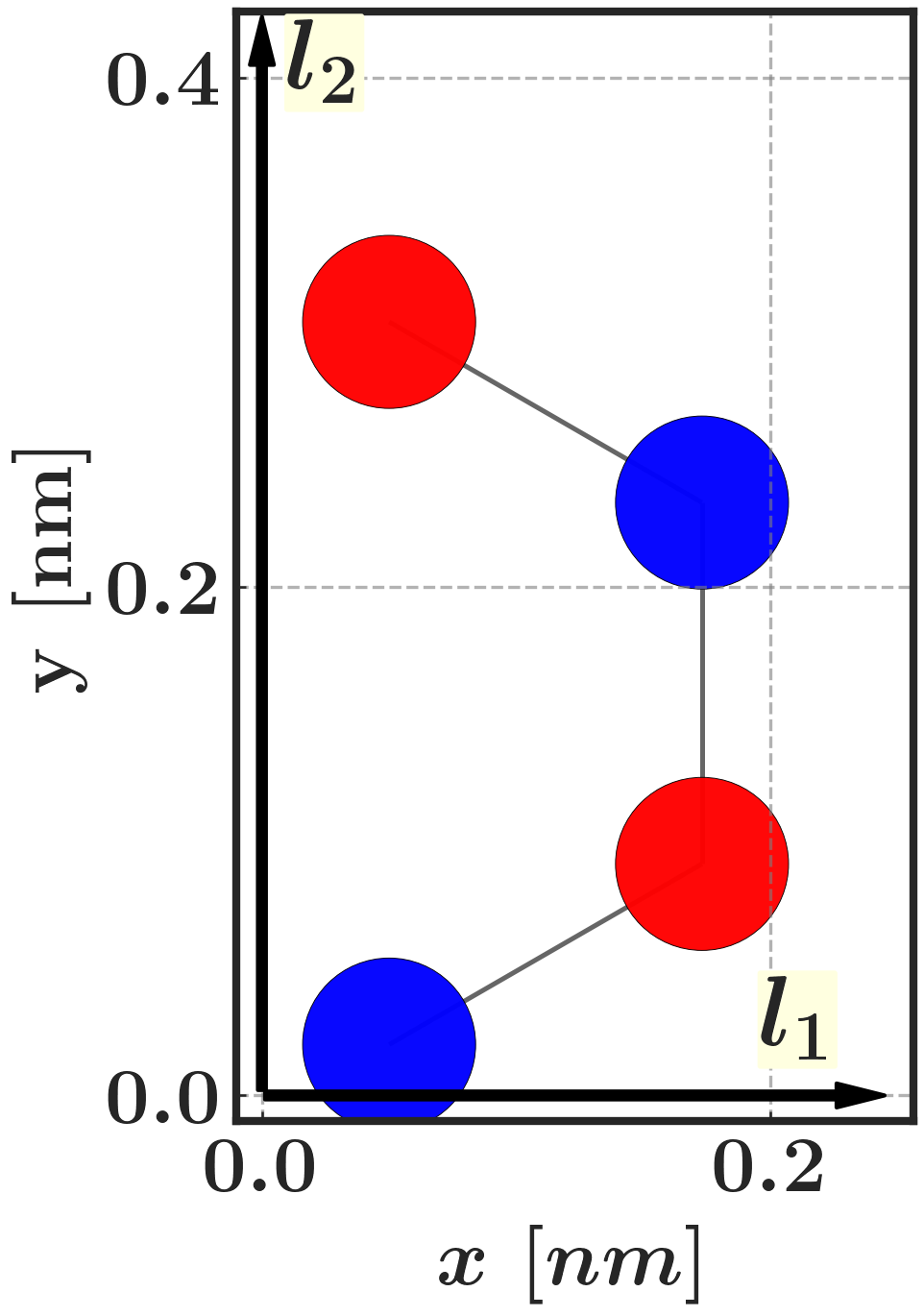 b)
b) 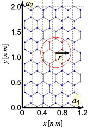 c)
c) 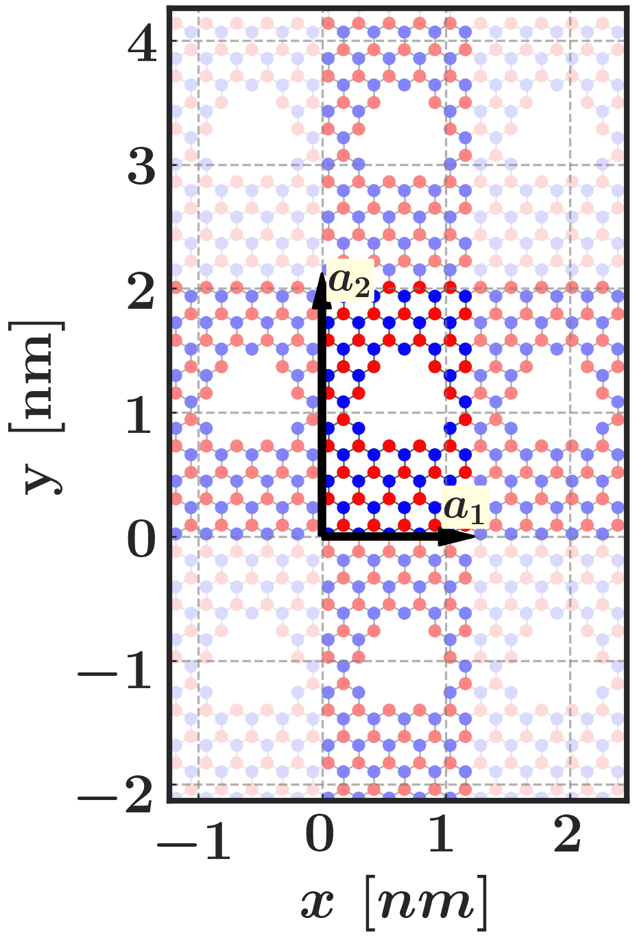
d) 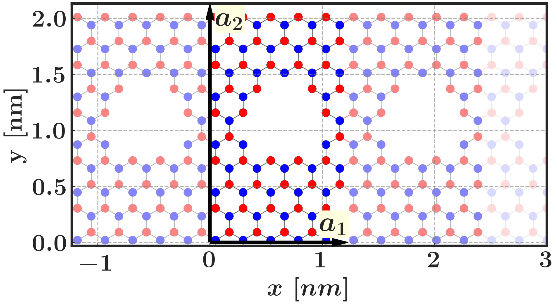 e)
e) 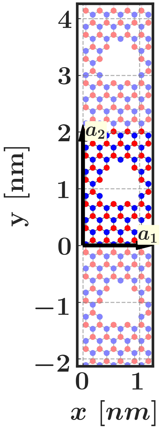
After obtaining the graphene lattice, we selectively remove atoms located within circles of radius (Å) (refer to Fig. 1c). We define the unit cell by employing lattice vectors and (as shown in Fig. 1b), where to ensure periodicity in the direction, and similarly, is employed to establish periodicity in the direction. It is worth noting that, without loss of generality, the circle delineating the atoms for removal is centered at . As depicted in Fig. 1, we obtain a lattice featuring holes; and cutting exclusively in the horizontal or vertical direction results in nanoribbons with zigzag or armchair boundaries, respectively (refer to Fig. 1d and e). We will denote the unit cell of graphene with a hole of radius and vectors as UCHG, and correspondingly, the nanoribbons with zigzag and armchair directions as ZHGN and AHGN, respectively.
Under such considerations, our investigation is based on a tight-binding model with only first-neighbors hopping transfer integral, which yields a Hamiltonian given by
| (1) |
where represents the sum over the neighbors with positions and that satisfy ; is the creation (annhilation) operator and eV is the hopping integral between the -th and -th sites. Additionally, we numerically construct the Hamiltonian operator in reciprocal space , which depends on the number of atoms in the unit cell and is denoted as . The eigenvalues and eigenfunctions were thus numerically found by using python dedicated libraries [66, 67, 68]. In the following section we will discuss the resulting electronic and optical properties.
3 Electronic properties of bidimensional Holey Graphene
a)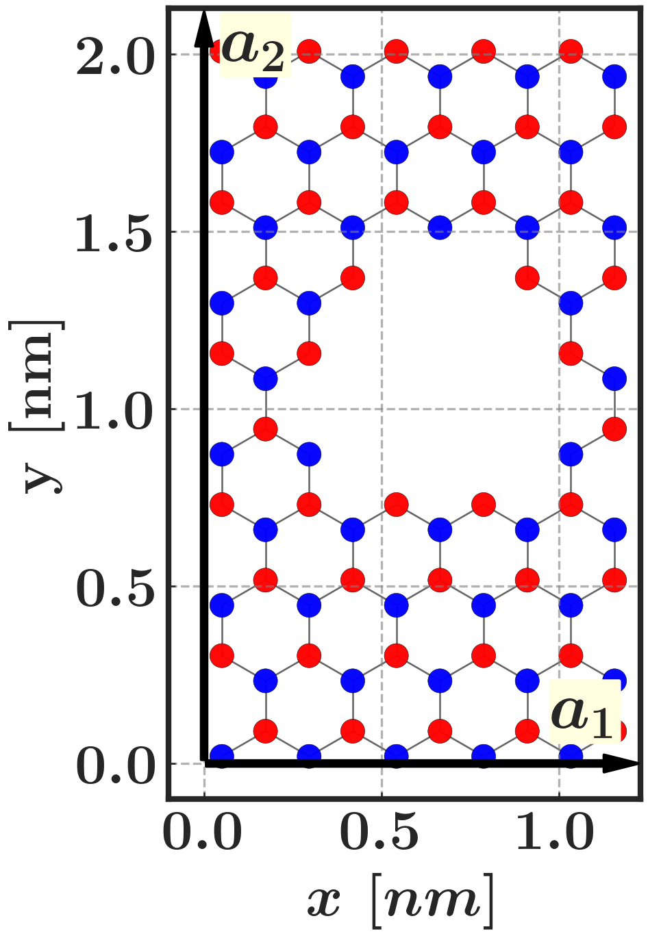 b)
b) 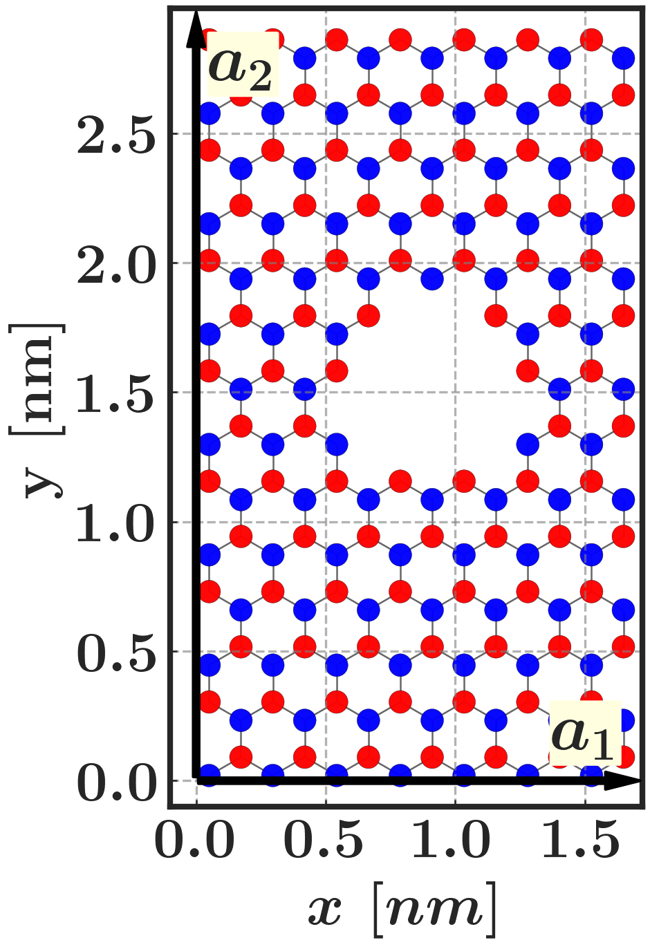 c)
c) 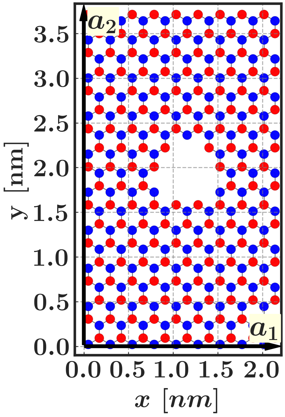
d) 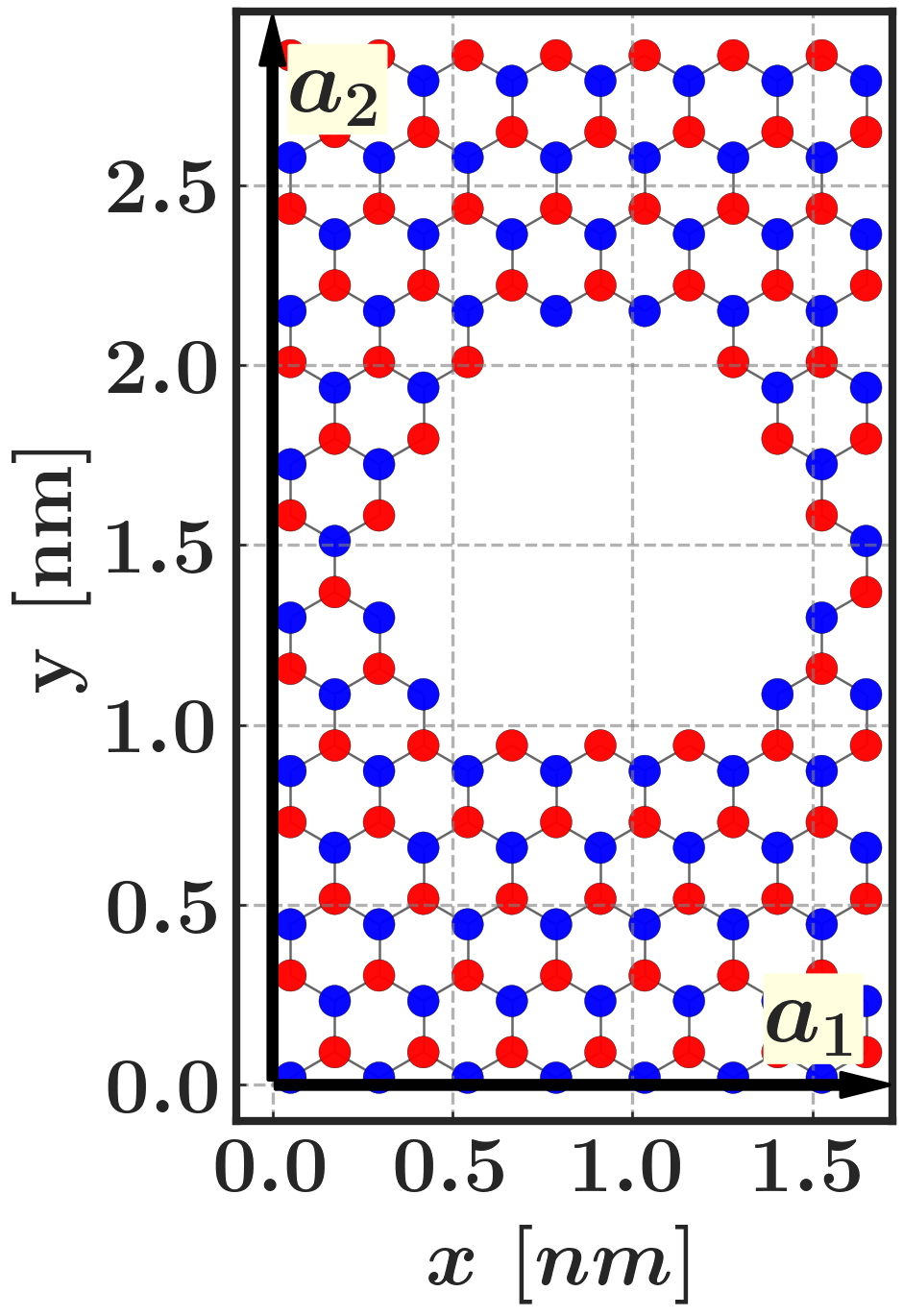 e)
e) 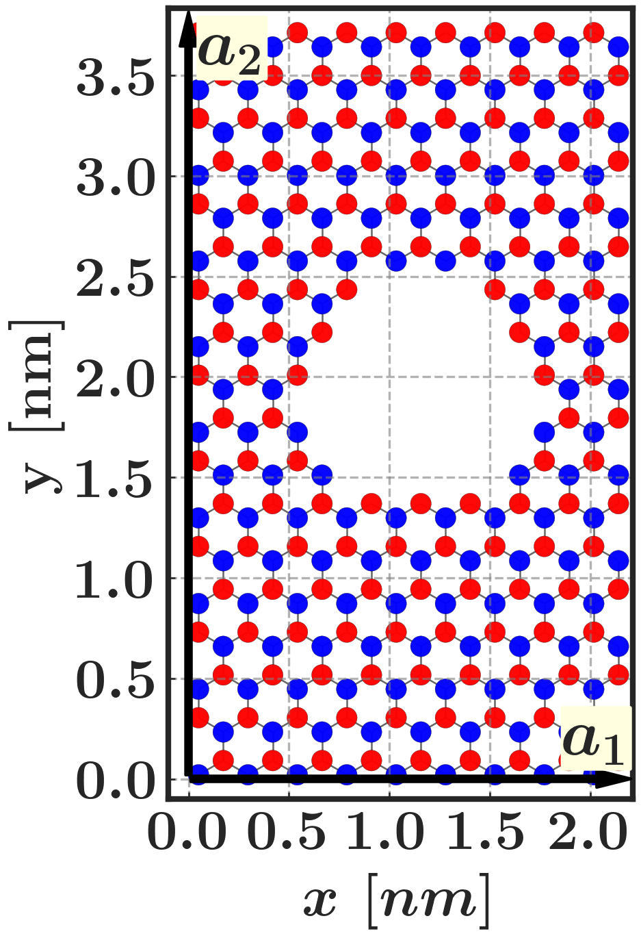 f)
f) 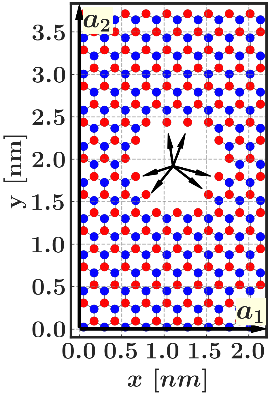
a) 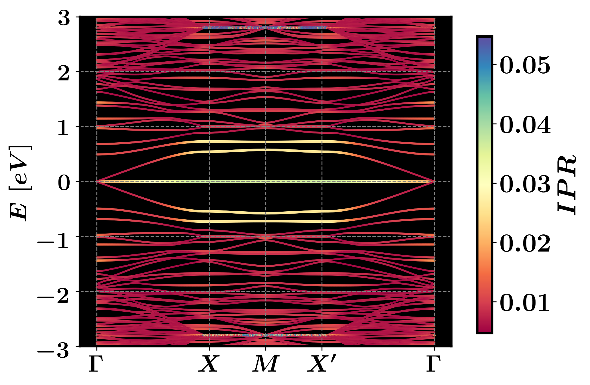 b)
b)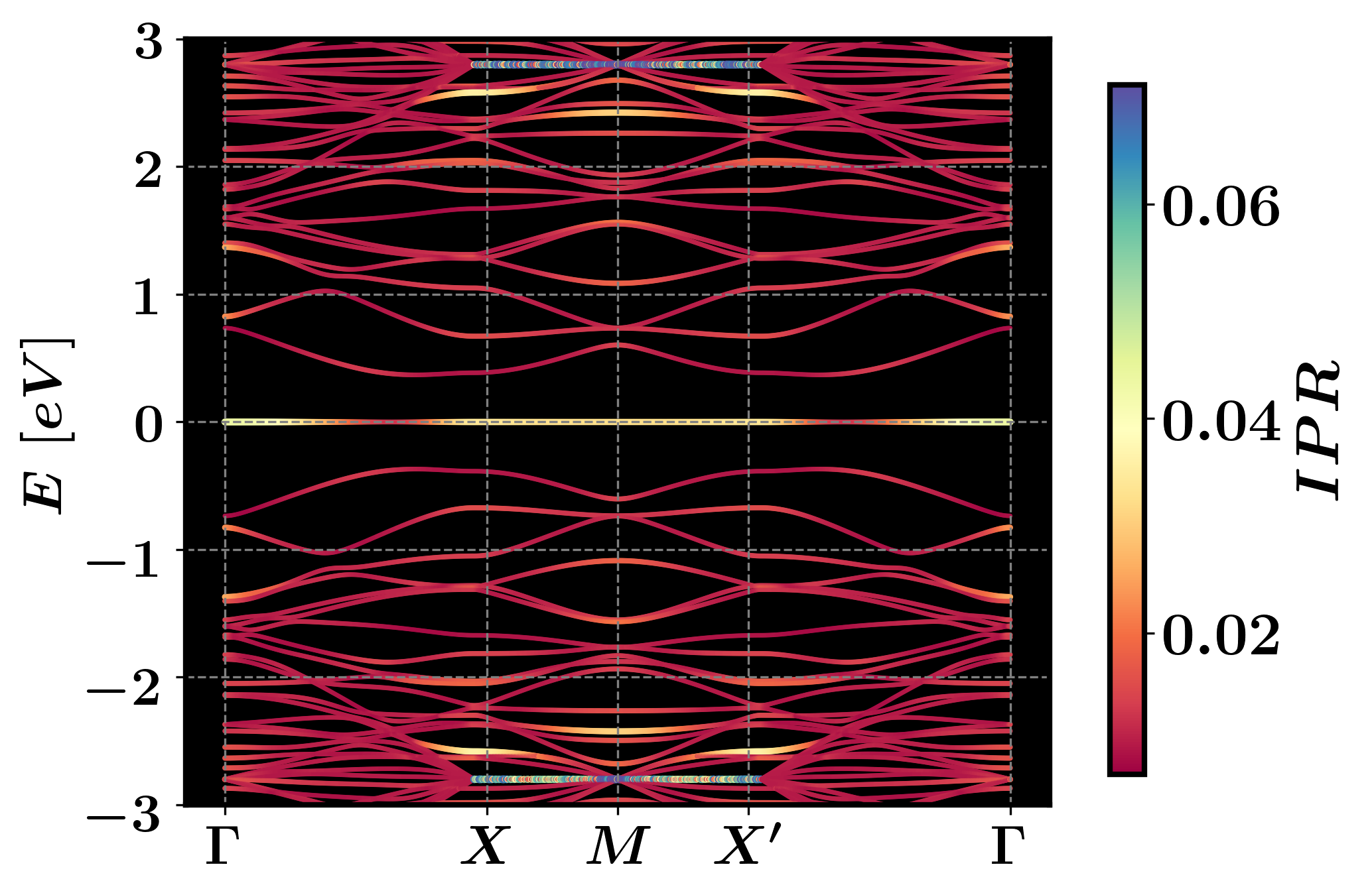
c)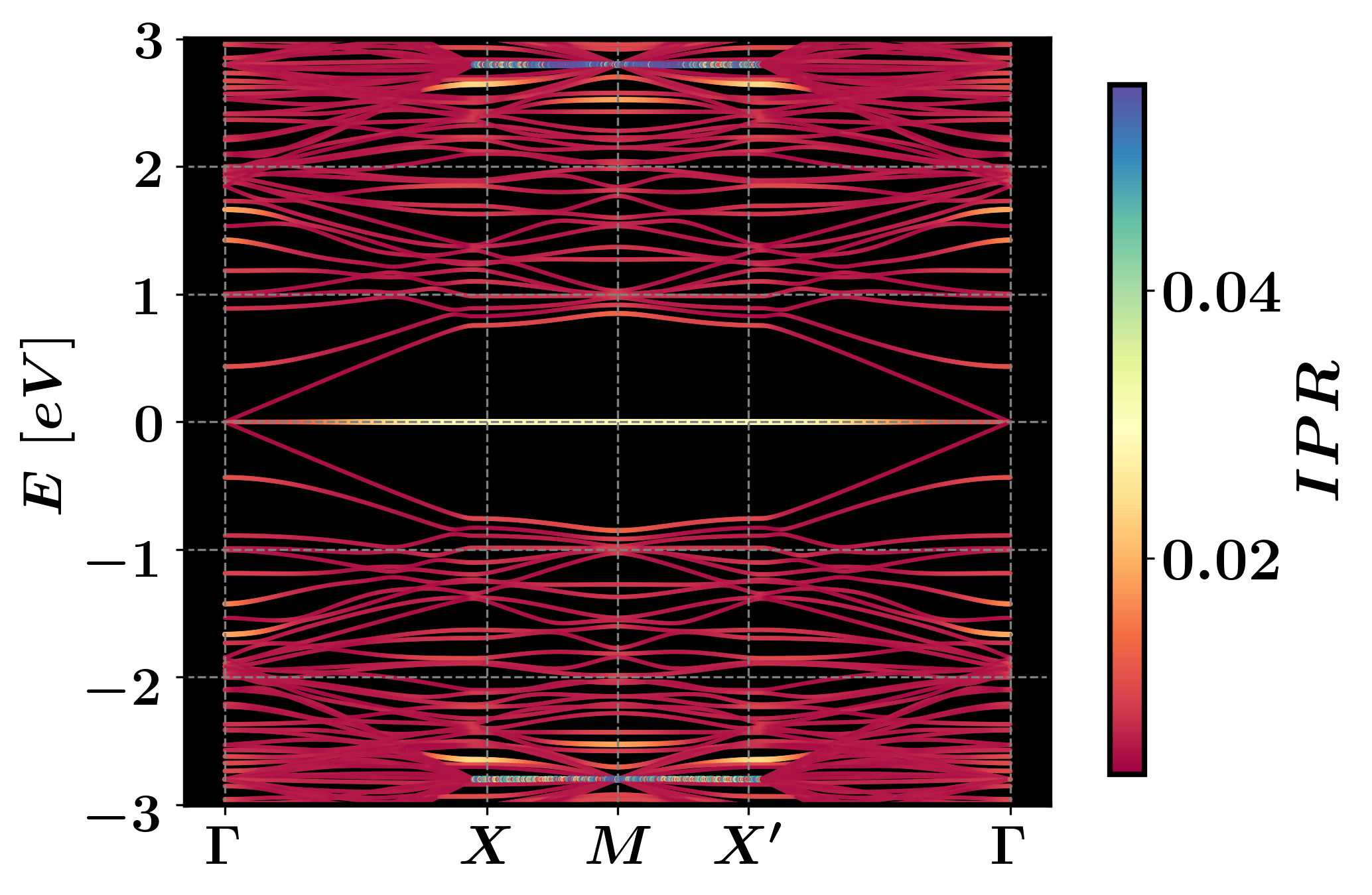 d)
d)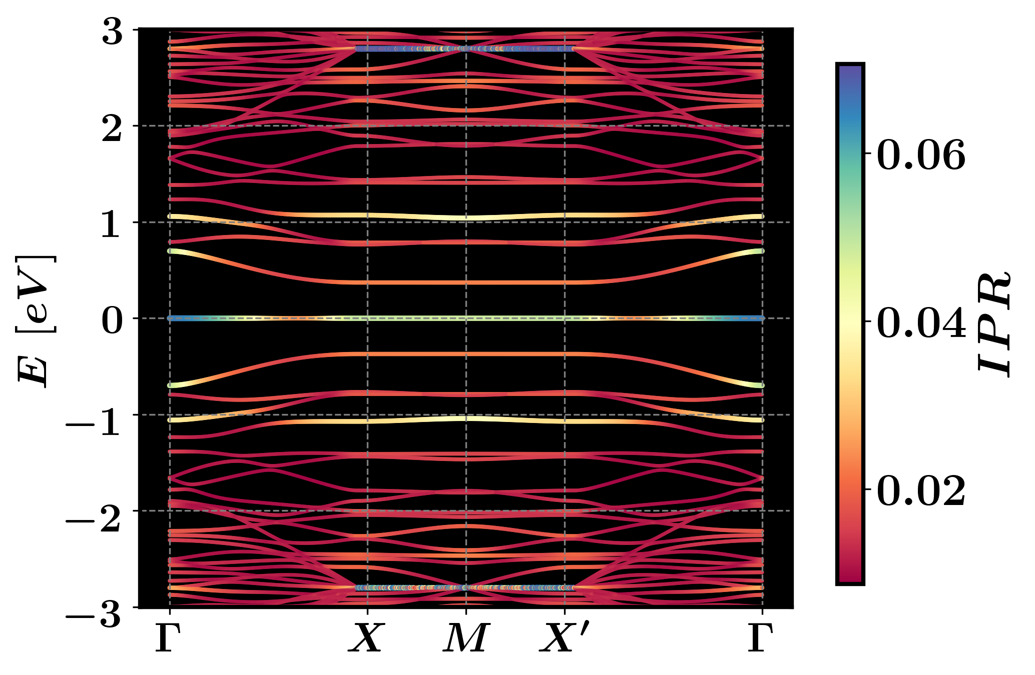
e)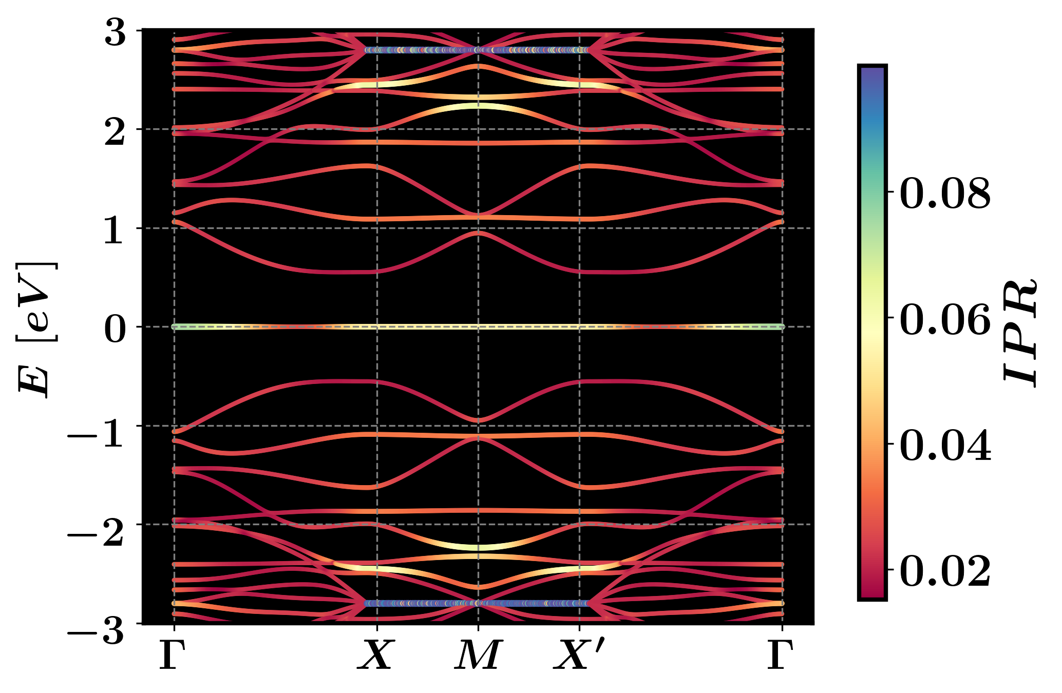 f)
f)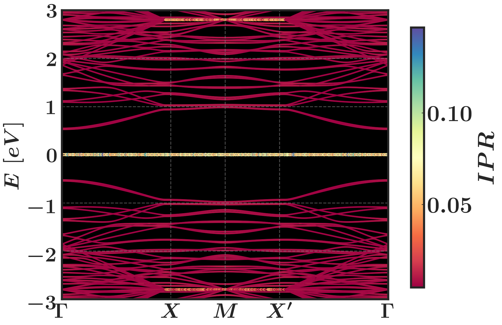
In this section, we will discuss the electronic and optical properties of systems with unit cells of type UCHG, focusing primarily on those depicted in Figure 2, namely, UCH, UCHG, UCHG, UCHG, UCHG, and UCHG. These examples were chosen to include the effects of different radius and edge terminations. Observe that among our examples, in Fig. 2 f) we include the case of a hole with dangling bonds.
In Fig. 3 we illustrate the bands obtained for each of the systems shown in Fig. 2. As we can see, gaps are observed in some cases while Dirac cones are seen in others. The opening of these gaps will be discussed later on in this section. Meanwhile, we observe that at energy flat bands are obtained in all cases, corresponding to the Fermi energy ( eV) at half-filling. Recent research suggests that the formation of flat bands is intricately linked with Compact Localized States (CLS) [10], also known as confined states [70, 71], signifying the existence of a non-trivial localization behavior.
In order to ascertain whether there exists differences in the localization properties of states within the flat bands and those outside of them, we employ the Inverse Participation Ratio (IPR) [72, 73, 74, 44, 75]
| (2) |
where represents the wave function in the -th bands and characterized by momentum and energy , and due to the periodic condition of the lattice, we perform the integral over the unit cell (UC). The IPR of an extended state goes as where is the number of extended states, while for localized states does not depend on . For exponentially localized states, it can be proven that where is the localization length,.
a) 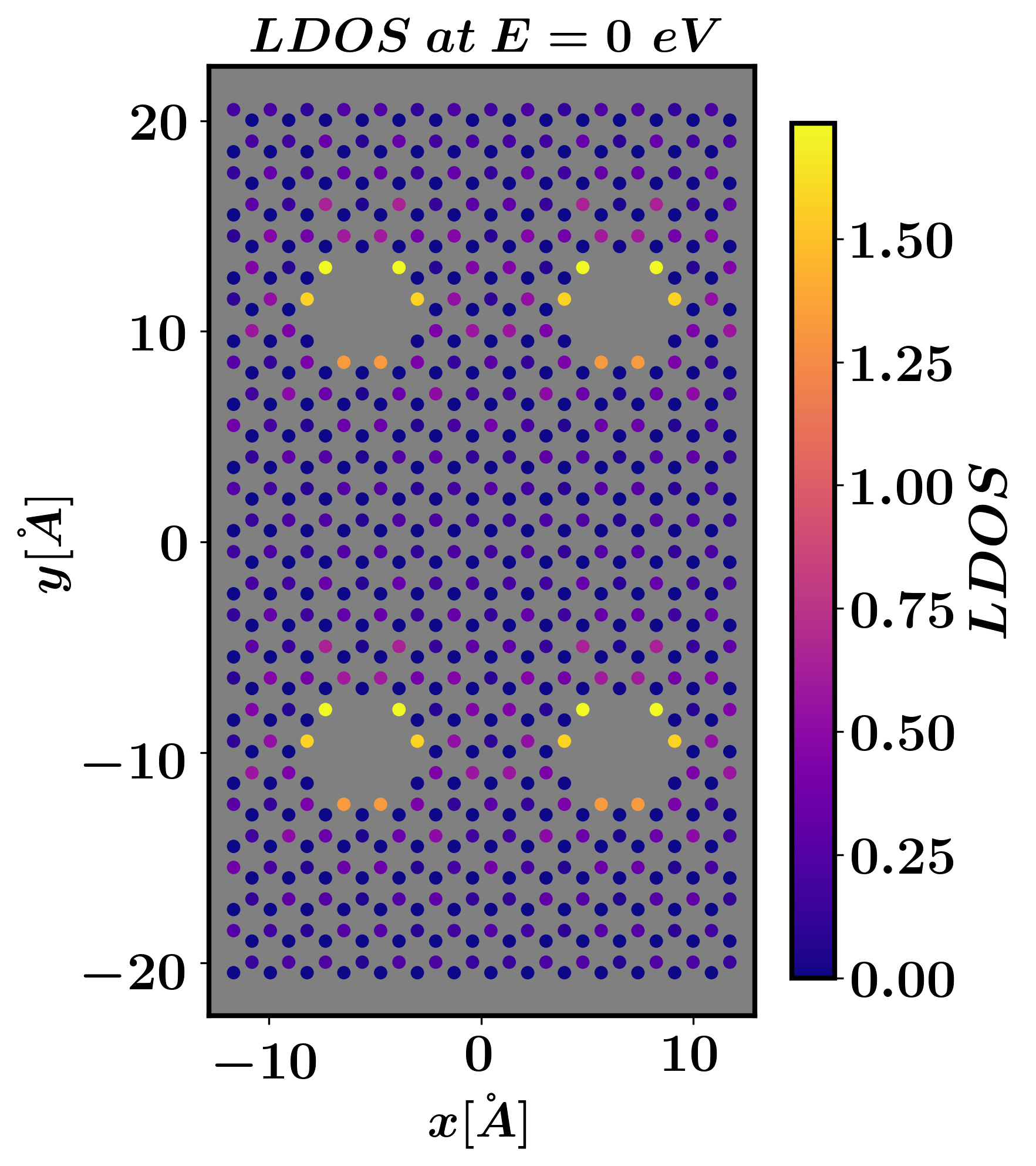 b)
b)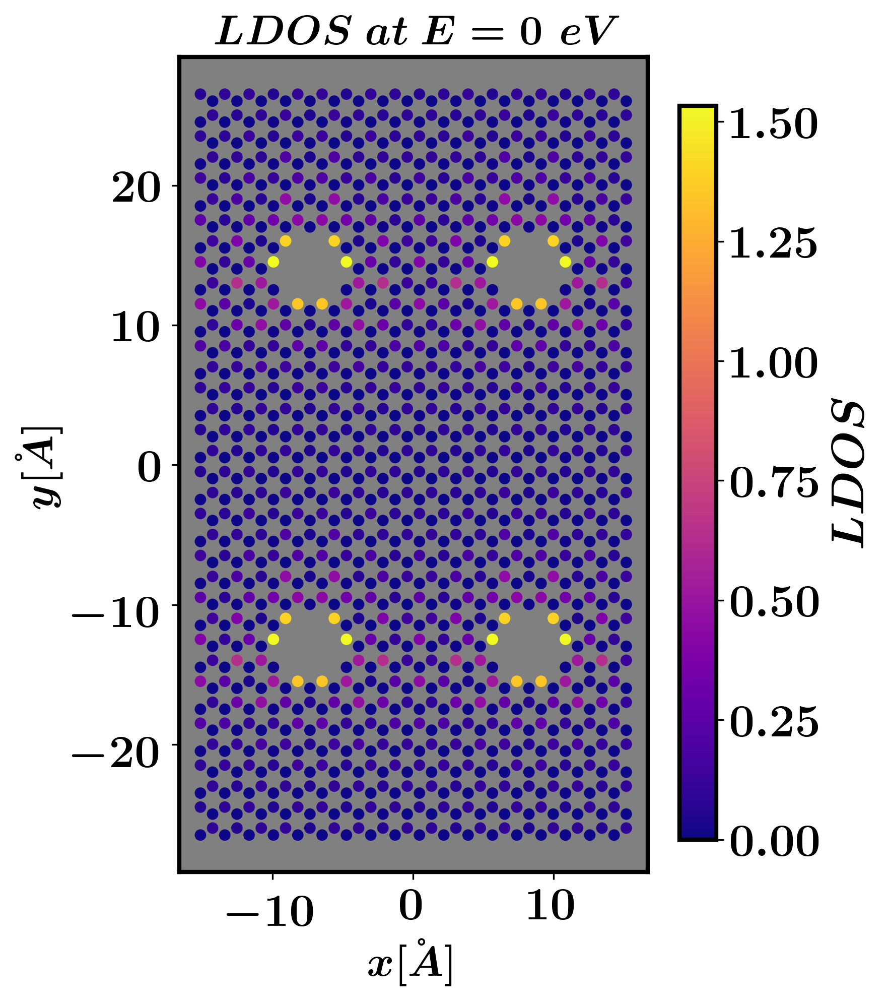 c)
c) 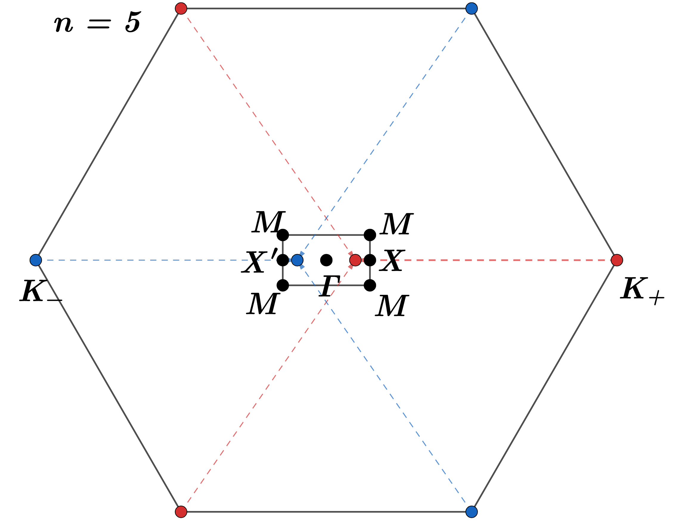
d) 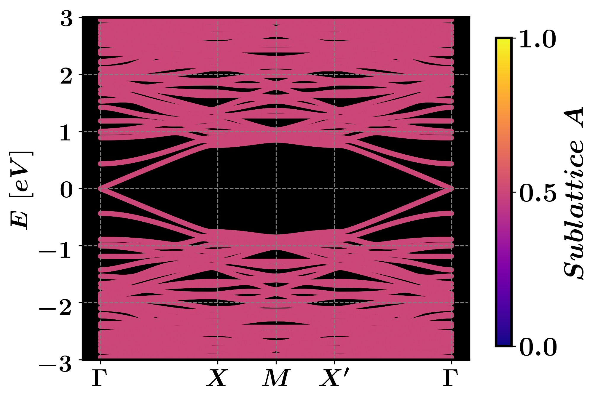 e)
e) 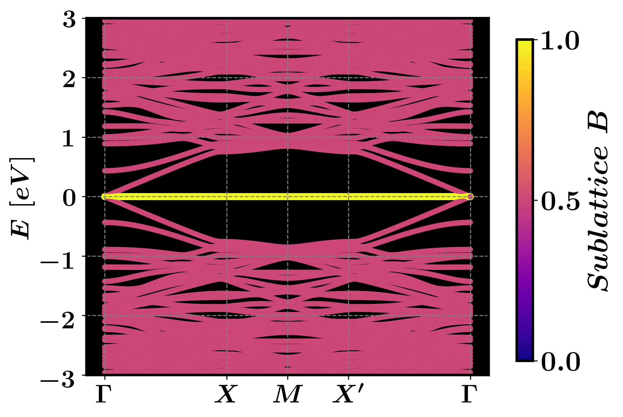
f) 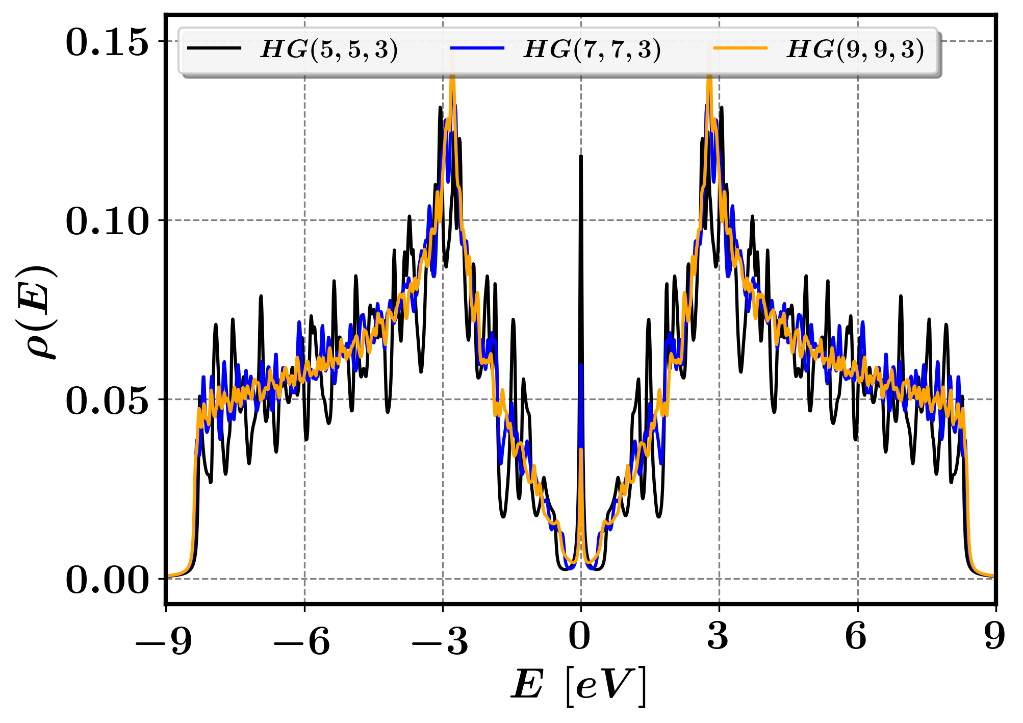 g)
g) 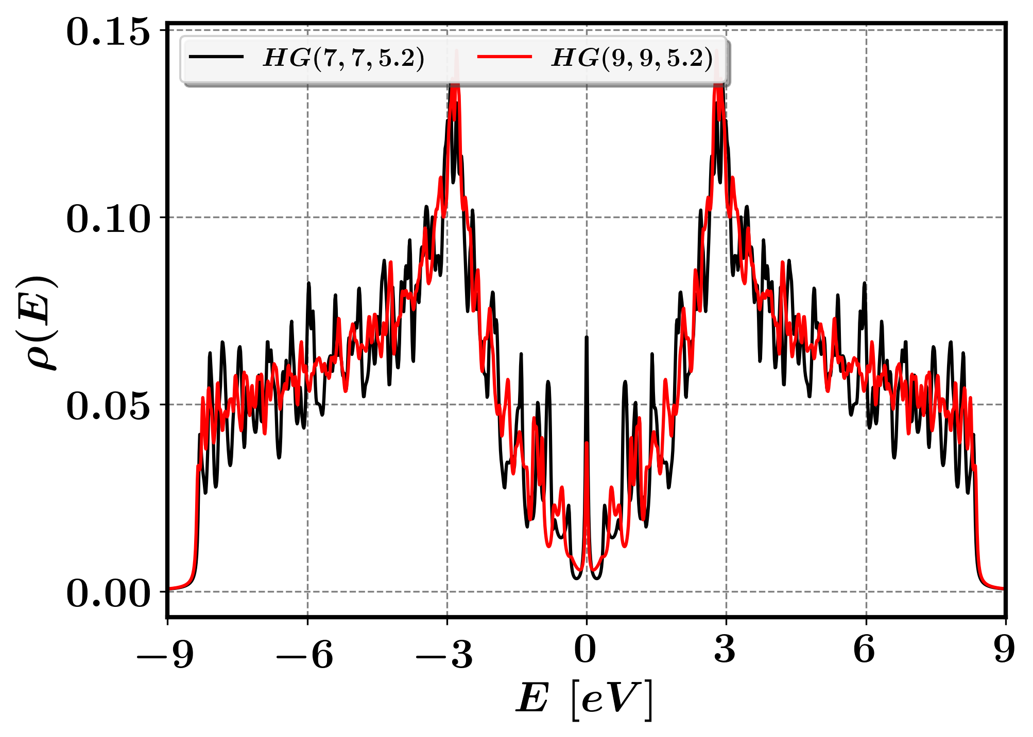
In Figure 3, the values for each are projected onto the band structure using a color code. As anticipated, the flat band states exhibit a significantly high degree of localization in contrast to the majority of other states. Flat band states preferentially spatially localize in the zig-zag boundary regions that form around the hole, as can be observed in Figure 4 a) and b). However, it is worth noting that these localized states are not the sole examples; in addition, we find states for which the bands exhibit quasi-flat behavior within specific regions of the Brillouin zone, notably those with energies at and momenta between the and points. Such behavior is due to the presence of Van Hove singularities in which a dimerization effect is seen [8, 77, 29].
To further confirm the nature of localization, in Fig. 3 a)-b) we present the local density of states (LDOS) for a flat band state as a function of the sites for two different examples. Therein it can be seen that localization mainly occurs at the edges of the holes as expected. Also, from Figs. 3 a)-d) and 4 a) and b), it is observed that if increases while remains constant, or vice versa, the localization in the flat band decreases. However, for and such rule does not to hold since in addition to a increased localization, a gap opens. To gain a better understanding on the formation of flat bands, the gap size, and the density of states at , we introduce two parameters. The first one is the imbalance number, denoted as , given by
| (3) |
which indicates the difference between number of sites and in the unit cell UCHG. The second is the imbalance density, , given as
| (4) |
where is the total number of atoms in each unit cell.
As established in Ref. [78], sublattice site imbalance in bipartite lattices can induce flat bands of confined states, and in certain cases, the formation of energy gaps and pseudogaps. Bipartite sublattice site imbalance will occur here only at hole edges. To see if such effect is in play , in Table 1 we present the values for the site imbalance number, the site imbalance density, the energy gap, the density of states (DOS) at and the observed number of flat bands.
From Table 1, we conclude that the number of flat bands formed at energy eV coincides with the imbalance number for all the studied cases. In recent studies, it has been demonstrated that the formation of degenerate flat bands is also a consequence of a broken path-exchange symmetry [76, 10]. Upon breaking, this symmetry introduces a complex phase [76, 10], leading to the lifting of the degeneracy while simultaneously preserving the flatness of the band. In the periodic holey system presented here, it can be demonstrated that the number of imbalances is related to the path exchange symmetry, and consequently the number of flat bands is equal to the imbalance number. Specifically, when such symmetry is broken and an isolated flat band emerges. Therefore, such symmetry distinguishes the sublattice with the highest number of sites. This is illustrated in Fig. 4, panels d) and e), for the case of HG, where the nonzero energy bands result from equal contributions from sublattices and .
Additionally, it is worth noting that the density of states (DOS or ), at is directly proportional to the imbalance density (see Table 1). In cases where there are no dangling bonds, we observe that , while in cases with dangling bonds, we find that (see Fig. 4 f) and g)). This can be understood by considering the DOS for each unit cell, in this case, , where is the number of sites supporting the state with . Therefore, . In the studied cases without dangling bonds, fluctuates between sites (see for example Fig. 4 a) and b)), and , maintaining an average ratio of (see Table 1 and Fig. 4 f) and g) ). For cases with dangling bonds, the state is strongly localized on these dangling sites, and corresponds to this number of sites, hence .
| [Å] | [eV] | No. Flat Bands | ||||
Let us know discuss the origin of the gaps. In Fig. 5 we present the gap sizes for three distinct graphene series with hole radii of Å, respectively. For each of these series, the size of the unit cell,, is considered within the range of values , with the exception of the first series where . The initial observation of note in Fig. 5 is that, for the series featuring hole radii of and Å, a periodicity with the property emerges for sufficiently large values relative to the specific value at which the gap reaches zero. This phenomenon is particularly evident in Figure 3 c) and e), where the emergence of Dirac cones at the points is clearly observed. To understand the origin of the gaps, we rely on Fig. 5, and excluding the semimetallic cases, it is obtained that in the three series the gap size, , follows a power law as a function of the imbalance density , where is approximately , , and for the respective series. These values, close to , are comparable to the case where there is a density of impurities breaking the sublattice symmetry, and the imbalance density is given by . In a previous work [44], it was found analytically that . The nearly similar exponents indicate that in the end, big holes enter as effective impurities and that the mechanism of underlying frustration due to sublattice imbalance is in play here [44].
a) 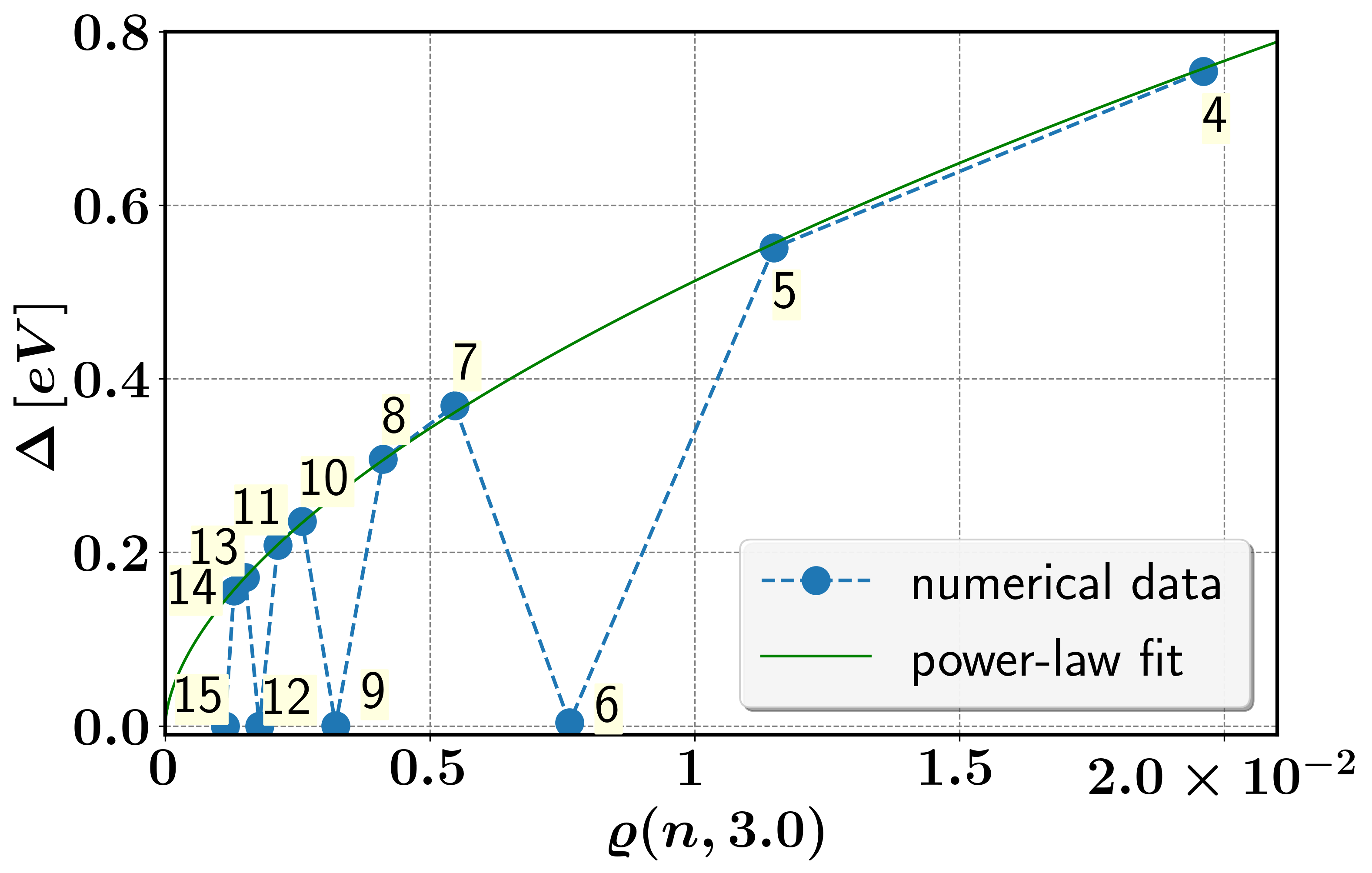 b)
b)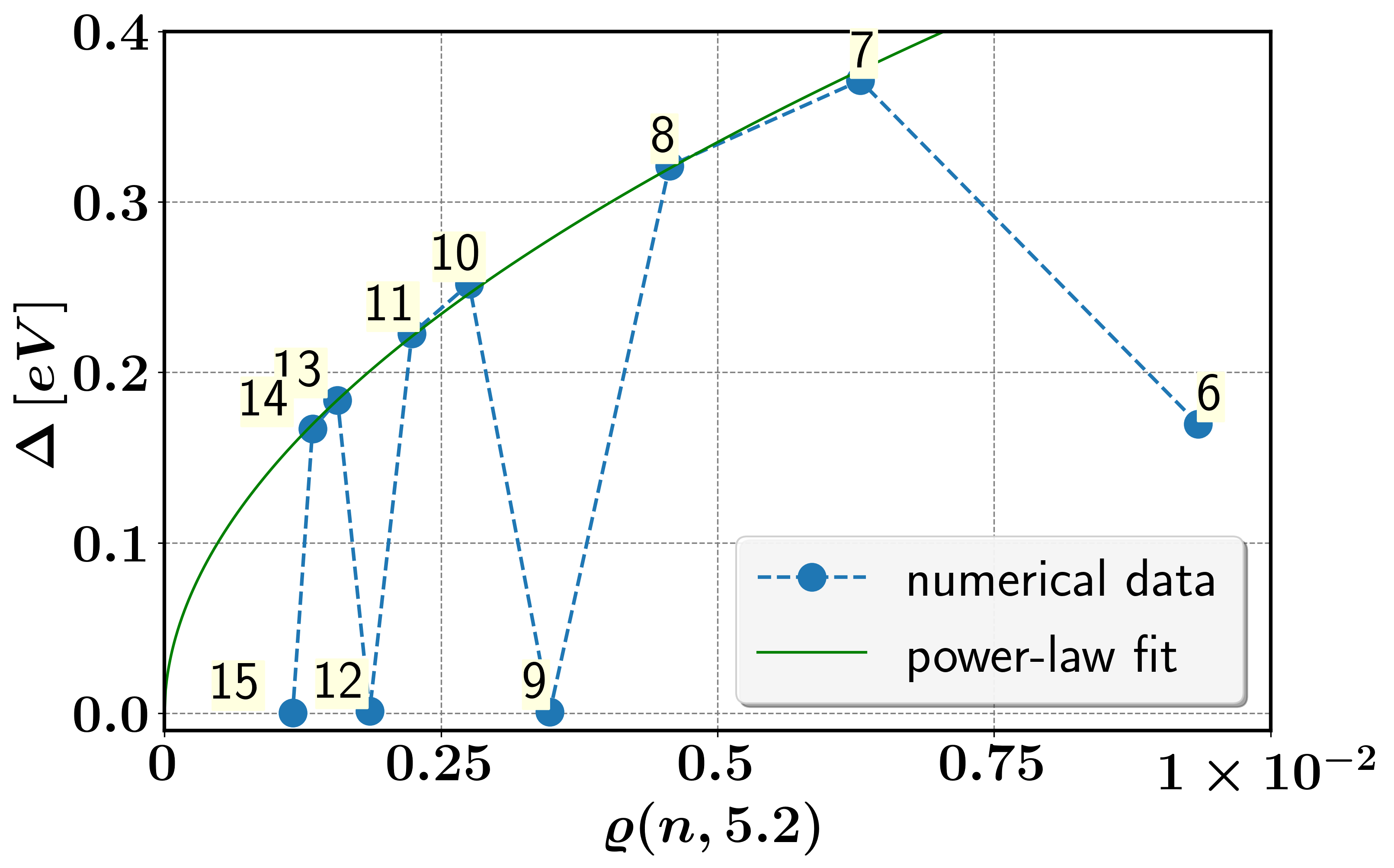
c) 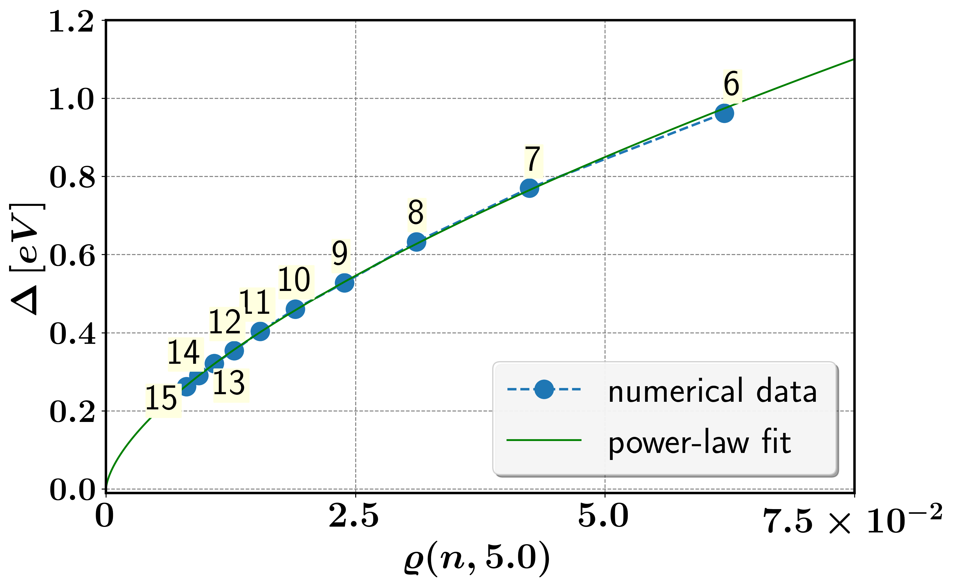
On other hand, we will now demonstrate that gap periodicity arises due to the folding of the Dirac cones from the pristine graphene hexagonal Brillouin zone to the holey superlattice rectangular Brillouin zone (see Fig. 4 c) and from broken symmetries. To do this, consider the original Dirac points on each of graphene’s valley,
| (5) |
in the hexagonal Brillouin zone of graphene and is the valley pseudospin index. On other hand, the reciprocal vectors
| (6) |
of holey graphene with UCHG. It can be demonstrated that if with and , the following equation is obtained,
| (7) |
a)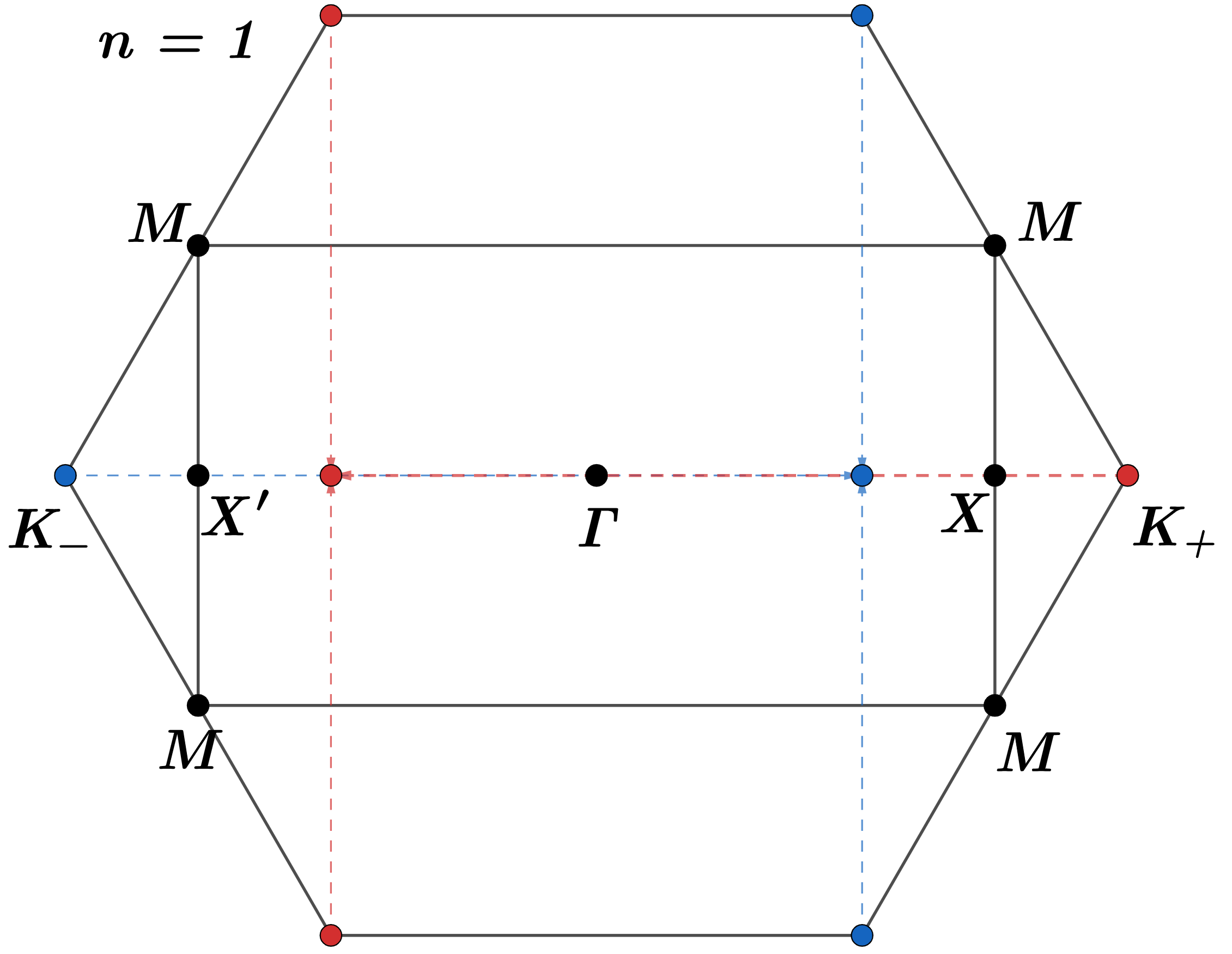 b)
b) 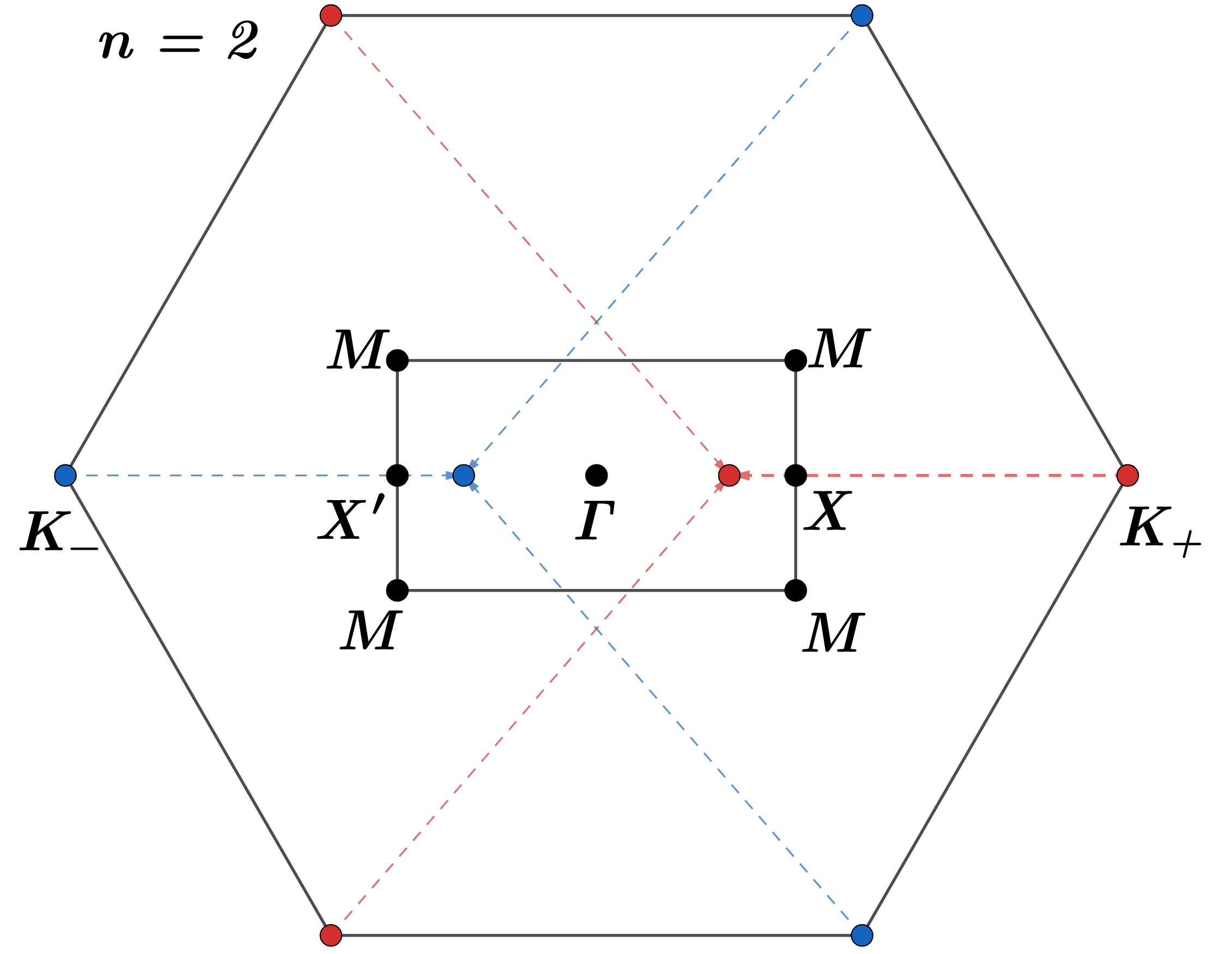
c) 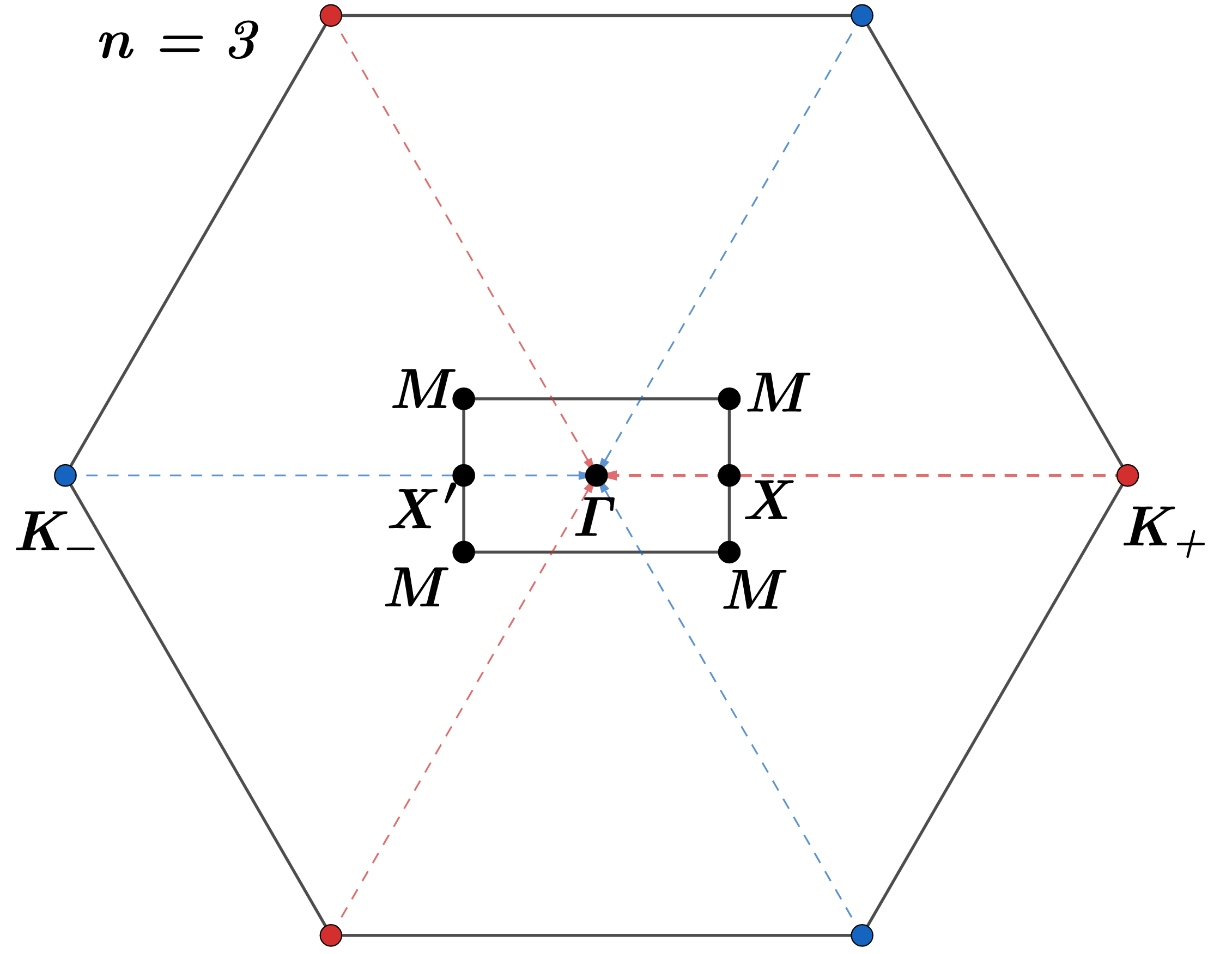 d)
d) 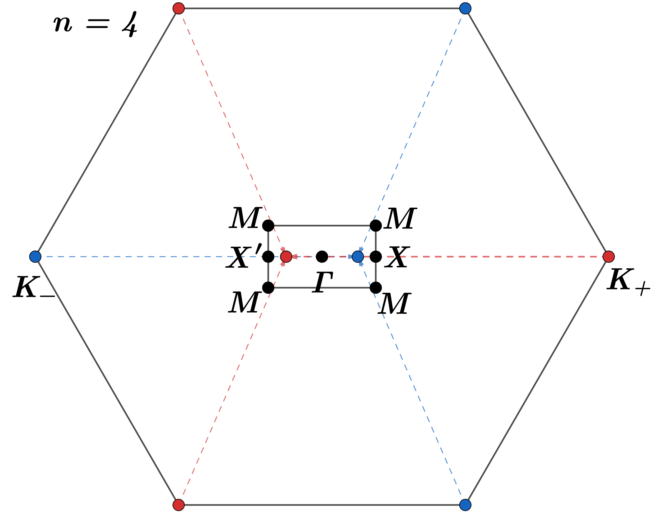
e)
f) 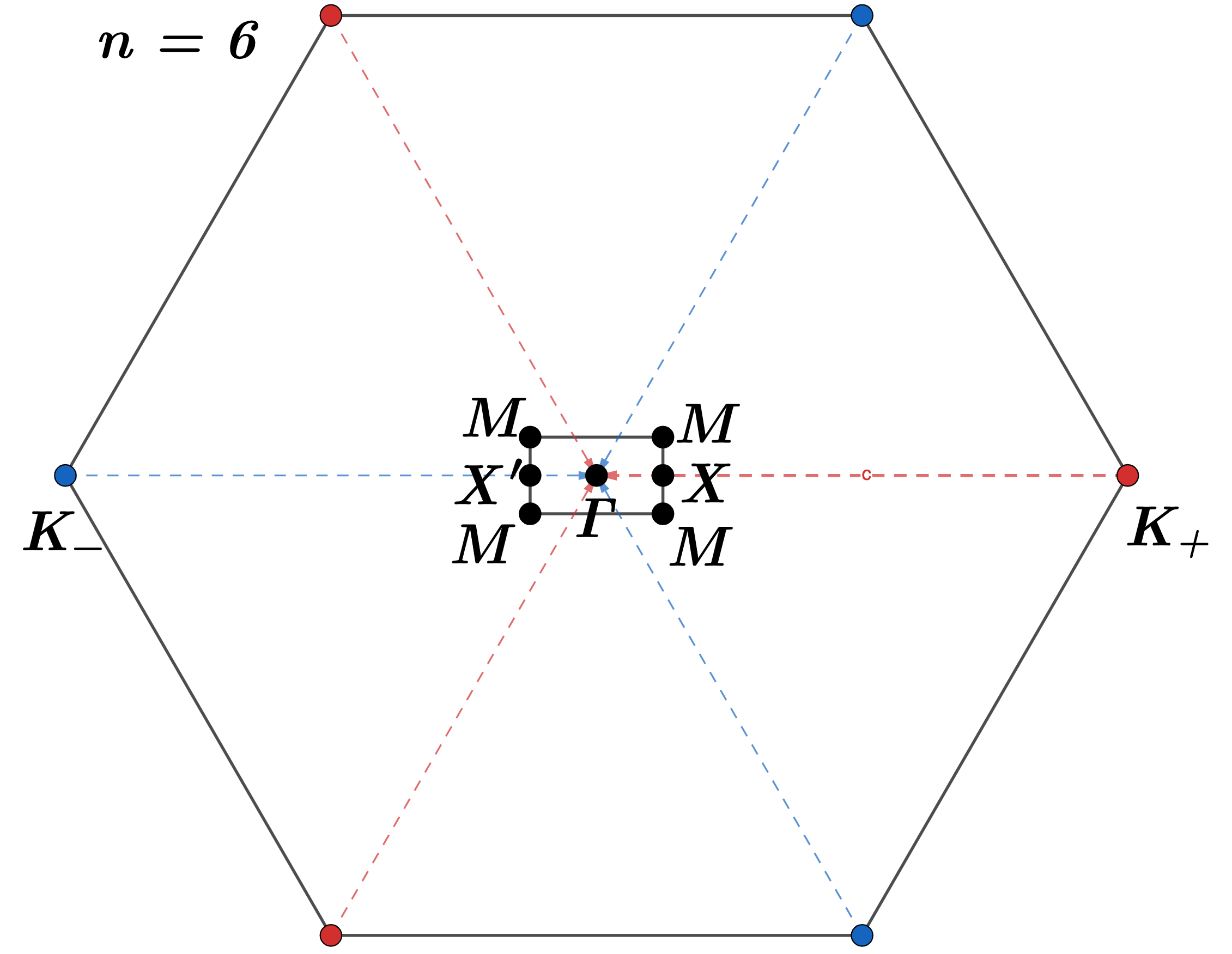
Therefore, folds onto the point , i.e., along to or to path and its corresponding valley pseudospin and showing the periodicity of through the index, and is independent of the size index or hole radii . Fig. 6) presents such folding sequence from to .
It is noteworthy that when , folds to the point, leading to valley degeneracy. Upon introducing holes in graphene (without dangling bonds), sublattice and inversion symmetries are broken, resulting in gaps at the Dirac points for [79, 80, 81, 82, 83, 84]. However, is a point protected by other symmetries, ensuring the preservation of the two degenerate cones when . To induce a gap at , dangling bonds are necessary, which breaks bond symmetry [85, 86].
Therefore, the imbalance density, the folding of the Brillouin zone, and symmetry breaking explain the behavior of the gap size shown in Fig. 5.
a)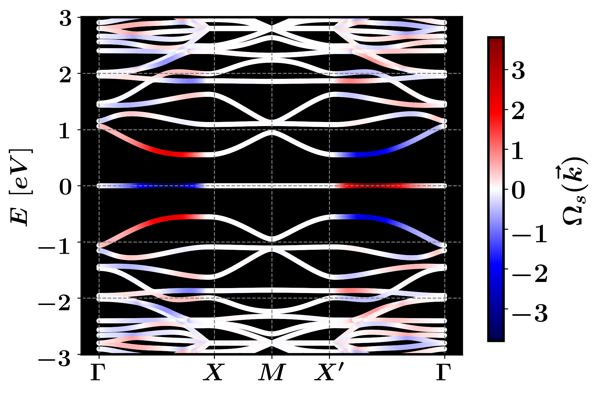 b)
b) 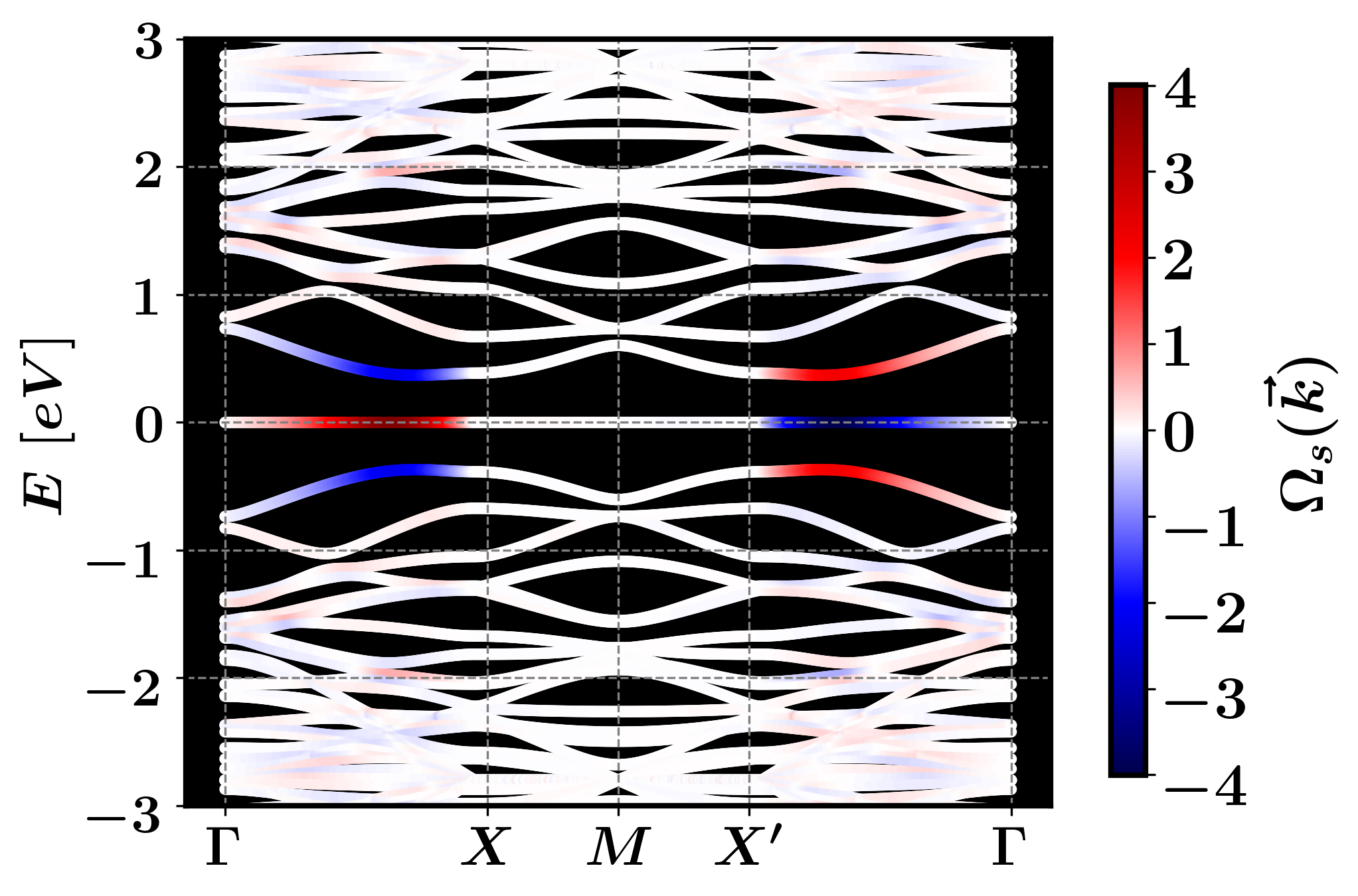
c) 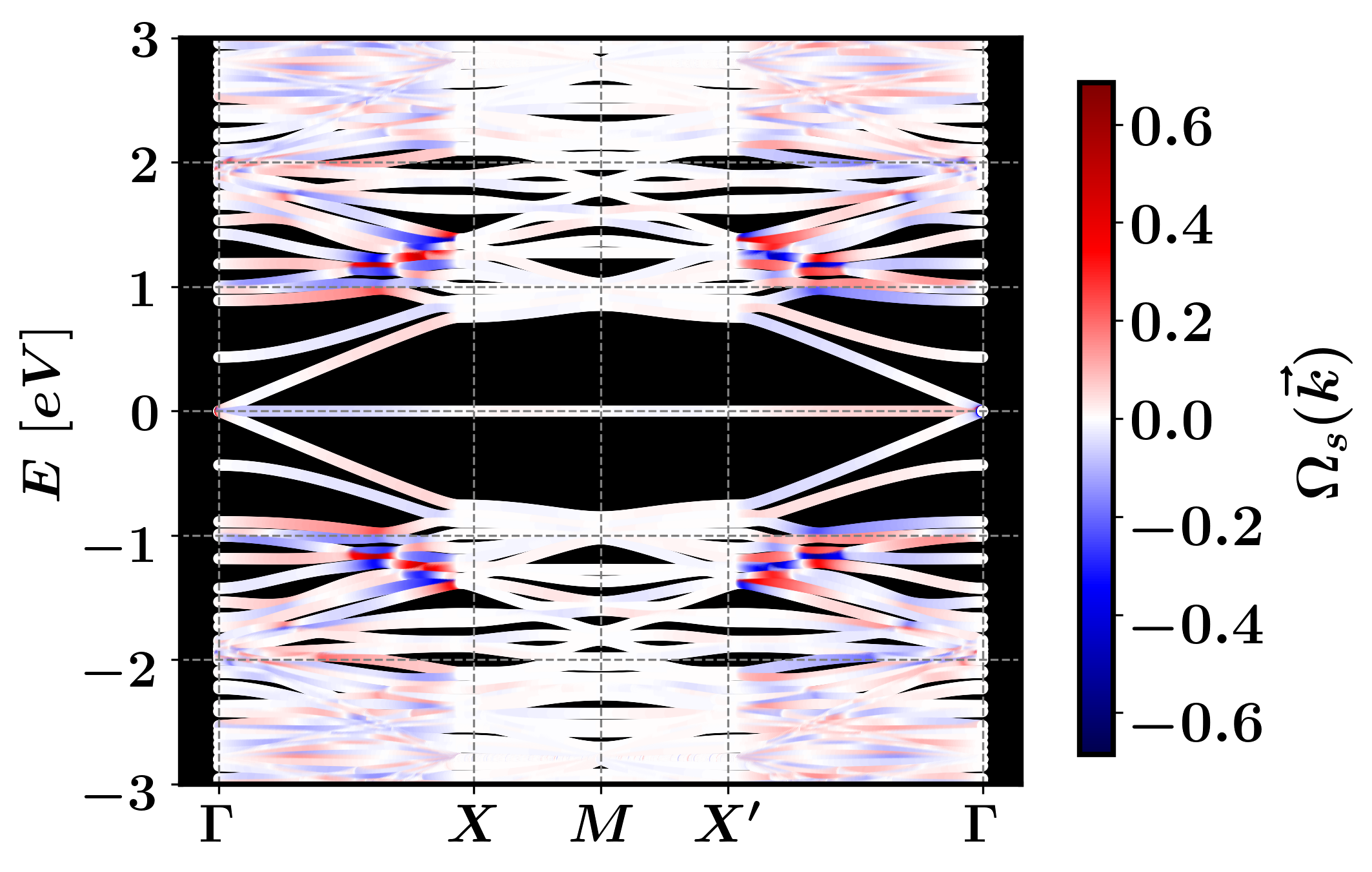 d)
d) 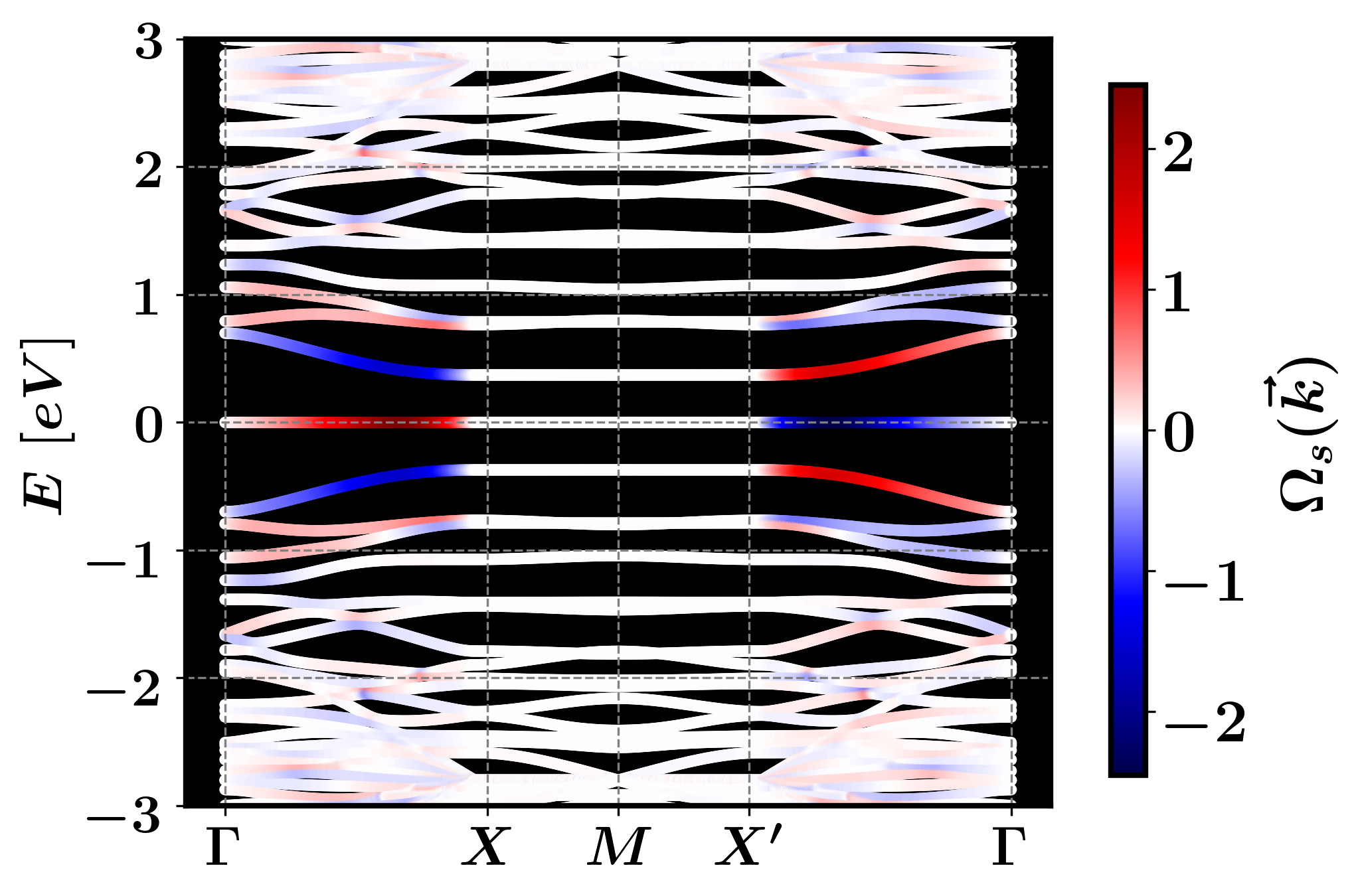
e) 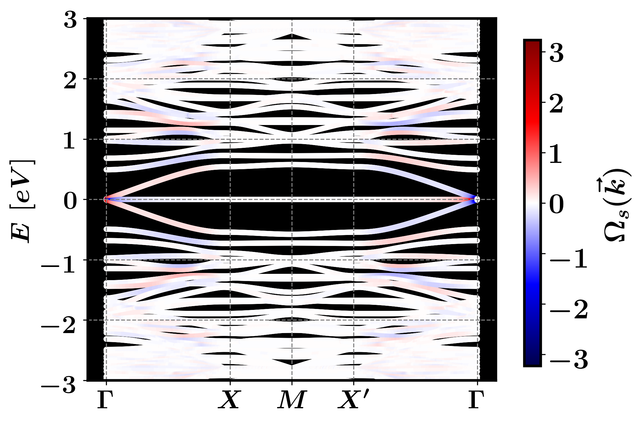 f)
f) 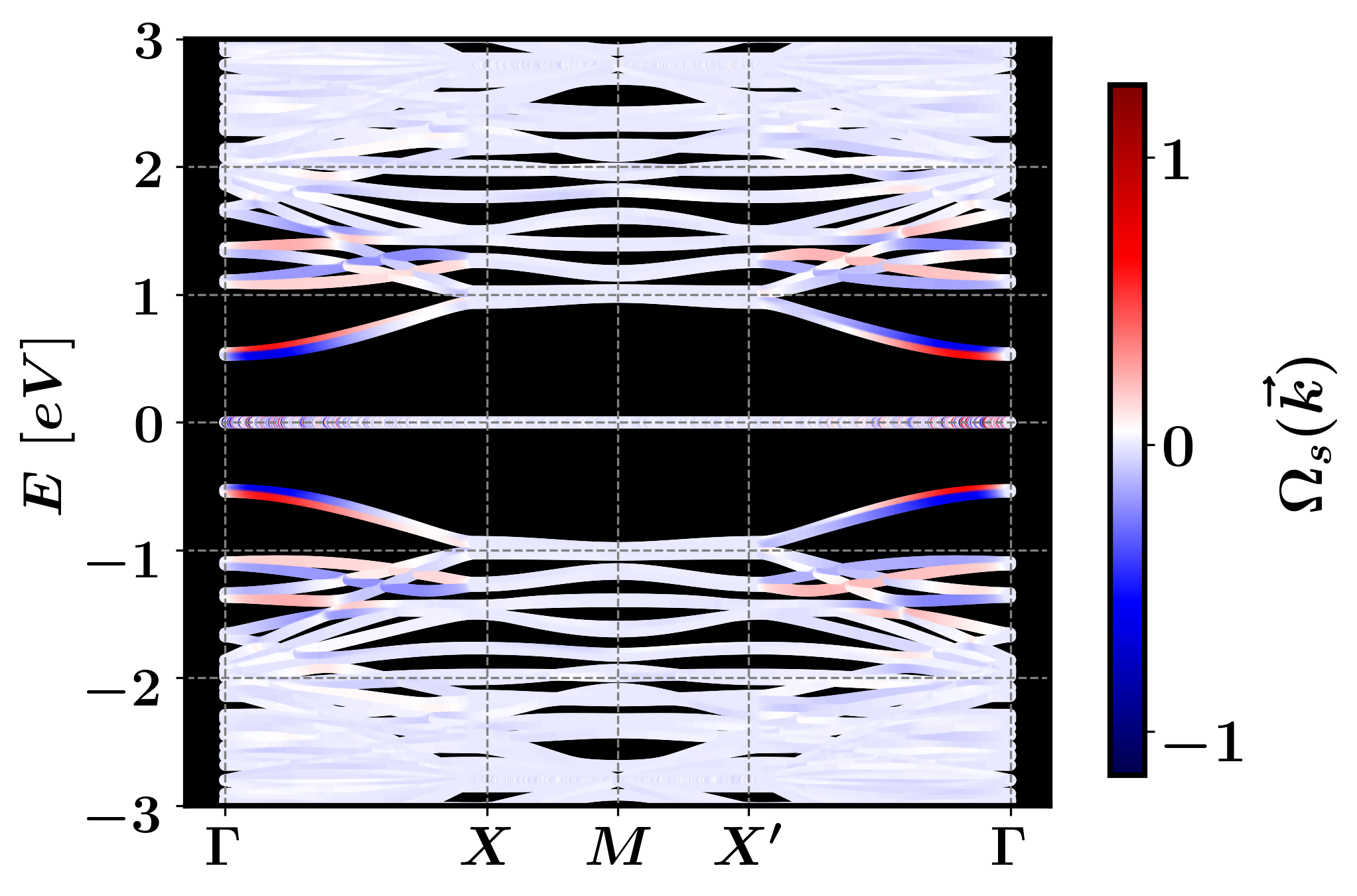
Additionally, Fig. 7 shows the Berry curvature for the unit cells shown in Fig. 2 as a function of and the band . The Berry curvature is denoted as and defined as,
| (8) |
where is the Berry connection and are the periodic functions in the Bloch states that solve the Schrödinger equation. Figure Fig. 7 illustrates how the symmetry breaking induces a nonzero Berry curvature at the folding points and in the vicinity of .
Finally, near the high-symmetry points of the reciprocal folded lattice and without dangling bond three symmetric bands around are formed, one for valence, the flat band, and the conduction band, denoted by , respectively. Folding the Dirac points at would, in principle, yield two bands with linear dispersion and a flat band at . Therefore, an appropriate Hamiltonian for this description is the model [87], defined by
| (9) |
where with a parameter, and , and are the pseudospin operators and Fermi velocity, respectively; given by
| (13) | |||
| (17) |
with , and a constant that depends on unit cell size and hole size . Such hamiltonian is the most simple one that has flat bands and under electromagnetic radiation, behaves as a two- or three-level Rabi system with clear optical signatures of flat bands [87].
As discussed previously, breaking inversion and sublattice symmetry results in the opening of a gap. Therefore, the low-energy Hamiltonian around will exhibit an additional mass-like term to the Hamiltonian, thus the low-energy hamiltonian is
| (18) |
where is a pseudospin operator defined as
| (19) |
and is the mass-like term that depends on and pseudospin index . It can be constructed from the expansion of energies for the bands , given by
| (20) | |||||
where can be numerically determined. Then is expressed as,
| (21) |
In Fig. 8, the electronic bands obtained from the Hamiltonian (dashed black, blue and red lines) and the low-energy approximation with the Hamiltonian (Eq. 18) (solid black, blue and red lines) are depicted. In general a excellent agreement is obtained.
a)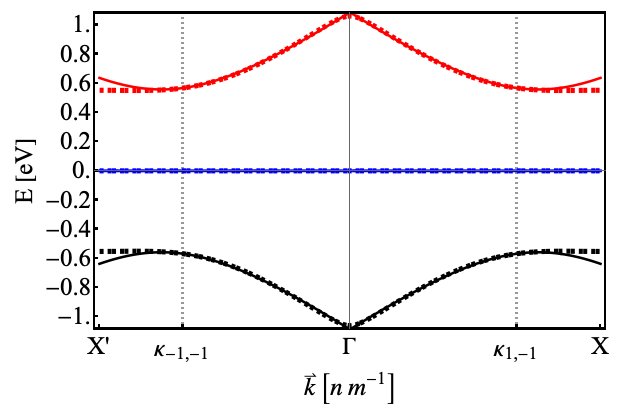 b)
b) 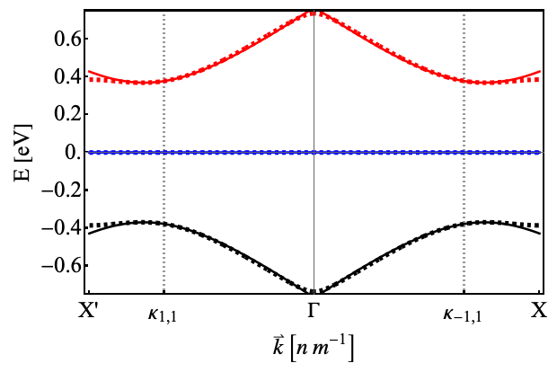
c) 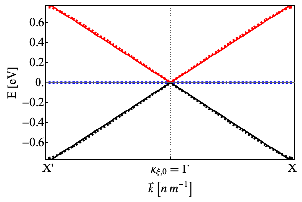 d)
d) 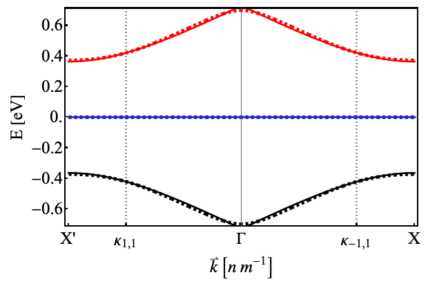
e) 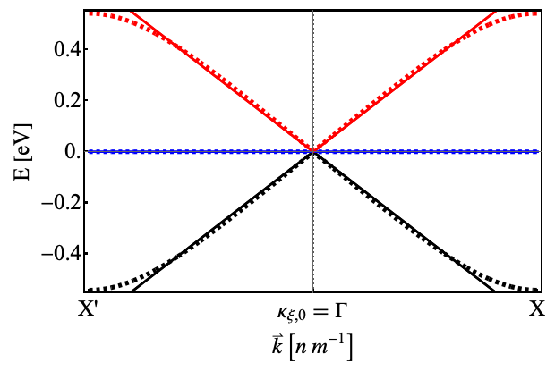
4 Concluding remarks
In this paper, we investigated the formation of flat bands in two-dimensional periodic holey graphene (2D HG). Our findings reveal that these flat band states exhibit significantly higher localization when compared to other states, particularly in the zigzag edge regions surrounding the hole. This highlights a connection between flat band formation and Compact Localized States (CLS), as investigated in prior works [70, 71, 10]. Moreover, we establish that sublattice site imbalance, achieved through the breaking of path-exchange symmetry [76, 10], induces the formation of flat bands, while the breaking of sublattice and inversion symmetry leads to the creation of energy gaps.
Furthermore, we have discussed the influence of unit cell size and hole dimensions on the gap size and density of states (DOS) at , through the imbalance density . Additionally, we have explored the existence of semimetallicity in 2D HG with a periodicity of , arising from the folding of points to the point, protected by bond symmetry, except when introducing dangling bonds that break this symmetry, resulting in a gap. We demonstrated that the breaking of the discussed symmetries (inversion, sublattice, and bond) generates a non-zero Berry curvature.
Finally, we establish a continuous Hamiltonian model for three bands in cases where the hole radius and there are no dangling bonds. This model consists of an type Hamiltonian and a mass-like term that opens the gap at points.
Our work gives a protocol that allows to obtain flat bands at will and thus gives a possible new 2D material to obtain highly correlated quantum phases without twists.
Acknowledgements
This work was supported by CONAHCyT project 1564464 and UNAM DGAPA project IN101924. Abdiel de Jesús Espinosa-Champo is supported by a CONAHCyT PhD fellowship (No. CVU 1007044). The authors acknowledge and express gratitude to Carlos Ernesto López Natarén from Secretaria Técnica de Cómputo y Telecomunicaciones for his valuable support.
References
References
- [1] Qiu W X, Li S, Gao J H, Zhou Y and Zhang F C 2016 Phys. Rev. B 94(24) 241409 URL https://link.aps.org/doi/10.1103/PhysRevB.94.241409
- [2] Drost R, Ojanen T, Harju A and Liljeroth P 2017 Nature Physics 13 668–671 ISSN 1745-2481
- [3] Abilio C C, Butaud P, Fournier T, Pannetier B, Vidal J, Tedesco S and Dalzotto B 1999 Phys. Rev. Lett. 83(24) 5102–5105 URL https://link.aps.org/doi/10.1103/PhysRevLett.83.5102
- [4] Taie S, Ozawa H, Ichinose T, Nishio T, Nakajima S and Takahashi Y 2015 Science Advances 1 e1500854 (Preprint https://www.science.org/doi/pdf/10.1126/sciadv.1500854) URL https://www.science.org/doi/abs/10.1126/sciadv.1500854
- [5] Nakata Y, Okada T, Nakanishi T and Kitano M 2012 Phys. Rev. B 85(20) 205128 URL https://link.aps.org/doi/10.1103/PhysRevB.85.205128
- [6] He Y, Mao R, Cai H, Zhang J X, Li Y, Yuan L, Zhu S Y and Wang D W 2021 Physical Review Letters 126 103601 ISSN 0031-9007, 1079-7114
- [7] Cao Y, Fatemi V, Fang S, Watanabe K, Taniguchi T, Kaxiras E and Jarillo-Herrero P 2018 Nature 556 43–50 URL https://doi.org/10.1038/nature26160
- [8] Naumis G G, Navarro-Labastida L A, Aguilar-Méndez E and Espinosa-Champo A 2021 Phys. Rev. B 103(24) 245418 URL https://link.aps.org/doi/10.1103/PhysRevB.103.245418
- [9] Navarro-Labastida L A, Espinosa-Champo A, Aguilar-Mendez E and Naumis G G 2022 Phys. Rev. B 105(11) 115434 URL https://link.aps.org/doi/10.1103/PhysRevB.105.115434
- [10] de Jesús Espinosa-Champo A and Naumis G G 2023 Journal of Physics: Condensed Matter 36 015502 URL https://dx.doi.org/10.1088/1361-648X/acfbd1
- [11] Bergholtz E J and Liu Z 2013 International Journal of Modern Physics B 27 1330017 ISSN 0217-9792, 1793-6578
- [12] Nguyen H S, Dubois F, Deschamps T, Cueff S, Pardon A, Leclercq J L, Seassal C, Letartre X and Viktorovitch P 2018 Phys. Rev. Lett. 120(6) 066102 URL https://link.aps.org/doi/10.1103/PhysRevLett.120.066102
- [13] Deng S, Simon A and Köhler J 2003 Journal of Solid State Chemistry 176 412–416 ISSN 0022-4596 special issue on The Impact of Theoretical Methods on Solid-State Chemistry URL https://www.sciencedirect.com/science/article/pii/S0022459603002391
- [14] Mielke A and Tasaki H 1993 Communications in Mathematical Physics 158 341–371 ISSN 1432-0916
- [15] Tasaki H 1998 Progress of Theoretical Physics 99 489–548 ISSN 0033-068X
- [16] Aoki H 2020 Journal of Superconductivity and Novel Magnetism 33 2341–2346 URL https://doi.org/10.1007/s10948-020-05474-6
- [17] Wu C, Bergman D, Balents L and Das Sarma S 2007 Phys. Rev. Lett. 99(7) 070401 URL https://link.aps.org/doi/10.1103/PhysRevLett.99.070401
- [18] Jaworowski B, Güçlü A D, Kaczmarkiewicz P, Kupczyński M, Potasz P and Wójs A 2018 New Journal of Physics 20 063023 URL https://dx.doi.org/10.1088/1367-2630/aac690
- [19] Navarro-Labastida L A and Naumis G G 2023 Phys. Rev. B 107(15) 155428 URL https://link.aps.org/doi/10.1103/PhysRevB.107.155428
- [20] Navarro Labastida L A and G Naumis G 2023 Revista Mexicana de Física 69 041602 1– URL https://rmf.smf.mx/ojs/index.php/rmf/article/view/6795
- [21] Roman-Taboada P and Naumis G G 2017 Phys. Rev. B 95(11) 115440 URL https://link.aps.org/doi/10.1103/PhysRevB.95.115440
- [22] Roman-Taboada P and Naumis G G 2017 Phys. Rev. B 96(15) 155435 URL https://link.aps.org/doi/10.1103/PhysRevB.96.155435
- [23] Roman-Taboada P and Naumis G G 2017 Journal of Physics Communications 1 055023 URL https://dx.doi.org/10.1088/2399-6528/aa98fd
- [24] Mao J, Milovanović S P, Anđelković M, Lai X, Cao Y, Watanabe K, Taniguchi T, Covaci L, Peeters F M, Geim A K, Jiang Y and Andrei E Y 2020 Nature 584 215–220 URL https://doi.org/10.1038/s41586-020-2567-3
- [25] Manesco A L R and Lado J L 2021 2D Materials 8 035057 URL https://dx.doi.org/10.1088/2053-1583/ac0b48
- [26] Manesco A L R, Lado J L, Ribeiro E V S, Weber G and Jr D R 2020 2D Materials 8 015011 URL https://dx.doi.org/10.1088/2053-1583/abbc5f
- [27] Milovanović S P, Anđelković M, Covaci L and Peeters F M 2020 Phys. Rev. B 102(24) 245427 URL https://link.aps.org/doi/10.1103/PhysRevB.102.245427
- [28] Mahmud M T, Zhai D and Sandler N 2023 Nano Letters 23 7725–7732 pMID: 37578461 (Preprint https://doi.org/10.1021/acs.nanolett.3c02513) URL https://doi.org/10.1021/acs.nanolett.3c02513
- [29] Andrade E, López-Urías F and Naumis G G 2023 Phys. Rev. B 107(23) 235143 URL https://link.aps.org/doi/10.1103/PhysRevB.107.235143
- [30] Gonzalez-Arraga L A, Lado J L, Guinea F and San-Jose P 2017 Phys. Rev. Lett. 119(10) 107201 URL https://link.aps.org/doi/10.1103/PhysRevLett.119.107201
- [31] Carr S, Fang S, Jarillo-Herrero P and Kaxiras E 2018 Phys. Rev. B 98(8) 085144 URL https://link.aps.org/doi/10.1103/PhysRevB.98.085144
- [32] Yndurain F 2019 Phys. Rev. B 99(4) 045423 URL https://link.aps.org/doi/10.1103/PhysRevB.99.045423
- [33] Wu Z, Kuang X, Zhan Z and Yuan S 2021 Phys. Rev. B 104(20) 205104 URL https://link.aps.org/doi/10.1103/PhysRevB.104.205104
- [34] Sánchez-Ochoa F, Rubio-Ponce A and López-Urías F 2023 Phys. Rev. B 107(4) 045414 URL https://link.aps.org/doi/10.1103/PhysRevB.107.045414
- [35] You J Y, Gu B and Su G 2019 Scientific Reports 9 20116 ISSN 2045-2322 URL https://doi.org/10.1038/s41598-019-56738-8
- [36] Sedelnikova O V, Stolyarova S G, Chuvilin A L, Okotrub A V and Bulusheva L G 2019 Applied Physics Letters 114 091901 ISSN 0003-6951 (Preprint https://pubs.aip.org/aip/apl/article-pdf/doi/10.1063/1.5080617/13495677/091901_1_online.pdf) URL https://doi.org/10.1063/1.5080617
- [37] Mahmood J, Lee E K, Jung M, Shin D, Jeon I Y, Jung S M, Choi H J, Seo J M, Bae S Y, Sohn S D, Park N, Oh J H, Shin H J and Baek J B 2015 Nature Communications 6 6486 URL https://doi.org/10.1038/ncomms7486
- [38] Zhao Y, Dai Z, Lian C and Meng, S 2017 RSC Adv. 7(42) 25803–25810 URL http://dx.doi.org/10.1039/C7RA03597G
- [39] Omidvar A 2017 Materials Chemistry and Physics 202 258–265 ISSN 0254-0584 URL https://www.sciencedirect.com/science/article/pii/S0254058417307290
- [40] de Sousa M S M, Liu F, Qu F and Chen W 2022 Phys. Rev. B 105(1) 014511 URL https://link.aps.org/doi/10.1103/PhysRevB.105.014511
- [41] Yang J, Ma M, Li L, Zhang Y, Huang W and Dong X 2014 Nanoscale 6 13301–13313 URL http://dx.doi.org/10.1039/C4NR04584J
- [42] Lin Y, Liao Y, Chen Z and Connell J W 2017 Materials Research Letters 5 209–234 URL https://doi.org/10.1080/21663831.2016.1271047
- [43] Liu X, Cho S M, Lin S, Chen Z, Choi W, Kim Y M, Yun E, Baek E H, Ryu D H and Lee H 2022 Matter 5 2306–2318 URL https://doi.org/10.1016/j.matt.2022.04.033
- [44] Naumis G G 2007 Phys. Rev. B 76(15) 153403 URL https://link.aps.org/doi/10.1103/PhysRevB.76.153403
- [45] Xu K, Urgel J, Eimre K, Di Giovannantonio M, Keerthi A, Komber H, Wang S, Narita A, Berger R, Ruffieux P, Pignedoli C A, Liu J, Müllen K, Fasel R and Feng X 2019 Journal of the American Chemical Society 141 7726–7730 URL https://doi.org/10.1021/jacs.9b03554
- [46] Singh D, Shukla V and Ahuja R 2020 Phys. Rev. B 102(7) 075444 URL https://link.aps.org/doi/10.1103/PhysRevB.102.075444
- [47] Rajput N S, Al Zadjali S, Gutierrez M, Esawi A M K and Al Teneiji M 2021 RSC Advances 11 27381–27405 URL http://dx.doi.org/10.1039/D1RA05157A
- [48] Lokhande A C, Qattan I A, Lokhande C D and Patole S P 2020 Journal of Materials Chemistry A 8 918–977 URL http://dx.doi.org/10.1039/C9TA10667G
- [49] Plaza-Rivera C O, Viggiano R P, Dornbusch D A, Wu J J, Connell J W and Lin Y 2021 Frontiers in Energy Research 9 ISSN 2296-598X URL https://www.frontiersin.org/articles/10.3389/fenrg.2021.703676
- [50] Liu T, Zhang L, Cheng B, Hu X and Yu J 2020 Cell Reports Physical Science 1 URL https://doi.org/10.1016/j.xcrp.2020.100215
- [51] Lin Y, Liao Y, Chen Z and Connell J W 2017 Materials Research Letters 5 209–234 (Preprint https://doi.org/10.1080/21663831.2016.1271047) URL https://doi.org/10.1080/21663831.2016.1271047
- [52] Barkov P V and Glukhova O E 2021 Nanomaterials 11 1074 ISSN 2079-4991 URL http://dx.doi.org/10.3390/nano11051074
- [53] Fischbein M D and Drndić M 2008 Applied Physics Letters 93 113107 ISSN 0003-6951 (Preprint https://pubs.aip.org/aip/apl/article-pdf/doi/10.1063/1.2980518/14401035/113107_1_online.pdf) URL https://doi.org/10.1063/1.2980518
- [54] Khan K, Liu T, Arif M, Yan X, Hossain M D, Rehman F, Zhou S, Yang J, Sun C, Bae S H, Kim J, Amine K, Pan X and Luo Z 2021 Advanced Energy Materials 11 2101619 (Preprint %****␣Flat_bands_without_twist_holey_graphene.tex␣Line␣650␣****https://onlinelibrary-wiley-com.pbidi.unam.mx:2443/doi/pdf/10.1002/aenm.202101619) URL https://onlinelibrary-wiley-com.pbidi.unam.mx:2443/doi/abs/10.1002/aenm.202101619
- [55] Kazemizadeh F and Malekfar R 2018 Physica B: Condensed Matter 530 236–241 ISSN 0921-4526 URL https://www.sciencedirect.com/science/article/pii/S092145261730947X
- [56] Wang F, Mei X, Wang K, Dong X, Gao M, Zhai Z, Lv J, Zhu C, Duan W and Wang W 2019 Journal of Materials Science 54 5658–5670 URL https://doi.org/10.1007/s10853-018-03247-0
- [57] Lin J, Peng Z, Liu Y, Ruiz-Zepeda F, Ye R, Samuel E L G, Yacaman M J, Yakobson B I and Tour J M 2014 Nature Communications 5 5714 URL https://doi.org/10.1038/ncomms6714
- [58] Kumar R, Pérez del Pino A, Sahoo S, Singh R K, Tan W K, Kar K K, Matsuda A and Joanni E 2022 Progress in Energy and Combustion Science 91 100981 ISSN 0360-1285 URL https://www.sciencedirect.com/science/article/pii/S0360128521000794
- [59] Joshi P, Shukla S, Gupta S, Riley P R, Narayan J and Narayan R 2022 ACS Applied Materials & Interfaces 14 37149–37160 URL https://doi.org/10.1021/acsami.2c09096
- [60] Haruyama J 2013 Electronics 2 368–386 ISSN 2079-9292 URL http://dx.doi.org/10.3390/electronics2040368
- [61] Lin Y, Plaza-Rivera C O, Hu L and Connell J W 2022 Accounts of Chemical Research 55 3020–3031 pMID: 36173244 (Preprint https://doi.org/10.1021/acs.accounts.2c00457) URL https://doi.org/10.1021/acs.accounts.2c00457
- [62] Zhang Y, Wan Q and Yang N 2019 Small 15 1903780 (Preprint https://onlinelibrary-wiley-com.pbidi.unam.mx:2443/doi/pdf/10.1002/smll.201903780) URL https://onlinelibrary-wiley-com.pbidi.unam.mx:2443/doi/abs/10.1002/smll.201903780
- [63] White D L, Lystrom L, He X, Burkert S C, Kilin D S, Kilina S and Star A 2020 ACS Applied Materials & Interfaces 12 36513–36522 URL https://doi.org/10.1021/acsami.0c09394
- [64] Zhang J, Song H, Zeng D, Wang H, Qin Z, Xu K, Pang A and Xie C 2016 Scientific Reports 6 32310 URL https://doi.org/10.1038/srep32310
- [65] Bai J, Zhong X, Jiang S, Huang Y and Duan X 2010 Nature Nanotechnology 5 190–194 URL https://doi.org/10.1038/nnano.2010.8
- [66] Moldovan D, Anłdelković M and Peeters F 2020 pybinding v0.9.5: a Python package for tight- binding calculations This work was supported by the Flemish Science Foundation (FWO-Vl) and the Methusalem Funding of the Flemish Government. URL https://doi.org/10.5281/zenodo.4010216
- [67] Lado J L 2021 GitHub - joselado/pyqula: Python library to compute different properties of quantum tight binding models in a lattice. https://github.com/joselado/pyqula
- [68] Li Y, Zhan Z, Kuang X, Li Y and Yuan S 2023 Computer Physics Communications 285 108632 ISSN 0010-4655 URL https://www.sciencedirect.com/science/article/pii/S0010465522003514
- [69] Koh K H, Bagherzadeh Mostaghimi A H, Chang Q, Kim Y J, Siahrostami S, Han T H and Chen Z 2023 EcoMat 5 e12266 (Preprint https://onlinelibrary-wiley-com.pbidi.unam.mx:2443/doi/pdf/10.1002/eom2.12266) URL https://onlinelibrary-wiley-com.pbidi.unam.mx:2443/doi/abs/10.1002/eom2.12266
- [70] Naumis G G, Barrio R A and Wang C 1994 Phys. Rev. B 50(14) 9834–9842 URL https://link.aps.org/doi/10.1103/PhysRevB.50.9834
- [71] Naumis G G, Wang C and Barrio R A 2002 Phys. Rev. B 65(13) 134203 URL https://link.aps.org/doi/10.1103/PhysRevB.65.134203
- [72] Bell R J and Dean P 1970 Discuss. Faraday Soc. 50(0) 55–61 URL http://dx.doi.org/10.1039/DF9705000055
- [73] Edwards J T and Thouless D J 1972 Journal of Physics C: Solid State Physics 5 807 URL https://dx.doi.org/10.1088/0022-3719/5/8/007
- [74] Shukla P 2018 Phys. Rev. B 98(5) 054206 URL https://link.aps.org/doi/10.1103/PhysRevB.98.054206
- [75] Wegner F 1980 Zeitschrift für Physik B Condensed Matter 36 209–214 URL https://doi.org/10.1007/BF01325284
- [76] Bae J H, Sedrakyan T and Maiti S 2023 SciPost Phys. 15 139 URL https://scipost.org/10.21468/SciPostPhys.15.4.139
- [77] Naumis G G and Roman-Taboada P 2014 Phys. Rev. B 89(24) 241404 URL https://link.aps.org/doi/10.1103/PhysRevB.89.241404
- [78] Barrios-Vargas J and Naumis G G 2013 Solid State Communications 162 23–27 ISSN 0038-1098 URL https://www.sciencedirect.com/science/article/pii/S0038109813001221
- [79] Wang E, Lu X, Ding S, Yao W, Yan M, Wan G, Deng K, Wang S, Chen G, Ma L, Jung J, Fedorov A V, Zhang Y, Zhang G and Zhou S 2016 Nature Physics 12 1111–1115 ISSN 1745-2481 URL https://doi.org/10.1038/nphys3856
- [80] Kou L, Hu F, Yan B, Frauenheim T and Chen C 2014 Nanoscale 6(13) 7474–7479 URL http://dx.doi.org/10.1039/C4NR01102C
- [81] Nishidate K, Matsukawa M and Hasegawa M 2023 Surface Science 728 122196 ISSN 0039-6028 URL https://www.sciencedirect.com/science/article/pii/S0039602822001819
- [82] Agrawal B and Agrawal S 2013 Physica E: Low-dimensional Systems and Nanostructures 50 102–107 ISSN 1386-9477 URL https://www.sciencedirect.com/science/article/pii/S1386947713000684
- [83] Malterre D, Kierren B, Fagot-Revurat Y, Didiot C, de Abajo F J G, Schiller F, Cordón J and Ortega J E 2011 New Journal of Physics 13 013026 URL https://dx.doi.org/10.1088/1367-2630/13/1/013026
- [84] Zhou S Y, Gweon G H, Fedorov A V, First P N, de Heer W A, Lee D H, Guinea F, Castro Neto A H and Lanzara A 2007 Nature Materials 6 770–775 ISSN 1476-4660 URL https://doi.org/10.1038/nmat2003
- [85] Jia T T, Fan X Y, Zheng M M and Chen G 2016 Scientific Reports 6 20971 ISSN 2045-2322 URL https://doi.org/10.1038/srep20971
- [86] Ye M, Quhe R, Zheng J, Ni Z, Wang Y, Yuan Y, Tse G, Shi J, Gao Z and Lu J 2014 Physica E: Low-dimensional Systems and Nanostructures 59 60–65 ISSN 1386-9477 URL https://www.sciencedirect.com/science/article/pii/S1386947713004530
- [87] Mojarro M A, Ibarra-Sierra V G, Sandoval-Santana J C, Carrillo-Bastos R and Naumis G G 2020 Phys. Rev. B 101(16) 165305 URL https://link.aps.org/doi/10.1103/PhysRevB.101.165305