Scaling Is All You Need: Autonomous Driving with JAX-Accelerated Reinforcement Learning

Abstract

Reinforcement learning has been demonstrated to outperform even the best humans in complex domains like video games. However, running reinforcement learning experiments on the required scale for autonomous driving is extremely difficult. Building a large scale reinforcement learning system and distributing it across many GPUs is challenging. Gathering experience during training on real world vehicles is prohibitive from a safety and scalability perspective. Therefore, an efficient and realistic driving simulator is required that uses a large amount of data from real-world driving. We bring these capabilities together and conduct large-scale reinforcement learning experiments for autonomous driving. We demonstrate that our policy performance improves with increasing scale. Our best performing policy reduces the failure rate by 64% while improving the rate of driving progress by 25% compared to the policies produced by state-of-the-art machine learning for autonomous driving.

1 Introduction

We want to develop an autonomous driving planning system that is safer than human drivers, to be deployed on real-world vehicles on a large scale. Prior work has outperformed even the best humans in other complex domains such as video games (Berner et al., 2019; Vinyals et al., 2019) using reinforcement learning (RL) methods. These results found that scaling RL methods to large distributed settings that learn across hundreds of GPUs over multiple month and therefore on massive amounts of simulation data was key to finding the best policies.

However, it is challenging to apply this lesson of scaling the training process to autonomous driving. This real-world problem introduces additional challenges compared to the video game setting. For video games, the original game environment can be used to gather experience during RL training. This in situ training is relatively cheap and does not carry real-world risk. Running RL policies during training on real-world vehicles is inconceivable — reinforcement learning would require the experience of negative examples such as crashes with other vehicles and pedestrians, and the costs of operating a sufficiently large fleet of vehicles in the real world would be prohibitive. Therefore, effective RL for driving requires building an efficient and realistic autonomous driving simulator.

Recent work (Gulino et al., 2023) focused on such a simulator. It uses recorded data from human-operated vehicles in the real world to simulate traffic scenes realistically and allows one or many agents in the scene to be controlled. But the work finds that training an RL agent against reactive agents is less effective than training against logged agents. Other work that combines behavioral cloning (BC) with RL to train policies for autonomous driving (Lu et al., 2023) also uses logged agents to train and evaluate the policies. However, using logged agents limits the diversity of agent interactions and therefore the state space of the simulation. This is a distinct difference to other RL settings, in which the goal environment generates diverse interactions that allow exploration of the entire state space.

In this paper, we set up a scalable reinforcement learning framework and combine it with an efficient simulator for autonomous driving based on real-world data. We then conduct experiments on billions of agent steps with different model sizes in order to determine if we can overcome the constrained state space of the simulator by using increasingly more real-world data.

The main contributions of our work are:

1. We demonstrate how to use prerecorded real-world driving data in a hardware-accelerated simulator as part of distributed reinforcement learning to achieve improving policy performance with increasing experiment size.

2. We demonstrate that our largest scale experiments, using a 25M parameter model on 6000 h of human-expert driving from San Francisco training on 2.5 billion agent steps, reduced the failure rate compared to the current state of the art (Lu et al., 2023) by 64%.

These contributions emphasize the importance of efficient, accurate and scalable simulation for real-world reinforcement learning.

2 Related work

In this paper we present a hardware-accelerated autonomous driving simulator for real-world driving scenarios, which is similar to Waymax (Gulino et al., 2023). Waymax also trains RL agents but only reported results from 30 million agent steps, approximately two orders of magnitude less than our experiments. Nocturne (Vinitsky et al., 2023) and MetaDrive (Li et al., 2022) are two examples of autonomous driving simulators not specifically designed for accelerated hardware but with similar features and using real-world data. The Carla simulator (Dosovitskiy et al., 2017), based on synthetic scenarios, has been used across different publications to compare the performance of driving algorithms, but not at the scale of results we report here.

Training highly performant policies in complex and continuous real-world domains has mainly been achieved with distributed and scalable reinforcement learning using actor-critic methods. However, most existing results focus not on real-world problems but on video game environments (Vinyals et al., 2019; Berner et al., 2019).

Of the techniques that have been used to train autonomous driving policies, the closest to our work is Imitation Is Not Enough (Lu et al., 2023) which also uses a combination of imitation learning (IL) and RL to train strong driving policies on a large dataset of real-world driving scenarios. That work established two fundamental driving metrics (failure rate and progress ratio) and provides a detailed description of the mining process of their evaluation dataset. The presented policies are state of the art (SOTA) and we will compare our best policy to theirs. However, no scalable distributed RL system has been presented, and the scale of the conducted reinforcement learning experiments remains unclear. Other work focuses on realistic traffic simulation (Zhang et al., 2023), but also trains policies with a combined IL and RL approach. However, their datasets are approximately 3 orders of magnitude smaller than ours and focus on highway driving, which does not pose as complex challenges as the dense urban driving we focus on. Imitation learning approaches in open loop (Bronstein et al., 2022b; Zhang et al., 2021; Vitelli et al., 2021) and closed loop (Bronstein et al., 2022a; Igl et al., 2022) have also been proposed for autonomous driving. As Lu et al. (2023) argue, IL approaches lack explicit knowledge of unsafe driving and can respond inappropriate in rare, long tail scenarios.

3 Large scale RL for autonomous driving

The challenges of using large scale reinforcement learning for autonomous driving are manifold. To achieve scale, the real-world problem must be modeled by a simulator, which requires creating realistic traffic scenes and modeling the interactions between different dynamic agents. The simulator must be sufficiently efficient to generate environment interactions on the order of billions of steps in reasonable time and computational cost. Finally, a distributed learning architecture must be identified that can learn efficiently and scalably. Learners and simulation actors must be created across many machines, each leveraging parallel hardware, i.e. GPUs.

3.1 Scene generation and agent interactions

There are different ways of creating traffic scenes for simulation. Simulations scenarios can be generated entirely synthetically, including the placement of roads, agents, and traffic signals, for example as in the Carla simulator (Dosovitskiy et al., 2017). While entirely synthetic simulation gives very fine grained control over training scenario distribution, this approach raises the challenge of identifying what that scenario distribution should be, and how best to sample training instances from it. A different approach is to create scenes based on real-world data recorded from vehicles equipped with sensors, such as cameras and lidar sensors, driving on public roads. From the recorded sensor data, a 3D-scene can be created that contains, for example, the observed traffic light states and challenging obstacles, such as pedestrians, cyclists, and cars (Gulino et al., 2023). In this work, we use scenarios that have been created from real-world driving, for the fidelity of their representation of the real world.

For simulating driving scenarios, a critical question is how to simulate the behavior of other agents in a realistic manner, especially in response to the learning agent’s own behavior. Existing approaches implemented control policies for synthetic agents that are reactive in response to the behavior of other agents including the learning agent. However, constructing these reactive policies, especially for diverse entities such as bikes and pedestrians, is arguably as hard as the original learning problem. Furthermore, it is unclear if and how such reactive agents help training reinforcement policies — Waymax (Gulino et al., 2023) found that using reactive agents impaired the performance of learner policy, possibly as a result of the learner exploiting the agents’ reactiveness.

To address these challenges, we use the recorded behavior of real-world agents in our simulations. This approach creates its own challenges in that the other agents will not respond to the learning agent’s behavior. This creates the phenomenon of “simulation divergence” where the other agent’s behavior no longer resembles what would actually happen, e.g., following agents might cause rear-end collisions in response to the learning agent slowing down, although in reality the following agents would slow down too. Additionally, the number and diversity of interactions with other agents is limited by the amount of real-world data used to create the traffic scenes, which is a particular challenge when learning behavior in very rare but critical settings.

Despite these challenges, our experience was that logged data was far more representative of agent behavior than could be implemented synthetically. Lack of realism due to simulation divergence would be reduced as the policy learns to behave similarly to the original vehicle. We also suspect that logged agents implicitly teach our agent the rules of the road. To overcome the limited diversity of interactions we mined increasingly large datasets from real-world driving. The goal of the experiments we conduct in section 5 is to show whether we can obtain similar scaling behavior as observed in other reinforcement learning settings (Hilton et al., 2023) if our dataset size is sufficiently large.

3.2 Accelerated autonomous driving simulator

Because our ultimate goal is to run reinforcement learning experiments with billions of agent steps, the simulator must be very efficient. This can be achieved by running the simulation on accelerated hardware, such as GPUs. The parallel computing power of accelerated hardware can lead to massive speed ups compared to CPUs. However, challenges regarding the simulation data structures and control flow need to be addressed to enable large scale parallelism. In particular, all data need to be of the same size and no logical branches depending on the values of the data can be introduced.

3.2.1 Preparing data for parallel execution

A traffic scene can be described by data that changes over time (dynamic data) and data that is constant throughout the scenario (static data). An example of dynamic data are the agents in the scene — the number of agents can change during a scenario as well as between scenarios. An example for static data are the road segments, which do not change within a scenario but change across scenarios as different locations require different roads. Furthermore, the number of time steps per scene can vary.

Data segments of different sizes are not suitable for parallel execution on hardware accelerators. To overcome this issue, a common maximum size for each type of data is defined. All data elements in the dynamic data are then padded to the defined maximum size for each time step. For example, any number of agents in the scene at the current time is increased to 512 agents. The static data is padded to the defined size for each scenario. In a second step the number of time steps is padded to the maximum length of all scenes. In our case the simulator runs at 5 Hz and scenarios for training are up to 30 s long. All scenarios are therefore padded to a total size of 151 along the time axis, because the start and end times are included. The data structures for each scene are now exactly the same, so multiple scenarios can be batched together for simulation on accelerated hardware.

3.2.2 The accelerated simulation utilizing JAX

Conceptually, the simulation can be divided into a phase of action generation and a phase of advancing the environment state by applying the selected actions to the active agent and updating all other agent positions based on the logged trajectories. From the updated environment state including the recorded data, the required observations can be retrieved and used in the next step of action generation from the learning system as described in section 3.4. The action generation is well-suited for batched inference, so the primary challenge in simulating on parallel hardware is to implement the environment update function to process batched data in parallel. The high level simulation loop is depicted in Figure 1.

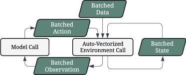
Figure 1: All operations during simulation occur on batched data. The environment step function is transformed with jax.vmap so it can operate on batches.

We use the JAX library to write the environment step function. The python JAX code can be just-in-time (jit) compiled and run efficiently in XLA on the GPU. However, for code to be jit-compilable some restrictions apply. First, all functions need to be pure, meaning they cannot have any side effects on global data. Practically, this is achieved by not saving any state in the environment, but instead passing in the current environment state and returning the updated state. Furthermore, the parallel processing on a GPU requires that exactly the same operations are conducted on all data points. Therefore, logical branches on the computation graph are allowed to be rewritten. The overall approach is to execute all code branches and select the required result after calculation. Even complex simulation features can be rewritten in this way. One example is our roads library, which provides useful information about the road, like lane boundary points. Example observations based on the roads library are depicted in Figure 7.

The automatic vectorization primitive jax.vmap simplifies writing parallelizable code. Functions can be written in lower dimensions and then vectorized without any modifications of the code. We use this primitive extensively across the simulation code. For example, we vectorize the entire environment step function this way. Applying the discussed principles leads to a jit-compilable update function that can run on a batch of data.

Finally, to maximize the simulation speed, we combine the batched environment call with the batched model call and scan along the time axis of the dynamic data via the jax.lax.scan primitive. The entire simulation is then jit-compiled into a single graph and run in XLA.

3.2.3 Achieving high scenario throughput

The implementation we have described so far is very fast for a single batch of scenarios. However, our goal is to run many different batches as fast as possible. To achieve this, we always pre-load the next batch from disk into GPU memory. When the simulation of the current batch is completed the next batch can immediately be simulated. Figure 2 shows this approach.

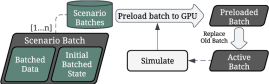
Figure 2: To achieve high GPU utilization one scenario batch is pre-loaded to the GPU memory while a simulation of a different batch is running.

3.2.4 Simulator performance benchmark

To demonstrate the performance of our simulator, we compare the environment step time with Waymax (Gulino et al., 2023), which is closest to our work. Table 1 reports the step time for different batch sizes on Nvidia v100 GPUs, showing that our simulator runs slightly faster.

Table 1: Runtime comparison for different batch sizes (BS) between Waymax (Gulino et al., 2023) and our simulator for one controlled agent.

		Step time [ms]
Simulator	Device	BS 1	BS 16
Waymax	v100	0.75	2.48
Ours	v100	0.52	0.82

3.3 RL problem formulation

For our reinforcement learning approach we need to specify how we retrieve the model inputs (observations) from the state $s$ and how we generate the physical actions from the model outputs. The state $s$ is the state of the simulation described previously, i.e., agents, roads, traffic lights etc. We also need to define the rewards, so the simulated data can be used to calculate the parameter update from an RL method. The rewards described below in section 3.3.3 are particularly challenging to specify, because the rewards define both the safety constraints of the learned policies while also encoding the goal of making progress along the desired route.

3.3.1 Observation space

The observation space retrieves a subset of the information of the environment state and transforms the fields of the observation vector into an agent-centric coordinate frame. We split up the observations into different modalities which can be found as model inputs in Figure 3. The observations of the active agent include the physical state, such as the current velocity and steering angle of the controlled agent, as well as stop line and traffic light information. For the closest agents, the pose of these agents relative to the active agent as well as the minimum bounding box distance are extracted. The number of agents increases from 64 to 256 depending on the model size. For the road network the closest 128 road elements, such as lane markings, stop lines, or crosswalks are selected. The route observations contain lane border points of up to 8 drivable lanes along the route. For each lane, up to 64 points are sampled between 20 m behind and 106 m ahead of the agent, allowing the agent to change lanes and to take the correct turns. The route and road network observations are depicted in Figure 7. For a better estimate of the state value, the remaining time in the episode is retrieved. It is only provided to the value head and not to the policy head of the model, because we observed that the policy learned to exploit this observation. For example, the policy learned to maneuver the agent into dangerous situations just before the end of the scenario, as it learned that it would be “rescued” by the episode ending.

3.3.2 Action space

Our model directly controls the longitudinal acceleration as well as the steering angle rate. Using these controls guarantees that the associated dynamic constraints are not violated. It also makes it easier to introduce comfort rewards on lateral and longitudinal acceleration. We are using discrete actions, which we found to be more stable than continuous actions during reinforcement learning training. The action space decodes each discrete action into the associated physical action. For example, the acceleration can take 71 different values between -4 $\nicefrac{{m}}{{s^{2}}}$ and 3 $\nicefrac{{m}}{{s^{2}}}$. During training an action is sampled according to the probability distribution. For evaluation the greedy action is selected.

3.3.3 Rewards

The goal of the policy is to navigate safely through traffic. In particular, the agent should make progress along the desired route while not colliding with other agents and adhering to basic traffic rules. In order to achieve this, we introduce dense rewards as well as done signals that are associated with sparse rewards.

The done signals terminate an episode immediately and are introduced for safety critical failures to avoid any trade off between safety and progress. For example, running a red light could be beneficial if it allows the agent to gain a lot of reward for making progress afterwards. Done signals have been introduced for collisions, off-route driving, as well as running red lights and stop lines and are associated with high negative rewards. The done signals are only enabled for training but not for evaluation. This is required to compare our results to the current SOTA (Lu et al., 2023) which does not terminate the episode in the described events.

Dense rewards are introduced for the progress along the planned route (positive), velocity above the speed limit, as well as on the squared lateral and longitudinal acceleration (all negative).

3.4 Distributed learning system

With the generated scenarios, the efficient simulator, and reward model, we can establish the reinforcement learning approach. Our base reinforcement learner uses actor-critic Proximal Policy Optimization (PPO) (Schulman et al., 2017). However, just as we distribute our simulator to achieve scale, we also require a distributed training framework which runs training and simulation asynchronously. This in turn introduces challenges for actor-critic methods which are by nature on-policy methods. Furthermore, we want to pre-train a policy via behavioral cloning, similar to AlphaStar (Vinyals et al., 2019) since a good initial policy can speed up the RL training. However, only pre-training the policy and not the value network poses challenges to the stability at the start of RL training which we need to overcome. We describe the overall model architecture in section 3.4.1, followed by how we perform pre-training in section 3.4.2 and finally the distributed actor-critic learner in section 3.4.3.

3.4.1 Model architecture

The inputs from section 3.3.1 are given to an attention-based (Vaswani et al., 2023) observation encoder which successively cross attends all the modalities (Jaegle et al., 2021; Bronstein et al., 2022a). The output of this encoder is then fed into the policy head, which is a stack of dense residual blocks for both actions followed by an output layer of required size for the given action. For the value head, the encoder output is first concatenated with the embedded value function observations. The concatenated array is then passed into dense residual blocks and a final layer of size one in order to obtain the scalar state value estimation. The model architecture is depicted in Figure 3.

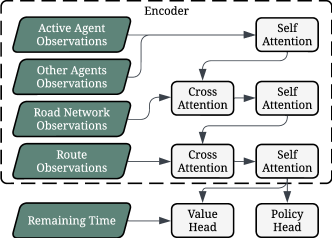
Figure 3: Perceiver-style model architecture. Starting with self attention across all agents, followed by cross attention of all other modalities. The encoder weights are shared between the policy and value network.

3.4.2 Pre-training via supervised learning

Pre-training only the policy via behavioral cloning makes it challenging to further train this policy with an actor-critic RL method (Uchendu et al., 2023). The untrained critic network can lead to policy updates that destroy the policy. Therefore, we decided to pre-train the policy as well as the value network. We leverage our simulator by replaying the original trajectories and retrieving the rewards $R(s_{t})$ as defined for the RL problem (where $s$ is the state space, i.e., the state of the simulation as described previously). With the rewards we can estimate the value function target by the discounted return $G$ as

$$V_{target}(s_{0})=G_{0}=\sum_{t=0}^{T}\gamma^{t}R(s_{t}).$$ (1)

The total supervised loss is the combination of the cross-entropy loss for the discrete actions and the mean squared error between the predicted state value and the previously estimated value function target. To achieve high throughput, particularly with increasing model size, the pre-training is scaled to many machines using NVIDIA NCCL.

3.4.3 Fine tuning via reinforcement learning

We set up an asynchronous reinforcement learning system similar to Dota2 (Berner et al., 2019). The asynchronous setting allows to run the learners and actors independently avoiding any slow down. Therefore, the training speed scales linearly with the number of machines as shown in Appendix C. This allows us to run experiments with billions of agent steps even with increasing model size. Multiple actors gather experience in parallel using the latest available policy at the beginning of each episode. Multiple learners are created using many GPUs across multiple machines. Each learner creates its own replay table which receives experience from a subset of actors that are assigned to this learner. This avoids any gRPC bottlenecks of a single replay table design. Communication across the groups of learners, replay tables, and associated actors only occurs when calculating the mean gradient update via NVIDIA NCCL. An additional evaluation actor periodically runs a smaller evaluation dataset to obtain metrics of the current policy throughout the training process. The described system design is shown in Figure 4.

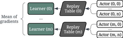
Figure 4: The distributed reinforcement learning framework consists of many groups of learners, replay tables, and actors. The gradients are synchronized across the different learners via NVIDIA NCCL.

The policy is trained using Proximal Policy Optimization (PPO) (Schulman et al., 2017). However, because of the asynchronous training setup as well as updating the actor-parameters only before each episode learning becomes off-policy. To address this challenge, we use the V-trace off-policy correction algorithm (Espeholt et al., 2018).

4 Evaluation

This section describes the different metrics and the dataset used for policy evaluation and comparison.

4.1 Metrics

The goal of the metrics are to measure the quality of the trained policy. This is already a complex problem for autonomous driving as the quality of driving comprises many different aspects. For the scope of this paper, we follow the work of Lu et al. (2023) who introduced the failure rate and progress ratio as relevant metrics for autonomous driving. The failure rate measures the fundamental safety of the policy. If the agent collides or drives off-road in the simulation the scenario is considered as failed. The failure rate is the percentage of failed scenarios across the entire evaluation dataset. Our implementation uses an off-route signal which has stricter constraints than the off-road criterion used by Lu et al. (2023), which might slightly overestimate our failure rates. The progress ratio is the distance traveled by the agent in the simulation divided by the distance traveled of the vehicle in the original log. When the agent travels the same distance as the vehicle in the log, this metric becomes 100 %. Higher values indicate that the agent makes more progress than the reference vehicle. Overall a higher value is better, however only when the policy is also safe.

In addition to collisions and off-route failures, we also implemented metrics for stop line and traffic light violations. We did not include these violations in the failure rate to maintain consistency with previously reported results. However, we do report these metrics in Table 2.

4.2 Dataset

As the current state-of-the-art policies (Lu et al., 2023) are evaluated on proprietary datasets, our goal was to achieve the fairest comparison by following the same dataset mining procedure. A dataset of 10k randomly sampled 10 s segments was created using data collected from human-expert driving in San Francisco. This is comparable to the ”All” evaluation dataset in Lu et al. (2023).

5 Experiments

Combining the real-world driving simulator, the scalable reinforcement learning framework and the described evaluation metrics and dataset, we conduct experiments with different training dataset and model sizes. For all these experiments we keep the hyperparameters the same. In particular we run our experiments for larger models across more GPUs to achieve the same batch size. The hyperparameters for all experiments can be found in Appendix E.

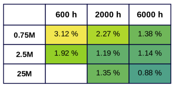
(a) Minimum failure rate

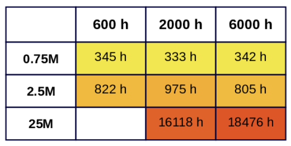
(b) GPU time

Figure 5: Results for experiments with different model sizes (rows) and dataset sizes (columns). Colors represent the numerical results on color scales. (a) The performance of the policy improves with increasing model and dataset size. (b) The model size is the major driver of the required GPU time and therefore cost of training. Dataset size has no effect on the training time, but it can affect one time costs during data preprocessing which is not considered here.

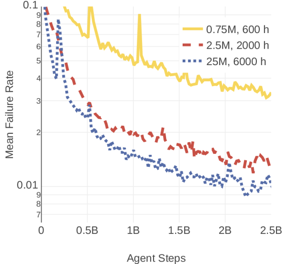
(a) Failure Rate

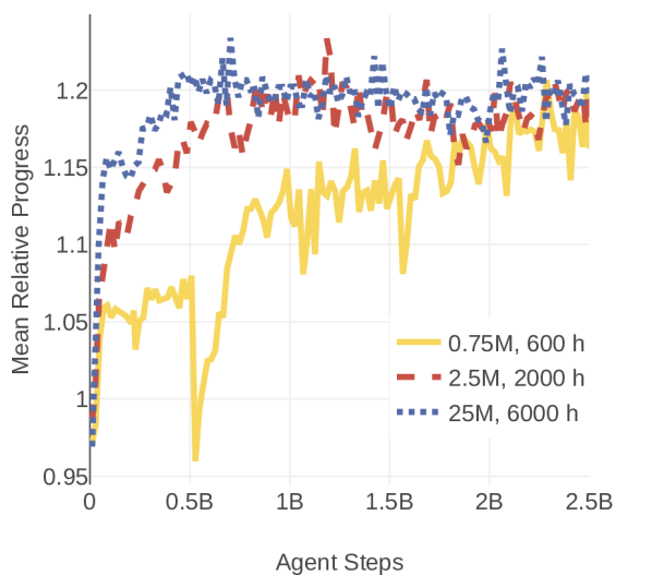
(b) Progress Ratio

Figure 6: Training curves showing the failure rate and progress ratio when scaling model and dataset size.

We mined three different training datasets of 600 h, 2000 h and 6000 h from human-expert driving in San Francisco. We also created three different model sizes of 0.75M, 2.5M and 25M parameters by increasing the attention dimensions of the network described in section 3.4.1. Each model is trained first by behavior cloning for 20 epochs on the given dataset. The pre-trained policy is then refined by reinforcement learning on 2.5B agent steps. We evaluate the policy during reinforcement learning every 20M agent steps and after training select the checkpoint with the lowest failure rate on the evaluation dataset.

We conduct experiments on all combinations of model size and dataset size, with the exception of the small 600 h dataset in combination with the large 25M parameter model. 5(a) shows that increasing the dataset size improves the performance of the trained policy in terms of failure rate. Increasing the model size in general also improves the policy performance. The 2.5M model is strictly better than the 0.75M model and the best policy is trained on the 25M model. However, we observe that increasing the model size only helps when sufficient real-world driving data is available. On the 2000 h dataset the 25M performs worse than the 2.5M model and only on the 6000 h dataset it performs better. The largest experiment achieves a failure rate of 0.88 %, and outperforms SOTA and other baselines as shown in Table 2.

The dataset and model size have a very different effect on the total GPU time as shown in 5(b). The model size is the main driver for increased GPU time. It requires more GPUs to train and run inference on the same batch size and also slows down each training step and inference call. For example training the large 25M model is about 20 times as expensive as training the medium 2.5M model. In contrast to that, the dataset size has no effect on the reinforcement learning GPU time.

Table 2: Comparison of our policies with the current SOTA (Lu et al., 2023).

	BC (Lu et al., 2023)	MGAIL (Lu et al., 2023)	SAC (Lu et al., 2023)	BC+SAC (Lu et al., 2023)	Our BC	Our BC+PPO
Failure Rate [%] (Lu et al., 2023)	3.64	2.45	5.60	2.81	19.85	0.88
Progress Ratio [%] (Lu et al., 2023)	98.1	96.6	71.1	87.6	96.91	120.8
Collisions [%]	-	-	-	-	10.32	0.46
Off-Route Events [%]	-	-	-	-	10.35	0.49
Stop Line Violations [%]	-	-	-	-	2.47	0.02
Traffic Light Violations [%]	-	-	-	-	2.08	0.28

It is important to note that increasing the dataset size does not come entirely for free. Compute cost for data preprocessing, the required disk storage size as well as network usage increase. However, preprocessing can be considered a one time cost, because the data can be reused for variations of the experiment. Disk space and network usage did not become a bottleneck in our setting.

We provide training curves for simultaneously scaling the dataset and model size in Figure 6. The curves on the left (6(a)) show that the failure rate in all settings continuously improves over the course of training. The larger experiments converge to lower failure rates and the lowest failure rate of 0.88 % for the 25M model in combination with the 6000 h dataset is achieved after 2.2B agent steps. The progress ratio for the same experiments is depicted in 6(b). All experiments achieve a progress ratio of about 120 % towards the end of training. This shows that our trained policies are achieving low failure rates while also making more progress than the human-driven reference.

In Table 2 we compare the policy performance of our largest setting after behavioral cloning and after reinforcement learning training with the current SOTA (Lu et al., 2023). Our behavioral cloning policy performs quite poorly, achieving a failure rate of 19.85 %. This is much higher than the pure BC failure rate of 3.64 % reported in the current SOTA (Lu et al., 2023).

As previously discussed, the reinforcement learning training improves the policy and achieves a failure rate of 0.88 % and a progress ratio of 120.8 %. Compared to the best policy of the current SOTA on a similar dataset, the failure rate is reduced by 64% and the progress ratio improved by 25%.

Table 2 also lists the rate of collisions, off-route events, stop line violations, and traffic light violations separately. As mentioned in section 4.1, stop line violations (0.02 %) and traffic light violations (0.28 %) are not counted towards the failure rate for comparison reasons to the current SOTA (Lu et al., 2023). Because the done signals are disabled for evaluation, a single scenario can contain a collision and an off-route event. Therefore, the sum of the collision rate (0.46 %) and the off-route event rate (0.49 %) is slightly higher than the failure rate (0.88 %).

6 Conclusions

In this paper we combined an efficient and realistic autonomous driving simulator with a scalable reinforcement learning framework. This allowed us to run large scale reinforcement learning experiments training on billions of agents steps with increasing model size on different dataset sizes of real-world driving.

Our data shows that we can obtain similar scaling behavior as in other reinforcement learning settings (Hilton et al., 2023) when using increasingly large datasets of real-world driving. In particular, we were able to obtain better policies with larger models when using sufficiently large datasets. Our best policy reduces the failure rate compared to the current SOTA (Lu et al., 2023) by 64% while improving progress by 25%. These results are very encouraging, and motivate further experiments with increasing size. However, to ultimately answer whether the presented approach can be scaled beyond human performance a validation framework that can reliably compare the safety of the policy to human drivers is also required.

While the goal of this work was to train a policy that maximizes safety, retaining natural driving behavior is also required for safe interaction with human drivers. Therefore, methods constraining the divergence of the RL policy from the IL policy, such as concurrent training (Lu et al., 2023) or additional loss terms based on the divergence (Vinyals et al., 2019) should be investigated.

Another area for future work is the scenario divergence. Conducted experiments with heuristics to combat unrealistic agent behavior showed that the policy is able to exploit these heuristics, leading ultimately to worse results. We showed that we can overcome the issue of non-reactive agents by training on a large dataset. Reducing scenario divergence will probably improve metrics accuracy, therefore better guiding future research efforts. The improved data quality from reactive agents might also be beneficial for training. However, further research is required on how to overcome the exploitation of agent reactiveness.

With our approach we were able to achieve failure rates below one percent. This leads to only about 60 hours of our largest 6000 h dataset being relevant to further improve the safety of the policy. Creating a much larger dataset, quantifying the scenario difficulty of the contained scenarios, and over sampling difficult scenarios might improve failure rate even more.

7 Impact Statement

This paper presents work whose goal is to advance the field of Machine Learning by demonstrating how scalable simulation and reinforcement learning may be achieved to learn control policies for autonomous embodied agents acting in the real world. We are committed to democratizing transportation broadly, and how transportation affects people’s lives. We believe that autonomous embodied agents are an important technology on the path to realizing that vision and the work in this paper is a step along that path.

Appendix A Roads observations

The implemented roads library in our simulator delivers important information for our rewards and observations. For example, it can calculate the distance to the next stop line. We also use it to create observations of the route and the nearby road segments. This is illustrated in Figure 7.

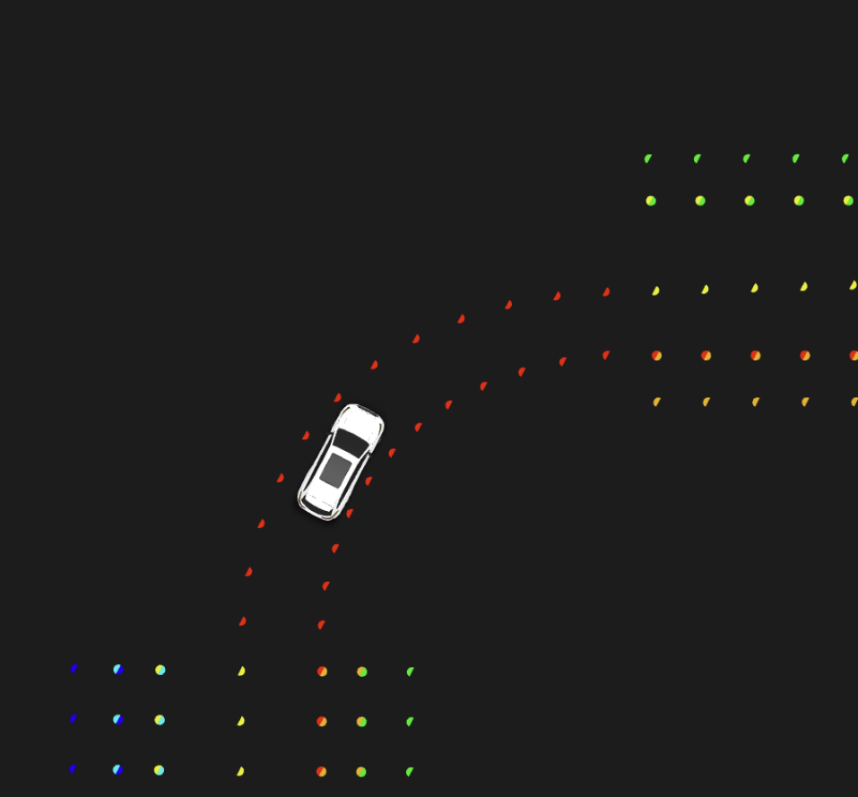
(a) Route border points of all drivable lanes. Only one lane is a valid connection for the right turn the agent is performing. Before and after the turn, other lanes are also valid.

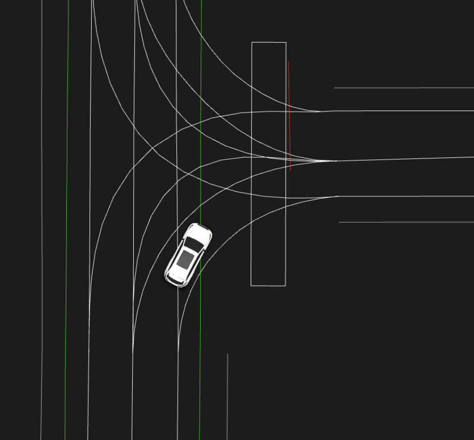
(b) Road network points visualized by poly-lines. The color depends on the properties of the annotation, for example the stop line being visualized in red and bike lane boundaries in green.

Figure 7: Route and road network observations obtained from the roads library.

Appendix B Metric validation

We validated the collision and off-route detection by taking 25 positive and 25 negative samples for each metric from the validation dataset. These have been inspected by human triagers to confirm whether the metric is correct. For the collision and the off-route detection this validation found that all 50 scenarios for each metric were labeled correctly according to our definition. However, overall both metrics were found to be conservative, leading potentially to higher failure rates.

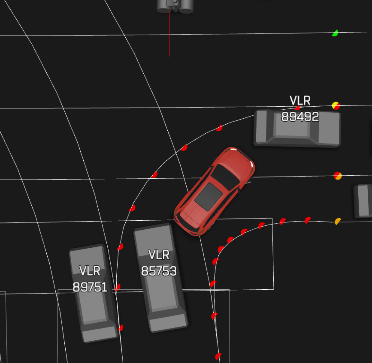
(a) Detected collision with agent 85753 because of the conservative bounding box check.

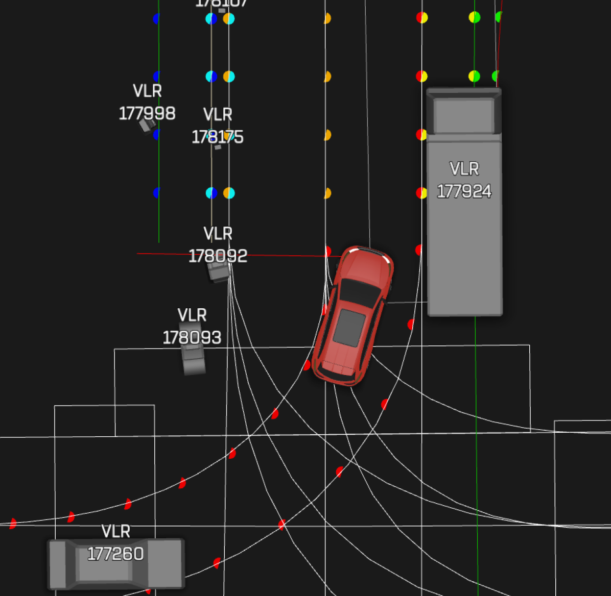
(b) Overly restrictive lane permissibility in a junction. Off-route event detected due to increased bounding box size.

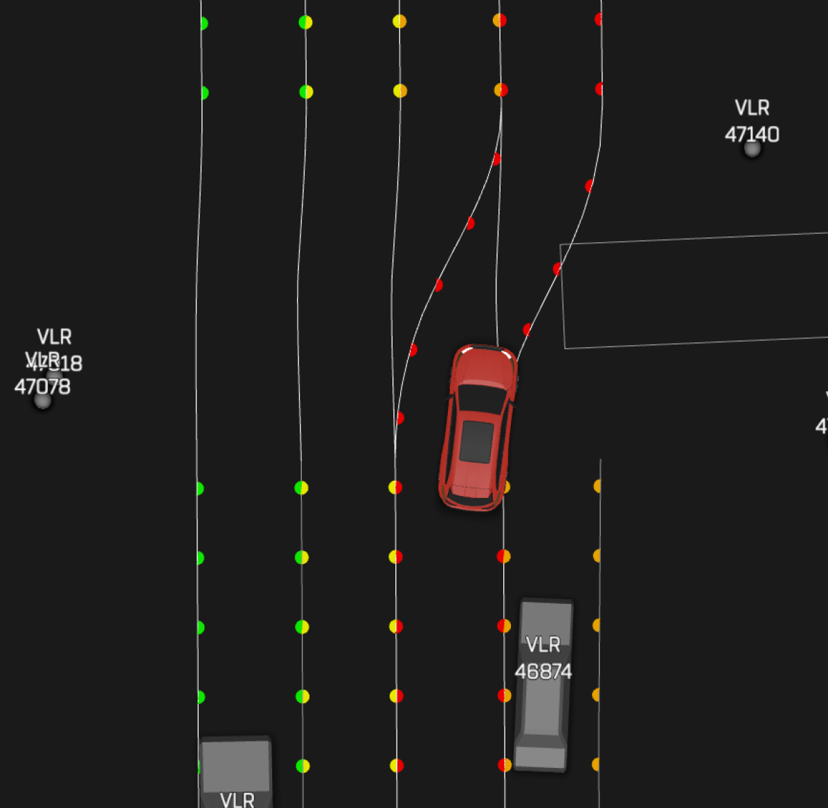
(c) Overly restrictive lane permissibility on a road segment with branching lanes.

Figure 8: Examples of conservative detection of collisions and off-route events.

For the collision-free metric a bounding box approximating the vehicle is checked against the bounding box of other vehicles. As the bounding box includes all parts of the vehicle, for example the mirrors and sensors, checking collisions against the bounding box is conservative. 8(a) illustrates this conservative check.

In many situations the permissible lane along the route is overly restrictive leading to off-route events. This occurs particularly in junctions (8(b)) and lane merges or branches (8(c)). Human expert drivers were found to not exactly follow these lane geometries either. Future work to relax the conditions in these cases to the entire drivable surface is required. On top of that, the check is also on the conservative side due to the increased bounding box size.

Appendix C Framework scalability

When scaling experiments to more GPUs it is important that the policy performance is not affected and that the overall runtime is reduced. Ideally, the reduction in runtime is inversely proportional to the number of GPUs used, so the overall GPU time and, therefore, the cost to run the experiment stays the same. Table 3 shows the results for experiments running on 8, 16, and 32 machines. The overall policy performance is very similar and the differences can be considered noise. The overall GPU time sees a marginal uptick. We calculated the normalized GPU time by dividing the total GPU time by the total GPU time of the 8-GPU experiment. As the numbers are close to 1, the framework scales almost perfectly.

Table 3: Runtime and policy performance metrics for experiments running on different numbers of GPUs. The policy performance is very similar, but the runtime goes down as expected.

Number of GPUs	8	16	32
Runtime [h]	$41.58$	$21.94$	$11.99$
Total GPU time [h]	$332.6$	$351.0$	$383.7$
Normalized GPU time	$1$	$1.05$	$1.15$
Failure Rate	$1.28$	$1.25$	$1.45$

Appendix D Ablation of SL pre-training

For this ablation we removed the SL pre-training in order to understand the effectiveness of this step. We used the large 6000 h dataset, the 2.5M model and again trained on 2.5B agent steps.

Even without the SL pre-training the agent can learn to make progress and reduce the failure rate over the course of training as depicted in Figure 9. However, after 2.5B agent steps the policy without pre-training is still at about 2 % failure rate, which the pre-trained policy reached already after 0.5B steps. Also the failure rate at 2.5B agent steps is lower for the policy that has been pre-trained. The increased training speed is also observed for the progress ratio. The pre-trained policy reaches values around 120 % after 0.5B steps and the policy without pre-training catches up to that value at around 2.5B steps. These results overall confirm the effectiveness of the pre-training step in terms of speed. Pre-training also helps to reach better final performance in terms of safety.

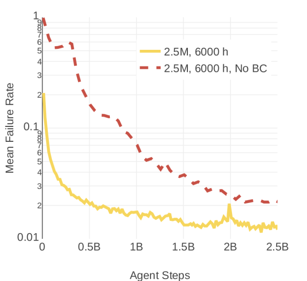
(a) Failure Rate

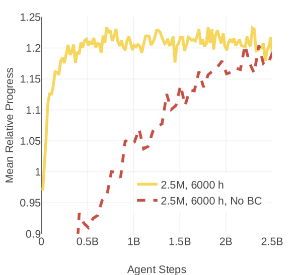
(b) Progress Ratio

Figure 9: Training curves for experiments with and without the SL pre-training on the 2.5M parameter model and the 6000 h dataset.

Appendix E Hyperparameters

Table 4 shows the most important hyperparameters for both the behavioral cloning stage and the reinforcement learning stage.

Table 4: BC and RL Hyperparameters

	BC	RL
Batch size	$32768$	$512$
Sequence length	-	32
Learning rate	$2*10^{-3}$	$5.6*10^{-5}$
PPO clip param	-	$0.3$
Value loss scaling	$10^{-4}$	$10^{-2}$
PPO entropy coefficient	-	$3*10^{-2}$

References

- Berner et al. (2019) Berner, C., Brockman, G., Chan, B., Cheung, V., Debiak, P., Dennison, C., Farhi, D., Fischer, Q., Hashme, S., Hesse, C., Józefowicz, R., Gray, S., Olsson, C., Pachocki, J., Petrov, M., d. O. Pinto, H. P., Raiman, J., Salimans, T., Schlatter, J., Schneider, J., Sidor, S., Sutskever, I., Tang, J., Wolski, F., and Zhang, S. Dota 2 with large scale deep reinforcement learning, 2019.
- Bronstein et al. (2022a) Bronstein, E., Palatucci, M., Notz, D., White, B., Kuefler, A., Lu, Y., Paul, S., Nikdel, P., Mougin, P., Chen, H., Fu, J., Abrams, A., Shah, P., Racah, E., Frenkel, B., Whiteson, S., and Anguelov, D. Hierarchical model-based imitation learning for planning in autonomous driving, 2022a.
- Bronstein et al. (2022b) Bronstein, E., Srinivasan, S., Paul, S., Sinha, A., O’Kelly, M., Nikdel, P., and Whiteson, S. Embedding synthetic off-policy experience for autonomous driving via zero-shot curricula, 2022b.
- Dosovitskiy et al. (2017) Dosovitskiy, A., Ros, G., Codevilla, F., Lopez, A., and Koltun, V. Carla: An open urban driving simulator, 2017.
- Espeholt et al. (2018) Espeholt, L., Soyer, H., Munos, R., Simonyan, K., Mnih, V., Ward, T., Doron, Y., Firoiu, V., Harley, T., Dunning, I., Legg, S., and Kavukcuoglu, K. Impala: Scalable distributed deep-rl with importance weighted actor-learner architectures, 2018.
- Gulino et al. (2023) Gulino, C., Fu, J., Luo, W., Tucker, G., Bronstein, E., Lu, Y., Harb, J., Pan, X., Wang, Y., Chen, X., Co-Reyes, J. D., Agarwal, R., Roelofs, R., Lu, Y., Montali, N., Mougin, P., Yang, Z., White, B., Faust, A., McAllister, R., Anguelov, D., and Sapp, B. Waymax: An accelerated, data-driven simulator for large-scale autonomous driving research, 2023.
- Hilton et al. (2023) Hilton, J., Tang, J., and Schulman, J. Scaling laws for single-agent reinforcement learning, 2023.
- Igl et al. (2022) Igl, M., Kim, D., Kuefler, A., Mougin, P., Shah, P., Shiarlis, K., Anguelov, D., Palatucci, M., White, B., and Whiteson, S. Symphony: Learning realistic and diverse agents for autonomous driving simulation, 2022.
- Jaegle et al. (2021) Jaegle, A., Gimeno, F., Brock, A., Zisserman, A., Vinyals, O., and Carreira, J. Perceiver: General perception with iterative attention, 2021.
- Li et al. (2022) Li, Q., Peng, Z., Feng, L., Zhang, Q., Xue, Z., and Zhou, B. Metadrive: Composing diverse driving scenarios for generalizable reinforcement learning, 2022.
- Lu et al. (2023) Lu, Y., Fu, J., Tucker, G., Pan, X., Bronstein, E., Roelofs, R., Sapp, B., White, B., Faust, A., Whiteson, S., Anguelov, D., and Levine, S. Imitation is not enough: Robustifying imitation with reinforcement learning for challenging driving scenarios, 2023.
- Schulman et al. (2017) Schulman, J., Wolski, F., Dhariwal, P., Radford, A., and Klimov, O. Proximal policy optimization algorithms, 2017.
- Uchendu et al. (2023) Uchendu, I., Xiao, T., Lu, Y., Zhu, B., Yan, M., Simon, J., Bennice, M., Fu, C., Ma, C., Jiao, J., Levine, S., and Hausman, K. Jump-start reinforcement learning, 2023.
- Vaswani et al. (2023) Vaswani, A., Shazeer, N., Parmar, N., Uszkoreit, J., Jones, L., Gomez, A. N., Kaiser, L., and Polosukhin, I. Attention is all you need, 2023.
- Vinitsky et al. (2023) Vinitsky, E., Lichtlé, N., Yang, X., Amos, B., and Foerster, J. Nocturne: a scalable driving benchmark for bringing multi-agent learning one step closer to the real world, 2023.
- Vinyals et al. (2019) Vinyals, O., Babuschkin, I., Czarnecki, W. M., Mathieu, M., Dudzik, A., Chung, J., Choi, D. H., Powell, R., Ewalds, T., Georgiev, P., Oh, J., Horgan, D., Kroiss, M., Danihelka, I., Huang, A., Sifre, L., Cai, T., Agapiou, J. P., Jaderberg, M., Vezhnevets, A. S., Leblond, R., Pohlen, T., Dalibard, V., Budden, D., Sulsky, Y., Molloy, J., Paine, T. L., Gulcehre, C., Wang, Z., Pfaff, T., Wu, Y., Ring, R., Yogatama, D., Wünsch, D., McKinney, K., Smith, O., Schaul, T., Lillicrap, T., Kavukcuoglu, K., Hassabis, D., Apps, C., and Silver, D. Grandmaster level in starcraft ii using multi-agent reinforcement learning. Nature, 575(7782):350–354, 2019.
- Vitelli et al. (2021) Vitelli, M., Chang, Y., Ye, Y., Wołczyk, M., Osiński, B., Niendorf, M., Grimmett, H., Huang, Q., Jain, A., and Ondruska, P. Safetynet: Safe planning for real-world self-driving vehicles using machine-learned policies, 2021.
- Zhang et al. (2023) Zhang, C., Tu, J., Zhang, L., Wong, K., Suo, S., and Urtasun, R. Learning realistic traffic agents in closed-loop, 2023.
- Zhang et al. (2021) Zhang, Z., Liniger, A., Dai, D., Yu, F., and Gool, L. V. End-to-end urban driving by imitating a reinforcement learning coach, 2021.