On elementary cellular automata asymptotic (a)synchronism sensitivity and complexity

Abstract

Among the fundamental questions in computer science is that of the impact of synchronism/asynchronism on computations, which has been addressed in various fields of the discipline: in programming, in networking, in concurrence theory, in artificial learning, etc. In this paper, we tackle this question from a standpoint which mixes discrete dynamical system theory and computational complexity, by highlighting that the chosen way of making local computations can have a drastic influence on the performed global computation itself. To do so, we study how distinct update schedules may fundamentally change the asymptotic behaviors of finite dynamical systems, by analyzing in particular their limit cycle maximal period. For the message itself to be general and impacting enough, we choose to focus on a “simple” computational model which prevents underlying systems from having too many intrinsic degrees of freedom, namely elementary cellular automata. More precisely, for elementary cellular automata rules which are neither too simple nor too complex (the problem should be meaningless for both), we show that update schedule changes can lead to significant computational complexity jumps (from constant to superpolynomial ones) in terms of their temporal asymptotes.

1 Introduction

In the domain of discrete dynamical systems at the interface with computer science, the generic model of automata networks, initially introduced in the 1940s through the seminal works of McCulloch and Pitts on formal neural networks [20] and of Ulam and von Neumann on cellular automata [30], has paved the way for numerous fundamental developments and results; for instance with the introduction of finite automata [17], the retroaction cycle theorem [26], the undecidability of all nontrivial properties of limit sets of cellular automata [15], the Turing universality of the model itself [28, 11], … and also with the generalized use of Boolean networks as a representational model of biological regulation networks since the works of Kauffman [16] and Thomas [29]. Informally speaking, automata networks are collections of discrete-state entities (the automata) interacting locally with each other over discrete time which are simple to define at the static level but whose global dynamical behaviors offer very interesting intricacies.

Despite major theoretical contributions having provided since the 1980s a better comprehension of these objects [27, 11] from computational and behavioral standpoints, understanding their sensitivity to (a)synchronism remains an open question on which any advance could have deep implications in computer science (around the thematics of synchronous versus asynchronous computation and processing [2, 3]) and in systems biology (around the temporal organization of genetic expression [13, 10]). In this context, numerous studies have been published by considering distinct settings of the concept of synchronism/asynchronism, i.e. by defining update modes which govern the way automata update their state over time. For instance, (a)synchronism sensitivity has been studied per se according to deterministic and non-deterministic semantics in [12, 1, 21] for Boolean automata networks and in [14, 9, 7, 8] for cellular automata subject to stochastic semantics.

In these lines, the aim of this paper is to increase the knowledge on Boolean automata networks and cellular automata (a)synchronism sensitivity. To do so, we choose to focus on the impact of different kinds of periodic update modes on the dynamics of elementary cellular automata: from the most classical parallel one to the more general local clocks one [22]. Because we want to exhibit the very power of update modes on dynamical systems and concentrate on it, the choice of elementary cellular automata is quite natural: they constitute a restricted and “simple” cellular automata family which is well known to have more or less complex representatives in terms of dynamical behaviors  [31, 4, 18] without being too much permissive. For our study, we use an approach derived from [25] and we pay attention to the influence of update modes on the asymptotic dynamical behaviors they can lead to compute, in particular in terms of limit cycles maximal periods.

In this paper, we highlight formally that the choice of the update mode can have a deep influence on the dynamics of systems. In particular, two specific elementary cellular automata rules, namely rules $156$ and $178$ (a variation of the well-known majority function tie case) as defined by the Wolfram’s codification, are studied here. They have been chosen from the experimental classification presented in [31], as a result of numerical simulations which have given the insight that they are perfect representatives for highlighting (a)synchronism sensitivity. Notably, they all belong to the Wolfram’s class II, which means that, according to computational observations, these cellular automata evolved asymptotically towards a “set of separated simple stable or periodic structures”. Since our (a)synchronism sensitivity measure consists in limit cycles maximal periods, this Wolfram’s class II is naturally the most pertinent one in our context. Indeed, class I cellular automata converge to homogeneous fixed points, class III cellular automata leads to aperiodic or chaotic patterns, and class IV cellular automata, which are deeply interesting from the computational standpoint, are not relevant for our concern because of their global high expressiveness which would prevent from showing asymptotic complexity jumps depending on update modes. On this basis, for these two rules, we show between which kinds of update modes asymptotic complexity changes appear. What stands out is that each of these rules admits it own (a)synchronism sensitivity scheme (which one could call its own asymptotic complexity scheme with respect to synchronism), which supports interestingly the existence of a periodic update modes expressiveness hierarchy.

In Section 2, the main definitions and notations are formalized. The emphasizing of elementary cellular automata (a)synchronism sensitivity is presented in Section 3 through upper-bounds for the limit-cycle periods of rules $156$ and $178$ depending on distinct families of periodic update modes. The paper ends with Section 4 in which we discuss some perspectives of this work. Full proofs can be found in the long version of this paper available here.

2 Definitions and notations

General notations

Let $\llbracket n\rrbracket=\{0,\ldots,n-1\}$, let $\mathbb{B}=\{0,1\}$, and let $x_{i}$ denote the $i$-th component of vector $x\in\mathbb{B}^{n}$. Given a vector $x\in\mathbb{B}^{n}$, we can denote it classically as $(x_{0},\dots,x_{n-1})$ or as the word $x_{0}\dots x_{n-1}$ if it eases the reading.

2.1 Boolean automata networks and elementary cellular automata

Roughly speaking, a Boolean automata network (BAN) applied over a grid of size $n$ is a collection of $n$ automata represented by the set $\llbracket n\rrbracket$, each having a state within $\mathbb{B}$, which interact with each other over discrete time. A configuration $x$ is an element of $\mathbb{B}^{n}$, i.e.a Boolean vector of dimension $n$. Formally, a BAN is a function $f:\mathbb{B}^{n}\to\mathbb{B}^{n}$ defined by means of $n$ local functions $f_{i}:\mathbb{B}^{n}\to\mathbb{B}$, with $i\in\llbracket n\rrbracket$, such that $f_{i}$ is the $i$th component of $f$. Given an automaton $i\in\llbracket n\rrbracket$ and a configuration $x\in\mathbb{B}^{n}$, $f_{i}(x)$ defines the way that $i$ updates its states depending on the state of automata effectively acting on it; automaton $j$ “effectively” acts on $i$ if and only if there exists a configuration $x$ in which the state of $i$ changes with respect to the change of the state of $j$; $j$ is then called a neighbor of $i$.

An elementary cellular automaton (ECA) is a particular BAN dived into the cellular space $\mathbb{Z}$ so that (i) the evolution of state $x_{i}$ of automaton $i$ (rather called cell $i$ in this context) over time only depends on that of cells $i-1$, $i$ itself, and $i+1$, and (ii) all cells share the same and unique local function. As a consequence, it is easy to derive that there exist $\smash{2^{2^{3}}}=256$ distinct ECA, and it is well known that these ECA can be grouped into $88$ equivalence classes up to symmetry.

In absolute terms, BANs as well as ECA can be studied as infinite models of computation, as it is classically done in particular with ECA. In this paper, we choose to focus on finite ECA, which are ECA whose underlying structure can be viewed as a torus of dimension $1$ which leads naturally to work on $\mathbb{Z}/n\mathbb{Z}$, the ring of integers modulo $n$ so that the neighborhood of cell $0$ is $\{n-1,0,1\}$ and that of cell $n-1$ is $\{n-2,n-1,0\}$.

Now the mathematical objects at stake in this paper are statically defined, let us specify how they evolve over time, which requires defining when the cells state update, by executing the local functions.

 

Figure 1: Illustration of the execution over time of local transition functions of any BAN $f$ of size $4$ according to (top left) $\mu_{\textsc{bs}}=(\{0\},\{2,3\},\{1\})$, (top right center) $\mu_{\textsc{bp}}=\{(1),(2,0,3)\}$, and (bottom) $\mu_{\textsc{lc}}=((1,3,2,2),(0,2,1,0))$. The $\checkmark$ symbols indicate the moments at which the automata update their states; the vertical dashed lines separate periodical time steps from each other.

2.2 Update modes

To choose an organization of when cells update their state over time leads to define what is classically called an update mode (aka update schedule or scheme). In order to increase our knowledge on (a)synchronism sensitivity, as evoked in the introduction, we pay attention in this article to deterministic and periodic update modes. Generally speaking, given a BAN $f$ applied over a grid of size $n$, a deterministic (resp. periodic) update mode of $f$ is an infinite (resp. a finite) sequence $\mu=(B_{k})_{k\in\mathbb{N}}$ (resp. $\mu=(B_{0},\dots,B_{p-1})$), where $B_{i}$ is a subset of $\llbracket n\rrbracket$ for all $i\in\mathbb{N}$ (resp. for all $i\in\llbracket p\rrbracket$). Another way of seeing the update mode $\mu$ is to consider it as a function $\mu^{\star}:\mathbb{N}\to\powerset(\llbracket n\rrbracket)$ which associates each time step with a subset of $\llbracket n\rrbracket$ so that $\mu^{\star}(t)$ gives the automata which update their state at step $t$; furthermore, when $\mu$ is periodic, there exists $p\in\mathbb{N}$ such that for all $t\in\mathbb{N}$, $\mu^{\star}(t+p)=\mu^{\star}(t)$.

Three known update mode families are considered: the block-sequential [27], the block-parallel [6, 23] and the local clocks [24] ones. Updates induced by each of them over time are depicted in Figure 1.

A block-sequential update mode $\mu_{\textsc{bs}}=(B_{0},\dots,B_{p-1})$ is an ordered partition of $\llbracket n\rrbracket$, with $B_{i}$ a subset of $\llbracket n\rrbracket$ for all $i$ in $\llbracket p\rrbracket$. Informally, $\mu_{\textsc{bs}}$ defines an update mode of period $p$ separating $\llbracket n\rrbracket$ into $p$ disjoint blocks so that all automata of a same block update their state in parallel while the blocks are iterated in series. The other way of considering $\mu_{\textsc{bs}}$ is: $\forall t\in\mathbb{N},\mu_{\textsc{bs}}^{\star}(t)=B_{t\mod p}$.

A block-parallel update mode $\mu_{\textsc{bp}}=\{S_{0},\dots,S_{s-1}\}$ is a partitioned order of $\llbracket n\rrbracket$, with $S_{j}=(i_{j,k})_{0\leq k\leq|S_{j}|-1}$ a sequence of $\llbracket n\rrbracket$ for all $j$ in $\llbracket s\rrbracket$. Informally, $\mu_{\textsc{bp}}$ separates $\llbracket n\rrbracket$ into $s$ disjoint subsequences so that all automata of a same subsequence update their state in series while the subsequences are iterated in parallel. Note that there exists a natural way to convert $\mu_{\textsc{bp}}$ into a sequence of blocks of period $p=\text{lcm}(|S_{0}|,\dots,|S_{s-1}|)$. It suffices to define function $\varphi$ as: $\varphi(\mu_{\textsc{bp}})=(B_{\ell})_{\ell\in\llbracket p\rrbracket}$ with $B_{\ell}=\{i_{j,\ell\mod|S_{j}|}\mid j\in\llbracket s\rrbracket\}$. The other way of considering $\mu_{\textsc{bp}}$ is: $\forall j\in\llbracket s\rrbracket,\forall k\in\llbracket|S_{j}|\rrbracket$, $i_{j,k}\in\mu_{\textsc{bp}}^{\star}(t)\iff k=t\mod|S_{j}|$.

A local clocks update mode $\mu_{\textsc{lc}}=(P,\Delta)$, with $P=(p_{0},\dots,p_{n-1})$ and $\Delta=(\delta_{0},\dots,\delta_{n-1})$, is an update mode such that each automaton $i$ of $\llbracket n\rrbracket$ is associated with a period $p_{i}\in\mathbb{N}^{*}$ and an initial shift $\delta_{i}\in\llbracket p_{i}\rrbracket$ such that $i\in\mu_{\textsc{lc}}^{\star}(t)\iff t=\delta_{i}\mod p_{i}$, with $t\in\mathbb{N}$.

Let us now introduce three particular cases or subfamilies of these three latter update mode families. The parallel update mode $\mu_{\textsc{par}}=(\llbracket n\rrbracket)$ makes every automaton update its state at each time step, such that $\forall t\in\mathbb{N},\mu_{\textsc{par}}^{\star}(t)=\llbracket n\rrbracket$. A bipartite update mode $\mu_{\textsc{bip}}=(B_{0},B_{1})$ is a block-sequential update mode composed of two blocks such that the automata in a same block do not act on each other (in our ECA framework, this definition induces that such update modes are associated to 1D tori of even size and that there are two such update modes). A sequential update mode $\mu_{\textsc{seq}}=(\phi(\llbracket n\rrbracket))$, where $\phi(\llbracket n\rrbracket)=\{i_{0}\},\dots,\{i_{n-1}\}$ is a permutation of $\llbracket n\rrbracket$, makes one and only one automaton update its state at each time step so that all automata have updated their state after $n$ time steps depending on the order induced by $\phi$. All these update modes follow the order of inclusion pictured in Figure 2.

As we focus on periodic update modes, let us differentiate two kinds of time steps. A substep is a time step at which a subset of automata change their states. A step is the composition of substeps having occurred over a period.

Figure 2: Order of inclusion of the defined families of periodic update modes, where per stands for “periodic”.

2.3 Dynamical systems

An ECA $f\in\llbracket 256\rrbracket$ together with an update mode $\mu$ define a discrete dynamical system denoted by the pair $(f,\mu)$. $(f,M)$ denotes by extension any dynamical system related to $f$ under the considered update mode families, with $M\in\{\textsc{par},\textsc{bip},\textsc{seq},\textsc{bp},\textsc{bs},\textsc{lc},\textsc{per}\}$.

Let $f$ be an ECA of size $n$ and let $\mu$ be a periodic update mode represented as a periodical sequence of subsets of $\llbracket n\rrbracket$ such that$\mu=(B_{0},...,B_{p-1})$. Let $F=(f,\mu)$ be the global function from $\mathbb{B}^{n}$ to itself which defines the dynamical system related to ECA $f$ and update mode $\mu$. Let $x\in\mathbb{B}^{n}$ a configuration of $F$.
The trajectory of $x$ is the infinite path $\mathscr{T}(x)\operatorname{\;\overset{\Delta}{=}\;}x^{0}=x\to x^{1}=F(x)\to\dots\to x^{t}=F^{t}(x)\to\cdots$, where $t\in\mathbb{N}$ and

$$F(x)=f_{B_{p-1}}\circ\dots\circ f_{B_{0}}\text{,}\\ \text{where }\forall k\in\llbracket p\rrbracket,\forall i\in\llbracket n\rrbracket,f_{B_{k}}(x)_{i}=\begin{cases}f_{i}(x)&\text{if }i\in B_{k}\text{,}\\ x_{i}&\text{otherwise,}\end{cases}\\ \text{and }F^{t}(x)=\underbrace{F\circ\dots\circ F}_{t\text{ times}}(x)\text{.}$$

 

Figure 3: Space-time diagrams (time going downward) representing the $3$ first (periodical) steps of the evolution of configuration $x=(0,1,1,0,0,1,0,1)$ of dynamical systems (left) $(156,\mu_{\textsc{bs}})$, and (right) $(178,\mu_{\textsc{bp}})$, where $\mu_{\textsc{bs}}=(\{1,3,4\},\{0,2,6\},\{5,7\})$, and $\mu_{\textsc{bp}}=\{(1,3,4),(0,2,6),(5),(7)\}$, The configurations obtained at each step are depicted by lines with cells at state $1$ in black. Lines with cells at state $1$ in light gray represent the configurations obtained at substeps. Remark that $x$ belongs to a limit cycle of length $3$ (resp. $2$) in $(156,\mu_{\textsc{bs}})$ (resp. $(178,\mu_{\textsc{bp}})$).

In the context of ECA, it is convenient to represent trajectories by space-time diagrams which give a visual aspect of the latter, as illustrated in Figure 3. The orbit of $x$ is the set $\mathcal{O}(x)$ composed of all the configurations which belongs to $\mathscr{T}(x)$. Since $f$ is defined over a grid of finite size and the boundary condition is periodic, the temporal evolution of $x$ governed by the successive applications of $F$ leads it undoubtedly to enter into a limit phase, i.e.a cyclic subpath $\mathscr{C}(x)$ of $\mathscr{T}(x)$ such that $\forall y=F^{k}(x)\in\mathscr{C}(x),\exists t\in\mathbb{N},F^{t}(y)=y$, with $k\in\mathbb{N}$. $\mathscr{T}(x)$ is this separated into two phases, the limit phase and the transient phase which corresponds to the finite subpath $x\to\dots\to x^{\ell}$ of length $\ell$ such that $\forall i\in\llbracket\ell+1\rrbracket,\nexists t\in\mathbb{N},x^{i+t}=x^{i}$. The limit set of $x$ is the set of configurations belonging to $\mathscr{C}(x)$.

From these definitions, we derive that $F$ can be represented as a graph $\mathscr{G}_{F}=(\mathbb{B}^{n},T)$, where $(x,y)\in T\subseteq\mathbb{B}^{n}\times\mathbb{B}^{n}\iff y=F(x)$. In this graph, which is classically called a transition graph, the non-cyclic (resp. cyclic) paths represent the transient (resp. limit) phases of $F$. More precisely, the cycles of $\mathscr{G}_{F}$ are the limit cycles of $F$. When a limit cycle is of length $1$, we call it a fixed point. Furthermore, if the fixed point is such that all the cells of the configuration has the same state, then we call it an homogeneous fixed point.

Eventually, we make use of the following specific notations. Let $x\in\mathbb{B}^{n}$ be a configuration and $[i,j]\subseteq\llbracket n\rrbracket$ be a subset of cells. We denote by $x_{[i,j]}$ the projection of $x$ on $[i,j]$. Since we work on ECA over tori, such a projection defines a sub-configurations and can be of three kinds: either $i<j$ and $x_{[i,j]}=(x_{i},x_{i+1},\dots,x_{j-1},x_{j})$, or $i=j$ and $x_{[i,j]}=(x_{i})$, or $i>j$ and $x_{[i,j]}=(x_{i},x_{i+1},\dots,x_{n},x_{0},\dots,x_{j-1},x_{j}$). Thus, given $x\in\mathbb{B}^{n}$ and $i\in\llbracket n\rrbracket$, an ECA $f$ can be rewritten as

$$f(x)=(f(x_{[n-1,1]}),f(x_{[0,2]}),\dots,f(x_{[i,i+2]}),\dots,f(x_{[n-3,n-1]}),f(x_{[n-2,0]})\text{.}$$

Abusing notations, the word $u\in\mathbb{B}^{k}$ is called a wall for a dynamical system if for all $a,b\in\mathbb{B}$, $f(aub)=u$, and we assume in this work that walls are of size $2$, i.e. $k=2$, unless otherwise stated. Such a word $u$ is an absolute wall (resp. a relative wall) for an ECA rule if it is a wall for any update mode (resp. strict subset of update modes). We say that a rule $F$ can dynamically create new walls if there is a time $t\in\mathbb{N}$ and an initial configuration $x^{0}\in\mathbb{B}^{n}$ such that $x^{t}(=F^{t}(x^{0}))$ has a higher number of walls than $x^{0}$. Finally, we say that a configuration $x$ is an isle of $1$s (resp. an isle of $0$s) if there exists an interval $I=[a,b]\subseteq\llbracket n\rrbracket$ such that $x_{i}=1$ (resp. $x_{i}=0$) for all $i\in I$ and $x_{i}=0$ (resp. $x_{i}=1$) otherwise.

3 Results

par bip bs bp lc 156 $\Theta(1)$ $\Theta(2^{\sqrt{n\log(n)}})$ $\Omega(2^{\sqrt{n\log(n)}})$ $\Omega(2^{\sqrt{n\log(n)}})$ $\Omega(2^{\sqrt{n\log(n)}})$ 178 $\Theta(1)$ $\Theta(n)$ $O(n)$ $\Omega(2^{\sqrt{n\log(n)}})$ $\Omega(2^{\sqrt{n\log(n)}})$

Table 1: Asymptotic complexity in terms of the length of the largest limit cycles of each of the two studied ECA rules, depending on the update modes.

In this section, we will present the main results of our investigation related the asymptotic complexity of ECA rules 156 and 178, in terms of the lengths of their largest limit cycles depending on update modes considered. These results are summarized in Table 1 which highlights (a)synchronism sensitivity of ECA. As a reminder, these two rules have been chosen because they illustrate perfectly the very impact of the choice of update modes on their dynamics.

By presenting the results rule by rule, we clearly compare the complexity changes brought up by the different update modes. Starting with ECA rule $156$, we prove that it has limit cycles of length at most $2$ in parallel, but that in any other update mode can lead to reach limit cycles of superpolynomial length. Then, we show that for ECA rule $178$, complexity increases less abruptly but still can reach very long cycles with carefully chosen update modes which fall into the category of update modes instantiating local function repetitions over a period.

3.1 ECA rule $156$

ECA rule $156$ is defined locally by a transition table which associates any local neighborhood configuration $(x_{i-1}^{t},x_{i}^{t},x_{i+1}^{t})$ at step $t\in\mathbb{N}$ with a new state $x_{i}^{t+1}$, where $i\in\mathbb{Z}/n\mathbb{Z}$, as follows:

$\begin{array}[]{|c||c|c|c|c|c|c|c|c|}\hline\cr(x_{i-1}^{t},x_{i}^{t},x_{i+1}^{t})&000&001&010&011&100&101&110&111\\ \hline\cr x_{i}^{t+1}&0&0&1&1&1&0&0&1\\ \hline\cr\end{array}$

Space-time diagrams depending on different update modes of a specific configuration under ECA rule $156$ are given in Figure 4. Each of them depicts a trajectory which gives insights about the role of walls together with the update modes in order to reach long limit cycles.

       

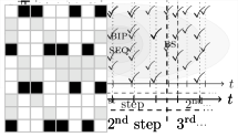
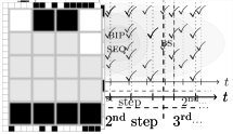
(a)   (b)   (c)   (d)   (e)

Figure 4: Space-time diagrams (time going downward) of configuration $0000001100000001$ following rule $156$ depending on: (a) the parallel update mode $\mu_{\textsc{par}}=(\llbracket 16\rrbracket)$, (b) the bipartite update mode $\mu_{\textsc{bip}}=(\{i\in\llbracket 16\rrbracket\mid i\equiv 0\mod 2\},\{i\in\llbracket 16\rrbracket\mid i\equiv 1\mod 2\})$, (c) the block-sequential update mode $\mu_{\textsc{bs}}=(\{10,15\},\{0,1,5,7,8,12\},\{4,6,9,11,14\},\{3,13\},\{2\})$, (d) the block-parallel update mode $\mu_{\textsc{bp}}=\{(0,1),(2,3,4),(5),(6,8,7),(11,10,9),(14,13,12),(15)\}$, (e) the local clocks update mode $\mu_{\textsc{lc}}=(P=(2,2,2,2,4,4,4,4,3,3,3,3,1,4,1,1),\Delta=(1,1,1,0,3,3,3,2,1,1,1,0,0,3,0,0))$.

Lemma 1

ECA rule $156$ admits only one wall, namely the word $w=01$.

Proof

For all $a,b\in\mathbb{B}$, $f_{156}(a01)=0$ and $f_{156}(01b)=1$. By definition of the rule, no other word of length $2$ gets this property. Thus $w$ is the unique wall for ECA rule $156$. ∎

Lemma 2

ECA rule $156$ can dynamically create new walls only if the underlying update mode makes two consecutive cells update their state simultaneously.

Proof

Remark that to create walls in the trajectory of a configuration $x\in\mathbb{B}^{n}$, $x$ need to have at least one wall. Indeed, the only configurations with no walls are $0^{n}$ and $1^{n}$, and they are fixed points. Thus, with no loss of generality, let us focus on a subconfiguration $y\in\mathbb{B}^{k}$, with $k\leq n-2$, composed of free state cells surrounded by two walls. Notice that since the configurations are toric, the wall “at the left” and “at the right” of $y$ can be represented by the same two cells.

Configuration $y$ is necessarily of the form $y=(1)^{\ell}(0)^{r}$, with $k=\ell+r$. Furthermore, since $f_{156}(000)=0$ and $f_{156}(100)=1$, the only cells whose states can change are those where $1$ meets $0$, i.e. $y_{\ell-1}$ and $y_{\ell}$. Such state changes depends on the schedule of updates between these two cells. Let us proceed with case disjunction:

1. Case of $\ell\geq 1$ and $r\geq 1$:

   • if $y_{\ell}$ is updated strictly before $y_{\ell-1}$, then $y^{1}=(1)^{\ell+1}(0)^{r-1}$, and the number of $1$s (resp. $0$s) increases (resp. decreases);

   • if $y_{\ell}$ is updated strictly after $y_{\ell-1}$, then $y^{1}=(1)^{\ell-1}(0)^{r+1}$, and the number of $1$s (resp. $0$s) decreases (resp. increases);

   • if $y_{\ell}$ and $y_{\ell-1}$ are updated simultaneously, then $y^{1}=(1)^{\ell-1}(01)(0)^{r-1}$, and a wall is created.

2. Case of $\ell=0$ (or of $y=0^{k}$): nothing happens until $y_{0}$ is updated. Let us admit that this first state change has been done for the sake of clarity and focus on $y^{1}=(1)^{\ell=1}(0)^{r=k-1}$, which falls into Case 1.

3. Case of $r=0$ (or of $y=1^{k}$): symmetrically to Case 2, nothing happens until $y_{k-1}$ is updated. Let us admit that this first state change has been done for the sake of clarity and focus on $y^{1}=(1)^{\ell=k-1}(0)^{1}$, which falls into Case 1.

As a consequence, updating two consecutive cells simultaneously is a necessary condition for creating new walls in the dynamics of ECA rule $156$.∎

Theorem 1

$(156,\textsc{par}{})$ has only fixed points and limit cycles of length two.

Proof

We base the proof on Lemmas 1 and 2. So, let us analyze the possible behaviors between two walls, since by definition, what happens between two walls is independent of what happens between two other walls.

Let us prove the results by considering the three possible distinct cases for a configuration between two walls $y\in\mathbb{B}^{k+4}$:

• Consider $y=(01)(0)^{k}(01)$ the configuration with only $0$s between the two walls. Applying the rule twice, we obtain $y^{2}=(01)^{2}(0)^{k-2}(01)$. So, a new wall appears every two iterations so that, for all $t<\frac{k}{2}$, $y^{2t}=(01)^{t+1}(0)^{k-2t}(01)$, until a step is reached where there is no room for more walls. This step is reached after $k$ (resp $k-1$) iterations when $k$ is even (resp. odd) and is such that there is only walls if $k$ is even (which implies that the dynamics has converged to a fixed point), and only walls except one cell otherwise. In this case, considering that $t=\lfloor\frac{k}{2}\rfloor$, because $f_{156}(100)=1$ and $f_{156}(110)=0$, we have that $y^{2t}=(01)^{t+1}(0)(01)\to y^{2t+1}=(01)^{t+1}(1)(01)\to y^{2t}=(01)^{t+1}(0)(01)$, which leads to a limit cycle of length $2$.

• Consider now that $y=(01)(1)^{k}(01)$. Symmetrically, for all $t<\frac{k}{2}$, $y^{2t}=(01)(0)^{k-2t}(01)^{t+1}$. The same reasoning applies to conclude that the length of the largest limit cycle is $2$.

• Consider finally configuration $y=(01)(1)^{\ell}(0)^{r}(01)$ for which $k=\ell+r$. Applying $f_{156}$ on it leads to $y^{1}=(01)(1)^{\ell-1}(01)(0)^{r-1}(01)$, which falls into the two previous cases. ∎

Theorem 2

$(156,\textsc{bip}{})$ of size $n$ has largest limit cycles of length $\Theta(2^{\sqrt{n\log(n)}})$.

Proof

First, by definition of a bipartite update mode and by Lemmas 1 and 2, the only walls appearing in the dynamics are the ones present in the initial configuration. Let us prove that, given two walls $u$ and $v$, distanced by $k$ cells, the largestlimit cycles of the dynamics between $u$ and $v$ are of length $k+1$. We proceed by case disjunction depending on the nature of the subconfiguration $y\in\mathbb{B}^{k+4}$, with the bipartite update mode $\mu=(\{i\in\llbracket k+4\rrbracket\mid i\equiv 0\mod 2\},\{i\in\llbracket k+4\rrbracket\mid i\equiv 0\mod 2\})$:

1. Case of $y=(01)(0)^{k}(01)$: we prove that configuration $(01)(1)^{k}(01)$ is reached after $\lceil\frac{k}{2}+1\rceil$ steps:

   • If $k$ is odd, we have:
     

     $$\begin{array}[]{ccc}y&=&(01)(0)^{k}(01)\\ y^{1}&=&(01)(1)(0)^{k-1}(01)\\ y^{2}&=&(01)111(0)^{k-3}(01)\\ &\vdots&\\ y^{\lfloor\frac{k}{2}\rfloor}&=&(01)(1)^{k-2}(00)(01)\\ y^{\lceil\frac{k}{2}\rceil}&=&(01)(1)^{k}(01)\\ \end{array}$$

   • If $k$ is even, we have:
     

     $$\begin{array}[]{ccc}y&=&(01)(0)^{k}(01)\\ y^{1}&=&(01)(1)(0)^{k-1}(01)\\ y^{2}&=&(01)(111)(0)^{k-2}(01)\\ &\vdots&\\ y^{\frac{k}{2}}&=&(01)(1)^{k-1}(0)(01)\\ y^{\frac{k}{2}+1}&=&(01)(1)^{k}(01)\\ \end{array}$$

2. Case of $y=(01)(1)^{k}(01)$: we prove that configuration $(01)(0)^{k}(01)$ is reached after $\lceil\frac{k}{2}+1\rceil$ steps:
   • If $k$ is odd, we have:
   $$\begin{array}[]{ccc}y&=&(01)(1)^{k}(01)\\ y^{1}&=&(01)(1)^{k-1}(0)(01)\\ y^{2}&=&(01)(1)^{k-3}(000)(01)\\ &\vdots&\\ y^{\lfloor\frac{k}{2}\rfloor}&=&(01)(11)(0)^{k-2}(01)\\ y^{\lceil\frac{k}{2}\rceil}&=&(01)(0)^{k}(01)\\ \end{array}$$   • If $k$ is even, we have:
   $$\begin{array}[]{ccc}y&=&(01)(1)^{k}(01)\\ y^{1}&=&(01)(1)^{k-2}(00)(01)\\ y^{2}&=&(01)(1)^{k-4}(0000)(01)\\ &\vdots&\\ y^{\frac{k}{2}}&=&(01)(11)(0)^{k-2}(01)\\ y^{\frac{k}{2}+1}&=&(01)(0)^{k}(01)\\ \end{array}$$

3. Case of $y=(01)(1)^{\ell}(0)^{r}(01)$: this case is included in Cases 1 and 2.

As a consequence, the dynamics of any $y$ leads indeed to a limit cycle of length $k+1$. Remark that if we had chosen the other bipartite update mode as reference, the dynamics of any $y$ would have been symmetric and led to the same limit cycle.

Finally, since the dynamics between two pairs of distinct walls of independent of each other, the asymptotic dynamics of a global configuration $x$ such that $x=(01)(0)^{k_{1}}(01)(0)^{k_{2}}(01)\dots(01)(0)^{k_{m}}$ is a limit cycle whose length equals to the least common multiple of the lengths of all limit cycles of the subconfigurations $(01)(0)^{k_{1}}(01),(01)(0)^{k_{2}}(01),\dots,(01)(0)^{k_{m}}(01)$. We derive that the largest limit cycles are obtained when the $(k_{i}+1)$s are distinct primes whose sum is equal to $n-2m$, with $m$ is constant. As a consequence, the length of the largest limit cycle is lower- and upper- bounded by the primorial of $n$ (i.e. the maximal product of distinct primes whose sum is $\leq n$.), denoted by function $h(n)$. In [5], it is shown in Theorem $18$ that when $n$ tends to infinity, $\log h(n)\sim\sqrt{n\log n}$. Hence, we deduce that the length of the largest limit cycles of $(156,\textsc{bip}{})$ of size $n$ is $\Theta(2^{\sqrt{n\log(n)}})$. ∎

Corollary 1

The families $(156,\textsc{bs}{})$, $(156,\textsc{bp}{})$ and $(156,\textsc{lc}{})$ of size $n$ have largest limit cycles of length $\Omega(2^{\sqrt{n\log(n)}})$.

Proof

Since the bipartite update modes are specific block-sequential and block-parallel update modes, and since both block-sequential and block-parallel update modes are parts of local-clocks update modes, all of them inherit the property stating that the lengths of the largest limit cycles are lower-bounded by $2^{\sqrt{n\log(n)}}$. ∎

3.2 ECA rule $178$

ECA rule $178$ is defined locally by the following transition table:

$\begin{array}[]{|c||c|c|c|c|c|c|c|c|}\hline\cr(x_{i-1}^{t},x_{i}^{t},x_{i+1}^{t})&000&001&010&011&100&101&110&111\\ \hline\cr x_{i}^{t+1}&0&1&0&0&1&1&0&1\\ \hline\cr\end{array}$

Space-time diagrams depending on different update modes of a specific configuration under ECA rule $178$ are given in Figure 5. Each of them depict trajectories giving ideas of how to reach a limit cycle of high complexity.

       

(a)   (b)   (c)   (d)   (e)

Figure 5: Space-time diagrams (time going downward) of configuration $0000011010111110$ following rule $178$ depending on: (a) the parallel update mode $\mu_{\textsc{par}}=(\llbracket 16\rrbracket)$, (b) the bipartite update mode $\mu_{\textsc{bip}}=(\{i\in\llbracket 16\rrbracket\mid i\equiv 0\mod 2\},\{i\in\llbracket 16\rrbracket\mid i\equiv 1\mod 2\})$, (c) the block-sequential update mode $\mu_{\textsc{bs}}=(\{3,9,15\},\{2,4,8,10,14\},\{11,5,7,11,13\},\{0,6,12\})$, (d) the block-parallel update mode $\mu_{\textsc{bp}}=\{(0),(1),(2,3),(4,5),(6),(7),(8),(9),(10,11),(12,13),(14,15)\}$, (e) the local clocks update mode $\mu_{\textsc{lc}}=(P=(1,1,2,2,2,2,1,1,1,4,4,4,4,4,4,4),\Delta=(0,0,1,0,1,0,0,0,0,0,1,0,1,0,1,0))$.

Lemma 3

ECA rule $178$ admits two walls, $01$ and $10$, which are relative walls.

Proof

Let $a,b\in\mathbb{B}$. Notice that by definition of the rule: $f(a00)\neq f(b00)$ and $f(00a)\neq f(00b)$, and $f(a11)\neq f(b11)$ and $f(11a)\neq f(11b)$ if $a\neq b$; $f(a01)=1$ and $f(01a)=0$; and $f(a10)=0$ and $((10a)=1$. Thus, neither $00$ nor $01$ nor $10$ nor $11$ are absolute walls. From what precedes, notice that the properties of $00$ and $11$ prevent them to be relative walls. Consider now the two words $u=01$ and $v=10$ and let us show that they constitute relative walls. Regardless the states of the cells surrounding $u$, every time both cells of $u$ are updated simultaneously, $u$ changes to $v$ and similarly, $v$ will change to $u$ independently of the states of the cells that surround it, as long as both its cells are updated together. Thus, $u$ and $v$ are relative walls. ∎

We will show certain bp and lc update modes that are able to produce these relative walls.

Theorem 3

Each representative of $(178,\textsc{bip}{})$ of size $n$ has largest limit cycles of length $\Theta(n)$.

Proof

By Lemma 3 (and its proof), $(178,\textsc{bip}{})$ has no walls since there is no way of updating two consecutive cells simultaneously. Since configurations $0^{n}$ and $1^{n}$ are fixed points, let us consider other configurations and denote by $\mu_{\textsc{bip}}{}$ (resp. $\overline{\mu}_{\textsc{bip}}{}$) the update mode defined by $(\{i\in\llbracket n\rrbracket\mid i\equiv 0\mod 2\},\{i\in\llbracket n\rrbracket\mid i\equiv 1\mod 2\})$ (resp. the other one). Let us begin with configurations $x$ composed by one isle $1$s. With no loss of generality, let us take $x=(1)^{\ell}(0)^{r}$, with $n=\ell+r\equiv 0\mod 2$ by definition of a bipartite update mode:

• If $\ell$ is odd, with $\mu_{\textsc{bip}}{}$, we have:

  $$\begin{array}[]{ccl}x&=&(1)^{\ell}(0)^{r}\\ x^{1}&=&(0)^{2}(1)^{\ell-4}(0)^{r+2}\\ &\vdots&\\ x^{i}&=&(0)^{2i}(1)^{\ell-4i}(0)^{r+2i}\\ &\vdots&\\ x^{\lfloor\frac{\ell}{4}\rfloor}&=&\begin{cases}(0)^{\lfloor\frac{\ell}{2}\rfloor}(1)(0)^{\lfloor\frac{\ell}{2}\rfloor}&\text{if }\ell\text{ is the smallest of the two odd numbers}\\ &\text{with equal }\lfloor\frac{\ell}{4}\rfloor\\ (0)^{\lfloor\frac{\ell}{2}\rfloor}(1)^{3}(0)^{\lfloor\frac{\ell}{2}\rfloor}&\text{otherwise}\\ \end{cases}\\ x^{\lfloor\frac{\ell}{4}\rfloor+1}&=&(0)^{n}\text{.}\end{array}$$

  With $\overline{\mu}_{\textsc{bip}}{}$, with a similar reasoning, we get the symmetric result with the number of $1$s increasing by $4$ at each step. Consequently, such configurations lead to fixed points, either $0^{n}$ or $1^{n}$.

• If $\ell$ is even, let us show that the isle of $1$s shifts over time to the right with $\mu_{\textsc{bip}}{}$ and to the left with $\overline{\mu}_{\textsc{bip}}{}$. With $\mu_{\textsc{bip}}{}$, we have:

  $$\begin{array}[]{ccl}x&=&(1)^{\ell}(0)^{r}\\ x^{1}&=&(0)(2)^{\ell}(0)^{r-2}\\ &\vdots&\\ x^{i}&=&(0)^{2i}(1)^{\ell}(0)^{r-2i}\\ &\vdots&\\ \end{array}$$

  $$\begin{array}[]{ccl}x^{\frac{n}{2}-1}&=&(1)^{\ell-2}(0)^{r}(1)^{2}\\ x^{\frac{n}{2}}&=&(1)^{\ell}(0)^{r}\text{.}\end{array}$$

  With $\overline{\mu}_{\textsc{bip}}{}$, with a similar reasoning, we get the symmetric result, the isle of $1$s shifting to the left. Consequently, such configurations lead to limit cycles of length $\frac{n}{2}$.

Now, let us consider configurations with several isles of $1$s. With no loss of generality, let us focus on configurations with two isles of $1$s because they capture all the possible behaviors. There are $10$ distinct cases which depends on both the parity of the size of the isles of $1$s and the parity of the position of the first cell of each isle. This second criterion coincides locally with the nature of the bipartite update mode. Indeed, given an isle of $1$s, if its first cell $i$ is even (resp. odd), then the isle follows $\mu_{\textsc{bip}}{}$ (resp. $\overline{\mu}_{\textsc{bip}}{}$) locally. For the sake of clarity, let us make us of the following notation: we use $\alpha\in\{\mathrm{e},\mathrm{o}\}$ to denote the parity of the size of the isles of $1$s, and $\beta\in\{\mu,\overline{\mu}\}$ to denote the local bipartite update mode followed by the isles. Let us proceed by case disjunction, where the cases are denoted by a pair of criterion of each sort, one for the first isle of $1$s, another one for the second.

• If the two isles of $1$s are of even sizes:

  1. Case $(e_{\mu},e_{\mu})$: By what precedes, because the two isles are separated by each other by an even number of cells at least equal to $2$, they both shift to the right with an index equal to $2$ over time. Thus, such a configuration lead to a limit cycle of length $\frac{n}{2}$.

  2. Case $(e_{\overline{\mu}},e_{\overline{\mu}})$: This case is similar to the previous one, except that the isles shift to the right.

  3. Case $(e_{\mu},e_{\overline{\mu}})$: By what precedes, the first isle shifts to right as well as the second isle shifts to the left over time, both with an index $2$. They do so synchronously at each time step until the isles meet. Notice that the two isles are followed by an odd number of $0$s. So, let us consider that initial configuration $x=(1)^{k}(0)^{\ell}(1)^{k^{\prime}}(0)^{r}$, with $n=k+k^{\prime}+\ell+r$. The two isles inevitably meet from a configuration $x^{t}=(1)^{k}(0)^{\ell^{\prime}}(1)^{k^{\prime}}(0)^{r^{\prime}}$ (up to rotation of the configuration on the torus), where $k,k^{\prime},\ell^{\prime},r^{\prime},t\in\mathbb{Z}$ and $n=k+k^{\prime}+\ell^{\prime}+r^{\prime}$ such that $k$ and $k^{\prime}$ are even and represent the size of each isle, $\ell^{\prime}$ and $r^{\prime}$ are odd, and $\ell^{\prime}=3$ (resp. $\ell^{\prime}=1$) if the initial number of $0$s following the first isle in $x^{0}$ is the smallest (resp. the biggest) of the odd numbers with equal $\lfloor\frac{\ell}{4}\rfloor$. Then, we have:

     $$\begin{array}[]{ccc}x^{t}&=&(1)^{k}(0)^{\ell^{\prime}}(1)^{k^{\prime}}(0)^{r^{\prime}}\\ x^{t+1}&=&(0)^{2}(1)^{k+k^{\prime}-1}(0)^{r^{\prime}+2}\text{.}\end{array}$$

     Configuration $x^{t+1}$ is then composed of a unique isle of $1$s of odd size whose first cell position is even, i.e. this isle follows $\mu_{\textsc{bip}}{}$ locally and converges to $0^{n}$ as proven above. Remark that the case $(e_{\overline{\mu}},e_{\mu})$ is strictly equivalent because of the toric nature of the ECA.

• If the two isles of $1$s are of odd sizes:

  1. Case $(o_{\mu},o_{\mu})$: By what precedes, the two isles evolve locally by decreasing their numbers of $1$s until $x$ becomes the fixed point $0^{n}$.

  2. Case $(o_{\mu},o_{\overline{\mu}})$: Notice first that by definition, the two isles are inevitably separated by even numbers $\ell\geq 2$ and $r\geq 2$ of $0$s on each side. Let us consider configuration $x=(1)^{k}(0)^{\ell}(1)^{k^{\prime}}(0)^{r}$ such that $n=k+k^{\prime}+\ell+r$. By what precedes, the first isle evolves locally towards $O^{k}$ by losing four $1$s (two from each side) at each step. Conversely, the second isle increases its number of $1$s by four (two more on each side) at each step. Consequently, these two isles of $1$s never meet and the first isle spreads it $1s$ over time until $x$ reaches $1^{n}$. Remark that the case $(o_{\overline{\mu}},o_{\mu})$ is strictly equivalent because of the toric nature of the ECA.

  3. Case $(o_{\overline{\mu}},o_{\overline{\mu}})$: By what precedes, the two isles increases by four their number of $1$s (two on each side). Inevitably, there exists a step $t$ at which they meet and become a unique isle of $1$s such that the position of its first cell position is odd, because of the parity of the increasing of $1$s, and follows thus $\overline{\mu}_{\textsc{bip}}{}$. As a consequence, this isle spreads its $1$s and $x$ evolves over time until it reaches $1^{n}$.

• If the sizes of the two isles of $1$s are of distinct parity:

  1. Case $(e_{\mu},o_{\mu})$: First, notice that configuration $x$ is necessary such that there are an even (resp. odd) number of $0$s which follow the first (resp. second) isle. So, let us consider $x=(1)^{k}(0)^{\ell}(1)^{k^{\prime}}(0)^{r}$, with $\ell\geq 2$ even and $r$ odd, such that $n=k+k^{\prime}+\ell+r$. By what precedes, the first isle shifts to the right with index $2$ at each time step. The second isle reduces its its number of $1$s by four at each step ($two$ on each side). Thus, the two isles never meet: the second isle converges locally to $0^{k^{\prime}}$ while the first isle keeps shifting with an index $2$ over time. Thus, $x$ reaches a limit cycle of length $\frac{n}{2}$.

  2. Case $(e_{\mu},o_{\overline{\mu}})$: By what precedes, the first isle dynamically shifts to the right with an index $2$ and the second increases its number of $1$s by four (two on each side) at each step. Notice that configuration $x$ is necessary such that there are an odd (resp. even) number of $0$s which follow the first (resp. second) isle. So, let us consider that initial configuration $x=(1)^{k}(0)^{\ell}(1)^{k^{\prime}}(0)^{r}$, with $n=k+k^{\prime}+\ell+r$, and $\ell$ odd and $r\geq 2$ even. The two isles inevitably meet from a configuration $x^{t}=(1)^{k}(0)^{\ell^{\prime}}(1)^{k^{\prime\prime}}(0)^{r}$ (up to rotation of the configuration on the torus), where $k,k^{\prime\prime},\ell^{\prime},r,t\in\mathbb{Z}$ and $n=k+k^{\prime\prime}+\ell^{\prime}+r$ such that $k$ and $k^{\prime\prime}$ are even and represent the size of each isle at step $t$, and $\ell^{\prime}=3$ (resp. $\ell^{\prime}=1$) if the initial number of $0$s following the first isle in $x^{0}$ is the smallest (resp. the biggest) of the odd numbers with equal $\lfloor\frac{\ell}{4}\rfloor$. Then, we have:

     $$\begin{array}[]{ccc}x^{t}&=&(1)^{k}(0)^{\ell^{\prime}}(1)^{k^{\prime\prime}}(0)^{r}\\ x^{t+1}&=&(0)^{2}(1)^{n-r}(0)^{r-2}\text{.}\end{array}$$

     Configuration $x^{t+1}$ is then composed of a unique isle of $1$s of even size whose first cell position is even, i.e. this isle follows $\mu_{\textsc{bip}}{}$ locally, and shifts to the right with index $2$. Thus, $x$ reaches a limit cycle of length $\frac{n}{2}$.

  3. Case $(e_{\overline{\mu}},o_{\mu})$: Applying on this case the same reasoning as in the case $(e_{\mu},o_{\mu})$ allows to show a dynamics which is symmetric, in the sense that such a configuration evolves asymptotically towards a limit cycle characterized by the first isle of $1$s shifting to the left with index $2$, which confirms the reachability of a limit cycle of length $\frac{n}{2}$.

  4. Case $(e_{\overline{\mu}},o_{\overline{\mu}})$: Applying on this case the same reasoning as in the case $(e_{\mu},o_{\overline{\mu}})$ allows to show a dynamics which symmetric, in the sense that such a configuration evolves asymptotically towards a limit cycle characterized by a unique isle of $1$s of size $n-\ell$ shifting to the left with index $2$, which confirms the reachability of a limit cycle of length $\frac{n}{2}$.

All these cases taken together show that the largest limit cycle reachable by $(178,\textsc{bip}{})$ is of length $\frac{k}{2}=O(n)$. ∎

Theorem 4

The family $(178,\textsc{bp})$ of size $n$ has largest limit cycles of length $\Omega\left(2^{\sqrt{n\log n}}\right)$

Proof

Notice that the configurations of interest here are those having at least one relative wall since $(0)^{n}$ and $(1)^{n}$ are fixed points. By Lemma 3 (and its proof) $w_{1}$ and $w_{2}$ are relative walls for the family $(178,\textsc{bp})$ since there exist block-parallel updates modes guaranteeing that the two contiguous cells carrying $w_{1}$ (resp. $w_{2}$) are updated simultaneously and an even number of substeps over the period. Thus, let us consider in this proof an initial configuration $x$ with at least one wall. The idea is to focus on what can happen between two walls because the dynamics of two subconfigurations delimited by two distinct pairs of walls are independent from each other.

Now, let $y$ (resp. $y^{\prime}$) be a subconfiguration of size $k+4$ such that $y=(w_{\ell},y_{2},\dots,y_{k+1},w_{r})$, with $w_{\ell}=y_{0}y_{1},w_{r}=y_{k+2}y_{k+3}$ two relative walls in $W=\{w_{1},w_{2}\}$ and such that for all $i\in\{2,\dots,k+1\},y_{i}=0$ (resp. $y_{i}^{\prime}=1$) and the block-parallel mode

$$\begin{split}\mu_{\textsc{bp}}&=\{(y_{0}),(y_{1}),(y_{2},y_{3}),\dots,(y_{k},y_{k+1}),(y_{k+2}),(y_{k+3})\}\\ &\equiv(\{y_{0},y_{1},y_{2},y_{4},\dots,y_{k},y_{k+2},y_{k+3}\},\{y_{0},y_{1},y_{3},y_{5},\dots,y_{k+1},y_{k+2},y_{k+3}\}),\end{split}$$

if $k$ is even, and:

$$\begin{split}\mu_{\textsc{bp}}&=\{(y_{0}),(y_{1}),(y_{2},y_{3}),\dots,(y_{k},y_{k+1}),(y_{k+2}),(y_{k+3})\}\\ &\equiv(\{y_{0},y_{1},y_{2},y_{4},\dots,y_{k+1},y_{k+2},y_{k+3}\},\{y_{0},y_{1},y_{3},y_{5},\dots,y_{k},y_{k+2},y_{k+3}\}),\end{split}$$

if $k$ is odd.

The dynamics of $y$ follows four cases:

1. $w_{\ell}=w_{r}=01$, given $\tau\in\mathbb{Z}$, denoting the subconfigurations obtained at a substep by $y^{\frac{\tau}{2}}$:

   – If $k$ is even, we have

   $$y = (01)(0)^{k}(01)$$

   $$y^{\left(\frac{1}{2}\right)} = (10)(1)(0)^{k-1}(10)$$

   $$y^{1} = (01)(1)^{2}(0)^{k-3}(1)(01)$$

   $$y^{\left(\frac{3}{2}\right)} = (10)(1)^{3}(0)^{k-5}(1)^{2}(10)$$

   $$y^{2} = (01)(1)^{4}(0)^{k-7}(1)^{3}(01)$$

   $$\vdots$$

   $$y^{i} = (01)(1)^{2i}(0)^{k-4i+1}(1)^{2i-1}(01)$$

   $$\vdots$$

   $$y^{\frac{k-1}{2}} = (01)(1)^{k}(01)$$

   $$y^{\frac{k}{2}-1} = (10)(1)^{k}(10)$$

   $$y^{\frac{k}{2}} = (01)(1)^{k}(01)$$

   – If $k$ is odd, we have

   $$y = (01)(0)^{k}(01)$$

   $$y^{\left(\frac{1}{2}\right)} = (10)(1)(0)^{k-1}(10)$$

   $$y^{1} = (01)(1)^{2}(0)^{k-2}(01)$$

   $$\vdots$$

   $$y^{i} = (01)(1)^{2i}(0)^{k-2i}(01)$$

   $$\vdots$$

   $$y^{\frac{k+1}{2}} = (01)(1)^{k}(01)$$

   $$y^{\frac{k+2}{2}} = (10)(1)^{k-1}(0)(10)$$

   $$y^{\frac{k+3}{2}} = (01)(1)^{k-2}(0)^{2}(01)$$

   $$\vdots$$

   $$y^{k+1} = (01)(0)^{k}(01)$$

   Thus, subconfiguration $y$ converges towards fixed point $(01)(1)^{k}(01)$ when $k$ is even and leads to a limit cycle of length $k+1$ when $k$ is odd.

2. $w_{\ell}=w_{r}=10$: taking $y^{\prime}$ as the initial subconfiguration, and applying the same reasoning, we can show that this case is analogous to the previous one up to a symmetry, which allows us to conclude that $y^{\prime}$ converges towards fixed point $(10)(0)^{k}(10)$ when $k$ is even and leads to a limit cycle of length $k+1$ when $k$ is odd.

3. $w_{\ell}=01$ and $w_{r}=10$:
   – If $k$ is even, we have $\displaystyle y$ $\displaystyle=$ $\displaystyle(01)(0)^{k}(10)$ $\displaystyle y^{\left(\frac{1}{2}\right)}$ $\displaystyle=$ $\displaystyle(10)(1)(0)^{k-1}(01)$ $\displaystyle y^{1}$ $\displaystyle=$ $\displaystyle(01)(1)^{2}(0)^{k-2}(10)$ $\displaystyle\vdots$ $\displaystyle y^{i}$ $\displaystyle=$ $\displaystyle(01)(1)^{2i}(0)^{k-2i}(10)$ $\displaystyle\vdots$ $\displaystyle y^{\frac{k}{2}}$ $\displaystyle=$ $\displaystyle(01)(1)^{k}(10)$ $\displaystyle y^{\left(\frac{k+1}{2}\right)}$ $\displaystyle=$ $\displaystyle(10)(1)^{k}(01)$ $\displaystyle y^{\left(\frac{k+2}{2}\right)}$ $\displaystyle=$ $\displaystyle(01)(1)^{k-1}(0)(10)$ $\displaystyle\vdots$ $\displaystyle y^{k+1}$ $\displaystyle=$ $\displaystyle(01)(0)^{k}(10)$ – If $k$ is odd, we have $\displaystyle y$ $\displaystyle=$ $\displaystyle(01)(0)^{k}(10)$ $\displaystyle y^{\left(\frac{1}{2}\right)}$ $\displaystyle=$ $\displaystyle(10)(1)(0)^{k-2}(01)$ $\displaystyle y^{1}$ $\displaystyle=$ $\displaystyle(01)(1)^{2}(0)^{k-4}(1)^{2}(10)$ $\displaystyle y^{\left(\frac{3}{2}\right)}$ $\displaystyle=$ $\displaystyle(10)(1)^{3}(0)^{k-6}(1)^{3}(01)$ $\displaystyle y^{2}$ $\displaystyle=$ $\displaystyle(01)(1)^{4}(0)^{k-8}(1)^{4}(01)$ $\displaystyle\vdots$ $\displaystyle y^{i}$ $\displaystyle=$ $\displaystyle(01)(1)^{2i}(0)^{k-4i}(1)^{2i}(10)$ $\displaystyle\vdots$ $\displaystyle y^{\left(\frac{k-1}{2}\right)}$ $\displaystyle=$ $\displaystyle(01)(1)^{k}(10)$ $\displaystyle y^{\frac{k}{2}}$ $\displaystyle=$ $\displaystyle(10)(1)^{k}(01)$ $\displaystyle y^{\frac{k+1}{2}}$ $\displaystyle=$ $\displaystyle(01)(1)^{k}(10)$ Thus, subconfiguration $y$ leads to a limit cycle of length $k+1$ when $k$ is even and converges towards fixed point $(01)(1)^{k}(10)$ when $k$ is odd.

4. $w_{\ell}=10$ and $w_{r}=10$: taking $y^{\prime}$ as the initial subconfiguration, and applying the same reasoning we can show that this case is analogous to the previous one up to a symmetry, which allows us to conclude that $y^{\prime}$ leads to a limit cycle of length $k+1$ when $k$ is even and converges towards fixed point $(10)(0)^{k}(01)$ when $k$ is odd.

Since the dynamics between two pairs of distinct walls is independent of each other, the asymptotic dynamics of a global configuration $x$ is a limit cycle whose length equals the least common multiple of the lengths of all limit cycles of the subconfigurations embedded into pairs of walls. With the same argument as the one used in the proof of Theorem 2, we derive that the length of the largest limit cycles of the family $(178,\textsc{bp})$ applied over a grid of size $n$ is $\Omega\left(2^{\sqrt{n\log n}}\right)$. ∎

Theorem 5

$(178,\textsc{seq})$ of size $n$ has largest limit cycles of length $O(n)$.

Proof

Let us fix $n\in\mathbb{N}$ and let us call $f$ the $178$-ECA rule. Let us also fix a sequential update mode $\mu$. We recall the notation $\mu(n)=\mu_{n}\in\llbracket n\rrbracket$ to denote the node that will be updated at time $t=n$. We will refer to the global rule under the update mode $\mu$ as $F$.

First, observe that, for the rule $178$, since $f(000)=0$ and $f(111)=1$ then, the configurations $1^{*}$ and $0^{*}$ are fixed points for the parallel update mode. Thus, we have that they are also fixed points for the sequential update modes, i.e $f_{\mu_{n}}(111)=1$ and $f_{\mu_{n}}(000)=0$ for all $n\in\mathbb{N}$ and $F_{178}(1^{*})=1^{*},F_{178}(0^{*})=0^{*}$.

Let us consider an interval $I_{0}=[p,q]\subseteq\llbracket n\rrbracket$ and a configuration $x$ such that $x_{i}=1$ for all $i\in I_{0}$ and $x_{i}=0$ otherwise. We distinguish four different cases depending on the update mode:

1. Cell $p-1$ updates before $p$ (formally $\mu_{p-1}<\mu_{p}$), and $q+1$ before $q$ ($\mu_{q}>\mu_{q+1}$).

   In that case, we have a situation as the one illustrated in the following table:

   $\dots$	$p-2$	$p-1$	$p$	$p+1$	$\dots$	$q-1$	$q$	$q+1$	$q+2$	$\dots$
   $\dots$	$0$	$0$	$1$	$1$	$\dots$	$1$	$1$	$0$	$0$	$\dots$
   $\dots$	$0$	$1$	$1$	$1$	$\dots$	$1$	$1$	$1$	$0$	$\dots$

   We will prove by induction that in this case the state of every cell of the configuration is $1$ after a finite number of steps. Since the patterns $001$ and $100$ are such that $f(001)=1$ and $f(100)=1$ then, we have that the nodes $p-1$ and $q+1$ will change their states to $1$. Let us define $\ell_{1}=\max\{i<p:\mu_{i-1}<\mu_{i}\ \wedge\ \mu_{i}>\mu_{i+1}\}$ and $r_{1}=\min\{i>q:\mu_{i-1}<\mu_{i}\ \wedge\ \mu_{i}>\mu_{i+1}\}$, and consider $L_{1}=[\ell_{1},p-1]$ and $R_{1}=[q+1,r_{1}]$.

   $\ell-1$	$\ell$	$\dots$	$p-1$	$p$	$\dots$	$q$	$q+1$	$\dots$	$r$	$r+1$
   $0$	$0$	$\dots$	$0$	$1$	$\dots$	$1$	$0$	$\dots$	$0$	$0$
   $0$	$1$	$\dots$	$1$	$1$	$\dots$	$1$	$1$	$\dots$	$1$	$0$

   We have that $F(x)=y$ where for $y$, there exists an interval $I_{1}=L_{1}\cup I_{0}\cup R_{1}$ such that $I_{0}\subseteq I_{1}$ and that $y_{i}=1$ for all $i\in I_{1}$ and $y_{i}=0$ otherwise. In addition, because of the assumptions of this case, we have that the inclusion is strict, i.e. $|I_{1}|>|I_{0}|$, and that $\mu_{\ell_{1}-1}<\mu_{\ell_{1}}$ and $\mu_{r}>\mu_{r+1}$.

   Now, we are going to show that for each $k\geq 1$, there exists a sequence of intervals $I_{1},\ldots,I_{k}$ such that $I_{1}\subseteq I_{2}\subseteq\ldots\subseteq I_{k}$, $|I_{1}|<\ldots<|I_{k}|$, and such that for each $k\in\llbracket n\rrbracket$, we have that:

   1. $I_{k}=[\ell_{k},r_{k}]$

   2. $I_{0}\subsetneq I_{1}\subsetneq\dots\subsetneq I_{k}$.

   We proceed by induction. For $k=1$, the base case is given by the latter construction. Now assume that there exists a sequence of $I_{k}$ such that they have properties (a) and (b). Then, let us define $\ell_{k+1}=\max\{i<\ell_{k}:\mu_{i-1}<\mu_{i}\ \wedge\ \mu_{i}>\mu_{i+1}\}$ and $r_{k+1}=\min\{i>r_{k}:\mu_{i-1}<\mu_{i}\ \wedge\ \mu_{i}>\mu_{i+1}\}$. Both $\ell_{k+1}$ and $r_{k+1}$ are well defined because if $\mu_{\ell_{k}-1}<\mu_{\ell_{k}}$, then $\ell_{k+1}=\ell_{k}-1$ and, similarly, if $\mu_{r_{k}}>\mu_{r_{k}+1}$, then $r_{k+1}=r_{k}+1$. From there, we can define $L_{k+1}=[\ell_{k+1},\ell_{k}-1]$ and $R_{k+1}=[r_{k}+1,r_{k+1}]$. Indeed, if $I_{k+1}=R_{k+1}\cup I_{k}\cup L_{k+1}$, then $I_{k+1}=[\ell_{k+1},r_{k+1}]$, and $I_{k}\subsetneq I_{k+1}$. And because $|I_{k}|<|I_{k+1}|$ after $t$ iterations of $F_{178}$ ($t<n$), the configuration reaches an homogeneous fixed point in which the state of each cell will be equal to $1$, i.e. $F_{178}^{t}(x)=1^{*}$.

2. $\mu_{p-1}>\mu_{p}$ and $\mu_{q}<\mu_{q+1}$. This case is similar to Case 1, considering an isle of $0$s surrounded by $1$s.

   $\dots$	$p-2$	$p-1$	$p$	$p+1$	$\dots$	$q-1$	$q$	$q+1$	$q+2$	$\dots$
   $\dots$	$0$	$0$	$1$	$1$	$\dots$	$1$	$1$	$0$	$0$	$\dots$
   $\dots$	$0$	$0$	$0$	$1$	$\dots$	$1$	$0$	$0$	$0$	$\dots$

   This means that Case 2 leads always to the homogeneous fixed point $0^{n}$.

3. $\mu_{p-1}>\mu_{p}$ and $\mu_{q}>\mu_{q+1}$.

   $\dots$	$p-2$	$p-1$	$p$	$p+1$	$\dots$	$q-1$	$q$	$q+1$	$q+2$	$\dots$
   $\dots$	$0$	$0$	$1$	$1$	$\dots$	$1$	$1$	$0$	$0$	$\dots$
   $\dots$	$0$	$0$	$0$	$1$	$\dots$	$1$	$1$	$1$	$0$	$\dots$

   According to the analysis made for Case 1, we know that the configuration gains $1$s to the right of the isle until it reaches a cell that we call $r$. We need to find how the dynamics will behave to the left.

   If $p+1$ updates after $p$ ($\mu_{p}<\mu_{p+1}$), then cell $p+1$ will become $0$. Thus, let $r_{1}^{\prime}\in\mathbb{N}$ be such that $r_{1}^{\prime}=\min\{s>p:\mu_{i-1}<\mu_{i}\ \wedge\ \mu_{i}>\mu_{i+1}\}$. Then, we will lose $1$s until we reach cell $r^{\prime}$.

   $p-1$	$p$	$p+1$	$\dots$	$r^{\prime}$	$r^{\prime}+1$	$\dots$	$q$	$q+1$	$\dots$	$r$	$r+1$
   $0$	$1$	$1$	$\dots$	$1$	$1$	$\dots$	$1$	$0$	$\dots$	$0$	$0$
   $0$	$0$	$0$	$\dots$	$0$	$1$	$\dots$	$1$	$1$	$\dots$	$1$	$0$

   Note that both $r_{1}$ and $r_{1}^{\prime}$ are defined by the fact that they update after the cell to their right ($\mu_{r_{1}}>\mu_{r_{1}+1}$ and $\mu_{r_{1}^{\prime}}>\mu_{r_{1}^{\prime}+1}$). Similarly, we can define $p_{1}=r_{1}^{\prime}+1$ and $q_{1}=r_{1}$, and in turn, find new $r^{\prime}_{2}$ and $r_{2}$ defined by $r_{2}^{\prime}=\min\{s>r_{1}^{\prime}:\mu_{s-1}<\mu_{s}\ \wedge\ \mu_{s}>\mu_{s+1}\}$ and $r_{1}=\min\{s>r_{1}:\mu_{s-1}<\mu_{s}\ \wedge\ \mu_{s}>\mu_{s+1}\}$. Recursively, we define $r_{k}^{\prime}=\min\{s>r_{k-1}^{\prime}:\mu_{s-1}<\mu_{s}\ \wedge\ \mu_{s}>\mu_{s+1}\}$ and $r_{k}=\min\{s>r_{k-1}:\mu_{s-1}<\mu_{s}\ \wedge\ \mu_{s}>\mu_{s+1}\}$ and since by definition, $\mu_{r_{i}^{\prime}}>\mu_{r_{i}^{\prime}+1}$ and $\mu_{r_{i}}>\mu_{r_{i}+1}$, we conclude that the isle of $1$s shifts over time to the right, and because the configuration is a ring, this gives rise to a cycle.

4. $\mu_{p-1}<\mu_{p}$ and $\mu_{q}<\mu_{q+1}$. This case is similar to Case 3, except that the isle of $1$s shifts over time to the left.

Now, let us denote by $\{r_{i}\}_{i=1}^{N}$, with $N\in\llbracket n\rrbracket$, the set of cells such that $\mu_{r_{i}}>\mu_{r_{i}+1}$). Using these $r_{i}$, we can partition the ring into sections from cell $r_{i}+1$ to cell $r_{i+1}$, as shown on the following table:

$\dots$

$r_{i-1}$

$r_{i-1}+1$

$\dots$

$r_{i}$

$r_{i}+1$

$\dots$

$r_{i+1}$

$r_{i+1}+1$

$\dots$

If the isle of $1$s starts on a cell $p\not\in\{r_{l}\}_{l=1}^{N}$ for all $i\in\{1,\dots,N\}$, and ends on a cell $q\in\{r_{l}\}_{l=1}^{N}$, then we are in Case 1, and this situation can only lead to a homogeneous fixed point. If the isle starts on a cell $p\in\{r_{l}\}_{l=1}^{N}$, and ends on a cell $q\not\in\{r_{l}\}_{l=1}^{N}$, then we are in Case 2, which also leads to a homogeneous fixed point. If there exists $r_{i},r_{j}\in\{r_{l}\}_{l=1}^{N}$ such that $p=r_{i}+1$ and $q=r_{j}$, with $1\leq i<j\leq N$, then we are on Case 3, and it leads to a cycle. As seen in Case 3, we know that we gain $1$s to the right until we reach from cell $r_{j}$ to cell $r_{j+1}$. Similarly, we know that we lose $1$s from cell $r_{i}+1$ to cell $r_{i+1}+1$, as shown on the following graphic.

$\dots$	$r_{i}$	$r_{i}+1$	$\dots$	$r_{i+1}$	$r_{i+1}+1$	$\dots$	$r_{j}$	$r_{j}+1$	$\dots$	$r_{j+1}$	$r_{j+1}+1$	$\dots$
$\dots$	$0$	$1$	$\dots$	$1$	$1$	$\dots$	$1$	$0$	$\dots$	$0$	$0$	$\dots$
$\dots$	$0$	$0$	$\dots$	$0$	$1$	$\dots$	$1$	$1$	$\dots$	$1$	$0$	$\dots$

It is not difficult to see that after $N-j$ iterations, the isle of $1$s will have to start on $r_{i*}+1$, with $i*=i+N-j$, and to end on $r_{N}$ ($N=j+(N-j)$). Since we are working on a ring, the section after $r_{N}$ goes from $r_{N}+1$ to $r_{1}$, meaning that at the $N-j+1$ iteration, the isle of $1$s starts on $r_{i*+1}$ and ends on $r_{1}$. $j-1$ iterations after that, the isle will go from $r_{i}+1$ to $r_{j}$, completing the cycle ($i=i+(N-j)+1+(j-1)$ and $j=j+(N-j)+1+(j-1)$), meaning that it takes $(N-j)+1+(j-1)=N$ iterations to complete the cycle.

Observe that, until here, we have been working with a single isle of $1$s. Let us assume now that the configuration has two isles of $1$s and let us denote them by $B_{1}$ and $B_{2}$). Consider the following proof based on a case disjunction:

1. Let us assume that there are $i,j,k\in\{1,\dots,N\}$ such that $B_{1}$ starts on $r_{i}+1$ and ends on $r_{j}$, while $B_{2}$ starts on $r_{k}+1$ and ends on $q\not\in\{r_{l}\}_{l=1}^{N}$. Because there are two isles, we know that $1\leq i<j<k\leq N$.

   $\dots$

   $r_{i}$

   $r_{i}+1$

   $\dots$

   $r_{j}$

   $r_{j}+1$

   $\dots$

   $r_{k}$

   $r_{k}+1$

   $\dots$

   $q$

   $q+1$

   $\dots$

   $\dots$

   $0$

   $1$

   $\dots$

   $1$

   $0$

   $\dots$

   $0$

   $1$

   $\dots$

   $1$

   $0$

   $\dots$

   Since with each iteration $B_{1}$ can only gain $1$s up to the next cell such that $\mu_{r}>\mu_{r+1}$, this means that at most

   $$r_{j+1}=r_{k}<r_{k+1}\implies r_{j+t}=r_{k+t-1}<r_{k+t}\text{.}$$

   This means that the two isles of $1$s stay separated. Moreover, since $q\not\in\{r_{l}\}_{l=1}^{N}$ then $B_{2}$ will also lose $1$s to the right. This means that $B_{2}$ will disappear without interacting with $B_{1}$.
   The case with $i,j,k\in\{1,\dots,N\}$ such that $B_{2}$ starts on $r_{i}+1$ and ends on $r_{j}$, while $B_{1}$ starts on $r_{k}+1$ but ends on $q\not\in\{r_{l}\}_{l=1}^{N}$ is similar.

   $\dots$

   $r_{k}$

   $r_{k}+1$

   $\dots$

   $q$

   $q+1$

   $\dots$

   $r_{i}$

   $r_{i}+1$

   $\dots$

   $r_{j}$

   $r_{j}+1$

   $\dots$

   $\dots$

   $0$

   $1$

   $\dots$

   $1$

   $0$

   $\dots$

   $0$

   $1$

   $\dots$

   $1$

   $0$

   $\dots$

2. Let us assume that there are $i,j,k\in\{1,\dots,N\}$ such that $B_{1}$ starts on $r_{i}+1$ and ends on $r_{j}$, while $B_{2}$ ends on $r_{k}$ but starts on $p\not\in\{r_{l}\}_{l=1}^{N}$. Because there are two isles, we know that $r_{j}<p$.

   $\dots$

   $r_{i}$

   $r_{i}+1$

   $\dots$

   $r_{j}$

   $r_{j}+1$

   $\dots$

   $p-1$

   $p$

   $\dots$

   $r_{k}$

   $r_{k}+1$

   $\dots$

   $\dots$

   $0$

   $1$

   $\dots$

   $1$

   $0$

   $\dots$

   $0$

   $1$

   $\dots$

   $1$

   $0$

   $\dots$

   Since cell $r_{i}$ is updated after cell $r_{i}+1$, then when cell $r_{i}+1$ updates, its neighborhood will be $(01*)$ and $f_{178}(01*)=0$, with $*\in\{0,1\}$, and:

   • $B_{1}$ will lose $1$s to the left up to $r_{i+1}(\leq r_{j})$,

   • $B_{1}$ will gain $1$s to the right up to $r_{j+1}$ (which could eventually be greater than $p$),

   • $B_{2}$ will gain $1$s to the left until it reaches $B_{1}$, and

   • $B_{2}$ will gain $1$s to the right up to $r_{k+1}(\leq r_{i})$.

   Thus, the isles $B_{1}$ and $B_{2}$ end up forming a single isle $B^{\prime}$ which starts on $r_{i+t}+1$ and ends on $r_{k+t}$, after $t$ iterations. This is analogous to the case with $i,j,k\in\{1,\dots,N\}$ such that $B_{2}$ starts on $r_{i}+1$ and ends on $r_{j}$, while $B_{1}$ ends on $r_{k}+1$ and starts on $p\not\in\{r_{l}\}_{l=1}^{N}$.

3. Let us assume that there are $i,j\in\{1,\dots,N\}$ such that $B_{1}$ starts on $r_{i}+1$ and ends on $r_{j}$, while $B_{2}$ starts on $p+1$ and ends on $q$, with $p,q\not\in\{r_{l}\}_{l=1}^{N}$. We know that $r_{j}<p$.

   $\dots$

   $r_{i}$

   $r_{i}+1$

   $\dots$

   $r_{j}$

   $r_{j}+1$

   $\dots$

   $p-1$

   $p$

   $\dots$

   $q$

   $q+1$

   $\dots$

   $\dots$

   $0$

   $1$

   $\dots$

   $1$

   $0$

   $\dots$

   $0$

   $1$

   $\dots$

   $1$

   $0$

   $\dots$

   Similarly to the previous case, $B_{1}$ join $B_{2}$ after $t$ iterations, when $r_{j+t}>p^{\prime}$. The resulting isle $B^{\prime}$ loses its $1$s to the left and to the right, meaning that the dynamics leads to a fixed point.

4. Let us assume that there are $i,j,k,l\in\{1,\dots,N\}$ such that $B_{1}$ starts on $r_{i}+1$ and ends on $r_{j}$, while $B_{2}$ starts on $r_{k}+1$ and ends on $r_{l}$ ($1\leq i<j<k<l\leq N$).

   $\dots$

   $r_{i}$

   $r_{i}+1$

   $\dots$

   $r_{j}$

   $r_{j}+1$

   $\dots$

   $r_{k}$

   $r_{k}+1$

   $\dots$

   $r_{l}$

   $r_{l}+1$

   $\dots$

   $\dots$

   $0$

   $1$

   $\dots$

   $1$

   $0$

   $\dots$

   $0$

   $1$

   $\dots$

   $1$

   $0$

   $\dots$

   As previously shown, $B_{1}$ cannot reach $B_{2}$ ($r_{j+t}<r_{k+t}$ because $r_{j}<r_{k}$). Similarly, $B_{2}$ cannot reach $B_{1}$ because if there exists an iteration $t$ for which $r_{l+t}=r_{i+t}$, then $r_{l}=r_{i}$ and there could not have been two separate isles to begin with. Thus, $B_{1}$ and $B_{2}$ do not interact with each other.

Finally, let there be a configuration $w\in\{0,1\}^{n}$. This configuration can be written as a set of isles of $1$s denoted by $B_{i}$, with $i\in\{1,\dots,N\}$ with $0$s in-between, such that:

$$w=\dots 0B_{1}0\dots 0B_{i-1}0\dots 0B_{i}0\dots 0B_{i+1}0\dots 0B_{N}0\dots\text{.}$$

We can find four kinds of isles, which correspond to the cases studied in the first step of this proof.

• Notice that all isles corresponding to Case 2, denoted by $B_{><}$ (meaning $\mu_{p-1}>\mu_{p}$ and $\mu_{q}<\mu_{q+1}$) disappear without interacting with other isles, which is why we will only consider:

  • isles of type 1 corresponding to Case 1, denoted by $B_{<>}$ (meaning $\mu_{p-1}<\mu_{p}$ and $\mu_{q}>\mu_{q+1}$),

  • isles of type 3 corresponding to Case 3, denoted by $B_{>>}$ (meaning $\mu_{p-1}>\mu_{p}$ and $\mu_{q}>\mu_{q+1}$), and

  • isles of type 4 corresponding to Case 4, denoted by $B_{<<}$ (meaning $\mu_{p-1}<\mu_{p}$ and $\mu_{q}<\mu_{q+1}$).

• It is easy to see that if every isle is $B_{<>}$, it leads to a fixed point; and if every isle is of type $B_{>>}$ or of type $B_{<<}$, then the isles do not interact with each other, leading to cycles of length less than $n$.

• If there is $B_{i}$ of type 3 such that $B_{i+1}$ is of type 4, then we have shown that both isles disappear. Thus, $B_{>>}$ and $B_{<<}$ cancel out.

• When an isle of type $B_{<>}$ reaches another isle, they fuse into a single isle which will be of the same type as the one that was reached. Note that if there is a section of the configuration such that

  $$\dots 0B_{>>}0^{*}B_{<>}0^{*}B_{<<}0\dots\text{,}$$

  it does not matter which isle $B_{<>}$ reaches first, the resulting isle will cancel the space.

• Thus, we know that the number of isles $B_{>>}$ decreases if and only if the number of $B_{<<}$ also decreases.

• Therefore:

  • If $|B_{>>}|=|B_{<<}|$, then the configuration reaches a fixed point.

  • If $|B_{>>}|>|B_{<<}|$ or $|B_{>>}|<|B_{<<}|$, then we will reach a cycle of length strictly less than $n$. ∎

In order to tackle the asymptotical dynamics of the family $(178,\textsc{bs})$, we make use of a the following lemma which shows that a subclass of block- sequential dynamics of ECA $178$ can be simulated thanks to a sequential update mode.

Lemma 4

For all $\mu_{a}\in\textsc{bs},\mu=(B_{0},\dots,B_{p-1})$ such that for all $i\in\llbracket n\rrbracket$, if $i\in B_{k}$ then $i-1,i+1\not\in B_{k}$ (with $k\in\llbracket p\rrbracket$, there is an update mode $\mu_{b}\in\textsc{seq}$ such that for all $x\in\mathbb{B}^{n}$

$$F_{a}(x)=F_{b}(x),\text{ with }F_{a}=(f,\mu_{a}),F_{b}=(f,\mu_{b})\text{ and }f\text{ an ECA.}$$

Proof

Let $B_{k}=\{b_{0}^{B_{k}},b_{1}^{B_{k}},\dots,B_{j_{k}}^{B_{k}}\}$, with $k\in\llbracket p\rrbracket$. Because of the hypothesis, $i\in\llbracket n\rrbracket$ cannot be updated at the same substep as either of its neighbors. In other words, for all $k\in\llbracket p\rrbracket$, this means that automata of block $B_{k}$ do not interact with each other and thus, that $B_{k}$ can be subdivided into as many subsets as its cardinal, each subset being composed of one automaton of $B_{k}$. From there, we can define

$$\mu_{b}=\left(b_{0}^{B_{0}},\dots,b_{j_{0}}^{B_{0}},\dots,b_{1}^{B_{k}},\dots,b_{j_{k}}^{B_{k}},\dots,b_{1}^{B_{p-1}},\dots,b_{j_{p-1}}^{B_{p-1}}\right)\text{.}$$

By definition, after the first substep of $\mu_{a}$, only the automata belonging to block $B_{0}$ are updated, and after the $j_{0}$th substep, the same cells will have been updated for $\mu_{b}$. Since none of the cells belonging to $B_{0}$ are neighbors, the fact that they are updated one after the other instead of all of them at the same substep does not change the result.

Recursively, we can see that with $\mu_{a}$, for all $k\in\llbracket p\rrbracket$, all cells belonging to the sets $B_{0},\dots,B_{k-1}$ have been updated at the $k$th substep, while at the $\hat{j_{k}}$th substep, the same automata will have been updated with $\mu_{b}$, with $\hat{j_{k}}=\sum_{\ell=0}^{k-1}j_{\ell}$. This leads to the conclusion that for all $x\in\mathbb{B}^{n},\ F_{a}(x)=F_{b}(x)$. ∎

Theorem 6

$(178,\textsc{bs})$ applied over a grid of size $n$ has largest limit cycles of length $O(n)$.

Proof

We will divide the block-sequential update modes in two groups:

1. those where there are at least two consecutive cells are updated simultaneously, and

2. those where there are not.

More formally, considering bs modes of period $p$ with blocks $B_{0},\dots,B-{p-1}$, we distinguish the set

• $\mathcal{A}=\{\mu\in{\text{{BS}}_{:}}k\in\llbracket p\rrbracket,foralli\in\llbracket n-1\rrbracket,\ i\in B_{k}\implies i-1,i+1\notin B_{k}\}$, and

• $\mathcal{B}={\text{{BS}}}\setminus\mathcal{A}=\{\mu\in{\text{{BS}}_{:}}k\in\llbracket p\rrbracket,\exists i\in\llbracket n\rrbracket,\ i\in B_{k}\implies i+1\in B_{k}\}$.

From Lemma 4, we know that each update mode of $\mathcal{A}$ can be written as a sequential update mode, and from Theorem 5, we already know that family $(178,\mathcal{A})$ has largest limit cycles of length $O(n)$.

Thus, we will turn our attention to the dynamics of ECA $178$ induced by $\mathcal{B}$, composed of update modes in which there are at least two consecutive cells that belong to the same block. Let $\{s_{i}\}_{i=1}^{N_{s}}$ be the set of cells that are updated at the same time as their right-side neighbor ($\mu_{s_{i}}=\mu_{s_{i}+1}$). First, let us assume that only one cell $s$ belongs to $\{s_{i}\}_{i=1}^{N_{s}}$ ($N_{s}=1$) and that the initial configuration is $x=10^{n-1}$, where only cell $s$ is at state $1$, such that:

$\dots$		$\dots$	$s-1$	$s$	$s+1$	$s+2$	$\dots$		$\dots$
$\dots$	$0$	$\dots$	$0$	$1$	$0$	$0$	$\dots$	$0$	$\dots$

From the definition of the rule, we know that after the first iteration, cell $s$ must become $0$, while $s+1$ must be $1$; to know what happens on the rest of the configuration, similarly to the proof of Theorem 5, we must proceed with a case disjunction.

• $\mu_{s-1}<\mu_{s}$ and $\mu_{s+1}>\mu_{s+2}$. From previous analysis, we know that we gain $1$s to the left until a cell $\ell$ such that $\mu_{\ell_{1}}<\mu_{\ell}$ and $\mu_{\ell}<\mu_{\ell+1}$, and we gain $1$s to the right until a cell $r$ such that $\mu_{r-1}<\mu_{r}$ and $\mu_{r}>\mu_{r+1}$, which in this case happens to be $s+1$. This means that after the first iteration, we will have two new isles of $1$s, each moving in opposite directions. We know that once the isles of $1$s circumnavigate the ring they will eventually meet and, since they’re moving in opposite directions, they will cancel each other out.

  $\dots$	$\ell^{\prime}-1$	$\ell^{\prime}$	$\dots$	$\ell-1$	$\ell$	$\dots$	$s-1$	$s$	$s+1$	$s+2$	$\dots$	$r^{\prime}$	$r^{\prime}+1$	$\dots$
  $\dots$	$0$	$0$	$\dots$	$0$	$0$	$\dots$	$0$	$1$	$0$	$0$	$\dots$	$0$	$0$	$\dots$
  $\dots$	$0$	$0$	$\dots$	$0$	$1$	$\dots$	$1$	$0$	$1$	$0$	$\dots$	$0$	$0$	$\dots$

  Note that, because $\mu_{s}=\mu_{s+1}$, the state of cell $s$ returns to $1$ at the next iteration, as well as that of $s+1$ will returns to $0$. Since cells $s$ and $s+1$ will be $10$ and $01$ alternatively, the dynamics will have a limit cycle of length $2$.

  $\dots$	$\ell^{\prime}-1$	$\ell^{\prime}$	$\dots$	$\ell-1$	$\ell$	$\dots$	$s-1$	$s$	$s+1$	$s+2$	$\dots$	$r^{\prime}$	$r^{\prime}+1$	$\dots$
  $\dots$	$0$	$0$	$\dots$	$0$	$0$	$\dots$	$0$	$1$	$0$	$0$	$\dots$	$0$	$0$	$\dots$
  $\dots$	$0$	$0$	$\dots$	$0$	$1$	$\dots$	$1$	$0$	$1$	$0$	$\dots$	$0$	$0$	$\dots$
  $\dots$	$0$	$1$	$\dots$	$1$	$0$	$\dots$	$0$	$1$	$0$	$1$	$\dots$	$1$	$0$	$\dots$
  $\dots$	$1$	$0$	$\dots$	$0$	$1$	$\dots$	$1$	$0$	$1$	$0$	$\dots$	$0$	$1$	$\dots$

• $\mu_{s-1}>\mu_{s}$ and $\mu_{s+1}<\mu_{s+2}$. Similarly to what we have already established, since $\mu_{s+1}<\mu_{s+2}$, we know that we have to gain $1$s to the right until a cell $r$ (which cannot be $s+1$), meaning that the new isle of $1$s will go from $s+1$ to $r$. Moreover, because after the next iteration of the rule, the state of $s$ will once again be $1$, there will also be an isle of $1$s moving to the left, which will go from $\ell$ to $s$.

  $\dots$	$\ell^{\prime}-1$	$\ell^{\prime}$	$\dots$	$\ell-1$	$\ell$	$\dots$	$s-1$	$s$	$s+1$	$s+2$	$\dots$	$r$	$r+1$	$\dots$
  $\dots$	$0$	$0$	$\dots$	$0$	$0$	$\dots$	$0$	$1$	$0$	$0$	$\dots$	$0$	$0$	$\dots$
  $\dots$	$0$	$0$	$\dots$	$0$	$0$	$\dots$	$0$	$0$	$1$	$1$	$\dots$	$1$	$0$	$\dots$
  $\dots$	$0$	$0$	$\dots$	$0$	$1$	$\dots$	$1$	$1$	$0$	$0$	$\dots$	$0$	$1$	$\dots$
  $\dots$	$0$	$1$	$\dots$	$1$	$0$	$\dots$	$0$	$0$	$1$	$1$	$\dots$	$1$	$0$	$\dots$

  Just like in the previous case, we now have two isles of $1$s moving in opposite directions, destined to cancel each other out, while at the same time $s$ and $s+1$ are locked in a limit cycle of length $2$.

• $\mu_{s-1}>\mu_{s}$ and $\mu_{s+1}>\mu_{s+2}$. This case is a combination of the previous two. To the right, we must repeat the analysis of Case 1, and to the left we must repeat the analysis of Case 2. This means that once again we have a dynamics that ends into a limit cycle of length $2$.

  $\dots$	$\ell^{\prime}-1$	$\ell^{\prime}$	$\dots$	$\ell-1$	$\ell$	$\dots$	$s-1$	$s$	$s+1$	$s+2$	$\dots$	$r$	$r+1$	$\dots$
  $\dots$	$0$	$0$	$\dots$	$0$	$0$	$\dots$	$0$	$1$	$0$	$0$	$\dots$	$0$	$0$	$\dots$
  $\dots$	$0$	$0$	$\dots$	$0$	$0$	$\dots$	$0$	$0$	$1$	$0$	$\dots$	$0$	$0$	$\dots$
  $\dots$	$0$	$0$	$\dots$	$0$	$1$	$\dots$	$1$	$1$	$0$	$1$	$\dots$	$1$	$0$	$\dots$
  $\dots$	$0$	$1$	$\dots$	$1$	$0$	$\dots$	$0$	$0$	$1$	$0$	$\dots$	$0$	$1$	$\dots$

• Case 4: $\mu_{s-1}<\mu_{s}$ and $\mu_{s+1}<\mu_{s+2}$. This case is symmetric to Case 3.

  $\dots$	$\ell^{\prime}-1$	$\ell^{\prime}$	$\dots$	$\ell-1$	$\ell$	$\dots$	$s-1$	$s$	$s+1$	$s+2$	$\dots$	$r$	$r+1$	$\dots$
  $\dots$	$0$	$0$	$\dots$	$0$	$0$	$\dots$	$0$	$1$	$0$	$0$	$\dots$	$0$	$0$	$\dots$
  $\dots$	$0$	$0$	$\dots$	$0$	$1$	$\dots$	$1$	$0$	$1$	$1$	$\dots$	$1$	$0$	$\dots$
  $\dots$	$0$	$1$	$\dots$	$1$	$0$	$\dots$	$0$	$1$	$0$	$0$	$\dots$	$0$	$1$	$\dots$
  $\dots$	$1$	$0$	$\dots$	$0$	$1$	$\dots$	$1$	$0$	$1$	$1$	$\dots$	$1$	$0$	$\dots$

Morevover, if there is an isle of $1$s moving from the left to the right (or from the right to the left), as soon as it reaches cell $s$, the configuration will turn to the one that we have already analyzed.

$\dots$	$r_{j}$	$r_{j}+1$	$\dots$	$r_{i}$	$s$	$s+1$	$s+2$	$\dots$	$\dots$
$\dots$	$0$	$1$	$\dots$	$1$	$0$	$0$	$0$	$\dots$	$0$	$\dots$
$\dots$	$0$	$0$	$\dots$	$0$	$1$	$0$	$0$	$\dots$	$0$	$\dots$

Furthermore, this continues to hold when there is a set of cells $\{s_{i}\}_{i=1}^{N}$ such that $\mu_{s}=\mu_{s+1}$, because we know that isles of $1$s which travel in opposite directions will cancel each other out. This means that for every block-sequential update mode such that there are (at least) two consecutive cells that update on the same sub-step, the longest possible limit cycle is of length $2$. ∎

Theorem 7

$(178,PAR)$ has largest limit cycles of length 2.

Proof

Direct from the proof of Theorem 6. ∎

4 Discussion

In this paper, we have focused in the study of two ECA rules under different update modes. These rules are the rule $156$ and the rule $178$. These rule selections were made subsequent to conducting numerical simulations encompassing a set of $88$ non-equivalent ECA rules, each subjected to diverse update modes. Rule $156$ and Rule $178$ emerged as pertinent subjects for further investigation due to their pronounced sensitivity to asynchronism, as substantiated by our simulation results. Following this insight we have analytically shown two different behaviors illustrated in Table 1:

• Rule 156: the maximum period of the attractors changes from constant to superpolynomial when a bipartite (block sequential with two blocks) update modes are considered.

• Rule 178: the same phenomenon is observed but ”gradually increasing”, from constant, to linear and then to superpolynomial.

The obtained results suggest that it might not be a unified classification according to our measure of complexity (the maximum period of the attractors). This observation presents an open question regarding what other complexity measures can be proposed to classify ECA rules under different update modes.

By analyzing our simulations we have found interesting observations about the dynamical complexity of ECA rules. An example that we identified in the simulations but is not studied in the paper is the one of the rule 184 (known also as the traffic rule). In this case we have shown that under the bipartite update mode there are only fixed points. This is interesting considering the fact that it is known that the maximum period can be linear in the size of the network for the parallel update mode [19]. Thus, in this case, the rule seems to exhibit a different kind of dynamical behaviour compared to rule $156$ and $178$ (asynchronism tend to produce simpler dynamics instead of increasing the complexity) and might be interesting to study from theoretical standpoint. In addition, it could be interesting to study if other rules present this particular behaviour.

Finally, from what we have been able to observe on our simulations, there exists a fourth class of rules where the length of the longest limit cycles remains constant regardless of the update mode (for example rule $4$, $8$, $12$, $72$, and $76$ exhibit only fixed points when tested exhaustively for each configuration of size at most $n=8$). Thus, this evidence might suggest the existence of rules that are robust with respect to asynchronism. In this sense, it could be interesting to analytically study some of these rules and try to determine which dynamical property makes them robust under asynchronism.

Acknowledgments

The authors are thankful to projects ANR-18-CE40-0002 “FANs” (MRW, SS), Fondecyt-ANID 1200006 (EG) MSCA-SE-101131549 “ACANCOS” (EG, IDL, MRW, SS), STIC AmSud 22-STIC-02 (EG, IDL, MRW, SS), and for their funding.

References

• [1] J. Aracena, É. Fanchon, M. Montalva, and M. Noual. Combinatorics on update digraphs in Boolean networks. Dicrete Applied Mathematics, 159:401–409, 2011.
• [2] D. M. Chapiro. Globally-asynchronous locally-synchronous systems. PhD thesis, Stanford University, 1984.
• [3] B. Charron-Bost, F. Mattern, and G. Tel. Synchronous, asynchronous, and causally ordered communication. Distributed Computing, 9:173–191, 1996.
• [4] K. Culik II and S. Yu. Undecidability of CA classification schemes. Complex Systems, 2:177–190, 1988.
• [5] M. Deléglise and J.-L. Nicolas. On the largest product of primes with bounded sum. Journal of Integer sequences, 18:15.2.8, 2015.
• [6] J. Demongeot and S. Sené. About block-parallel Boolean networks: a position paper. Natural Computing, 19:5–13, 2020.
• [7] A. Dennunzio, E. Formenti, L. Manzoni, and G. Mauri. $m$-Asynchronous cellular automata: from fairness to quasi-fairness. Natural Computing, 12:561–572, 2013.
• [8] A. Dennunzio, E. Formenti, L. Manzoni, G. Mauri, and A. E. Porreca. Computational complexity of finite asynchronous cellular automata. Theoretical Computer Science, 664:131–143, 2017.
• [9] N. Fatès and M. Morvan. An experimental study of robustness to asynchronism for elementary cellular automata. Complex Systems, 16:1–27, 2005.
• [10] B. Fierz and M. G. Poirier. Biophysics of chromatin dynamics. Annual Review of Biophysics, 48:321–345, 2019.
• [11] E. Goles and S. Martínez. Neural and automata networks: dynamical behavior and applications, volume 58 of Mathematics and Its Applications. Kluwer Academic Publishers, 1990.
• [12] E. Goles and L. Salinas. Comparison between parallel and serial dynamics of Boolean networks. Theoretical Computer Science, 296:247)–253, 2008.
• [13] M. R. Hübner and D. L. Spector. Chromatin dynamics. Annual Review of Biophysics, 39:471–489, 2010.
• [14] T. E. Ingerson and R. L. Buvel. Structure in asynchronous cellular automata. Physica D: Nonlinear Phenomena, 10:59–68, 1984.
• [15] J. Kari. Rice’s theorem for the limit sets of cellular automata. Theoretical Computer Science, 127:229–254, 1994.
• [16] S. A. Kauffman. Metabolic stability and epigenesis in randomly constructed genetic nets. Journal of Theoretical Biology, 22:437–467, 1969.
• [17] S. C. Kleene. Automata studies, volume 34 of Annals of Mathematics Studies, chapter Representation of events in nerve nets and finite automata, pages 3–41. Princeton Universtity Press, 1956.
• [18] P. Kůrka. Languages, equicontinuity and attractors in cellular automata. Ergodic Theory and Dynamical Systems, 17:417–433, 1997.
• [19] Wentian Li. Phenomenology of nonlocal cellular automata. Journal of Statistical Physics, 68:829–882, 1992.
• [20] W. S. McCulloch and W. Pitts. A logical calculus of the ideas immanent in nervous activity. Journal of Mathematical Biophysics, 5:115–133, 1943.
• [21] M. Noual and S. Sené. Synchronism versus asynchronism in monotonic Boolean automata networks. Natural Computing, 17:393–402, 2018.
• [22] L. Paulevé and S. Sené. Systems biology modelling and analysis: formal bioinformatics methods and tools, chapter Boolean networks and their dynamics: the impact of updates. Wiley, 2022.
• [23] K. Perrot, S. Sené, and L. Tapin. On countings and enumerations of block-parallel automata networks. arXiv:2304.09664, 2023.
• [24] M. Ríos-Wilson. On automata networks dynamics: an approach based on computational complexity theory. PhD thesis, Universidad de Chile & Aix-Marseille Université, 2021.
• [25] M. Ríos-Wilson and G. Theyssier. On symmetry versus asynchronism: at the edge of universality in automata networks. arXiv:2105.08356, 2021.
• [26] F. Robert. Itérations sur des ensembles finis et automates cellulaires contractants. Linear Algebra and its Applications, 29:393–412, 1980.
• [27] F. Robert. Discrete iterations: a metric study, volume 6 of Springer Series in Computational Mathematics. Springer, 1986.
• [28] A. R. Smith III. Simple computation-universal cellular spaces. Journal of the ACM, 18:339–353, 1971.
• [29] R. Thomas. Boolean formalization of genetic control circuits. Journal of Theoretical Biology, 42:563–585, 1973.
• [30] J. von Neumann. Theory of self-reproducing automata. University of Illinois Press, 1966. Edited and completed by A. W. Burks.
• [31] S. Wolfram. Universality and complexity in cellular automata. Physica D: Nonlinear Phenomena, 10:1–35, 1984.