Spectral signature of high-order photon processes mediated by Cooper-pair pairing

Abstract

Inducing interactions between individual photons is essential for applications in photonic quantum information processing and fundamental research on many-body photon states. A field that is well suited to combine strong interactions and low losses is microwave quantum optics with superconducting circuits. Photons are typically stored in an $LC$ circuit, and interactions appear when the circuit is shunted by a Josephson tunnel junction. Importantly, the zero-point fluctuations of the superconducting phase across the junction control the strength and order of the induced interactions. Superconducting circuits have almost exclusively operated in the regime where phase fluctuations are smaller than unity, and two-photon interactions, known as the Kerr effect, dominate. In this experiment, we shunt a high-impedance $LC$ oscillator by a dipole that only allows pairs of Cooper pairs to tunnel. Phase fluctuations, which are effectively doubled by this pairing, reach the value of 3.4. In this regime of extreme fluctuations, we observe transition frequencies that shift non-monotonically as we climb the anharmonic ladder. From this spectroscopic measurement, we extract two-, three- and four-photon interaction energies of comparable amplitude, and all exceeding the photon loss rate. This work explores a new regime of high-order photon interactions in microwave quantum optics, with applications ranging from multi-photon quantum logic to the study of highly correlated microwave radiation.

Photons do not interact with each other in free space. In the quantum optical domain, they are typically brought into interaction by coupling them to atoms [1]. Recent advances have realized two- and three-photon interactions mediated by a dense gas of Rydberg atoms, demonstrating photon dimers and trimers [2], and photonic vortices [3]. Reaching processes of higher order would find applications in multi-photon quantum logic [4] and the study of many-body photon states [5, 6, 7], but has remained out of reach since it requires inducing even stronger interactions between photons.

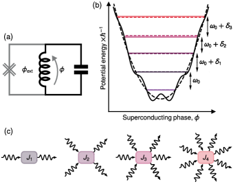
(a)

(b)

(c)

Figure 1: Principle of high-order photon processes. (a) Electrical circuit depicting a superconducting $LC$ oscillator (black) shunted by a generalized Josephson junction (grey) that only permits Cooper-pair tunneling in pairs. The circuit is threaded by an external flux denoted $\phi_{\text{ext}}$. (b) Potential and energy levels (solid lines) of this nonlinear oscillator [Eq. (1) with parameters in Tab. 1] and its linear equivalent (dashed lines) as a function of the superconducting phase difference at $\phi_{\mathrm{ext}}=\pi$. Crucially, the adjacent transition frequency shift $\delta_{n}$ from the bare frequency $\omega_{0}$ alternates in sign when ascending the ladder. (c) Photon process diagrams for the first four interaction orders and corresponding interaction energies $J_{n}$.

In the field of microwave quantum optics with superconducting circuits [8, 9, 10], the nonlinearity of the Josephson junction is employed to mediate interactions between photons. These photons are typically stored in an $LC$ circuit [11] of angular frequency $\Omega=1/\sqrt{LC}$ ($L$ and $C$ are the circuit inductance and capacitance, respectively). Superconductivity endows these circuits with low photon loss, and quality factors exceeding one million are routinely observed [12, 13, 14]. When such a circuit is shunted by a Josephson junction, interactions between photons appear (Fig. 1). The Hamiltonian takes the form

$$\hat{\mathcal{H}}_{\text{ideal}} =\hbar\Omega\hat{a}^{\dagger}\hat{a}-\mathcal{E}_{J}\cos(\hat{\phi}-\phi_{\text{ext}})$$

$$\hat{\phi} =\eta(\hat{a}+\hat{a}^{\dagger})\;,$$ (1)

where $\hbar$ is the reduced Planck constant and $\hat{a}$ is the photon annihilation operator. The interaction energy stems from the Josephson cosine potential with Josephson energy $\mathcal{E}_{J}$, and $\hat{\phi}$ is the phase drop across the junction with $\eta$ its zero-point fluctuations. The loop formed by the oscillator inductance and the junction is threaded by external magnetic flux denoted $\phi_{\text{ext}}$. Expanding the cosine into its Taylor series reveals the various interaction processes. For example, the $\left[\eta(\hat{a}+\hat{a}^{\dagger})\right]^{4}$ term yields a two-photon interaction term $\hat{a}^{{\dagger}^{2}}\hat{a}^{2}$ corresponding to the Kerr effect. A celebrated success of microwave quantum optics was the first realization of a Kerr interaction that exceeded the photon loss rate, demonstrating the collapse of a coherent state into multi-component Schrödinger cat states [15]. In this letter, we address the problem of inducing higher-order processes of the form $\hat{a}^{{\dagger}^{n}}\hat{a}^{n}$ where $n=3$, $4$, and beyond.

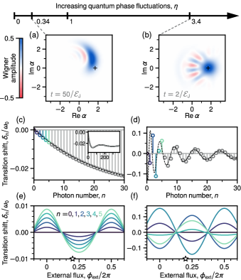
(a)

(b)

(c)

(d)

(e)

(f)

Figure 2: Signatures of higher-order photon processes. (a)–(b) Simulated Wigner quasiprobability distribution representing the initial time evolution of the coherent state $|\alpha\rangle$ with $\alpha=1.7$ for small and large quantum phase fluctuations. This value of $\alpha$ was chosen to match $\eta/2$ for $\eta=3.4$ (see text). As quantum phase fluctuations increase, the evolution remarkably transitions from diffusive to nondiffusive. Simulated transition frequency shifts $\delta_{n}=\omega_{n}-\omega_{0}$, where $\omega_{n}$ is the transition frequency between energy levels $n$ and $n+1$, are represented versus photon number at the starred external flux value (c)–(d), and versus external flux (e)–(f). We observe the transition from an ordered to an alternating arrangement that asymptotically approaches a Bessel function (dashed lines). Simulations correspond to numerical diagonalization and time propagation of Eq. (1) with parameters in Tab. 1.

The relative strength of multi-photon processes is governed by the dimensionless quantity $\eta$. It can be expressed as $\eta=\sqrt{\pi Z/R_{Q}}$, where $Z=\sqrt{L/C}$ is the $LC$ circuit impedance, and $R_{Q}\approx$6.4\text{\,}\mathrm{k\SIUnitSymbolOhm}$$ is the superconducting resistance quantum [16]. The $n$-photon process $\hat{a}^{{\dagger}^{n}}\hat{a}^{n}$ has a strength that scales as $\left(\eta^{n}/n!\right)^{2}$, and therefore, its activation for large $n$ requires entering the regime $\eta>1$, or equivalently $Z\gg R_{Q}$. However, fabricating an $LC$ oscillator with a characteristic impedance exceeding the superconducting resistance quantum is challenging, although progress is being made with the development of superinductances [17, 18, 19, 20]. Recently, $\eta\approx 1$ was achieved in a planar coil resonator, and emissions of $k$-photon bunches ($k=1\text{ to }6$) were observed by activating the process $\hat{a}^{k}+\hat{a}^{{\dagger}^{k}}$ with a voltage-biased junction [21].

Another route towards large phase fluctuations is to replace the Josephson junction, that allows Cooper-pair tunneling, by a dipole that only allows pairs of Cooper pairs to tunnel [Fig. LABEL:sub@fig:reduced_circuit]. In the basis of tunneled Cooper-pair number $N$, the tunneling operator is transformed as $\frac{1}{2}\sum_{N}{\left(\ket{N}\bra{N+1}+\ket{N+1}\bra{N}\right)}\rightarrow\frac{1}{2}\sum_{N}{\left(\ket{N}\bra{N+2}+\ket{N+2}\bra{N}\right)}$. Equivalently, in the conjugate phase representation $\varphi$, $\cos\hat{\varphi}\rightarrow\cos 2\hat{\varphi}$ [22, 23]. Denoting $\hat{\phi}=2\times\hat{\varphi}$, we see that phase fluctuations are effectively doubled: $\eta=2\times\sqrt{\pi Z/R_{Q}}$ [24]. In the extreme regime of $\eta>1$, we further require that $\mathcal{E}_{J}\ll\hbar\Omega$ [Fig. LABEL:sub@fig:potential], so that the Josephson cosine potential primarily induces $n$-photon interaction processes $\hat{a}^{{\dagger}^{n}}\hat{a}^{n}$ [Fig. LABEL:sub@fig:sketch].

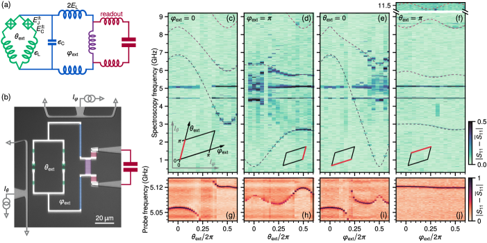
(a)

(b)

(c)

(d)

(e)

(f)

(g)

(h)

(i)

(j)

Figure 3: Experimental implementation. (a) Electrical circuit for the KITE (green) shunted by a superinductance (blue) and coupled through a shared inductance (purple) to an $LC$ oscillator used for dispersive readout. The two small junctions have slightly different Josephson energies $E_{J}^{\pm}=(1\pm\varepsilon)E_{J}$ and charging energies $E_{C}^{\pm}=E_{C}/(1\pm\varepsilon)$, with $\varepsilon\ll 1$, due to junction fabrication variation. (b) Optical micrograph of the physical device, with false color indicating the constituent Josephson junctions. Aluminum and niobium electrodes appear in white and grey, respectively. (c)–(f) Two-tone reflection spectroscopy (background subtracted) of the four lowest transitions from the ground state along the four edges of the primitive cell in the two-dimensional external flux landscape (inset diagrams), and (g)–(j) accompanying readout spectroscopy. Theoretical transition frequencies (dashed lines) are obtained from numerical diagonalization of the three-mode circuit model with six fitted Hamiltonian parameters. The dominance of two-Cooper-pair tunneling along the $\theta_{\mathrm{ext}}=\pi$ edge strikingly suppresses the residual flux dispersion of the first four transition frequencies.

In this experiment, we implement a superconducting $LC$ oscillator shunted by a two-Cooper-pair tunnel element. We place ourselves in the unexplored regime where the tunneling energy is smaller than the oscillator transition energies, and the zero-point phase fluctuations exceed one: $\mathcal{E}_{J}/\hbar\Omega=0.28$ and $\eta=3.4$. We measure the first four transition energies of our device, and find that unlike a Kerr resonator, they do not follow a monotonic trend. Instead, we observe an alternation of the sign of the oscillator frequency shift for each added photon. From this spectroscopic signature, we extract two-, three-, and four-photon interaction processes of amplitudes greater than $70\text{\,}\mathrm{MHz}$, that alternate in sign, and far exceed the transition linewidths of $200\text{\,}\mathrm{kHz}$. The realization of these unprecedentedly high-order photon processes opens avenues in microwave quantum optics, such as multi-photon quantum logic [4], the study of many-body photon states [6], or the processing of protected qubits [25].

We proceed to the analysis of the ideal Hamiltonian in Eq. (1) in the unexplored regime $\mathcal{E}_{J}\ll\hbar\Omega$ and $\eta>1$ (Fig. 1), and for simplicity, we set $\phi_{\text{ext}}=0$. Note that the cosine in Eq. (1) may be decomposed as $\cos\left[\eta(\hat{a}+\hat{a}^{\dagger})\right]=\frac{1}{2}\left(\hat{D}_{\eta}+\hat{D}_{-\eta}\right)$, where $\hat{D}_{\eta}=\exp\left[i\eta(\hat{a}+\hat{a}^{\dagger})\right]$ is the displacement evolution operator. Remarkably, this evolution operator that usually results from the integration of a linear Hamiltonian $\propto\hat{a}+\hat{a}^{\dagger}$ over time enters the Hamiltonian directly. As a consequence, even at short times, a quantum state evolving under this Hamiltonian in Eq. (1) will be displaced across phase-space by $\pm\eta$. The effect is particularly striking when initializing the system in a coherent state of amplitude $\alpha=\eta/2$ [25], so that $\ket{\pm\alpha}$, that are distant by $2\alpha$ is phase-space, are directly coupled through $\cos\left[\eta(\hat{a}+\hat{a}^{\dagger})\right]$ [Fig. LABEL:sub@fig:displacement_wigner]. This is qualitatively different from the familiar diffusive-like evolutions resulting from low-order photon interactions [15] [Fig. LABEL:sub@fig:kerr_wigner].

We now express $\hat{\mathcal{H}}_{\text{ideal}}$ in Eq. (1) in terms of $n$-photon interaction processes [Fig. LABEL:sub@fig:sketch]. We start by expanding the cosine into a normal ordered Taylor expansion. Then, by virtue of the rotating wave approximation (RWA), we neglect non-particle number conserving terms. We arrive at [26] :

$$\hat{\mathcal{H}}_{\text{ideal}}\approx\hbar\omega_{0}\hat{a}^{\dagger}\hat{a}+\sum_{n\geq 2}J_{n}\hat{a}^{{\dagger}^{n}}\hat{a}^{n}\;,$$ (2)

where the $n$-photon interaction energy takes the form $J_{n}=-\mathcal{E}_{J}e^{-{\eta^{2}}/2}(-1)^{n}\left({\eta^{n}}/n!\right)^{2}$, and the renormalized frequency is $\omega_{0}=\Omega+J_{1}/\hbar$. Note that $J_{n}/J_{n-1}=-(\eta/n)^{2}$, and hence the interaction strength is maximal for the integer order closest to $\eta$. The eigenenergies of Eq. (2) are $E_{n}=n\hbar\omega_{0}+\sum_{k=2}^{n}\frac{n!}{(n-k)!}J_{k}$, and the experimentally accessible quantities are the transition frequencies $\omega_{n}=(E_{n+1}-E_{n})/\hbar$. We introduce the transition frequency shift in the presence of $n$ photons as $\delta_{n}=\omega_{n}-\omega_{0}$ [Fig. LABEL:sub@fig:potential] and we find :

$$\delta_{n}=\sum_{k=2}^{n+1}k\frac{n!}{(n+1-k)!}J_{k}/\hbar\;.$$ (3)

In the familiar situation of the Kerr oscillator where $\eta\ll 1$, $J_{2}\approx-\mathcal{E}_{J}\eta^{4}/4$ is half the Kerr shift per photon and $J_{n\geq 3}$ can be neglected. Hence $\omega_{n}\approx\omega_{0}+2nJ_{2}/\hbar$ and the transition frequency monotonically shifts for each added photon [Figs. LABEL:sub@fig:kerr_photons and LABEL:sub@fig:kerr_flux]. This is in stark contrast with the regime of extreme phase fluctuations explored in this work where the transition frequency shift may alternate in sign for each added photon [Figs. LABEL:sub@fig:displacement_photons and LABEL:sub@fig:displacement_flux]. This resembles the oscillatory nonlinearity predicted in a resonator containing a phase-slip element [27].

Our circuit implementation of $\hat{\mathcal{H}}_{\text{ideal}}$ in Eq. (1) is depicted in Figs. LABEL:sub@fig:circuit_kite and LABEL:sub@fig:device. It consists of a high impedance $LC$ oscillator. The inductance, which we aim to maximize, is formed by a chain of $90$ Josephson junctions, resulting in an inductive energy $E_{L}/h=$0.53\text{\,}\mathrm{GHz}$$. The capacitance, which we aim to minimize, originates from the capacitance between the two wires linking the oscillator to the tunneling element, resulting in charging energy $\epsilon_{C}/h=$5.65\text{\,}\mathrm{GHz}$$. Tunneling occurs through a so-called Kinetic Interference coTunneling Element (KITE) [28, 24]. It consists of two parallel arms that form a loop threaded by an external flux $\theta_{\text{ext}}$. Each arm contains a small junction of Josephson energy $E_{J}^{\pm}=E_{J}(1\pm\epsilon)$ and charging energy $E_{C}^{\pm}=E_{C}/(1\pm\epsilon)$, with $E_{J}/h=$3.92\text{\,}\mathrm{GHz}$$, $E_{C}/h=$6.23\text{\,}\mathrm{GHz}$$ and fabrication uncertainty results in a small asymmetry factor $\epsilon=0.032$. Each small junction is placed in series with $6$ large junctions of a total inductive energy $\epsilon_{L}/h=$6.73\text{\,}\mathrm{GHz}$$. This non-vanishing series inductance induces the tunneling of pairs of Cooper-pairs. Finally, this circuit is inductively coupled to a resonator for readout [29].

The circuit parameters quoted above are extracted by fitting a three-mode circuit model [26] (discarding the readout mode) to two-tone spectroscopy data at various flux biases $(\theta_{\text{ext}},\varphi_{\text{ext}})$ [Figs. LABEL:sub@fig:twotone_theta_zero–LABEL:sub@fig:twotone_varphi_half]. This three-mode Hamiltonian is $2\pi$ periodic in $(\theta_{\text{ext}},\varphi_{\text{ext}})$ and its spectrum possesses inversion symmetry about $(\theta_{\text{ext}},\varphi_{\text{ext}})=(0,0)$, $(0,\pi)$, $(\pi,0)$, and $(\pi,\pi)$ [30]. Therefore, these four points are the vertices of a plaquette that constitutes the primitive cell of the circuit spectrum as a function of external flux. We acquire the circuit spectrum along the edges of this plaquette [diagrams in Figs. LABEL:sub@fig:twotone_theta_zero–LABEL:sub@fig:twotone_varphi_half]. At each bias point, we start by acquiring the reflection spectrum of the readout resonator [Figs. LABEL:sub@fig:readout_theta_zero–LABEL:sub@fig:readout_varphi_half]. We then set the readout tone on resonance, and sweep a probe tone over a broad spectral range [Figs. LABEL:sub@fig:twotone_theta_zero–LABEL:sub@fig:twotone_varphi_half]. When the probe hits a circuit transition from the ground state to the $n$-th excited state, the reflected readout signal is affected. We identify several transitions that are captured by a three-mode circuit model [26] (dashed lines). The feature near $4.4\text{\,}\mathrm{GHz}$ corresponds to a parasitic mode visible in electromagnetic simulations, and the one near $5.1\text{\,}\mathrm{GHz}$ corresponds to the readout resonator. Other non-captured features could arise from multi-photon transitions to higher excited states or junction array modes. The circuit parameters we extract from this fit are summarized in Tab. 1.

$E_{J}/h$	$E_{C}/h$	$E_{L}/h$	$\epsilon_{L}/h$	$\epsilon_{C}/h$	$\varepsilon$
3.92	6.23	0.53	6.73	5.65	0.032
$\Omega/2\pi$	$\mathcal{E}_{J}/h$	$\delta E_{J}/h$	$\eta$
2.86	0.79	0.27	3.40

Table 1: Extracted model parameters. The first line of parameters are found by fitting the spectral lines in Fig. LABEL:sub@fig:twotone_theta_zero–LABEL:sub@fig:twotone_varphi_half to the three-mode circuit Hamiltonian of Fig. LABEL:sub@fig:circuit_kite in the absence of the readout mode [26]. The second line of parameters are found by fitting the measured transition frequencies at $\theta_{\text{ext}}=\pi$ [Fig. LABEL:sub@fig:interlacing] to the effective one-mode Hamiltonian in Eq. (Spectral signature of high-order photon processes mediated by Cooper-pair pairing). All energy scales are given in gigahertz.

Importantly—at sufficiently low frequencies (here below about $20\text{\,}\mathrm{GHz}$)—our circuit is well described by a single-mode Hamiltonian that emulates the one in Eq. (1) [26]. Discarding the readout mode and the two KITE self-resonant high-frequency modes, we focus on the $LC$ oscillator of inductive energy $E_{L}$ and charging energy $\epsilon_{C}$. This oscillator is shunted by a KITE that renormalizes its frequency $\Omega$ and provides nonlinearity. In the regime $\epsilon_{L}\gg E_{J}$, the potential energy of one arm of the KITE traversed by a phase drop of $\varphi$ takes the form $U^{\pm}(\varphi)\approx-E^{\pm}_{J}\cos\varphi+\frac{{E_{J}^{\pm}}^{2}}{4\epsilon_{L}}\cos 2\varphi$ and higher harmonics have been neglected [26]. Biasing the circuit at $\theta_{\text{ext}}=\pi$, Cooper-pair tunneling across both arms interferes destructively, while cotunneling interferes constructively. Indeed, the potential energy of the KITE is $U^{+}(\varphi)+U^{-}(\varphi+\pi)\approx-\delta E_{J}\cos\varphi+\mathcal{E}_{J}\cos 2\varphi$, with $\delta E_{J}=2\epsilon E_{J}$ and $\mathcal{E}_{J}\approx E_{J}^{2}/2\epsilon_{L}$. Conveniently, $\mathcal{E}_{J}$ can be made smaller than the oscillator frequency $\Omega$ by adequately choosing $E_{J}$ and $\epsilon_{L}$. In summary, this yields an effective Hamiltonian for our circuit at $\theta_{\text{ext}}=\pi$ of the form [26]:

$$\hat{\mathcal{H}}_{\text{circuit}} =\hbar\Omega\hat{a}^{\dagger}\hat{a}+\mathcal{E}_{J}\cos[2(\hat{\varphi}-\varphi_{\text{ext}})]$$

$$\qquad\qquad-\delta E_{J}\cos(\hat{\varphi}-\varphi_{\text{ext}})\;,$$ (4)

where $\varphi_{\text{ext}}$ is the flux threading the loop formed by the KITE and the oscillator inductance. Note that $\hat{\mathcal{H}}_{\text{circuit}}$ corresponds to $\hat{\mathcal{H}}_{\text{ideal}}$ up to the perturbative term in $\delta E_{J}$, with the correspondence $\hat{\phi}=2\hat{\varphi}$ and $\phi_{\text{ext}}=2\varphi_{\text{ext}}+\pi$. Additionally, the $J_{n}$ obtained from Eq. (Spectral signature of high-order photon processes mediated by Cooper-pair pairing) depend on external flux and contain an added contribution from the term in $\delta E_{J}$.

We extract the parameters of the one-mode Hamiltonian in Eq. (Spectral signature of high-order photon processes mediated by Cooper-pair pairing) by fitting this model to the measured transition energies at $\theta_{\text{ext}}=\pi$ [Fig. LABEL:sub@fig:interlacing]. The resulting parameters are displayed in Tab. 1. Two notable features are visible in the data. First, these transition frequencies vary in a $\pm$500\text{\,}\mathrm{MHz}$$ window—a $\pm$17\text{\,}\mathrm{\char 37\relax}$$ fraction of the central frequency $\Omega/2\pi=$2.86\text{\,}\mathrm{GHz}$$. This confirms that the flux dependent tunneling amplitude is a perturbation to the $LC$ oscillator frequency, i.e. $\mathcal{E}_{J},\delta E_{J}<\hbar\Omega$. In particular, we find $\mathcal{E}_{J}/h=$0.79\text{\,}\mathrm{GHz}$$ and the perturbation $\delta E_{J}/h=$0.27\text{\,}\mathrm{GHz}$$. Second, the transition frequencies $\omega_{n}$ between levels $n$ and $n+1$ are not ordered in $n$. Instead, they interlace as a function of $\varphi_{\text{ext}}$, indicating that we have entered the regime of large phase fluctuations. For example, at $\varphi_{\text{ext}}=0.2$, $\omega_{0}>\omega_{1}$, $\omega_{1}<\omega_{2}$, and $\omega_{2}>\omega_{3}$ [Fig. LABEL:sub@fig:Kn]. From this measured spectrum, we compute the $n$-photon interaction strengths $J_{n}$ for $n=2$, $3$, and $4$ [Fig. LABEL:sub@fig:Jn] by inverting Eq. (3) . Notably, we find that $|J_{2}|\approx|J_{3}|$, which is consistent with the extracted $\eta=3.4$.

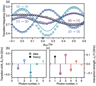
(a)

(b)

(c)

Figure 4: Spectral interlacing. (a) Adjacent transition frequencies obtained from two-tone measurements (open circles) and numerical diagonalization of the one-mode Hamiltonian (solid curves) along $\theta_{\mathrm{ext}}=\pi$. (b) Transition frequency shifts $\delta_{n}$ and (c) interaction strengths $J_{n}$ extracted from measurements (open circles) and analytic expressions depending on the fitted circuit parameters (fitted circles) at the starred external flux value. The transition frequency shifts alternate in sign while remaining much smaller than the transition frequency itself, directly corresponding to similarly-sized Hamiltonian coefficients for four-wave, six-wave, and eight-wave mixing.

In conclusion, this experiment explores a new regime of nonlinear microwave quantum optics where interactions between photons are so strong that second-, third-, and fourth-order processes are of comparable amplitude and largely exceed the photon decay rate. We access this regime with photons stored in a high impedance $LC$ oscillator that is shunted by a two-Cooper-pair tunneling element, effectively boosting phase fluctuations. Two technical challenges must be met: the tunneling energy $\mathcal{E}_{J}$ must be weaker than the oscillator energy $\hbar\Omega$, and the phase fluctuations $\eta$ across the tunneling element must exceed one. We measure the first four transition frequencies of our circuit, and observe their interlacing versus flux. From these spectra, we extract $\mathcal{E}_{J}/\hbar\Omega=0.28$ and $\eta=3.4$. The observation of high-order photon processes could be extended in multiple directions. One is the study of the quantum dynamics and scattered radiation correlations of this system under the action of drives and dissipation [27]. Moreover, coupling our two-Cooper-pair tunneling element to an array of resonators could induce high-order interactions between multiple modes, useful for the study of many-body photon states [5, 6]. Finally, applications are envisioned to process quantum information that is encoded non-locally over the phase space of an oscillator [25].

Acknowledgments: W.C.S acknowledges fruitful discussions with Agustin Di Paolo. The devices were fabricated within the consortium Salle Blanche Paris Centre. We thank Jean-Loup Smirr and the Collège de France for providing nano-fabrication facilities. This work was supported by the QuantERA grant QuCOS, by ANR 19-QUAN-0006-04. This project has received funding from the European Research Council (ERC) under the European Union’s Horizon 2020 research and innovation program (grant agreement no. 851740). This work has been funded by the French grants ANR-22-PETQ-0003 and ANR-22-PETQ-0006 under the “France 2030 Plan.”

Supplementary Material

S1 Device fabrication

This section details the fabrication process we follow to produce the sample of this experiment.

Wafer preparation:

The circuit is fabricated on a $430\text{\,}\mathrm{\SIUnitSymbolMicro m}$-thick wafer of 0001-oriented, double-side epi-polished Sapphire C. The sapphire wafer is initially cleaned through a stripping process in a reactive ion etching (RIE) machine, after which it is loaded into a sputtering system. After one night of pumping, we initiate an argon milling cleaning step, followed by the sputtering of $120\text{\,}\mathrm{nm}$ of niobium. Subsequently, we apply a protective layer of poly(methyl methacrylate) (PMMA A6), dice the wafer and clean the small chips in solvents. This is followed by a $2\text{\,}\mathrm{min}$ oxygen-stripping process and approximately $30\text{\,}\mathrm{s}$ of exposure to sulphur hexafluoride (SF6) in order to remove the oxide layer formed on the niobium during the stripping process.

Circuit patterning:

We spin optical resist (S1805) and pattern the large features (control lines and readout resonator capacitor pads) using a laser writer. After development (MF319), we rinse in de-ionized water for $1\text{\,}\mathrm{min}$, and etch the sample in SF6 with a $20\text{\,}\mathrm{s}$ over-etch. Finally, the sample is cleaned for $10\text{\,}\mathrm{min}$ in acetone at $50\text{\,}\mathrm{\SIUnitSymbolCelsius}$.

Junction patterning:

Next, we apply a bilayer of methacrylic acid/methyl methacrylate [MMA (8.5) MAA EL10] and poly(methyl methacrylate) (PMMA A6). The entire circuit (KITE, inductive shunt, and readout resonator) is patterned in a single e-beam lithography step. The development takes place in a 3:1 isopropyl alcohol (IPA)/water solution at $6\text{\,}\mathrm{\SIUnitSymbolCelsius}$ for $90\text{\,}\mathrm{s}$, followed by $10\text{\,}\mathrm{s}$ in IPA. The undercut regions of the bilayer are cleaned by oxygen-stripping for $30\text{\,}\mathrm{s}$.

Junction deposition:

The chip is then loaded in an e-beam evaporator. We start with a thorough argon ion milling for $2\text{\,}\mathrm{min}$ at $\pm 30\text{\,}\mathrm{\SIUnitSymbolDegree}$ angles. We then evaporate $35\text{\,}\mathrm{nm}$ and $100\text{\,}\mathrm{nm}$ of aluminum, at $\pm 30\text{\,}\mathrm{\SIUnitSymbolDegree}$ angles, separated by an oxidation step in $200\text{\,}\mathrm{mbar}$ of pure oxygen for $10\text{\,}\mathrm{min}$.

Junction characteristics:

The Josephson junctions are all fabricated from Al/AlOx/Al in a single evaporation step, utilizing the Dolan bridge method. The e-beam base dose is set to $283\text{\,}\mathrm{\SIUnitSymbolMicro C}\text{\,}{\mathrm{cm}}^{-2}$, with an acceleration voltage of $20\text{\,}\mathrm{kV}$ and a lens aperture of $7.5\text{\,}\mathrm{\SIUnitSymbolMicro m}$. Three types of junctions are fabricated. (i) Two small junctions are located in the KITE, with an area of $0.076\text{\,}{\mathrm{\SIUnitSymbolMicro m}}^{2}$. They are patterned with a dose factor of $0.9$ and an undercut dose of $0.2$, resulting in an inductance per junction of $42\text{\,}\mathrm{nH}$. (ii) A total of $12$ large array junctions are found within the KITE loop, along with a further $90$ unshared shunting array junctions. These junctions have an area of $0.62\text{\,}{\mathrm{\SIUnitSymbolMicro m}}^{2}$, and are patterned with a dose factor of $0.9$ and an undercut dose of $0.1$, resulting in an inductance per junction of $4\text{\,}\mathrm{nH}$. (iii) There are $29$ larger array junctions that constitute the readout resonator inductance, $19$ of which are shared. These junctions have an area of $3\text{\,}{\mathrm{\SIUnitSymbolMicro m}}^{2}$, and are patterned with a dose factor of $0.8$ and an undercut dose of $0.1$, resulting in an inductance per junction of $0.7\text{\,}\mathrm{nH}$.

Sample mounting:

The chip was subsequently glued with PMMA onto a PCB, wire-bonded and mounted into a sample holder. The device was then thermally anchored to the base plate of a Bluefors dilution refrigerator, surrounded by three concentric cans for magnetic and infrared shielding (outer: cryoperm, middle: aluminum, inner: copper). An optical micrograph of the circuit and SEM images of some junctions are shown in Fig. S5.

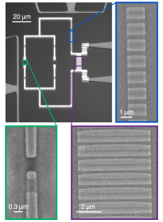
Figure S5: Optical micrograph of the device and scanning electron microscope images of the three Josephson junction types from a nominally identical sample. (Green) one of the two small KITE junctions. (Blue) $14$ of the array junctions that form both the internal KITE inductance and the inductive shunt. (Purple) $12$ of the array junctions that form the shared inductance between the circuit and the readout resonator, as well as the self-inductance of the readout. All junctions are fabricated in one step using Dolan bridges.

S2 Mathematical derivations

In this section we derive the expression of the $n$-photon interaction strength $J_{n}$ that enters Eq. (2), as well as Eq. (3) that relates $J_{n}$ to the transition frequency shift $\delta_{n}$.

We start from Hamiltonian (1) with $\phi_{\text{ext}}=0$ for simplicity. Note that the cosine may be decomposed as $\cos\left[\eta(\hat{a}+\hat{a}^{\dagger})\right]=\frac{1}{2}\left(\exp\left[i\eta(\hat{a}+\hat{a}^{\dagger})\right]+\exp\left[-i\eta(\hat{a}+\hat{a}^{\dagger})\right]\right)$. Since the commutator $[\hat{a}^{\dagger},\hat{a}]$ commutes with both $\hat{a}$ and $\hat{a}^{\dagger}$, we may use Glauber’s formula as follows $\exp\left[i\eta(\hat{a}+\hat{a}^{\dagger})\right]=e^{-\eta^{2}/2}e^{i\eta\hat{a}^{\dagger}}e^{i\eta\hat{a}}$. We then expand each exponential into its Taylor series. Since we place ourselves in the regime $\hbar\Omega\gg\mathcal{E}_{J}$, we perform the rotating wave approximation (RWA) by neglecting terms that do not conserve particle number, yielding

$$\cos\hat{\phi}\biggr{\rvert}_{\text{RWA}}=e^{-\eta^{2}/2}\sum_{n=0}^{+\infty}(-1)^{n}\left(\frac{\eta^{n}}{n!}\right)^{2}\hat{a}^{{\dagger}^{n}}\hat{a}^{n}\;.$$

Inserting this last equation in Eq. (1) yields Hamiltonian (2) with :

$$J_{n}=-\mathcal{E}_{J}e^{-\eta^{2}/2}(-1)^{n}\left({\eta^{n}}/{n!}\right)^{2}\;.$$

We now turn to the derivation of Eq. (3). The eigenvectors of Hamiltonian (2) are Fock states $\ket{n}$ where $n$ is an integer. Using the formula: for $n\geq 0$, $\hat{a}^{\dagger}\ket{n}=\sqrt{n+1}\ket{n+1}$ and for $n\geq 1$, $\hat{a}\ket{n}=\sqrt{n}\ket{n-1}$ and $\hat{a}\ket{0}=0$, their associated eigenvalue $E_{n}$ take the form

$$E_{n}=n\hbar\omega_{0}+\sum_{k=2}^{n}\frac{n!}{(n-k)!}J_{k}\;.$$

We define the transition frequency $\omega_{n}=(E_{n+1}-E_{n})/\hbar$, and $\delta_{n}=\omega_{n}-\omega_{0}$. Note that

$$E_{n+1}=(n+1)\hbar\omega_{0}+(n+1)!J_{n+1}+\sum_{k=2}^{n}\frac{(n+1)!}{(n+1-k)!}J_{k}\;,$$

so that

$$\hbar\delta_{n} =(n+1)!J_{n+1}+\sum_{k=2}^{n}\left(\frac{(n+1)!}{(n+1-k)!}-\frac{n!}{(n-k)!}\right)J_{k}$$

$$=(n+1)!J_{n+1}+n!\sum_{k=2}^{n}k\frac{n!}{(n+1-k)!}J_{k}$$

$$=\sum_{k=2}^{n+1}k\frac{n!}{(n+1-k)!}J_{k}\;.$$

S3 Harmonics from single arm KITE

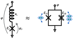
Figure S6: Electrical circuit diagrams depicting the emergence of Josephson harmonics when a linear inductance is connected in series with a Josephson junction without its self-capacitance (left). Imposing Kirchhoff’s current law on the central node yields an effective potential containing both one- and two-Cooper-pair tunneling terms (right).

In this section we demonstrate that a Josephson junction in series with a small inductance generates Josephson harmonics [32]. We carry out this simple derivation at zero frequency where capacitors may be disregarded. We consider the circuit depicted in Fig. S6, in the regime where the inductive energy $\epsilon_{L}$ largely exceeds the Josephson energy $E_{J}$. We denote $\nu=E_{J}/\epsilon_{L}$ (here $\nu\ll 1$), $\varphi$ the phase drop across the entire circuit, and $\varphi_{J}$ the phase drop across the junction alone. The potential energy $U$ of this circuit is the sum of the inductive energy $U_{L}=\frac{1}{2}\epsilon_{L}(\varphi-\varphi_{J})^{2}$ and the Josephson energy $U_{J}=-E_{J}\cos\varphi_{J}$. This yields $U=\epsilon_{L}\left[\frac{1}{2}(\varphi-\varphi_{J})^{2}-\nu\cos\varphi_{J}\right]$. Also, $\varphi_{J}$ is tied to $\varphi$ though Kirchhoff’s current law $E_{J}\sin\varphi_{J}=\epsilon_{L}(\varphi-\varphi_{J})$. This equation may be recast as $\varphi_{J}=\varphi-\nu\sin\varphi_{J}$, and to first order in $\nu$, simplified to $\varphi_{J}=\varphi-\nu\sin\varphi+\mathcal{O}(\nu^{2})$. Injecting this expression in the inductive energy yields $U_{L}=\frac{1}{2}\epsilon_{L}\left[\nu^{2}\sin^{2}\varphi+\mathcal{O}(\nu^{3})\right]$ and $U_{J}=-\epsilon_{L}\left[\nu\cos\varphi+\nu^{2}\sin^{2}\varphi+\mathcal{O}(\nu^{3})\right]$. Summing these two energies results in $U=-\epsilon_{L}\left[\nu\cos\varphi+\frac{1}{2}\nu^{2}\sin^{2}\varphi+\mathcal{O}(\nu^{3})\right]$. Finally, disregarding an irrelevant constant, we recover

$$U(\varphi)=-E_{J}\cos\varphi+\frac{1}{2}\frac{E_{J}^{2}}{2\epsilon_{L}}\cos 2\varphi+\epsilon_{L}\mathcal{O}\left[(E_{J}/\epsilon_{L})^{3}\right]\;.$$ (S5)

The first term in this expression is the usual Josephson energy that allows Cooper-pair tunneling. The second term is the second Josephson harmonic, and is responsible for the tunneling of pairs of Cooper pairs (Fig. S6). The remaining perturbative term encompasses higher order harmonics.

S4 Model reduction

S4.1 Outline of analysis

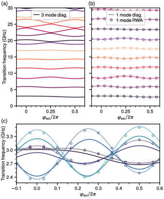
Figure S8: Comparison of models of the device. (a–b) Transition frequencies from the ground state obtained from numerical diagonalization of the three-mode Hamiltonian in Eq. (S6) and the one-mode Hamiltonian in Eq. (S10) with parameters in the first row of Tab. 1, in addition to analytic results from RWA with the same parameters. Note the difference between these parameters and those obtained from a Hamiltonian fit (first and second rows of Tab. S2, respectively). (c) Adjacent transition frequencies emphasizing the differences between the three models.

In this section, we describe the mathematical procedure for reducing the three-mode Hamiltonian of an $LC$ oscillator shunted by a KITE to an effective one-mode Hamiltonian. The procedure that we use is not mathematically rigorous, yet it provides a reduced model that agrees both qualitatively and, to a lesser extent, quantitatively with the full circuit model (see Fig. S8). Improving the agreement and establishing a firm mathematical foundation will be the subject of future work [33]. We neglect the readout resonator and consider the circuit in Fig. S7. To realize the Hamiltonian in Eq. (Spectral signature of high-order photon processes mediated by Cooper-pair pairing) at $\theta_{\mathrm{ext}}=\pi$, we first place ourselves in the parameter regime $E_{L}\ll\epsilon_{C}\sim E_{C}$, which guarantees large phase fluctuations in the oscillator. Second, we require $E_{J}\lesssim\epsilon_{L}\ll E_{J}/\varepsilon$ to lower the two-Cooper-pair tunneling energy below the bare Josephson energy $E_{J}$ while keeping single-Cooper-pair tunneling a perturbation. Finally, making the oscillator frequency the largest energy scale in the effective Hamiltonian (but still much smaller than the junction plasma frequency), we arrive at the parameter regime $E_{L}\ll\epsilon_{C}\sim E_{C},E_{J}\lesssim\epsilon_{L}$ and $\varepsilon\ll 1$.

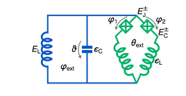
Figure S7: Electrical circuit diagram for the KITE (green) shunted by a superinductance and a capacitance (blue). As in the main text, we have $E_{J}^{\pm}=(1\pm\varepsilon)E_{J}$ and $E_{C}^{\pm}=E_{C}/(1\pm\varepsilon)$.

Our analysis is organized as follows. We first write down the exact Hamiltonian for the circuit in Fig. S7 and move to a basis where the kinetic energy is diagonal and the modes are weakly coupled. Then, we derive the low-frequency component of the Hamiltonian evaluated at the equilibrium positions of the high-frequency modes. Finally, we derive the ground state energy of the high-frequency component and combine the results into an effective single-mode low-energy Hamiltonian.

S4.2 Three-mode Hamiltonian and basis transformation

We start with the circuit Hamiltonian [30]

$$\hat{H} =\frac{2E_{C}}{1-\varepsilon^{2}}(\hat{N}_{\Sigma}^{2}+\hat{N}_{\Delta}^{2}-2\varepsilon\hat{N}_{\Sigma}\hat{N}_{\Delta})+4\epsilon_{C}\hat{M}^{2}+\frac{1}{2}E_{L}\hat{\vartheta}^{2}$$

$$+\epsilon_{L}\left(\hat{\vartheta}-\hat{\varphi}_{\Sigma}-\varphi_{\mathrm{ext}}-\tfrac{1}{2}\theta_{\mathrm{ext}}\right)^{2}+\epsilon_{L}\left(\hat{\varphi}_{\Delta}-\tfrac{1}{2}\theta_{\mathrm{ext}}\right)^{2}$$

$$-2E_{J}\cos\hat{\varphi}_{\Sigma}\cos\hat{\varphi}_{\Delta}+2\varepsilon E_{J}\sin\hat{\varphi}_{\Sigma}\sin\hat{\varphi}_{\Delta}\;,$$ (S6)

where we have introduced symmetric and antisymmetric variables $\hat{\varphi}_{\Sigma}=\frac{1}{2}(\hat{\varphi}_{1}+\hat{\varphi}_{2})$ and $\hat{\varphi}_{\Delta}=\frac{1}{2}(\hat{\varphi}_{1}-\hat{\varphi}_{2})$. Note that $\hat{\bm{N}}=\begin{pmatrix}\hat{N}_{\Sigma}&\hat{N}_{\Delta}&\hat{M}\end{pmatrix}^{\mathrm{T}}$ are the conjugate Cooper-pair numbers to $\hat{\bm{\phi}}=\begin{pmatrix}\hat{\varphi}_{\Sigma}&\hat{\varphi}_{\Delta}&\hat{\vartheta}\end{pmatrix}^{\mathrm{T}}$. Unfortunately, model reduction using the Born-Oppenheimer approximation would be inefficient in this basis due to the strong coupling between $\hat{\vartheta}$ and $\hat{\varphi}_{\Sigma}$ arising from the large value of $\epsilon_{L}$ relative to the other energy scales.

To remedy this, we move to a basis where the dominant terms in the Hamiltonian are diagonal. The Hamiltonian in Eq. (S6) may be decomposed into two parts: a linear Hamiltonian that accounts for the energy of the capacitances and internal KITE inductance (proportional to $E_{C}$, $\epsilon_{C}$, and $\epsilon_{L}$), and a nonlinear potential (proportional to $E_{L}$ and $E_{J}$). In our parameter regime, we can regard the latter as a perturbation and proceed by diagonalizing the former, which has the form

$$\lim_{\begin{subarray}{c}E_{J}\rightarrow 0\\ E_{L}\rightarrow 0\end{subarray}}\hat{H}=4\hat{\bm{N}}^{\mathrm{T}}\mathbb{E}_{C}\hat{\bm{N}}+\tfrac{1}{2}\hat{\bm{\phi}}^{\mathrm{T}}\mathbb{E}_{L}\hat{\bm{\phi}}$$

$$\mathbb{E}_{C}=\epsilon_{C}\begin{pmatrix}z&-\varepsilon z&0\\ -\varepsilon z&z&0\\ 0&0&1\end{pmatrix}\qquad\mathbb{E}_{L}=2\epsilon_{L}\begin{pmatrix}1&0&-1\\ 0&1&0\\ -1&0&1\end{pmatrix}$$

upon a gauge transformation to shift $\hat{\varphi}_{\Sigma}\rightarrow\hat{\varphi}_{\Sigma}-\varphi_{\mathrm{ext}}-\frac{1}{2}\theta_{\mathrm{ext}}$ and $\hat{\varphi}_{\Delta}\rightarrow\hat{\varphi}_{\Delta}+\frac{1}{2}\theta_{\mathrm{ext}}$. We have also defined $z=\frac{E_{C}}{2\epsilon_{C}(1-\varepsilon^{2})}=\frac{E_{C}}{2\epsilon_{C}}+\mathcal{O}(\varepsilon^{2})$ to parameterize the degree of capacitive loading, which diverges in the limit of vanishing junction capacitance. This linear Hamiltonian can be diagonalized with the transformation

$$\hat{\bm{\phi}}=\Lambda\hat{\bm{\varphi}}$$

$$\Lambda=\begin{pmatrix}1&(z-1)\varepsilon&-z\\ 0&1&z(1+z)\varepsilon\\ 1&-\varepsilon&1\end{pmatrix}+\mathcal{O}(\varepsilon^{2})\;,$$

which has the effect of shuttling the coupling from terms of order $\epsilon_{L}$ to terms of smaller order $E_{J}$ and $E_{L}$. We denote the transformed superconducting phases $\hat{\bm{\varphi}}=\begin{pmatrix}\hat{\varphi}&\hat{\theta}&\hat{\zeta}\end{pmatrix}^{\mathrm{T}}$. Note that in the limit of vanishing junction asymmetry and capacitance, $z$ diverges and $\hat{\vartheta}\rightarrow\hat{\varphi}$. Recalling that the charging and inductive energy matrices transform according to $\mathbb{E}_{C}\rightarrow\Lambda^{-1}\mathbb{E}_{C}(\Lambda^{\mathrm{T}})^{-1}$ and $\mathbb{E}_{L}\rightarrow\Lambda^{\mathrm{T}}\mathbb{E}_{L}\Lambda$, we arrive at the Hamiltonian

$$\hat{H} =\frac{4\epsilon_{C}}{1+z^{-1}}\hat{N}_{\varphi}^{2}+2E_{C}\hat{N}_{\theta}^{2}+\frac{4\epsilon_{C}}{1+z}\hat{N}_{\zeta}^{2}$$

$$+\epsilon_{L}\hat{\theta}^{2}+\epsilon_{L}(1+z)^{2}\hat{\zeta}^{2}$$

$$+\frac{1}{2}E_{L}\left(\hat{\varphi}+\hat{\zeta}-\varepsilon\hat{\theta}+\varphi_{\mathrm{ext}}+\tfrac{1}{2}\theta_{\mathrm{ext}}\right)^{2}$$

$$-2E_{J}\cos\left[\hat{\varphi}-z\hat{\zeta}+(z-1)\varepsilon\hat{\theta}\right]$$

$$\qquad\times\cos\left[\hat{\theta}+z(1+z)\varepsilon\hat{\zeta}+\tfrac{1}{2}\theta_{\mathrm{ext}}\right]$$

$$+2\varepsilon E_{J}\sin\left(\hat{\varphi}-z\hat{\zeta}\right)\sin\left(\hat{\theta}+\tfrac{1}{2}\theta_{\mathrm{ext}}\right)+\epsilon_{L}\,\mathcal{O}(\varepsilon^{2})\;,$$ (S7)

where we have introduced the transformed conjugate Cooper-pair numbers $\hat{N}_{\varphi}$, $\hat{N}_{\theta}$, and $\hat{N}_{\zeta}$; and shifted $\hat{\varphi}\rightarrow\hat{\varphi}+\varphi_{\mathrm{ext}}+\frac{1}{2}\theta_{\mathrm{ext}}$. Note that the charging energy of the $\hat{\varphi}$ mode approaches $\epsilon_{C}$ when the junction capacitance vanishes. On the other hand, when the shunting capacitance and junction asymmetry vanish, the Josephson potential terms in Eq. (S7) are identical to those in Eq. (S6).

	$\Omega/2\pi$	$\mathcal{E}_{J}/h$	$\delta E_{J}/h$	$\eta$
Analytic	2.93	1.14	0.25	3.31
One-mode fit	2.86	0.79	0.27	3.40

Table S2: Comparison of the effective circuit parameters. The top row is obtained from fitting the data to the one-mode Hamiltonian, while the second row is obtained from analytic model reduction with physical circuit parameters found by fitting to the three-mode Hamiltonian.

S4.3 Born-Oppenheimer approximation

In our parameter regime, $\epsilon_{L}$ is the dominant energy scale. Therefore, the Hamiltonian in Eq. (S7) describes two high-frequency modes $\hat{\theta}$ and $\hat{\zeta}$, and one low-frequency mode $\hat{\varphi}$, which are all perturbatively coupled through the terms proportional to $E_{J}$ and $E_{L}$. Our goal is to derive an effective Hamiltonian for the low-frequency $\hat{\varphi}$ mode. A method that is well suited for this purpose is the Born-Oppenheimer approximation, where one sets $\hat{\varphi}$ to a classical parameter $\varphi$ in Eq. (S7) and removes the kinetic term proportional to $\hat{N}_{\varphi}^{2}$, yielding the Hamiltonian $\hat{H}_{\theta\zeta}$. One then needs to calculate the ground state energy $E_{0}(\varphi)$ of $\hat{H}_{\theta\zeta}$. The Born-Oppenheimer approximation states that the effective potential of the $\hat{\varphi}$ mode is well captured by $E_{0}(\hat{\varphi})$. However, an analytic expression for $E_{0}(\varphi)$ is unknown. Instead, we seek a low-order expansion of Eq. (S7) in order to analytically compute an approximate expression for $E_{0}(\varphi)$.

We recall that we are placed in the parameter regime where $E_{L}\ll E_{J}\lesssim\epsilon_{L}$. In the following, we will assume $E_{J}/\epsilon_{L}=\mathcal{O}(\lambda)$ and $E_{L}/E_{J}=\mathcal{O}(\lambda)$, where $\lambda$ is a small parameter. In the semiclassical limit of vanishing quantum fluctuations of $\hat{\theta}$ and $\hat{\zeta}$, the effective potential of $\hat{\varphi}$ coincides with the full potential $\hat{U}$ from Eq. (S7) evaluated at the equilibrium values $\hat{\theta}_{0}$ and $\hat{\zeta}_{0}$. The equilibrium values themselves are found by solving $\frac{\partial\hat{U}}{\partial\hat{\theta}}\big{|}_{\hat{\theta}_{0},\hat{\zeta}_{0}}=0$ and $\frac{\partial\hat{U}}{\partial\hat{\zeta}}\big{|}_{\hat{\theta}_{0},\hat{\zeta}_{0}}=0$. Retaining only the lowest-order terms in $\lambda$ and $\varepsilon$, we find

$$\hat{\theta}_{0} =-\frac{E_{J}}{\epsilon_{L}}\left[\sin\tfrac{1}{2}\theta_{\mathrm{ext}}\cos\hat{\varphi}+\mathcal{O}(\lambda,\varepsilon)\right]$$

$$\hat{\zeta}_{0} =\frac{E_{J}z}{\epsilon_{L}(1+z)^{2}}\left[\cos\tfrac{1}{2}\theta_{\mathrm{ext}}\sin\hat{\varphi}+\mathcal{O}(\lambda,\varepsilon)\right]\;.$$ (S8)

The low-frequency Hamiltonian can then be calculated—in the semiclassical limit of vanishing fluctuations of the phases $\hat{\theta}$ and $\hat{\zeta}$—to be

$$\hat{H}_{\varphi} =\frac{4\epsilon_{C}}{1+z^{-1}}\hat{N}_{\varphi}^{2}+\hat{U}\Big{|}_{\hat{\theta}_{0},\hat{\zeta}_{0}}$$

$$=\frac{2E_{C}}{1+z}\hat{N}_{\varphi}^{2}+\frac{1}{2}E_{L}\left(\hat{\varphi}+\varphi_{\mathrm{ext}}+\tfrac{1}{2}\theta_{\mathrm{ext}}\right)^{2}$$

$$-\frac{E_{J}^{2}}{2\epsilon_{L}}\left[\sin^{2}\tfrac{1}{2}\theta_{\mathrm{ext}}-\frac{z^{2}}{(1+z)^{2}}\cos^{2}\tfrac{1}{2}\theta_{\mathrm{ext}}\right]\cos 2\hat{\varphi}$$

$$-2E_{J}\cos\tfrac{1}{2}\theta_{\mathrm{ext}}\cos\hat{\varphi}+2\varepsilon E_{J}\sin\tfrac{1}{2}\theta_{\mathrm{ext}}\sin\hat{\varphi}$$

$$+\lambda E_{J}\,\mathcal{O}(\lambda,\varepsilon)+E_{C}\,\mathcal{O}(\varepsilon^{2})\;.$$ (S9)

Finally, shifting $\hat{\varphi}\rightarrow\hat{\varphi}-\varphi_{\mathrm{ext}}-\frac{1}{2}\theta_{\mathrm{ext}}$ and setting $\theta_{\mathrm{ext}}=\pi$ yields the single-mode model referenced in the main text,

$$\hat{H}_{\varphi}\Big{|}_{\pi} =\frac{4\epsilon_{C}}{1+z^{-1}}\hat{N}_{\varphi}^{2}+\frac{1}{2}E_{L}\hat{\varphi}^{2}+\frac{E_{J}^{2}}{2\epsilon_{L}}\cos\left[2(\hat{\varphi}-\varphi_{\mathrm{ext}})\right]$$

$$-2\varepsilon E_{J}\cos(\hat{\varphi}-\varphi_{\mathrm{ext}})$$

$$+\lambda E_{J}\,\mathcal{O}(\lambda,\varepsilon)+E_{C}\,\mathcal{O}(\varepsilon^{2})$$ (S10)

after neglecting constant terms. We see that the shunting capacitance renormalizes the charging energy, while the inductive energy is completely unchanged. The first, second, and third terms in the potential represent the contributions of the inductive shunt, two-Cooper-pair tunneling, and asymmetric dc-SQUID, respectively.

The Hamiltonian in Eq. (S10) is the main result of this section, and it explains both the approximate values of the effective parameters $\Omega$, $\mathcal{E}_{J}$, $\delta E_{J}$, and $\eta$ of the low-energy Hamiltonian as well as the functional form. Overall, we sought a lowest-order result in the the parameters $\varepsilon$ and $\lambda$, and completely neglected fluctuations of the high frequency modes. The parameters achieved in the experiment are not especially deep in this parameter regime—for instance $E_{J}/\epsilon_{L}=0.58$ and the fluctuations of $\hat{\theta}$ are of order $\left(\frac{E_{C}}{2\epsilon_{L}}\right)^{1/4}=0.82$ (similarly for $\hat{\zeta}$)—making the effective parameters in Eq. (S10) differ slightly from those found using a fit (see Tab. S2). Improved accuracy is likely possible using higher order corrections in $\lambda$ and including fluctuations.

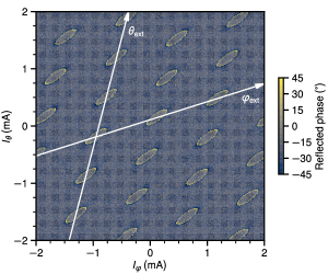
Figure S9: Reflected readout resonator phase as a function of dc current in both loop and KITE flux bias lines (respectively the top and left current sources in Fig. 3b) at probe frequency $5.055\,32\text{\,}\mathrm{GHz}$. The phase response is periodic in two directions, which we identify with white arrows to be the independent external fluxes $\varphi_{\mathrm{ext}}$ and $\theta_{\mathrm{ext}}$.

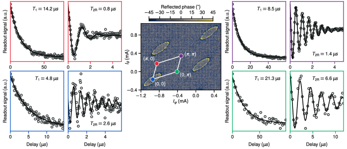
Figure S10: Qubit coherence times measured at the four distinct flux sweet spots, as indicated by colored circles in the central panel, which is a zoom of the wide external flux map in Fig. S9. The sweet spots are labeled by their coordinates $(\theta_{\mathrm{ext}},\varphi_{\mathrm{ext}})$, and the white lines connecting them correspond to the axes used for the spectroscopy data in Fig. 3.

S5 External flux dependence and coherence times

Due to their layout, our physical flux bias lines (see Fig. 3b) inevitably couple to both circuit external fluxes $\varphi_{\mathrm{ext}}$ and $\theta_{\mathrm{ext}}$. For initial characterization, we probe the readout resonator at the single frequency $5.055\,32\text{\,}\mathrm{GHz}$ and measure the reflected phase as a function of both bias currents. As the resulting pattern is 2D-periodic with many flux quanta visible, we can easily find the affine transformation that maps bias currents to $\varphi_{\mathrm{ext}}$ and $\theta_{\mathrm{ext}}$, as shown in Fig. S9. Additionally, we observe external flux drifts on the order of $1$–$2\text{\,}\mathrm{\char 37\relax}$ of a flux quantum on daily timescales, which we calibrate regularly using the procedure described in Ref. 30.

In addition to the spectroscopy data shown in the main text, we acquire coherence data of the lowest frequency transition—the qubit—at the four external flux sweet spots, as shown in Fig. S10. As visible in Fig. 3, the qubit frequency varies by an order of magnitude from $636\text{\,}\mathrm{MHz}$ to $6.882\text{\,}\mathrm{GHz}$ as the external flux point is stepped from $(\theta_{\mathrm{ext}},\varphi_{\mathrm{ext}})=(0,\pi)$ to $(\pi,\pi)$ to $(\pi,0)$ to $(0,0)$; in other words, counter-clockwise around the plaquette in Fig. S10 starting at the green point. As the qubit frequency increases, the observed relaxation times decrease from $21.3\text{\,}\mathrm{\SIUnitSymbolMicro s}$ to $4.8\text{\,}\mathrm{\SIUnitSymbolMicro s}$, indicating a roughly constant quality factor loss channel such as dielectric loss. The coherence times measured with a Ramsey sequence range from $0.8$–$6.6\text{\,}\mathrm{\SIUnitSymbolMicro s}$ and improve by about a factor of two using a single echo pulse (not shown). The dephasing is likely due to a combination of second-order flux noise, phase-slips in the array junctions, and photon shot noise in the readout resonator.

References

Chang et al. [2014]D. E. Chang, V. Vuletić, and M. D. Lukin, Quantum
nonlinear optics — photon by photon, Nature Photonics 8, 685 (2014).
Liang et al. [2018]Q.-Y. Liang, A. V. Venkatramani, S. H. Cantu, T. L. Nicholson, M. J. Gullans, A. V. Gorshkov, J. D. Thompson, C. Chin,
M. D. Lukin, and V. Vuletić, Observation of three-photon bound
states in a quantum nonlinear medium, Science 359, 783 (2018).
Drori et al. [2023]L. Drori, B. C. Das,
T. D. Zohar, G. Winer, E. Poem, A. Poddubny, and O. Firstenberg, Quantum vortices of strongly interacting photons, Science 381, 193 (2023).
Adhikari et al. [2013]P. Adhikari, M. Hafezi, and J. M. Taylor, Nonlinear optics quantum computing
with circuit QED, Phys. Rev. Lett. 110, 060503 (2013).
Greentree et al. [2006]A. D. Greentree, C. Tahan,
J. H. Cole, and L. C. L. Hollenberg, Quantum phase transitions of light, Nature Physics 2, 856–861 (2006).
Ma et al. [2019]R. Ma, B. Saxberg,
C. Owens, N. Leung, Y. Lu, J. Simon, and D. I. Schuster, A
dissipatively stabilized Mott insulator of photons, Nature 566, 51–57 (2019).
Carusotto et al. [2020]I. Carusotto, A. A. Houck, A. J. Kollár,
P. Roushan, D. I. Schuster, and J. Simon, Photonic materials in circuit quantum electrodynamics, Nature Physics 16, 268–279 (2020).
Wallraff et al. [2004]A. Wallraff, D. I. Schuster, A. Blais,
L. Frunzio, R.-S. Huang, J. Majer, S. Kumar, S. M. Girvin, and R. J. Schoelkopf, Strong
coupling of a single photon to a superconducting qubit using circuit quantum
electrodynamics, Nature 431, 162 (2004).
Hofheinz et al. [2009]M. Hofheinz, H. Wang,
M. Ansmann, R. C. Bialczak, E. Lucero, M. Neeley, A. D. O'Connell, D. Sank, J. Wenner, J. M. Martinis, and A. N. Cleland, Synthesizing arbitrary
quantum states in a superconducting resonator, Nature 459, 546 (2009).
Lang et al. [2013]C. Lang, C. Eichler,
L. Steffen, J. M. Fink, M. J. Woolley, A. Blais, and A. Wallraff, Correlations, indistinguishability and entanglement in
Hong–Ou–Mandel experiments at microwave
frequencies, Nature Physics 9, 345 (2013).
Devoret [1997]M. H. Devoret, Quantum fluctuations in
electrical circuits, in Quantum Fluctuations (Les Houches Session LXIII), edited by S. Reynaud, E. Giacobino, and J. Zinn-Justin (North-Holland, 1997) pp. 351–386.
Place et al. [2021]A. P. M. Place, L. V. H. Rodgers, P. Mundada, B. M. Smitham, M. Fitzpatrick, Z. Leng,
A. Premkumar, J. Bryon, A. Vrajitoarea, S. Sussman, G. Cheng, T. Madhavan, H. K. Babla, X. H. Le, Y. Gang, B. Jäck, A. Gyenis, N. Yao, R. J. Cava, N. P. de Leon, and A. A. Houck, New material platform for
superconducting transmon qubits with coherence times exceeding 0.3
milliseconds, Nature
Communications 12, 10.1038/s41467-021-22030-5
(2021).
Ganjam et al. [2023]S. Ganjam, Y. Wang,
Y. Lu, A. Banerjee, C. U. Lei, L. Krayzman, K. Kisslinger, C. Zhou, R. Li, Y. Jia, M. Liu, L. Frunzio, and R. J. Schoelkopf, Surpassing millisecond coherence times in on-chip superconducting
quantum memories by optimizing materials, processes, and circuit design
(2023), arXiv:2308.15539 .
Kono et al. [2023]S. Kono, J. Pan, M. Chegnizadeh, X. Wang, A. Youssefi, M. Scigliuzzo, and T. J. Kippenberg, Mechanically induced correlated errors on superconducting qubits with
relaxation times exceeding 0.4 milliseconds (2023), arXiv:2305.02591
.
Kirchmair et al. [2013]G. Kirchmair, B. Vlastakis, Z. Leghtas,
S. E. Nigg, H. Paik, E. Ginossar, M. Mirrahimi, L. Frunzio, S. M. Girvin, and R. J. Schoelkopf, Observation of quantum state collapse and revival due to the single-photon
Kerr effect, Nature 495, 205 (2013).
Manucharyan et al. [2009]V. E. Manucharyan, J. Koch,
L. I. Glazman, and M. H. Devoret, Fluxonium: Single Cooper-pair
circuit free of charge offsets, Science 326, 113 (2009).
Peruzzo et al. [2020]M. Peruzzo, A. Trioni,
F. Hassani, M. Zemlicka, and J. M. Fink, Surpassing the resistance quantum with a geometric
superinductor, Phys. Rev. Applied 14, 044055 (2020).
Pechenezhskiy et al. [2020]I. V. Pechenezhskiy, R. A. Mencia, L. B. Nguyen,
Y.-H. Lin, and V. E. Manucharyan, The superconducting quasicharge qubit, Nature 585, 368 (2020).
Rieger et al. [2022]D. Rieger, S. Günzler,
M. Spiecker, P. Paluch, P. Winkel, L. Hahn, J. K. Hohmann, A. Bacher, W. Wernsdorfer, and I. M. Pop, Granular aluminium
nanojunction fluxonium qubit, Nature Materials 22, 194 (2022).
Ménard et al. [2022]G. C. Ménard, A. Peugeot,
C. Padurariu, C. Rolland, B. Kubala, Y. Mukharsky, Z. Iftikhar, C. Altimiras, P. Roche, H. le Sueur, P. Joyez, D. Vion, D. Esteve, J. Ankerhold, and F. Portier, Emission of photon multiplets by a
dc-biased superconducting circuit, Phys. Rev. X 12, 021006 (2022).
Douçot and Vidal [2002]B. Douçot and J. Vidal, Pairing of Cooper pairs
in a fully frustrated Josephson-junction chain, Phys. Rev. Lett. 88, 227005 (2002).
Ioffe and Feigel’man [2002]L. B. Ioffe and M. V. Feigel’man, Possible realization
of an ideal quantum computer in Josephson junction array, Phys. Rev. B 66, 224503 (2002).
Smith et al. [2020]W. C. Smith, A. Kou, X. Xiao, U. Vool, and M. H. Devoret, Superconducting circuit protected by two-Cooper-pair
tunneling, npj Quantum Inf. 6, 8 (2020).
Cohen et al. [2017]J. Cohen, W. C. Smith,
M. H. Devoret, and M. Mirrahimi, Degeneracy-preserving quantum nondemolition
measurement of parity-type observables for cat qubits, Phys. Rev. Lett. 119, 060503 (2017).
[26]Supplementary material.
Hriscu and Nazarov [2011]A. M. Hriscu and Y. V. Nazarov, Model of a proposed
superconducting phase slip oscillator: A method for obtaining few-photon
nonlinearities, Phys. Rev. Lett. 106, 077004 (2011).
Bell et al. [2014]M. T. Bell, J. Paramanandam,
L. B. Ioffe, and M. E. Gershenson, Protected Josephson rhombus
chains, Phys. Rev. Lett. 112, 167001 (2014).
Smith et al. [2016]W. C. Smith, A. Kou, U. Vool, I. M. Pop, L. Frunzio, R. J. Schoelkopf, and M. H. Devoret, Quantization
of inductively shunted superconducting circuits, Phys. Rev. B 94, 144507 (2016).
Smith et al. [2022]W. C. Smith, M. Villiers,
A. Marquet, J. Palomo, M. R. Delbecq, T. Kontos, P. Campagne-Ibarcq, B. Douçot, and Z. Leghtas, Magnifying quantum phase fluctuations with
Cooper-pair pairing, Phys. Rev. X 12, 021002 (2022).
Note [1]Notice that is experimentally inaccessible since it
corresponds to the shift between the measured transition frequency and the resonance in the absence of the tunneling
element.
Willsch et al. [2023]D. Willsch, D. Rieger,
P. Winkel, M. Willsch, C. Dickel, J. Krause, Y. Ando, R. Lescanne, Z. Leghtas,
N. T. Bronn, P. Deb, O. Lanes, Z. K. Minev, B. Dennig, S. Geisert, S. Günzler, S. Ihssen, P. Paluch, T. Reisinger, R. Hanna, J. H. Bae, P. Schüffelgen, D. Grützmacher, L. Buimaga-Iarinca, C. Morari, W. Wernsdorfer,
D. P. DiVincenzo,
K. Michielsen, G. Catelani, and I. M. Pop, Observation of Josephson harmonics in tunnel junctions
(2023), arXiv:2302.09192 .