Exact finite-time correlation functions for multi-terminal setups:
Connecting theoretical frameworks for quantum transport and thermodynamics

Abstract

Transport in open quantum systems can be explored through various theoretical frameworks, including the quantum master equation, scattering matrix, and Heisenberg equation of motion. The choice of framework depends on factors such as the presence of interactions, the coupling strength between the system and environment, and whether the focus is on steady-state or transient regimes. Existing literature treats these frameworks independently, lacking a unified perspective. Our work addresses this gap by clarifying the role and status of these approaches using a minimal single-level quantum dot model in a two-terminal setup under voltage and temperature biases. We derive analytical expressions for particle and energy currents and their fluctuations in both steady-state and transient regimes. Exact results from the Heisenberg equation are shown to align with scattering matrix and master equation approaches within their respective validity regimes. Crucially, we establish a protocol for the weak-coupling limit, bridging the applicability of master equations at weak-coupling with Heisenberg or scattering matrix approaches at arbitrary coupling strength.

I Introduction

Recent advancements in quantum technologies have revitalized interest in the field of open quantum systems, captivating diverse physics communities, each with distinct methodologies and goals. A focal point within this domain is quantum transport [1, 2, 3], where the emphasis lies on assessing out-of-equilibrium average currents and corresponding correlations for particles, charges and energy. These quantities hold significance in thermodynamics from both theoretical [4, 5, 6] and experimental perspectives [7, 8, 9, 10, 11], playing a crucial role in addressing fundamental topics such as fluctuation-dissipation relations [12, 13] and thermodynamic uncertainty relations [14, 15, 16, 17], and practical ones such as quantum metrology [18, 19, 20].

Transport in open quantum systems can be explored through various theoretical frameworks, each relying on distinct central concepts and deriving average currents and current correlations from different perspectives. Conventional quantum transport approaches, such as the Landauer-Büttiker theory [21, 22], Green’s functions and Keldysh formalism [23, 24, 25, 26], are centered around the number of particles in a reservoir without direct reference to the quantum state of the system. Conversely, the knowledge of the state of a quantum system is fundamentally important in the field of quantum information. The typical approach towards this problem is the quantum master equation [27, 28, 29, 30], focusing on the density operator describing the state of the system and incorporating environmental effects perturbatively under the assumption of weak system-bath coupling. Given that significant progress in quantum thermodynamics has been driven by quantum information [31], the master equation approach has naturally emerged as the primary choice for computations in this area.

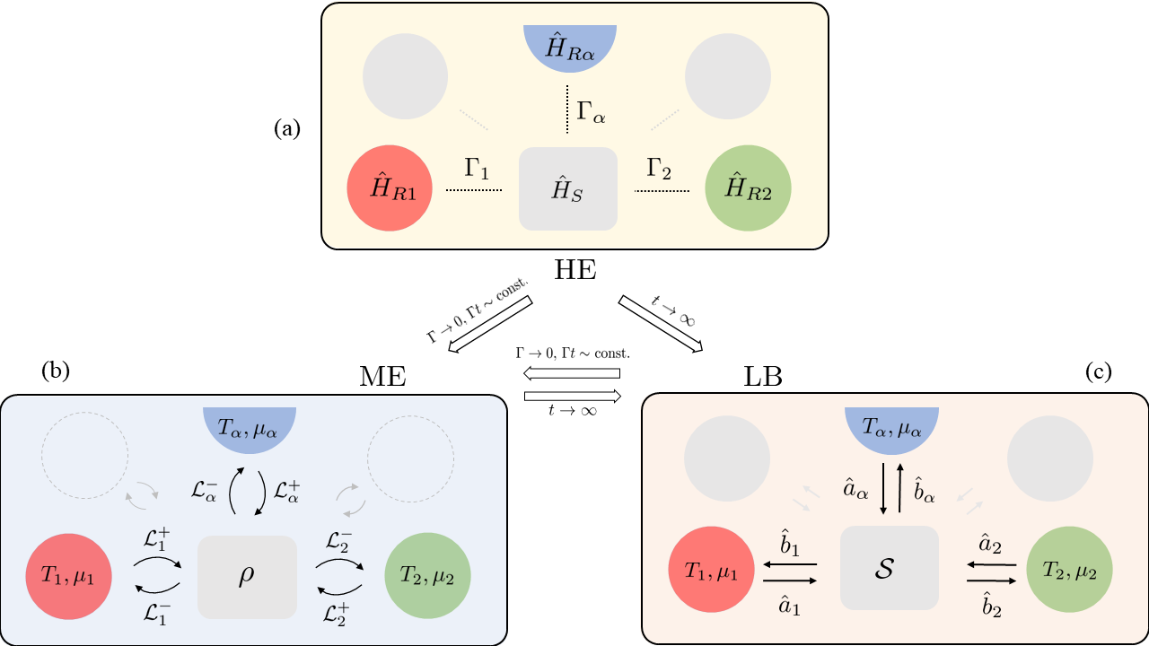
Figure 1: Schematic representation of the three approaches considered in this work: Heisenberg equation of motion (HE), Master equation (ME) and Landauer-Büttiker (LB). The details of these approaches to assess the dynamics of an open quantum system coupled to multiple reservoirs can be found in Sec. II. The thick arrows represent the limits necessary to move between the results of each approach.

Irrespective of the approach, existing literature predominantly explores steady-state observables due to the inherent complexity in deriving exact analytical finite-time solutions. For example, recent efforts have introduced techniques combining quantum stochastic Hamiltonians with Keldysh formalism [32, 33], however, at present, their complexity limits their applicability to the steady-state. Notably, exact results for current correlations are known only for a single resonant level with non-equilibrium Green’s functions approach [34]. Furthermore, in the master equation approach, currents and fluctuations are typically derived either in the steady state with full counting statistics (see, for example, Ref. [35]), or under a stochastic framework [36, 37, 38, 32, 39], while the Landauer-Büttiker approach predominantly focuses on the zero-frequency component of currents correlations, limited to the steady state [40].

Despite shared motivations, the techniques employed in quantum transport and thermodynamics often differ, posing a challenge for researchers transitioning between these backgrounds. Bringing approaches from quantum transport and thermodynamics under the same umbrella is therefore a natural and timely pursuit. From a practical perspective, this means that it should be possible to recover exactly the results from any approach by means of a unifying framework. As discussed in [41, 42, 43], this is not a trivial task, as each framework has its own domain of validity and unique assumptions. Therefore, it is typically challenging to determine how the results of one framework and its corresponding implications can be understood in the context of another. Specifically, establishing a connection between approaches at the level of current correlations is an open problem.

In this work, we focus on three main approaches to open quantum systems and quantum transport: the Heisenberg equation of motion (HE), the quantum master equation (ME), and the Landauer-Büttiker approach (LB). In the ME framework, we further generalize the full counting statistics (FCS) approach, to account for multiple terminals, multiple times, and non-instantaneous jumps, as compared to existing literature [35, 44, 45]. Our work pursues two primary objectives: (1) establishing connections between different frameworks for assessing open quantum system dynamics, developing a protocol for the weak-coupling limit from exact solutions, as depicted in Fig. 1; and (2) providing explicit and complete analytical results for auto- and cross-correlation functions of current considering a minimal single-level quantum dot model, using the Heisenberg equation of motion and the master equation, as summarized in Table 1. This paradigmatic model serves as a benchmark, facilitating comparisons across approaches and validating the protocol for deriving weak-coupling and stationary limits. Importantly, our results go beyond the simple example discussed and can serve as building blocks to investigate higher-dimensional and many-body open quantum systems. The techniques introduced in this work can be applied to understand the operation of quantum devices for any couplings and for finite-times, for example, to investigate the build up of quantum correlations beyond simple setups [46].

The article is organized as follows. We start in Sec. II by delineating a general model of an open quantum system alongside the HE, ME, and LB frameworks within the context of quantum transport. In Sec. II.2.1, we introduce a generalized full counting statistics (GFCS) approach for the calculation of current and current correlations accounting for multiple times, multiple terminals and extended to arbitrary quanta of particles, charges, or energies exchange between system and reservoirs. After providing a brief description of the single-level quantum dot model, we present exact analytical solutions for currents and their fluctuations using the HE approach in Sec. IV, followed by the corresponding solutions using the ME approach in Sec. V. We benchmark both approaches against the LB approach in the steady state. Finally, in Sec. VI, we present a weak-coupling procedure connecting observables calculated with the HE and LB frameworks with the results obtained from the ME. We conclude in Sec. VII, offering perspectives for further exploration.

II Model and frameworks for quantum transport

We consider a time-independent system of $D$ fermionic quantum dots coupled to $N$ reservoirs through tunneling interactions as depicted in Fig. 1 (a). The total Hamiltonian $\hat{H}$ is composed of the following terms,

$$\hat{H}=\hat{H}_{S}+\sum_{\alpha=1}^{N}\hat{H}_{R_{\alpha}}+\sum_{\alpha=1}^{N}\hat{H}_{SR_{\alpha}}.$$ (1)

$\hat{H}_{S}$ represents the system Hamiltonian with non-degenerate bare energies $\epsilon_{j}$,

$$\hat{H}_{S}=\sum_{j=1}^{D}\epsilon_{j}\hat{d}_{j}^{\dagger}\hat{d}_{j}\,,$$ (2)

with the fermionic creation and annihilation operators $\hat{d}_{j}^{\dagger},\hat{d}_{j}$, obeying the anti-commutation relations $\{d_{i},d_{j}^{\dagger}\}=\delta_{ij}$. The free fermionic Hamiltonian for each reservoir $\alpha$ is given by,

$$\hat{H}_{R_{\alpha}}=\sum_{k}\epsilon_{k\alpha}\hat{c}_{k\alpha}^{\dagger}\hat{c}_{k\alpha}\,,$$ (3)

where $\hat{c}_{k\alpha}^{\dagger}$ and $\hat{c}_{k\alpha}$ are the creation and annihilation operators for the $k$-th mode in reservoir $\alpha$, corresponding to energy $\epsilon_{k\alpha}$ and obeying the anti-commutation relations $\{c_{k\alpha},c^{\dagger}_{k^{\prime}\alpha^{\prime}}\}=\delta_{kk^{\prime}}\delta_{\alpha\alpha^{\prime}}$. Finally, the system-reservoir interaction Hamiltonian takes the form,

$$\hat{H}_{SR_{\alpha}}=\sum_{jk}t_{jk\alpha}^{*}\hat{c}_{k\alpha}^{\dagger}\hat{d}_{j}+t_{jk\alpha}\hat{d}^{\dagger}_{j}\hat{c}_{k\alpha}\,,$$ (4)

where $t_{jk\alpha}$ represents the tunneling amplitude between the $j$-th level and the $k$-th mode of reservoir $\alpha$. The total Hamiltonian $\hat{H}$ describes a family of resonant-level systems [47, 48, 49], and represents a paradigmatic model for investigating quantum transport. Let us remark that although for simplicity we have considered non-interacting dots, interactions within the system can be taken into account by considering the problem in a basis that diagonalizes $\hat{H}_{S}$ [49].

The main goal of this work is to explore the transient and steady-state transport properties of the open quantum system governed by the Hamiltonian $\hat{H}$ as defined in Eq. (1). Our investigation focuses on three distinct approaches. The first approach employs the Heisenberg equation of motion (HE), providing exact solutions for all times and system-environment coupling strengths. The second approach involves the quantum master equation (ME), which is applicable in the weak-coupling regime. The third approach follows the Landauer-Büttiker formalism (LB), utilizing the scattering matrix in the steady-state regime. For each approach, we outline the key assumptions and detail the computation of fundamental transport quantities. In particular we will focus on particle current $I_{\alpha}$, energy current $J_{\alpha}$, and current correlation function $S_{\alpha\alpha^{\prime}}$. We specifically concentrate on particle and energy currents within the reservoirs due to their importance in quantum thermodynamics and their utility in deriving other thermodynamically relevant quantities. For instance, the charge current ($I^{c}_{\alpha}$) can be expressed as $I^{c}_{\alpha}(t)=eI_{\alpha}(t)$, where $e$ represents the elementary charge. Similarly, the heat current ($J^{h}_{\alpha}$) can be written as $J^{h}_{\alpha}(t)=J_{\alpha}(t)+J_{c\alpha}(t)/2-\mu_{\alpha}I_{\alpha}(t)$, with $\mu_{\alpha}$ denoting the chemical potential at reservoir $\alpha$, and $J_{c\alpha}$ representing the energy current in the contact region between the system and reservoir $\alpha$. As highlighted in Refs. [50, 51], including the contact energy current in the heat current definition is crucial to uphold the second law of thermodynamics in the transient regime. In our investigation, we do not focus on this term, as we have verified its negligibility in both the stationary and weak-coupling regimes. Specifically, in Appendix F, we provide evidence for the single resonant level case, demonstrating that this term precisely vanishes in the steady-state and only contributes in second order to the coupling strength in the weak-coupling regime.

II.1 Heisenberg equation approach

In the Heisenberg equation (HE) picture, the evolution of the operators $\hat{d}_{j}$ and $\hat{c}_{k\alpha}$ of the system and reservoir $\alpha$ is given by the Heisenberg equations of motion (we assume $\hbar,k_{B}=1$),

$$\frac{d}{dt}\hat{d}_{j}=-i[\hat{H},\hat{d}_{j}]\,$$ (5)

$$\frac{d}{dt}\hat{c}_{k\alpha}=-i[\hat{H},\hat{c}_{k\alpha}]$$ (6)

where $\hat{H}$ is the total Hamiltonian of Eq. (1). In the solution to Eqs. (5) and (6), a crucial quantity arises, which we will further examine in the specific case of a single-level quantum dot system in Sec. IV. This quantity is represented by the bare tunneling rate $\Gamma_{j\alpha}(\epsilon)$, which describes the strength of the system-bath coupling between the energy level $j$ of the system and the reservoir $\alpha$,

$$\Gamma_{j\alpha}(\epsilon)=2\pi\sum_{k}|t_{jk\alpha}|^{2}\delta\left(\epsilon-\epsilon_{k\alpha}\right).$$ (7)

This function encapsulates the impact of the reservoirs on the system and generally depends on the energy. Further assumptions on the sum $\sum_{k}|t_{jk\alpha}|^{2}$ yield well-known profiles for this quantity, such as the Ohmic or Lorentzian shapes as functions of energy [52]. An important limit under consideration in this work is the wide-band limit (WBL), where the energy width of $\Gamma_{j\alpha}(\epsilon)$ is larger than all other energy scales of the system. The WBL assumes an energy-independent spectral density, expressed as [53, 54, 55],

$$\Gamma_{j\alpha}(\epsilon)\equiv\Gamma_{j\alpha}\,.$$ (8)

In essence, in the WBL, the tunneling probabilities of the particles become insensitive to the energy structure of the bath; the system cannot resolve it. In the specific case of a single-level quantum dot discussed subsequently, the WBL approximation enables the derivation of analytical results. In Fig. 1 (a), we indicate with $\Gamma_{\alpha}=\sum_{j}\Gamma_{j\alpha}$ the total tunneling rate associated with reservoir $\alpha$.

Using the solutions to the above Eqs. (5) and (6), observable quantities can be calculated for all times. Specifically, quantum transport observables, i.e., currents and current-correlation function can be defined using the time-dependent occupation number operator in a given reservoir $\alpha$,

$$\hat{N}_{\alpha}(t)=\sum_{k}\hat{c}_{k\alpha}^{\dagger}(t)\hat{c}_{k\alpha}(t),$$ (9)

the operators $\hat{c}_{k\alpha}^{\dagger}(t),\hat{c}_{k\alpha}(t)$ being solutions of Eq. (6) for the creation and annihilation operators. The average particle current, $I_{\alpha}^{\text{HE}}$, and energy current, $J_{\alpha}^{\text{HE}}$, in lead $\alpha$, are defined as,

$$I_{\alpha}^{\text{HE}}(t) = \frac{d}{dt}\langle\hat{N}_{\alpha}\rangle=-i\left\langle[\hat{H},\hat{N}_{\alpha}]\right\rangle\,,$$ (10)

$$J_{\alpha}^{\text{HE}}(t) = \frac{d}{dt}\langle\hat{H}_{R_{\alpha}}\rangle=-i\left\langle[\hat{H},\hat{H}_{R_{\alpha}}]\right\rangle\,,$$ (11)

where $\langle\ldots\rangle$ denotes the quantum statistical average. The solutions depend on initial conditions at time $t=t_{0}$,

$$\expectationvalue{\hat{c}_{k\alpha}^{\dagger}(t_{0})\hat{c}_{k^{\prime}\alpha^{\prime}}(t_{0})}=\delta_{k\alpha,k^{\prime}\alpha^{\prime}}f_{\alpha}(\epsilon_{k\alpha})\,,$$ (12)

$$\expectationvalue{\hat{d}^{\dagger}_{i}(t_{0})\hat{d}_{j}(t_{0})}=\delta_{ij}n_{j}\,.$$ (13)

The first condition assumes that the initial mean occupation of the $\alpha$ reservoir is set by the Fermi-Dirac distribution at temperature $T_{\alpha}$ and chemical potential $\mu_{\alpha}$,

$$f_{\alpha}(\epsilon)=\{e^{(\epsilon-\mu_{\alpha})/T_{\alpha}}+1\}^{-1}\,.$$ (14)

The second condition assumes that the initial occupation population of the $j$-th energy level is $n_{j}$, while initial coherences among different levels are assumed to be zero. Fluctuations of the particle current at the reservoir $\alpha$ at time $t$ are accessed through the operator $\Delta\hat{I}_{\alpha}(t)\coloneqq\hat{I}_{\alpha}(t)-\expectationvalue{\hat{I}_{\alpha}}$, from which the current correlation function depending on times $t,t^{\prime}$ and leads $\alpha,\alpha^{\prime}$ is defined,

$$S_{\alpha\alpha^{\prime}}^{\text{HE}}(t,t^{\prime}) = \expectationvalue{\Delta\hat{I}_{\alpha}(t)\Delta\hat{I}_{\alpha^{\prime}}(t^{\prime})}$$ (15)

$$= \expectationvalue{\hat{I}_{\alpha}(t)\hat{I}_{\alpha^{\prime}}(t^{\prime})}-I_{\alpha}^{\text{HE}}(t)I_{\alpha^{\prime}}^{\text{HE}}(t^{\prime})\,.$$

The case $\alpha=\alpha^{\prime}$ corresponds to the auto-correlation function, while $\alpha\neq\alpha^{\prime}$ gives the cross-correlations.

The HE approach exactly addresses the evolution of operators for both the quantum system and the reservoirs, stemming from the unitary evolution dictated by total Hamiltonian $\hat{H}$, giving solutions that are entirely quantum coherent. In the subsequent discussion (see Sec. IV), we use this framework to derive exact expressions for currents and correlations for a single-level quantum dot model.

II.2 Master equation approach

The master equation (ME) framework serves as a paradigmatic approach for analyzing the dynamics of quantum systems weakly coupled with one or multiple reservoirs. In contrast to the Heisenberg equation approach, it is crucial to highlight that the central quantity of interest within the master equation framework is the reduced density operator of the quantum system, denoted as $\rho$, which satisfies the non-unitary evolution equation [28],

$$\dot{\rho}=-i~{}\text{Tr}_{R}\left\{[\hat{H},\rho_{\text{tot}}]\right\}\,.$$ (16)

Here, $\hat{H}$ represents the total Hamiltonian from Eq. (1), and $\rho_{\text{tot}}$ is the total density operator describing the system and all reservoirs. In contrast, $\rho$ is the reduced density operator of the quantum system, obtained by tracing out the degrees of freedom of the reservoirs ($\text{Tr}_{R}\left\{\ldots\right\}$). Under the assumption of weak-coupling between the system and reservoirs, the evolution equation for $\rho$ is governed by the Liouvillian superoperator $\mathcal{L}$. This superoperator corresponds to a CPTP (Completely Positive and Trace Preserving) map in Lindblad form [56, 57, 28], encompassing the unitary evolution of the quantum system according to its Hamiltonian $\hat{H}_{S}$, along with a dissipative part. Unlike Eq. (16), it exclusively describes the evolution of the reduced density operator $\rho$ of the system. In terms of the creation and annihilation operators of the system, $d_{j}^{\dagger},\hat{d}_{j}$, it takes the form,

$$\dot{\rho}(t)=\,\mathcal{L}\rho(t)= -i[\hat{H}_{S},\rho(t)]$$ (17)

$$+\sum_{\alpha j}\left(\Gamma_{j\alpha}^{+}\mathcal{D}[\hat{d}_{j}^{\dagger}]\rho(t)+\Gamma_{j\alpha}^{-}\mathcal{D}[\hat{d}_{j}]\rho(t)\right).$$

It can also be derived using the Feynman-Vernon influence functional theory [58, 59, 60, 61], or using Green’s function formalism [43], by performing a perturbative expansion in the system-reservoir coupling. In the above equation, the in- and out-tunneling rates are the product of the bare tunneling rates introduced in Eq. (7) and the occupation probability of the reservoir $\alpha$ given by the Fermi-Dirac distribution evaluated at the energy level $\epsilon_{j}$ [28],

$$\Gamma_{j\alpha}^{+} = \Gamma_{j\alpha}(\epsilon_{j})f_{\alpha}(\epsilon_{j})$$ (18)

$$\Gamma_{j\alpha}^{-} = \Gamma_{j\alpha}(\epsilon_{j})\big{(}1-f_{\alpha}(\epsilon_{j})\big{)}\,.$$ (19)

The dissipators $\mathcal{D}[\hat{d}_{j}]$ and $\mathcal{D}[\hat{d}_{j}^{\dagger}]$ are superoperators acting on $\rho$ and are defined as $\mathcal{D}[X]\rho\coloneqq X\rho X^{\dagger}-1/2(X^{\dagger}X\rho+\rho X^{\dagger}X)$ with $X=d_{j},d_{j}^{\dagger}$. The first term, $X\rho X^{\dagger}$, corresponds to quantum jumps, while the last two terms ensure trace conservation of the density operator $\rho$ for $\mathcal{L}$ to be a valid CPTP map.

It is convenient, for the remaining part of the section, to single out the role of the quantum jumps, which will directly enter the definitions of the currents and current correlation functions, and rewrite the Liouvillian superoperator $\mathcal{L}$ of Eq. (17) in the following form,

$$\dot{\rho}(t)=\mathcal{L}\,\rho(t)=\left(\mathcal{L}_{0}+\sum_{j\alpha}(\mathcal{L}^{+}_{j\alpha}+\mathcal{L}^{-}_{\alpha j})\right)\rho(t).$$ (20)

Here, $\mathcal{L}_{0}$ represents the coherent non-unitary evolution of the reduced state of the system and can be expressed in terms of a non-hermitian commutator, $\left[A,B\right]_{\dagger}=AB-B^{\dagger}A^{\dagger}$,

$$\mathcal{L}_{0}\rho=-i\left[\hat{H}_{S}-\frac{i}{2}\sum_{j\alpha}(\Gamma_{j\alpha}^{-}\hat{d}_{j}^{\dagger}\hat{d}_{j}+\Gamma_{j\alpha}^{+}\hat{d}_{j}\hat{d}_{j}^{\dagger}),\rho\right]_{\dagger}.$$ (21)

The jump superoperator $\mathcal{L}^{+}_{j\alpha}$ ($\mathcal{L}^{-}_{j\alpha}$) captures the tunneling in (out) of particles from (to) reservoir $\alpha$ to (from) the energy level $\epsilon_{j}$ of the quantum system with corresponding rate $\Gamma_{j\alpha}^{+}$ ($\Gamma_{j\alpha}^{-}$),

$$\mathcal{L}^{+}_{j\alpha}\rho = \Gamma_{j\alpha}^{+}\,\hat{d}^{\dagger}_{j}\,\rho\,\hat{d}_{j}$$ (22)

$$\mathcal{L}^{-}_{j\alpha}\rho = \Gamma_{j\alpha}^{-}\,\hat{d}_{j}\,\rho\,\hat{d}^{\dagger}_{j}\,.$$ (23)

II.2.1 Generalized Full Counting Statistics (GFCS)

A convenient method for calculating currents and correlation functions by solving Eq. (20) is Full Counting Statistics (FCS). In the standard FCS approach, the emphasis is on the steady state [35], and quantum jumps are assumed to be instantaneous [39, 37]. Here, we develop a generalized approach to FCS that not only accommodates multiple terminals and times but also considers non-instantaneous jumps. To achieve this, we initially discretize Eq. (20) in terms of the net amount of particles, charges, or energy quanta exchanged between the reservoirs and the system. For this purpose, we introduce the $\vec{x}$-resolved state of the system, denoted as $\rho^{(\vec{x})}\left(t\right)$, which satisfies [30],

$$\dot{\rho}^{(\vec{x})}(t) =\mathcal{L}_{0}\rho^{(\vec{x})}(t)$$

$$+\sum_{j\alpha}\left(\mathcal{L}_{j\alpha}^{+}\rho^{(x_{\alpha}-\nu_{j\alpha})}(t)+\mathcal{L}_{j\alpha}^{-}\rho^{(x_{\alpha}+\nu_{j\alpha})}(t)\right).$$ (24)

Here, the vector $\vec{x}=\left\{x_{1},\ldots,x_{\alpha},\ldots,x_{N}\right\}$ contains the counting variables describing the net amount of particles, charges, or energy quanta exchanged between the system and reservoir $\alpha=1,2,\ldots,N$, and $\nu_{j\alpha}$ corresponds to the change in $x_{\alpha}$ via the jump occurred between the $\alpha$-th reservoir and the $j$-th energy level of the system,

$$\nu_{j\alpha}=\left\{\begin{array}[]{ccl}1&\text{for}&\text{particles}\\ e&\text{for}&\text{charges}\\ \epsilon_{j}&\text{for}&\text{energy quanta}\,.\end{array}\right.$$ (28)

The $\vec{x}$-resolved density operator $\rho^{(\vec{x})}$ and the reduced state of the system $\rho$ are related via $\rho(t)=\sum_{\vec{x}}\rho^{(\vec{x})}\left(t\right)$. Eq. (II.2.1) can be solved by taking the Fourier transform,

$$\rho(\vec{\chi},t)=\sum_{\vec{x}}\rho^{(\vec{x})}(t)e^{i\vec{x}\cdot\vec{\chi}},$$ (29)

where $\vec{\chi}=\{\chi_{1},\ldots,\chi_{\alpha},\ldots,\chi_{N}\}$ is the counting field vector. Substituting the above expression in Eq. (II.2.1), we obtain the following evolution equation,

$$\dot{\rho}(\vec{\chi},t) =\mathcal{L}(\vec{\chi})\rho(\vec{\chi},t),$$ (30)

where the Lindbladian is now a function of the counting fields,

$$\mathcal{L}(\vec{\chi})=\mathcal{L}_{0}+\sum_{j\alpha}\left(e^{+i\chi_{\alpha}\nu_{j\alpha}}\mathcal{L}_{j\alpha}^{+}+e^{-i\chi_{\alpha}\nu_{j\alpha}}\mathcal{L}_{j\alpha}^{-}\right).$$ (31)

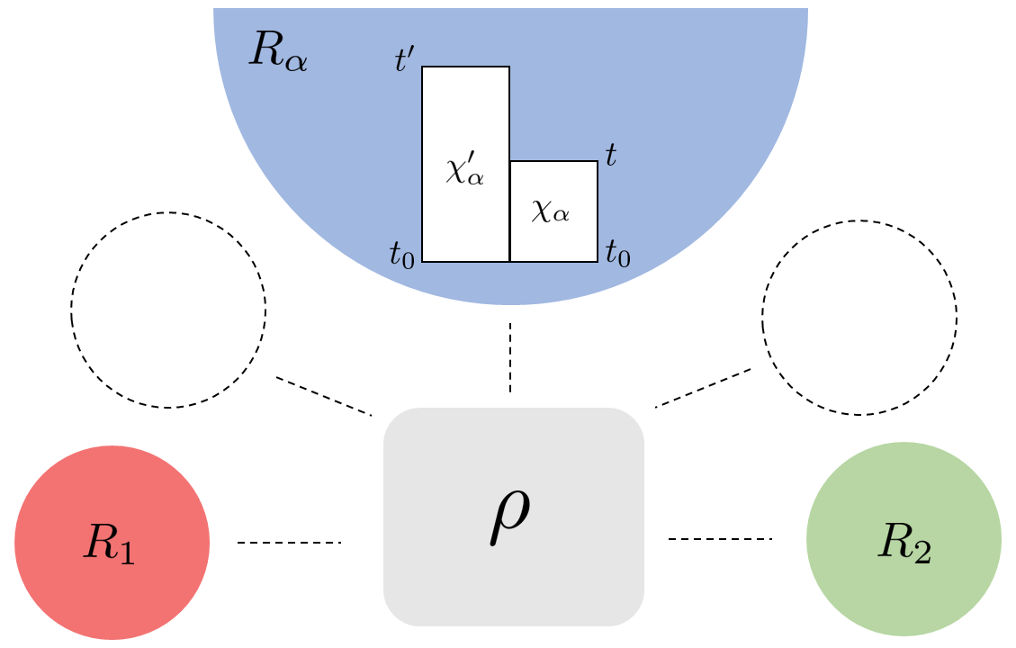
Figure 2: Scheme outlining the conceptual framework for counting statistics for multiple terminals and multiple times. In reservoir $R_{\alpha}$, distinct boxes represent different time bins, each associated with a specific counting field ($\chi_{\alpha}$ for $t-t_{0}$ and $\chi^{\prime}_{\alpha}$ for $t^{\prime}-t_{0}$). The joint probability of observing a net transfer of $x^{\prime}_{\alpha}$ quanta during the time $t^{\prime}-t_{0}$ is obtained by counting both fields, $\chi_{\alpha}+\chi_{\alpha}^{\prime}$, for the interval $t-t_{0}$, and solely $\chi_{\alpha}^{\prime}$ for $t^{\prime}-t$. Generalizing this approach to multiple terminals involves analogous operations with the vectors $\vec{\chi}$ and $\vec{\chi}^{\prime}$.

Notice that with $\vec{\chi}=0$, the above equation reduces to the standard form of Eq. (20), with $\mathcal{L}(\vec{\chi}=0)=\mathcal{L}$. The formal solution of Eq. (30) is given by,

$$\rho(\vec{\chi},t)=\Omega(\vec{\chi},t-t_{0})\rho(\vec{\chi},t_{0})=\Omega(\vec{\chi},t-t_{0})\rho_{0},$$ (32)

with $\rho_{0}=\rho(t_{0})$ the initial state of the system, and where we assumed no tunneling at time $t_{0}$, i. e. $\rho(\vec{\chi},t_{0})=\rho_{0}$.

In the above equation we introduced the propagator in $\vec{\chi}$-space $\Omega(\vec{\chi},t)=e^{\mathcal{L}(\vec{\chi})t}$. The propagator in the $\vec{x}$-space is simply given by the inverse Fourier transform $\Omega(\vec{x},t)=\int d\vec{\chi}/(2\pi)^{N}e^{-i\vec{x}\cdot\vec{\chi}}~{}\Omega(\vec{\chi},t)$, such that $\rho^{(\vec{x})}(t)=\Omega(\vec{x},t-t_{0})\rho_{0}$. The propagator in the $\vec{x}$-space is essential for computing the joint probability $P^{>}(\vec{x},t;\vec{x}^{\prime},t^{\prime})$ of having a net amount $\vec{x}$ of particles, charges, or energy quanta transferred within time $t-t_{0}$ and $\vec{x}^{\prime}$ within time $t^{\prime}-t_{0}$, where the superscript “$>$” indicates $t^{\prime}>t$. This joint probability is expressed as,

$$P^{>}(\vec{x},t;\vec{x}^{\prime},t^{\prime})=\Tr{\Omega(\vec{x}^{\prime}-\vec{x},t^{\prime}-t)\Omega(\vec{x},t-t_{0})\rho_{0}}.$$

The above expression can be derived using the Chapman–Kolmogorov property for Markovian evolution, as detailed in Appendix A, where we also provide a generalized multi-time expression. We note that the presented expression generalizes the two-time joint probability found in Refs. [44, 45], which was obtained under the conditions of a single terminal.

The joint probability of Eq. (II.2.1) is crucial for calculating average quantities within the master equation formalism, denoted as $\expectationvalue{\ldots}_{\text{ME}}$. For instance, the average number of tunneled particles, charges, or energy quanta exchanged with reservoir $\alpha$ within time $t^{\prime}-t_{0}$, can be expressed through the derivative of the joint probability with respect to the counting field, $\chi^{\prime}_{\alpha}$, as detailed in Appendix B,

$$\expectationvalue{x^{\prime}_{\alpha}(t^{\prime})}_{\text{ME}}=\int_{t_{0}}^{t^{\prime}}ds^{\prime}F(t^{\prime}-s^{\prime})\partial_{i\chi^{\prime}_{\alpha}}P^{>}(\vec{\chi},s;\vec{\chi}^{\prime},s^{\prime})\big{\rvert}_{\vec{\chi},\vec{\chi}^{\prime}=0}.$$ (34)

Here, the function $F$ serves as a detection response function, similar to ones introduced in the context of quantum optics [62, 63, 64], with boundary conditions $F(0)=F(t-t_{0})=0$  . In typical resources on FCS, the tunneling of quanta is assumed to be instantaneous, corresponding to the detection response function being a delta function, i.e. $F(t-s)=\delta(s-t)$ . In Eq.(34) we have introduced the joint probability in the $\vec{\chi}$-space,

$$P^{>}(\vec{\chi},t;\vec{\chi}^{\prime},t^{\prime})=\Tr{\Omega(\vec{\chi}^{\prime},t^{\prime}-t)\Omega(\vec{\chi}+\vec{\chi}^{\prime},t-t_{0})\rho_{0}}.$$ (35)

The expression can be intuitively understood using Fig. 2. The counting procedure involves first counting with both counting-field vectors $\vec{\chi}$ and $\vec{\chi}^{\prime}$ in the time-bin $t-t_{0}$ (i.e., evolving with $\Omega\left(\vec{\chi}+\vec{\chi}^{\prime},t-t_{0}\right)$) and then with just $\vec{\chi}^{\prime}$ in the time bin $t^{\prime}-t$ (i.e., evolving with $\Omega\left(\vec{\chi}^{\prime},t^{\prime}-t\right)$).

The average current associated to $x_{\alpha}(t)$ can now be calculated by taking the time derivative of Eq. (34). Utilizing the property of the derivative of a convolution product, the boundary conditions of $F$, and employing the trace-preserving property of the Lindbladian $\Tr{\mathcal{L}(0)\sigma}=0$ (valid for any operator $\sigma$), we obtain (see Appendix B for more details),

$$\partial_{t}\expectationvalue{x_{\alpha}(t)}_{\text{ME}}=\int_{t_{0}}^{t}ds\,F\left(t\!-\!s\right)\Tr\{\,\partial_{i\chi_{\alpha}}\mathcal{L}(\vec{\chi})\rvert_{\vec{\chi}=0}e^{\mathcal{L}\left(s-t_{0}\right)}\rho_{0}\},$$ (36)

where we have now changed primed labels to unprimed ones, for clarity. The particle and energy currents can be obtained from the above equation by considering $x_{\alpha}\equiv n_{\alpha}$ (with $\nu_{j\alpha}=1$) for the former, and $x_{\alpha}\equiv\epsilon_{\alpha}$ (with $\nu_{j\alpha}=\epsilon_{j}$) for the latter, see Eq. (28)

$$\left\langle I_{\alpha}(t)\right\rangle_{\text{ME}} = \int_{t_{0}}^{t}ds\,F\left(t-s\right)\Tr\{\mathcal{I}_{\alpha}e^{\mathcal{L}\left(s-t_{0}\right)}\rho_{0}\},$$ (37)

$$\left\langle J_{\alpha}(t)\right\rangle_{\text{ME}} = \int_{t_{0}}^{t}ds\,F\left(t-s\right)\Tr\{\mathcal{J}_{\alpha}e^{\mathcal{L}\left(s-t_{0}\right)}\rho_{0}\},$$ (38)

where we have introduced the particle current and energy current superoperators,

$$\mathcal{I}_{\alpha} \coloneqq\partial_{i\chi_{\alpha}}\mathcal{L}(\vec{\chi})\big{\rvert}_{\begin{subarray}{c}\vec{\chi}=0\\ \nu_{j\alpha}=1\end{subarray}}\,\,=\sum_{j}\left(\mathcal{L}_{j\alpha}^{+}-\mathcal{L}_{j\alpha}^{-}\right),$$ (39)

$$\mathcal{J}_{\alpha} \coloneqq\partial_{i\chi_{\alpha}}\mathcal{L}(\vec{\chi})\big{\rvert}_{\begin{subarray}{c}\vec{\chi}=0\\ \nu_{j\alpha}=\epsilon_{j}\end{subarray}}=\sum_{j}\epsilon_{j}\left(\mathcal{L}_{j\alpha}^{+}-\mathcal{L}_{j\alpha}^{-}\right).$$ (40)

The intuition behind the forms of these equations is self-evident; the superoperators count the net number of particles or the net amount of energy exchanged between the system and reservoir $\alpha$. It is important to note that Eqs. (37) and (38) are valid at all times, for any detection response function. To make a comparison with the usual master equation results, one may consider the case in which jumps happen instantaneously. In this case, $F(t-s)=\delta(s-t)$, and familiar expressions for the currents can be recovered, which we will refer to later in this work as $I^{\text{ME}}_{\alpha}$ and $J^{\text{ME}}_{\alpha}$, respectively,

$$I^{\text{ME}}_{\alpha}(t) =\Tr\left\{\mathcal{I}_{\alpha}\rho\left(t\right)\right\}=\Tr\left\{\mathcal{I}_{\alpha}e^{\mathcal{L}\left(t-t_{0}\right)}\rho_{0}\right\},$$ (41)

$$J^{\text{ME}}_{\alpha}(t) =\Tr\left\{\mathcal{J}_{\alpha}\rho\left(t\right)\right\}=\Tr\left\{\mathcal{J}_{\alpha}e^{\mathcal{L}\left(t-t_{0}\right)}\rho_{0}\right\}.$$ (42)

The above expressions coincide with those recently introduced in Ref. [39], derived within the framework of the stochastic master equation. Notably, our formalism allows us to obtain the same results without resorting to quantum stochastic principles.

Similarly to Eqs. (34), the above framework can be extended to calculate the two-time average,

$$\expectationvalue{x_{\alpha}(t)x^{\prime}_{\alpha^{\prime}}(t^{\prime})}_{\text{ME}} =\int_{t_{0}}^{t}ds\int_{t_{0}}^{t^{\prime}}ds^{\prime}F(t-s)F(t^{\prime}-s^{\prime})$$

$$\times\partial_{i\chi_{\alpha}}\partial_{i\chi^{\prime}_{\alpha^{\prime}}}P(\vec{\chi},s;\vec{\chi}^{\prime},s^{\prime})\big{\rvert}_{\vec{\chi},\vec{\chi}^{\prime}=0}$$ (43)

where we have introduced the time-ordered joint probability,

$$P(\vec{\chi},t;\vec{\chi}^{\prime},t^{\prime})= \Theta(t^{\prime}-t)P^{>}\left(\vec{\chi},t;\vec{\chi}^{\prime},t^{\prime}\right)$$

$$+ \Theta(t-t^{\prime})P^{<}\left(\vec{\chi},t;\vec{\chi}^{\prime},t^{\prime}\right)$$ (44)

with $P^{<}\left(\vec{\chi},t;\vec{\chi}^{\prime},t^{\prime}\right)=P^{>}\left(\vec{\chi}^{\prime},t^{\prime};\vec{\chi},t\right)$. Taking the double derivative of Eq. (II.2.1) with respect to times $t$ and $t^{\prime}$, and using $x_{\alpha},x^{\prime}_{\alpha^{\prime}}=n_{\alpha},n^{\prime}_{\alpha^{\prime}}$, we can compute the two-time current correlation, which takes the following form,

$$\left\langle I_{\alpha}(t)I_{\alpha^{\prime}}(t^{\prime})\right\rangle_{\text{ME}} =\partial_{t}\partial_{t^{\prime}}\int_{t_{0}}^{t}ds\int_{t_{0}}^{t^{\prime}}ds^{\prime}F(t-s)F(t^{\prime}-s^{\prime})\times\partial_{i\chi_{\alpha}}\partial_{i\chi^{\prime}_{\alpha^{\prime}}}P(\vec{\chi},s;\vec{\chi}^{\prime},s^{\prime})\big{\rvert}_{\vec{\chi},\vec{\chi}^{\prime}=0}$$

$$=\delta_{\alpha\alpha^{\prime}}\int_{t_{0}}^{t}ds\,F\left(t-s\right)F\left(t^{\prime}-s\right)\text{Tr}\{\mathcal{A}_{\alpha}\,e^{\mathcal{L}\left(t^{\prime}-t_{0}\right)}\rho_{0}\}$$

$$+\int_{t_{0}}^{t}ds\int_{t_{0}}^{t^{\prime}}ds^{\prime}F(t-s)F(t^{\prime}-s^{\prime})\Theta\left(s^{\prime}-s\right)\text{Tr}\{\mathcal{I}_{\alpha^{\prime}}e^{\mathcal{L}\left(s^{\prime}-s\right)}\mathcal{I}_{\alpha}\rho(s)\}$$

$$+\int_{t_{0}}^{t}ds\int_{t_{0}}^{t^{\prime}}ds^{\prime}F(t-s)F(t^{\prime}-s^{\prime})\Theta\left(s-s^{\prime}\right)\text{Tr}\{\mathcal{I}_{\alpha}e^{\mathcal{L}\left(s-s^{\prime}\right)}\mathcal{I}_{\alpha^{\prime}}\rho(s^{\prime})\}.$$ (45)

The detailed derivation of the expression above can be found in Appendix B. This expression, which agrees with the results of Ref. [64] obtained in the context of quantum optics, is composed of three terms. The last two terms contain the particle current superoperators $\mathcal{I}_{\alpha},\mathcal{I}_{\alpha^{\prime}}$, defined in Eq. (39). In the first term, we have identified the dynamical activity superoperator $\mathcal{A}_{\alpha}$ defined as [39],

$$\mathcal{A}_{\alpha}=-\partial^{2}_{\chi_{\alpha}}\mathcal{L}(\vec{\chi})\big{\rvert}_{\begin{subarray}{c}\vec{\chi}=0\\ \nu_{j\alpha}=1\end{subarray}}=\sum_{j}\left(\mathcal{L}_{j\alpha}^{+}+\mathcal{L}_{j\alpha}^{-}\right),$$ (46)

which is a measure of how frequently jumps occur between the system and the reservoir $\alpha$.

In the case of instantaneous jumps, the current correlation function within the master equation approach, denoted as $S^{\text{ME}}_{\alpha\alpha^{\prime}}(t,t^{\prime})$, is derived from Eq. (II.2.1) by substituting $F(t-s)=\delta(s-t)$ and subtracting the product of currents, $I_{\alpha}(t)^{\text{ME}}I_{\alpha^{\prime}}^{\text{ME}}(t^{\prime})$. The resulting expression simplifies to the following form,

$$S^{\text{ME}}_{\alpha\alpha^{\prime}}(t,t^{\prime}) =\delta_{\alpha\alpha^{\prime}}\delta(t-t^{\prime})\Tr{\mathcal{A}_{\alpha}e^{\mathcal{L}(t-t_{0})}\rho_{0}}$$

$$+\Theta(t^{\prime}-t)\Tr{\mathcal{I}_{\alpha^{\prime}}e^{\mathcal{L}(t^{\prime}-t)}\mathcal{I}_{\alpha}e^{\mathcal{L}(t-t_{0})}\rho_{0}}$$

$$+\Theta(t-t^{\prime})\Tr{\mathcal{I}_{\alpha}e^{\mathcal{L}(t-t^{\prime})}\mathcal{I}_{\alpha^{\prime}}e^{\mathcal{L}(t^{\prime}-t_{0})}\rho_{0}}$$

$$-\Tr{\mathcal{I}_{\alpha}e^{\mathcal{L}(t-t_{0})}\rho_{0}}\Tr{\mathcal{I}_{\alpha^{\prime}}e^{\mathcal{L}(t^{\prime}-t_{0})}\rho_{0}}.$$ (47)

The last line simply corresponds to the product of the average currents at leads $\alpha$ and $\alpha^{\prime}$ at times $t$ and $t^{\prime}$, respectively. The first line is proportional to a Dirac delta function which, in the Fourier domain will correspond to white noise: it is present at all frequencies with equal strength [39]. Due to the Kronecker delta, this term is present only for auto-correlations ($\alpha=\alpha^{\prime}$) and is zero for cross-correlations. The second and third lines can be obtained alternatively by applying the quantum regression theorem [67], while the first cannot. Overall, the above expression agrees with previous results obtained in different forms in the context of quantum stochastic master equation [64, 36, 68, 37, 39], all derived under the assumption of instantaneous jumps. In the following section, we will return to this important point, recovering the above expressions with a concrete example of a single-level quantum dot using exact principles.

II.3 Landauer-Büttiker approach

The Landauer-Büttiker (LB) [21, 22, 2, 40, 69] or scattering matrix (s-matrix) theory of transport provides a simple and powerful theoretical framework for the description of currents and current correlations in mesoscopic conductors, when coherent and elastic scattering processes are assumed in the active region. Under these conditions, the scattering formalism has been shown to be equivalent to the non-equilibrium Green’s function formalism [2]. However, in contrast to the Heisenberg equation and master equation approaches, the Landauer-Büttiker theory is restricted to steady-state observables and non-interacting quantum systems. Nevertheless, this framework accounts for arbitrary system-environment coupling strengths and allows for periodically-driven Hamiltonians [69]. Below, we briefly recall the central concepts of this approach, to fix the terms and notations. This preparatory step is essential as we subsequently delve into a specific example, utilizing the LB formalism to benchmark results against the HE and ME approaches.

As illustrated in Fig. 1 (c), the central object is the s-matrix $\mathcal{S}$, which relates the incoming and outgoing annihilation fermionic operators in the reservoirs, $\hat{b}_{\alpha}$ and $\hat{a}_{\alpha}$, respectively, with $\alpha=1,\ldots,N$. For a setup with $N$ reservoirs, and one transport channel per lead, it is therefore a $N\times N$ matrix with elements denoted $\mathcal{S}_{\alpha\beta}$, defined as,

$$\hat{b}_{\alpha}(\epsilon)=\sum_{\beta}\mathcal{S}_{\alpha\beta}(\epsilon)\hat{a}_{\beta}(\epsilon).$$ (48)

A corresponding equation establishes the connection between the creation operators $\hat{b}^{\dagger}_{\alpha}$ and $\hat{a}^{\dagger}_{\alpha}$ via $\mathcal{S}^{*}(\epsilon)$. Particle conservation is ensured through the unitarity of the s-matrix, $\mathcal{S}\mathcal{S}^{\dagger}=\mathcal{S}^{\dagger}\mathcal{S}=\mathds{1}$. The particle current operator can be expressed in terms of the s-matrix, and incoming and outgoing operators in the following way [40],

$$\hat{I}_{\alpha}^{LB}(t)=\!\!\int_{-\infty}^{\infty}\!\!\frac{d\epsilon~{}d\epsilon^{\prime}}{2\pi}e^{-i(\epsilon-\epsilon^{\prime})t}\left[\hat{a}_{\alpha}^{\dagger}(\epsilon)\hat{a}_{\alpha}(\epsilon^{\prime})-\hat{b}_{\alpha}^{\dagger}(\epsilon)\hat{b}_{\alpha}(\epsilon^{\prime})\right].$$ (49)

The average particle current is calculated by substituting Eq. (48) in the above expression, taking the statistical average, and using the relation $\expectationvalue{\hat{a}_{\alpha}^{\dagger}\left(\epsilon\right)\hat{a}_{\beta}\left(\epsilon^{\prime}\right)}=\delta_{\alpha\beta}\delta{\left(\epsilon-\epsilon^{\prime}\right)}f_{\alpha}\left(\epsilon\right)$, where $f_{\alpha}\left(\epsilon\right)$ is the Fermi-Dirac distribution function. The method explained so far is valid for an arbitrary number of reservoirs; however, simpler expressions for currents and current correlations can be obtained in the case of a two-terminal scenario, i.e., $\alpha=L,R$ (for left and right respectively). In this case, the average particle current in the steady state takes the form,

$$I^{\text{LB}}_{\alpha} =\sum_{\beta}\int\frac{d\epsilon}{2\pi}\mathcal{T}(\epsilon)\left(f_{\alpha}(\epsilon)-f_{\bar{\alpha}}(\epsilon)\right),$$ (50)

where $\bar{\alpha}$ denotes the opposite lead of $\alpha=L,R$, and where we introduced the so called transmission function $\mathcal{T}(\epsilon)=\absolutevalue{\mathcal{S}_{\alpha\bar{\alpha}}}^{2}$. Similarly we can obtain the energy current,

$$J^{\text{LB}}_{\alpha} =\int_{-\infty}^{\infty}\frac{d\epsilon}{2\pi}\,\epsilon\,\mathcal{T}(\epsilon)\left(f_{\alpha}(\epsilon)-f_{\bar{\alpha}}(\epsilon)\right),$$ (51)

which simply contains an extra energy term $\epsilon$ under the integral. These average currents correspond to the steady-state limit of the currents obtained from the HE approach, valid for all system-bath coupling strengths in the limit of $t\to\infty$. In the example of a single-level quantum dot treated in the following section, we will show how to take this limit explicitly.
The Landauer-Büttiker approach also enables the computation of the steady-state current correlation function. In the stationary regime, due to time-translation invariance, the current correlation function depends solely on the time difference, denoted as $S^{\text{LB}}_{\alpha\alpha^{\prime}}(\tau)$ with $\tau=t-t^{\prime}$. Furthermore, within the LB framework, it is customary to analyze the spectrum of $S^{\text{LB}}_{\alpha\alpha^{\prime}}(\omega)$ (also known as noise power), which corresponds to the Fourier transform [40],

$$S^{\text{LB}}_{\alpha\alpha^{\prime}}(\omega)=\int_{-\infty}^{\infty}d\tau e^{-i\omega\tau}S^{\text{LB}}_{\alpha\alpha^{\prime}}(\tau).$$ (52)

It can be shown that the finite-frequency noise satisfies $S_{\alpha\alpha^{\prime}}(\omega)=S_{\alpha^{\prime}\alpha}(-\omega)$. At zero frequency, the so-called shot noise takes the following simple form for the auto-correlation functions,

$$S_{LL}^{\text{LB}}(\omega=0) =S_{RR}^{\text{LB}}(\omega=0)$$

$$=\int\frac{d\epsilon}{2\pi}\mathcal{T}(\epsilon)\sum_{\beta=L,R}f_{\beta}(\epsilon)\left(1-f_{\beta}(\epsilon)\right)$$

$$+\mathcal{T}(\epsilon)(1-\mathcal{T}(\epsilon))\left(f_{L}(\epsilon)-f_{R}(\epsilon)\right)^{2}.$$ (53)

The auto- and cross-correlation functions are then connected via the following relation,

$$S_{\alpha\alpha}^{\text{LB}}(\omega=0) =-S^{\text{LB}}_{\alpha\beta}(\omega=0)\,,\quad\beta\neq\alpha\,.$$ (54)

Zero-frequency exact expressions for the multi-terminal case can be found in Refs. [70, 40].

In the subsequent sections, we will focus on the specific case of a single quantum dot coupled to two reservoirs. We will use the shot noise $S_{\alpha\alpha^{\prime}}^{\text{LB}}(\omega=0)$ derived from the LB approach to benchmark our steady-state expressions obtained from the exact HE approach for all system-reservoir coupling strengths, and from the ME approach for weak coupling.

In Table I, we summarize the main formal expressions of average currents and current correlation functions discussed so far. rowsep=5pt,colsep =5pt

Master Equation Γt ∼const.Γ→0 ← Heisenberg Equation t→∞→ Landauer Büttiker

I_α(t) Tr{I_αe^L (t-t_0)ρ_0} -i⟨[^H,^N_α]⟩ ∫dϵ2πT(f_α-f_¯α)

J_α(t) Tr{J_αe^L (t-t_0)ρ_0} -i⟨[^H,^H_R_α]⟩ ∫dϵ2πϵT(f_α-f_¯α)

S_αα^′(t,t^′) δ_αα^′ δ(t-t’) Tr(A_αe^L (t-t_0)ρ_0)+Θ(t’-t)Tr(I_α’ e^L (t’-t) I_α e^L (t-t_0)ρ_0)+Θ(t-t’)Tr(I_α e^L (t-t’) I_α’ e^L (t’-t_0)ρ_0)- Tr(I_αe^L (t-t_0)ρ_0)Tr(I_α’e^L (t’-t_0)ρ_0) ⟨^I_α(t)^I_α^′(t^′)⟩-⟨^I_α(t)⟩⟨^I_α^′(t^′)⟩ ∫dϵ2πT∑_βf_β(1-f_β)+T(1-T)(f_L-f_R)^2

Table 1: Different rows correspond to different observables: particle current ($I_{\alpha}$), energy current ($J_{\alpha}$), and current correlation fuction ($S_{\alpha\alpha^{\prime}}$). Different columns correspond to different approaches: master equation (ME), Heisenberg equation of motion (HE), and Landauer Büttiker (LB). Each entry in the table provides an expression for computing the corresponding quantity within the relevant framework. In the text, we explain how to obtain results in the ME and LB frameworks from the exact results obtained in the HE framework. This involves applying the weak-coupling protocol for the ME framework and taking the stationary limit $t\to\infty$ for the LB framework. Note that the expression for the correlation function in the LB regime corresponds to the zero-frequency component of the noise power, i.e. the shot noise given in Eq. (II.3).

III Application: The single-level quantum dot

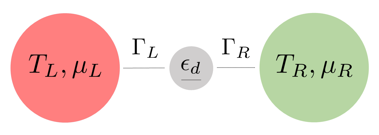
Figure 3: Scheme of the single-level quantum dot with energy $\epsilon_{d}$, coupled to two reservoirs at temperature $T_{\alpha}$ and chemical potential $\mu_{\alpha}$, with $\alpha=L,R$. In the WBL, $\Gamma_{L}$ and $\Gamma_{R}$ represent the energy-independent bare tunneling rates describing the coupling of the dot with the left and right reservoir respectively.

In this section, we analyze the specific case of a single-energy level quantum dot (QD) coupled with two reservoirs as depicted in Fig. 3. The Hamiltonian describing this system corresponds to the model introduced in Eq. (1) with $D=1$ and $N=2$. Specifically, by indicating with $\epsilon_{d}$ the energy of the dot, the Hamiltonian takes the following form,

$$\hat{H}=\epsilon_{d}\hat{d}^{\dagger}\hat{d}+\sum_{\alpha k}\epsilon_{k\alpha}\hat{c}_{k\alpha}^{\dagger}\hat{c}_{k\alpha}+\sum_{\alpha k}\left[t_{k\alpha}^{*}\hat{c}_{k\alpha}^{\dagger}\hat{d}+t_{k\alpha}\hat{d}^{\dagger}\hat{c}_{k\alpha}\right].$$ (55)

Each fermionic reservoir $\alpha=L,R$ is characterized by its Fermi-Dirac distribution, $f_{\alpha}(\epsilon)=\{e^{(\epsilon-\mu_{\alpha})/T_{\alpha}}+1\}^{-1}$, with $\mu_{\alpha}$ the chemical potential and $T_{\alpha}$ the temperature.

In the following, we start first by computing the exact expressions of currents and current correlation function obtained from the HE approach (Sec. IV), and benchmark them with the LB results in the steady-state regime (Sec. IV.2). Moving forward, in Sec. V, we present the results obtained from the ME approach. Finally, in Sec.VI, we delve into the discussion of the interconnections between these three frameworks, as outlined in Fig.1.

IV Heisenberg equation for the single-level QD

Inserting Eq. (55) into the Heisenberg equations Eqs. (5) and (6), we obtain the following evolution equations for the operators $d^{\dagger}$ and $c^{\dagger}_{k\alpha}$ in the case of the single-level QD [49, 30],

$$\frac{d}{dt}\hat{d}^{\dagger} = i[\hat{H},\hat{d}^{\dagger}]=i\epsilon_{d}\hat{d}^{\dagger}+i\sum_{k,\alpha}t_{k\alpha}^{*}\hat{c}_{k\alpha}^{\dagger}\,,$$

$$\frac{d}{dt}\hat{c}_{k\alpha}^{\dagger} = i[\hat{H},\hat{c}_{k\alpha}^{\dagger}]=i\epsilon_{k\alpha}\hat{c}_{k\alpha}^{\dagger}+it_{k\alpha}\hat{d}^{\dagger}\,.$$ (56)

The Heisenberg equations for $\hat{d}$ and $\hat{c}_{k\alpha}$ are simply the hermitian conjugate of the above. Similarly, by inserting Eq. (55) into Eqs. (10) and (11), we can compute the particle and energy currents,

$$I_{\alpha}^{\text{HE}}(t) = -2\text{Im}\left\{\sum_{k}t_{k\alpha}^{*}\expectationvalue{\hat{c}_{k\alpha}^{\dagger}(t)\hat{d}(t)}\right\},$$ (57)

$$J_{\alpha}^{\text{HE}}(t) = -2\text{Im}\left\{\sum_{k}\epsilon_{k\alpha}t_{k\alpha}^{*}\expectationvalue{\hat{c}_{k\alpha}^{\dagger}(t)\hat{d}(t)}\right\}.$$ (58)

The current correlation function is derived by substituting the particle current operator expression into the definition given in Eq. (15). Employing Wick’s theorem, it can be expressed as a sum of products of two-point correlators, as explained in Appendix E. The resulting form is as follows,

$$S^{\text{HE}}_{\alpha\alpha^{\prime}}(t,t^{\prime}) =-\sum_{kk^{\prime}}\left\{t_{k\alpha}^{*}t_{k^{\prime}\alpha^{\prime}}^{*}\expectationvalue{\hat{c}_{k\alpha}^{\dagger}(t)\hat{d}(t^{\prime})}\expectationvalue{\hat{d}(t)\hat{c}_{k^{\prime}\alpha^{\prime}}^{\dagger}(t^{\prime})}\right.$$

$$\left.-t_{k\alpha}^{*}t_{k^{\prime}\alpha^{\prime}}\expectationvalue{\hat{c}_{k\alpha}^{\dagger}(t)\hat{c}_{k^{\prime}\alpha^{\prime}}(t^{\prime})}\expectationvalue{\hat{d}(t)\hat{d}^{\dagger}(t^{\prime})}\right.$$

$$-\left.t_{k\alpha}t_{k^{\prime}\alpha^{\prime}}^{*}\expectationvalue{\hat{d}^{\dagger}(t)\hat{d}(t^{\prime})}\expectationvalue{\hat{c}_{k\alpha}(t)\hat{c}_{k^{\prime}\alpha^{\prime}}^{\dagger}(t^{\prime})}\right.$$

$$\left.+t_{k\alpha}t_{k^{\prime}\alpha^{\prime}}\expectationvalue{\hat{d}^{\dagger}(t)\hat{c}_{k^{\prime}\alpha^{\prime}}(t^{\prime})}\expectationvalue{\hat{c}_{k\alpha}(t)\hat{d}^{\dagger}(t^{\prime})}\right\}.$$

It is worth noting that while auto- ($\alpha=\alpha^{\prime}$) and cross- ($\alpha\neq\alpha^{\prime}$) correlations are related in the stationary regime according to Eq.(54), this relationship does not hold in general in the transient regime. Notably, as elucidated in Appendix E, the two-point correlators in the above expression correspond to lesser Green functions for the dot, reservoirs, or between the dot and reservoirs.

IV.1 HE exact solutions for the QD

In the rest of the work, analytical solutions are derived by assuming the wide-band limit (WBL) as discussed along with Eq. (8), which entails a broad spectral density of the reservoirs with respect to the energy scales of the open quantum system, $\Gamma_{\alpha}(\epsilon)\equiv\Gamma_{\alpha}$, with $\alpha=L,R$. We also define for convenience, the total tunneling rate,

$$\Gamma=\Gamma_{L}+\Gamma_{R}\,.$$ (60)

Within the WBL, we obtain the analytical formal solution of the coupled differential equations (IV), for the operator $\hat{d}^{\dagger}(t)$,

$$\hat{d}^{\dagger}(t) =e^{\left(-\frac{\Gamma}{2}+i\epsilon_{d}\right)(t-t_{0})}\hat{d}^{\dagger}(t_{0})+\!\int_{t_{0}}^{t}\!\!ds~{}e^{\left(-\frac{\Gamma}{2}+i\epsilon_{d}\right)\left(t-s\right)}\xi^{\dagger}(s),$$

and for $\hat{c}^{\dagger}_{k\alpha}(t)$,

$$\hat{c}_{k\alpha}^{\dagger}(t) =e^{i\epsilon_{k\alpha}(t-t_{0})}\hat{c}_{k\alpha}^{\dagger}(t_{0})+i\int_{t_{0}}^{t}ds~{}e^{i\epsilon_{k\alpha}(t-s)}t_{k\alpha}\hat{d}^{\dagger}(s)$$

$$=e^{i\epsilon_{k\alpha}(t-t_{0})}\hat{c}_{k\alpha}^{\dagger}(t_{0})$$

$$+i\int_{t_{0}}^{t}ds~{}e^{\left(-\frac{\Gamma}{2}+i\epsilon_{d}\right)(s-t_{0})}e^{i\epsilon_{k\alpha}(t-s)}t_{k\alpha}\hat{d}^{\dagger}(t_{0})$$

$$+i\int_{t_{0}}^{t}\!\!ds\int_{t_{0}}^{s}\!\!ds^{\prime}~{}e^{i\epsilon_{k\alpha}(t-s)}e^{\left(-\frac{\Gamma}{2}+i\epsilon_{d}\right)(s-s^{\prime})}t_{k\alpha}\xi^{\dagger}\left(s^{\prime}\right).$$

where we have introduced the function,

$$\xi^{\dagger}(t)=i\sum_{k\alpha}t_{k\alpha}^{*}e^{i\epsilon_{k\alpha}(t-t_{0})}\hat{c}_{k\alpha}^{\dagger}(t_{0}).$$ (63)

Additional details for the derivation of the above solutions can be found in Appendix. D. Let us note that similar expressions for this paradigmatic model were already discussed in Refs. [30, 71]. The solutions for $\hat{d}(t)$ and $\hat{c}_{k\alpha}(t)$ can be obtained by taking the hermitian conjugate of Eqs. (IV.1) and (IV.1), respectively. We now substitute the above solutions into Eqs. (57) and (58), and apply the initial conditions at time $t_{0}$: $\expectationvalue{\hat{c}_{k\alpha}^{\dagger}(t_{0})\hat{c}_{k^{\prime}\alpha^{\prime}}(t_{0})}=\delta_{k\alpha,k^{\prime}\alpha^{\prime}}f_{\alpha}(\epsilon_{k\alpha})$ and $\expectationvalue{\hat{d}^{\dagger}(t_{0})\hat{d}(t_{0})}=n_{d}$. We finally obtain the time-dependent expressions for the particle and energy currents,

$$I_{\alpha}^{\text{HE}}(t) = \Gamma_{\alpha}\sum_{\beta}\frac{\Gamma_{\beta}}{\Gamma}\left\{-n_{d}\,e^{-\Gamma\left(t-t_{0}\right)}+\left(A_{\alpha}^{0}-A_{\beta}^{0}\right)-e^{-\frac{\Gamma}{2}\left(t-t_{0}\right)}\left[A_{\beta}^{0}+B_{\alpha}^{0}-2B_{\beta}^{0}+C_{\alpha}^{0}\right]\right\}$$ (64)

$$J_{\alpha}^{\text{HE}}(t) = \Gamma_{\alpha}\sum_{\beta}\frac{\Gamma_{\beta}}{\Gamma}\left\{-\epsilon_{d}n_{d}\,e^{-\Gamma\left(t-t_{0}\right)}+\left(A_{\alpha}^{1}-A_{\beta}^{1}\right)-e^{-\frac{\Gamma}{2}\left(t-t_{0}\right)}\left[B_{\alpha}^{1}-B_{\beta}^{1}+C_{\alpha}^{1}\right]\right\},$$ (65)

with the definitions of the integrals,

$$A_{\gamma}^{m} \coloneqq\Gamma\int\frac{d\epsilon}{2\pi}\frac{(\epsilon+\epsilon_{d})^{m}}{\frac{\Gamma^{2}}{4}+\epsilon^{2}}f_{\gamma}(\epsilon+\epsilon_{d}),\quad m=0,1\,,$$ (66)

$$B_{\gamma}^{m} \coloneqq\Gamma\int\frac{d\epsilon}{2\pi}\frac{(\epsilon+\epsilon_{d})^{m}}{\frac{\Gamma^{2}}{4}+\epsilon^{2}}f_{\gamma}(\epsilon+\epsilon_{d})\cos\left(\epsilon\left(t-t_{0}\right)\right),$$ (67)

$$C_{\gamma}^{m} \coloneqq 2\int\frac{d\epsilon}{2\pi}\frac{(\epsilon+\epsilon_{d})^{m}}{\frac{\Gamma^{2}}{4}+\epsilon^{2}}f_{\gamma}(\epsilon+\epsilon_{d})\epsilon\sin\left(\epsilon\left(t-t_{0}\right)\right).$$ (68)

In Eqs. (64) and (65), the first term that depends on initial occupation of the dot $n_{d}$ corresponds to a shift in the current that decays exponentially in time. Since the steady state cannot depend on the initial state, the contribution of $n_{d}$ naturally has to be exponentially decaying. The second term, being independent of time, corresponds to the steady-state current. The third term is an oscillating, exponentially decaying contribution, which does not depend on the initial state of the system.

In Fig. 4, we illustrate the results of Eqs. (64) and (65) by plotting the particle and energy currents as functions of time, for various energies of the dot in panel (a), and fixed initial dot occupation $n_{d}=0$, and then for different $n_{d}$, for two values of dot energies in panel (b). We have considered the two reservoirs to be at the same temperature ($T_{L}=T_{R}$) with opposite chemical potentials ($\mu_{L}=-\mu_{R}$), such that the transport enegy window is symmetric around the zero energy. When the energy of the dot lies at the centre of the transport window ($\epsilon_{d}/\Gamma=0$), we find classical behaviour of the current, marked by exponential decay towards the steady state. However, as the energy of the dot moves away from the transport window, we start probing quantum coherent effects such as quantum tunnelling, seen clearly in the form of oscillations in the current at large $\epsilon_{d}$. Interestingly, such behaviour cannot be seen with the master equation approach, which only involves simple exponential decay toward the steady state, as we will see in the next section on ME.

For the current correlation function, we proceed in a similar way as for the currents. We insert Eqs. (IV.1) and (IV.1) into Eq. (IV). A long calculation leads to the following exact analytical expression of $S^{\text{HE}}_{\alpha\alpha^{\prime}}(t,t^{\prime})$, valid at all times,

$$S^{\text{HE}}_{\alpha\alpha^{\prime}}(t,t^{\prime}) =\Gamma_{\alpha}\Gamma_{\alpha^{\prime}}\sum_{\beta,\beta^{\prime}}\frac{\Gamma_{\beta}\Gamma_{\beta^{\prime}}}{\Gamma^{2}}\left[\Lambda_{0}(t,t^{\prime})-\Lambda^{-}_{\alpha}(t,t^{\prime})+\Lambda^{\pm}_{\beta}(t,t^{\prime})\right]\left[\overline{\Lambda}_{0}(t^{\prime},t)-\overline{\Lambda}^{-}_{\alpha^{\prime}}(t^{\prime},t)+\overline{\Lambda}^{\pm}_{\beta^{\prime}}(t^{\prime},t)\right]$$

$$+\Gamma_{\alpha}\Gamma_{\alpha^{\prime}}\sum_{\beta,\beta^{\prime}}\frac{\Gamma_{\beta}\Gamma_{\beta^{\prime}}}{\Gamma^{2}}\left[\Lambda_{0}(t,t^{\prime})-\Lambda^{-}_{\alpha}(t,t^{\prime})-\Lambda^{-}_{\alpha^{\prime}}(t^{\prime},t)^{*}+\Lambda^{\pm}_{\beta}(t,t^{\prime})\right]\left[\overline{\Lambda}_{0}(t^{\prime},t)+\overline{\Lambda}^{\pm}_{\beta^{\prime}}(t^{\prime},t)\right]$$

$$+\Gamma_{\alpha}\delta_{\alpha\alpha^{\prime}}\sum_{\beta}\Gamma_{\beta}\Lambda_{\alpha}(t,t^{\prime})\left[\overline{\Lambda}_{0}(t^{\prime},t)+\overline{\Lambda}^{\pm}_{\beta}(t^{\prime},t)\right]+\left\{c.c.\quad\text{with}\quad\Lambda\leftrightarrow\overline{\Lambda}\right\},$$ (69)

with the definitions,

$$\Lambda_{0}(t,t^{\prime})=\frac{1}{2}e^{-\frac{\Gamma}{2}(t+t^{\prime})}e^{\Gamma t_{0}}e^{i\epsilon_{0}(t-t^{\prime})}n_{d}$$ (70)

$$\Lambda_{\gamma}(t,t^{\prime})=\frac{2}{\Gamma}\int\!\frac{d\epsilon}{2\pi}e^{i\epsilon\left(t-t^{\prime}\right)}f_{\gamma}\left(\epsilon\right)$$

$$\Lambda^{-}_{\gamma}(t,t^{\prime})=2\int\!\frac{d\epsilon}{2\pi}e^{i\epsilon\left(t-t^{\prime}\right)}g_{-}(\epsilon-\epsilon_{d},t)f_{\gamma}\left(\epsilon\right)$$

$$\Lambda^{\pm}_{\gamma}(t,t^{\prime})=2\Gamma\!\!\int\!\!\frac{d\epsilon}{2\pi}e^{i\epsilon\left(t-t^{\prime}\right)}g_{-}(\epsilon-\epsilon_{d},t)g_{+}(\epsilon-\epsilon_{d},t^{\prime})f_{\gamma}(\epsilon),$$

and,

$$g_{\pm}(\epsilon,t)=\frac{e^{-\left(\frac{\Gamma}{2}\pm i\epsilon\right)\frac{t-t_{0}}{2}}}{\frac{\Gamma}{2}\pm i\epsilon}\sinh{\left[\left(\frac{\Gamma}{2}\pm i\epsilon\right)\frac{t-t_{0}}{2}\right]},$$ (71)

where the $\overline{\Lambda}$ functions are obtained from Eqs. (70) substituting $n_{d}\rightarrow(1-n_{d})$ and $f_{\gamma}\left(\epsilon\right)\rightarrow\left(1-f_{\gamma}\left(\epsilon\right)\right)$. Let us remark that this general exact expression of the correlation function is complex and satisfies the relation $S_{\alpha\alpha^{\prime}}(t,t^{\prime})=S^{*}_{\alpha^{\prime}\alpha}(t^{\prime},t)$.

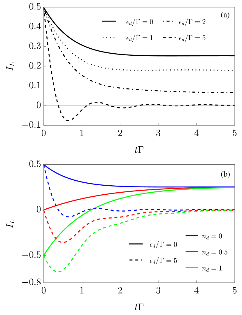
Figure 4: Particle current as a function of $t\Gamma$ with (a) constant $n_{d}=0$ and different values of $\epsilon_{d}/\Gamma=0,\,1,\,2,\,5$, and (b) with different values of $n_{d}=0,\,0.5,\,1$ and two values of $\epsilon_{d}/\Gamma=0,\,5$. The other parameters are $\Gamma_{L}=\Gamma_{R}=1$, $\mu_{L}=-\mu_{R}=\Gamma/2$ and $T_{L}=T_{R}=\Gamma/100$ ($\hbar,k_{B}=1$).

We note that the above expression of the correlation function can equivalently be obtained using non-equilibrium Green’s function techniques in the Schwinger-Keldysh theory [72], as explained in Ref. [34]. Our expression (IV.1) singles out the explicit time-dependence of each term through the Lambda functions defined in Eq. (70), as well as the dependence on the coupling rates. This considerably simplifies the calculations of the long-time limit of the current correlation functions as discussed below, and simplifies applying the weak-coupling protocol to connect HE and ME frameworks, as presented in Sec. VI.

IV.2 Steady-state limit: Benchmark with LB

In this section, we recall known expressions from the LB approach for the steady-state particle and energy currents, as well as for the shot noise, for the single-level QD in a two-terminal setup. These expressions will then be used to benchmark the exact results in the steady state obtained from the HE in the previous section. As discussed in Sec. II.3, the key quantity of interest in the LB approach is the transmission probability, which has to be computed explicitly. Although its expression is known for this simple model, we provide details on its derivation in Appendix C. It takes the following form [73, 22, 74, 2],

$$\mathcal{T}\left(\epsilon\right)=\frac{\Gamma_{L}\Gamma_{R}}{\frac{\Gamma^{2}}{4}+(\epsilon-\epsilon_{d})^{2}},$$ (72)

and corresponds to a Lorentzian centered around the energy of the dot $\epsilon_{d}$, with a width set by the total tunneling rate $\Gamma=\Gamma_{L}+\Gamma_{R}$. Inserting $\mathcal{T}(\epsilon)$ into Eqs. (50) and (51), we obtain the well-known expressions,

$$I_{L}^{\text{LB}} =\!\!-I_{R}^{\text{LB}}=\!\!\int\frac{d\epsilon}{2\pi}\frac{\Gamma_{L}\Gamma_{R}}{\frac{\Gamma^{2}}{4}+(\epsilon-\epsilon_{d})^{2}}\big{(}f_{L}(\epsilon)\!\!-f_{R}(\epsilon)\big{)},$$ (73)

$$J_{L}^{\text{LB}} =\!\!-J_{R}^{\text{LB}}=\!\!\int\frac{d\epsilon}{2\pi}\frac{\epsilon\,\Gamma_{L}\Gamma_{R}}{\frac{\Gamma^{2}}{4}+(\epsilon-\epsilon_{d})^{2}}\big{(}f_{L}(\epsilon)\!\!-f_{R}(\epsilon)\big{)}.$$ (74)

IV.2.1 Benchmarking with LB

To benchmark the exact results we obtained within the HE approach, we take the limit $t\rightarrow\infty$ (or equivalently taking $t_{0}\rightarrow-\infty$) in Eqs. (64) and (65). In this limit, all terms proportional to exponential time-decaying functions vanish, which lead us to the compact expressions,

$$I_{\alpha,ss}^{\text{HE}}\equiv\lim_{t\to\infty}I_{\alpha}^{\text{HE}}(t) =\Gamma_{\alpha}\sum_{\beta}\frac{\Gamma_{\beta}}{\Gamma}\left[A_{\alpha}^{0}-A_{\beta}^{0}\right],$$ (75)

$$J_{\alpha,ss}^{\text{HE}}\equiv\lim_{t\to\infty}J_{\alpha}^{\text{HE}}(t) =\Gamma_{\alpha}\sum_{\beta}\frac{\Gamma_{\beta}}{\Gamma}\left(A_{\alpha}^{1}-A_{\beta}^{1}\right).$$ (76)

It is simple to show that, by substituting the integrals $A_{\gamma}^{0},A_{\gamma}^{1}$ defined in Eq. (66), in the above equations and by performing the change of variable $\epsilon\to(\epsilon-\epsilon_{d})$, we recover the well-known expressions for the steady-state particle and energy currents in the reservoir $\alpha=L,R$ for a single-level QD in a two-terminal setup, coinciding exactly with Eqs. (73)-(74),

$$I_{\alpha,ss}^{\text{HE}} =I_{\alpha}^{\text{LB}}\quad\text{and}\quad J_{\alpha,ss}^{\text{HE}}=J_{\alpha}^{\text{LB}}.$$ (77)

Similarly to the average currents, the long-time limit of the current fluctuation functions $S^{\text{HE}}_{\alpha\alpha^{\prime},ss}$ is obtained by taking the limit $t\rightarrow\infty$ in Eqs. (70),

$$\lim_{t\to\infty}\Lambda_{0}(t,t^{\prime})=0,$$ (78)

$$\lim_{t\to\infty}\Lambda^{-}_{\gamma}(t,t^{\prime})=\int\frac{d\epsilon}{2\pi}\frac{e^{i\epsilon(t-t^{\prime})}}{\frac{\Gamma}{2}-i(\epsilon-\epsilon_{d})}f_{\gamma}(\epsilon),$$

$$\lim_{t\to\infty}\Lambda^{\pm}_{\gamma}(t,t^{\prime})=\frac{\Gamma}{2}\int\frac{d\epsilon}{2\pi}\frac{e^{i\epsilon(t-t^{\prime})}}{\frac{\Gamma^{2}}{4}+(\epsilon-\epsilon_{d})^{2}}f_{\gamma}(\epsilon),$$

$$\lim_{t\to\infty}\Lambda_{\gamma}(t,t^{\prime})=\frac{2}{\Gamma}\int\frac{d\epsilon}{2\pi}f_{\gamma}\left(\epsilon\right)e^{i\epsilon(t-t^{\prime})}\,.$$

The above functions only depend on the time difference $\tau=t-t^{\prime}$, as expected in the steady-state regime. We then substitute the above expressions into Eq. (IV.1), and take the Fourier transform with respect to the time delay $\tau$. In the next step, one has to exploit the convolution theorem to get an exact expression for the finite-frequency auto- and cross-current correlations,

$$\small S^{\text{HE}}_{\alpha\alpha^{\prime},ss}(\omega) =\frac{\Gamma_{\alpha}\Gamma_{\alpha^{\prime}}}{4\Gamma^{2}}\sum_{\beta,\beta^{\prime}}\Gamma_{\beta}\Gamma_{\beta^{\prime}}\int\frac{d\epsilon^{\prime}}{2\pi}\left[\frac{\Gamma f_{\beta}(\epsilon^{\prime})}{\frac{\Gamma^{2}}{4}+(\epsilon^{\prime}-\epsilon_{d})^{2}}-\frac{2f_{\alpha}(\epsilon^{\prime})}{\frac{\Gamma}{2}-i(\epsilon^{\prime}-\epsilon_{d})}\right]\left[\frac{\Gamma(1-f_{\beta^{\prime}}(\epsilon^{\prime}-\omega))}{\frac{\Gamma^{2}}{4}+(\epsilon^{\prime}-\omega-\epsilon_{d})^{2}}-\frac{2(1-f_{\alpha^{\prime}}(\epsilon^{\prime}-\omega))}{\frac{\Gamma}{2}-i(\epsilon^{\prime}-\omega-\epsilon_{d})}\right]$$

$$+\int\frac{d\epsilon^{\prime}}{2\pi}\sum_{\beta\beta^{\prime}}\frac{\Gamma_{\alpha}\Gamma_{\alpha^{\prime}}\Gamma_{\beta}\Gamma_{\beta^{\prime}}}{4\Gamma^{2}}\left[\frac{\Gamma f_{\beta^{\prime}}(\epsilon^{\prime})}{\frac{\Gamma^{2}}{4}+(\epsilon^{\prime}-\epsilon_{d})^{2}}-\frac{2f_{\alpha^{\prime}}(\epsilon^{\prime})}{\frac{\Gamma}{2}+i(\epsilon^{\prime}-\epsilon_{d})}-\frac{2f_{\alpha}(\epsilon^{\prime})}{\frac{\Gamma}{2}-i(\epsilon^{\prime}-\epsilon_{d})}\right]\frac{\Gamma(1-f_{\beta^{\prime}}(\epsilon^{\prime}-\omega))}{\frac{\Gamma^{2}}{4}+(\epsilon^{\prime}-\omega-\epsilon_{d})^{2}}$$

$$+\int\frac{d\epsilon^{\prime}}{2\pi}\sum_{\beta}\frac{\Gamma_{\alpha}\Gamma_{\beta}}{2\Gamma}\frac{\Gamma f_{\alpha}(\epsilon^{\prime})(1-f_{\beta}(\epsilon^{\prime}-\omega))}{\frac{\Gamma^{2}}{4}+(\epsilon^{\prime}-\omega-\epsilon_{d})^{2}}\delta_{\alpha\alpha^{\prime}}\quad+\left\{c.c.\quad\text{with}\quad f_{\gamma}\rightarrow\left(1-f_{\gamma}\right),~{}n_{d}\rightarrow\left(1-n_{d}\right)\right\}.$$ (79)

We verified that the above expression satisfies the well-known symmetry property $S^{\text{HE}}_{\alpha\alpha^{\prime},ss}(\omega)=S^{\text{HE}}_{\alpha^{\prime}\alpha,ss}(-\omega)$ [40]. The zero-frequency noise can be calculated from the above expression by taking $\omega=0$. By recognizing the transmission probability $\mathcal{T}(\epsilon)$ of Eq. (72), we can show that the shot noise coincides with the one obtained within the LB approach, as given in Eq. (II.3),

$$S^{\text{HE}}_{\alpha\alpha^{\prime},ss}(\omega=0)=S^{\text{LB}}_{\alpha\alpha^{\prime}}(\omega=0).$$ (80)

From the above result, we can verify that the zero-frequency cross and auto-correlation functions in a two-terminal setup satisfy $S_{RL}=S_{LR}=-S_{RR}=-S_{LL}$. We also note that, as expected, the zero-frequency components of the noise are real, the imaginary part cancels out. Overall, the results obtained in Eqs. (77) and (80), demonstrate the connection between the HE and LB pictures, as shown in Fig. 1 panels (a) to (c).

V Master equation for the QD

For a single-level QD in the ME formalism, it is convenient to express $\hat{H}_{S}=\epsilon_{d}\hat{d^{\dagger}}\hat{d}$ in terms of the raising and lowering operators for a two-level system in the canonical basis $\{\ket{0},\ket{1}\}$, namely $\sigma_{+}=\outerproduct{1}{0}$ and $\sigma_{-}=\outerproduct{0}{1}$ respectively. In this way, we can associate the operator $\hat{d}^{\dagger}$ ($\hat{d}$) to the operator $\sigma_{+}$ ($\sigma_{-}$). The Lindblad equation for this model is given by [28],

$$\dot{\rho}(t)=\mathcal{L}\,\rho(t)=\left(\mathcal{L}_{0}+\sum_{\alpha}(\mathcal{L}^{+}_{\alpha}+\mathcal{L}^{-}_{\alpha})\right)\rho(t).$$ (81)

Here, $\mathcal{L}_{0}$, defined in Eq. (21), takes the following form in terms of the non-hermitian commutator,

$$\mathcal{L}_{0}\rho=-i\left[\epsilon_{d}\sigma_{+}\sigma_{-}\!\!-\frac{i}{2}\sum_{\alpha}\left(\Gamma_{\alpha}^{-}\sigma_{+}\sigma_{-}+\Gamma_{\alpha}^{+}\sigma_{-}\sigma_{+}\right),\rho\right]_{\dagger}$$ (82)

and the Lindblad jump superoperators defined in Eqs. (22) and (23), are given by,

$$\mathcal{L}_{\alpha}^{+}\rho=\Gamma_{\alpha}^{+}\sigma_{+}\rho\sigma_{-},$$ (83)

$$\mathcal{L}_{\alpha}^{-}\rho=\Gamma_{\alpha}^{-}\sigma_{-}\rho\sigma_{+}.$$ (84)

V.1 Solution for $\rho(t)$

In order to compute observables within the ME approach, the time-dependent solution for the reduced density operator satisfying Eq. (81) is required. Although this is not a trivial task in general, analytical results can be obtained in the case of the single-level QD setup [30]. In this minimal model, no quantum coherences are formed during the dynamics, and only the populations for the ground and excited states are non-zero. Thus, assuming zero coherence at time $t_{0}$, the reduced density matrix of the system takes a diagonal form, $\rho(t)=\outerproduct{0}{0}p_{0}(t)+\outerproduct{1}{1}p_{1}(t)$, and the Lindblad master equation (81) reduces to the following rate equation for the populations, $\dot{p}_{i}=\sum_{j}W_{ij}p_{j}$, or explicitly,

$$\begin{pmatrix}\dot{p}_{0}\\ \dot{p}_{1}\end{pmatrix}=\left(\begin{array}[]{cc}-\Gamma_{L}^{+}-\Gamma_{R}^{+}&\Gamma_{L}^{-}+\Gamma_{R}^{-}\\ \Gamma_{L}^{+}+\Gamma_{R}^{+}&-\Gamma_{L}^{-}-\Gamma_{R}^{-}\\ \end{array}\right)\begin{pmatrix}p_{0}\\ p_{1}\end{pmatrix}.$$ (87)

Here, the elements $W_{ij}$ of the $2\times 2$ matrix $W$ are the transition rates from state $j$ to state $i$ (where $i,j=0,1$). The solution for $p_{1}(t)$ is given by,

$$p_{1}(t) =\sum_{\alpha}\frac{\Gamma_{\alpha}}{\Gamma}\left[f_{\alpha}+(f_{\alpha}-n_{d})e^{-\Gamma(t-t_{0})}\right].$$ (88)

with initial occupation probability $p_{1}(t_{0})=n_{d}$ at time $t=t_{0}$. The solution for the ground state is $p_{0}(t)=1-p_{1}(t)$, due to the conservation of probability. For convenience, we have used the notation $f_{\alpha}\coloneqq f_{\alpha}(\epsilon_{d})$, where the Fermi-Dirac distributions are evaluated at the energy of the dot $\epsilon_{d}$, a consequence of the weak-coupling assumption. Interestingly, this solution explicitly depends on the occupation imbalance between both reservoirs and the dot through the factor $\left(f_{\alpha}-n_{d}\right)$, which exponentially decays for long time.

V.2 Particle and energy currents with ME

Particle and energy current superoperators in reservoir $\alpha=L,R$ can be directly calculated from their definitions in Eqs. (39) and (40), using the explicit expressions of the Lindblad jump superoperators for a single-level QD given in Eq. (23). They take the following form,

$$\mathcal{I}_{\alpha}\rho =\left(\mathcal{L}_{\alpha}^{+}-\mathcal{L}_{\alpha}^{-}\right)\rho=\Gamma_{\alpha}^{+}\sigma_{+}\rho\sigma_{-}-\Gamma_{\alpha}^{-}\sigma_{-}\rho\sigma_{+},$$ (89)

$$\mathcal{J}_{\alpha}\rho =\epsilon_{d}\!\left(\mathcal{L}_{\alpha}^{+}-\mathcal{L}_{\alpha}^{-}\right)\rho=\epsilon_{d}\!\left(\Gamma_{\alpha}^{+}\sigma_{+}\rho\sigma_{-}\!\!-\Gamma_{\alpha}^{-}\sigma_{-}\rho\sigma_{+}\right)\!.$$ (90)

These superoperators reflect the positive (negative) count of particle or energy entering (leaving) the system, proportional to the rate $\Gamma_{\alpha}^{+}$ ($\Gamma_{\alpha}^{-}$). By inserting the above expressions of the currents superoperators into Eqs. (41), and using the time-dependent solution of the reduced density matrix of the system $\rho(t)$ of Eq. (88), we obtain the following analytical expressions for the particle and energy current,

$$I_{\alpha}^{\text{ME}}(t) =\Tr{\mathcal{I}_{\alpha}\rho(t)}$$

$$=\sum_{\beta}\frac{\Gamma_{\alpha}\Gamma_{\beta}}{\Gamma}\left[\left(f_{\alpha}-f_{\beta}\right)+\left(f_{\beta}-n_{d}\right)e^{-\Gamma(t-t_{0})}\right],$$ (91)

$$J_{\alpha}^{\text{ME}}(t) =\Tr{\mathcal{J}_{\alpha}\rho(t)}=\epsilon_{d}I_{\alpha}^{\text{ME}}(t).$$ (92)

The steady-state expressions can be calculated directly by taking the limit $t\rightarrow\infty$. In this case, the time-dependent part decays exponentially, and as expected the stationary part only depends on the difference of the Fermi-Dirac functions. In contrast, in the HE results, we saw a stationary part, an exponentially decaying part, as well as an oscillating exponentially decaying term.

V.3 Comment on the activity $\mathcal{A}$

The definition of the activity superoperator $\mathcal{A}$ comes naturally when deriving the exact expression for the current correlation function as discussed in Sec. II.2.1. The average activity $A_{\alpha}\coloneqq\Tr{\mathcal{A}_{\alpha}\rho}$ can be interpreted as the sum of all quantum jumps between reservoir $\alpha$ and the quantum system [39]. It provides information about the dynamics of the quantum system, and has recently been shown to be of utility to derive lower bounds for signal-to-noise ratio in the context of thermodynamic uncertainty relations [75, 76, 77]. In the case of the single-level QD, the activity superoperators in reservoir $\alpha=L,R$, can be made explicit by using the expressions of the Lindblad jump superoperators given in Eq. (23),

$$\mathcal{A}_{\alpha}\rho =\left(\mathcal{L}_{\alpha}^{+}+\mathcal{L}_{\alpha}^{-}\right)\rho=\Gamma_{\alpha}^{+}\sigma_{+}\rho\sigma_{-}+\Gamma_{\alpha}^{-}\sigma_{-}\rho\sigma_{+}\,.$$ (93)

As done for the currents, its average value can be computed using the time-dependent solution of the reduced density matrix of the system $\rho(t)$ of Eq. (88),

$$A_{\alpha}(t) \coloneqq\Tr{\mathcal{A}_{\alpha}\rho(t)}$$

$$=\sum_{\beta}\frac{\Gamma_{\alpha}\Gamma_{\beta}}{\Gamma}\left\{e^{-\Gamma t}\left(f_{\beta}-n_{d}\right)\left[f_{\alpha}-(1-f_{\alpha})\right]\right.$$

$$+\left.\left[f_{\beta}\left(1-f_{\alpha}\right)+f_{\alpha}\left(1-f_{\beta}\right)\right]\right\}.$$ (94)

A particularly intuitive interpretation of the above expression becomes apparent in the stationary limit as $t\to\infty$, where the steady-state activity takes the following form,

$$A_{\alpha,ss} =\lim_{t\to\infty}A_{\alpha}(t)$$

$$=\sum_{\beta}\frac{\Gamma_{\alpha}\Gamma_{\beta}}{\Gamma}\left[f_{\beta}\left(1-f_{\alpha}\right)+f_{\alpha}\left(1-f_{\beta}\right)\right].$$ (95)

The components of this expression have a natural interpretation. First, there is an overall factor, $\Gamma_{\alpha}\Gamma_{\beta}/\Gamma$, which is the probability of particle exchange between reservoirs $\alpha$ and $\beta$. The terms in the bracket, such as $f_{\alpha/\beta}\left(1-f_{\beta/\alpha}\right)$ for $\alpha,\beta=L,R$ can be interpreted in terms of the occupation or de-occupation of the dots. These terms represent the product of the probability that the incoming particle (toward the system) occupies the energy level of the dot in the lead $\alpha/\beta$ ($f_{\alpha/\beta}$) multiplied by the probability that the arriving energy level in the reservoir $\beta/\alpha$ is available (empty, i.e., $(1-f_{\beta/\alpha})$). They are reminiscent of the contributions to noise in the Landauer-Büttiker approach [40].

In addition to this formal derivation, it is important to note that the average activity $A_{\alpha}$, for a single-level QD in absence of quantum coherence can also be calculated directly using the rate matrix $W$ of Eq. (87) [77],

$$A_{\alpha}(t) = \sum_{i\neq j}(W_{\alpha})_{ij}p_{j}(t)\,.$$ (96)

Inserting the solution for $p_{1}(t)$ and $p_{0}(t)=1-p_{1}(t)$ from Eq. (88), in the above relation, it is easy to show that expressions in Eqs. (V.3) and (96) are equivalent.

V.4 Current correlation function with ME

The current correlation function for the single-level QD can be computed by inserting the expressions of the superoperators $\mathcal{I}_{\alpha},\mathcal{A}_{\alpha}$ and the solution $\rho(t)$ into Eq. (II.2.1),

$$S^{\text{ME}}_{\alpha\alpha^{\prime}}(t,t^{\prime}) = \delta_{\alpha\alpha^{\prime}}\delta(t-t^{\prime})\sum_{\beta}\frac{\Gamma_{\alpha}\Gamma_{\beta}}{\Gamma}\left\{e^{-\Gamma t}\left(f_{\beta}-n_{d}\right)\left[f_{\alpha}-(1-f_{\alpha})\right]+\left[f_{\beta}\left(1-f_{\alpha}\right)+f_{\alpha}\left(1-f_{\beta}\right)\right]\right\}$$ (97)

$$-\frac{e^{-\Gamma(t-t^{\prime})}}{\Gamma^{2}}\sum_{\beta,\beta^{\prime}}\Gamma_{\alpha}\Gamma_{\alpha^{\prime}}\Gamma_{\beta}\Gamma_{\beta^{\prime}}e^{-\Gamma t^{\prime}}\left(f_{\beta}-n_{d}\right)\left\{\left[(f_{\alpha}-f_{\beta^{\prime}})+(f_{\alpha^{\prime}}-f_{\beta^{\prime}})+(f_{\alpha^{\prime}}-f_{\alpha})\right]+e^{-\Gamma t^{\prime}}(f_{\beta^{\prime}}-n_{d})\right\}$$

$$-\frac{e^{-\Gamma(t-t^{\prime})}}{\Gamma^{2}}\sum_{\beta,\beta^{\prime}}\Gamma_{\alpha}\Gamma_{\alpha^{\prime}}\Gamma_{\beta}\Gamma_{\beta^{\prime}}\left[(1-f_{\beta})f_{\alpha^{\prime}}+f_{\beta}(f_{\beta^{\prime}}-f_{\alpha^{\prime}})\right]\,.$$

In the above, we have assumed $t>t^{\prime}$. Similar to the currents, all Fermi-Dirac distributions are evaluated at the energy of the dot $\epsilon_{d}$. By using the general relation $S_{\alpha\alpha^{\prime}}(t,t^{\prime})=S^{*}_{\alpha^{\prime}\alpha}(t^{\prime},t)$ [34], and exploiting the fact that the current correlation is real in the weak-coupling regime, Eq. (97) can be written for $t<t^{\prime}$ by exchanging $\alpha\leftrightarrow\alpha^{\prime}$ and $t\leftrightarrow t^{\prime}$.

In the steady state, we can obtain the analytical expression of the stationary noise in the weak-coupling regime, which only depends on the time difference $\tau=t-t^{\prime}$,

$$S^{\text{ME}}_{\alpha\alpha^{\prime},ss}(\tau) =\lim_{t\to\infty}S^{\text{ME}}_{\alpha\alpha^{\prime}}(t,t+\tau)$$

$$=\frac{\delta(\tau)\delta_{\alpha\alpha^{\prime}}}{\Gamma}\sum_{\beta}\Gamma_{\alpha}\Gamma_{\beta}\left\{f_{\beta}(\epsilon_{d})\left(1-f_{\alpha}(\epsilon_{d})\right)+f_{\alpha}(\epsilon_{d})\left(1-f_{\beta}(\epsilon_{d})\right)\right\}$$

$$-\frac{e^{-\Gamma\absolutevalue{\tau}}}{\Gamma^{2}}\sum_{\beta,\beta^{\prime}}\Gamma_{\alpha}\Gamma_{\alpha^{\prime}}\Gamma_{\beta}\Gamma_{\beta^{\prime}}\left\{\left(1-f_{\beta}(\epsilon_{d})\right)\left[f_{\alpha}(\epsilon_{d})\Theta(-\tau)+f_{\alpha^{\prime}}(\epsilon_{d})\Theta(\tau)\right]\right\}$$

$$-\frac{e^{-\Gamma\absolutevalue{\tau}}}{\Gamma^{2}}\sum_{\beta,\beta^{\prime}}\Gamma_{\alpha}\Gamma_{\alpha^{\prime}}\Gamma_{\beta}\Gamma_{\beta^{\prime}}\left\{f_{\beta}(\epsilon_{d})\left[f_{\beta^{\prime}}(\epsilon_{d})-f_{\alpha}(\epsilon_{d})\Theta(-\tau)-f_{\alpha^{\prime}}(\epsilon_{d})\Theta(\tau)\right]\right\}.$$ (98)

In Fig. 5 we present the behavior of the auto- and cross-current correlations function in the ME approach, $S^{\text{ME}}_{\alpha\alpha^{\prime}}(t,t+\tau)$, as functions of $\tau$, for different values of $t$ (different colors). The dashed curve corresponds to the stationary limit $S^{\text{ME}}_{\alpha\alpha^{\prime},ss}(\tau)$ of Eq. (V.4). The numerical results approach the analytical stationary solution in the limit of large time. It is important to note that the correlation function features a discontinuity at $\tau=0$; this jump can be directly computed in the stationary limit from Eq. (V.4),

$$\lim_{\tau\to 0^{+}}S^{\text{ME}}_{\alpha\alpha^{\prime},ss}(\tau)-\lim_{\tau\to 0^{-}}S^{\text{ME}}_{\alpha\alpha^{\prime},ss}(\tau)=$$

$$\sum_{\beta}\frac{\Gamma_{\alpha}\Gamma_{\alpha^{\prime}}\Gamma_{\beta}}{\Gamma}\left(f_{\alpha^{\prime}}-f_{\alpha}\right)\left[\left(1-f_{\beta}\right)-f_{\beta}\right].$$ (99)

As evident from the above expression, the discontinuity disappears for the auto-correlation noise ($\alpha=\alpha^{\prime}$), while it is finite for the cross-correlation noise ($\alpha=\alpha^{\prime}$). This can be clearly seen by comparing panels (a) and (b) of Fig. 5.

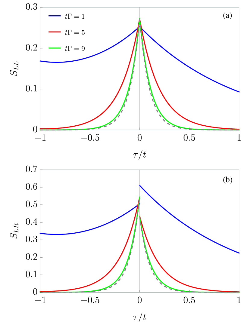
Figure 5: Comparison between auto- and cross-current correlation functions in the weak-coupling regime, $S_{\alpha\alpha^{\prime}}^{\text{ME}}(t,t+\tau)$, as a function of $\tau/t$. Since $\tau\in[-t,t]$, it is convenient to plot the functions in terms of the rescaled variable $\tau/t$ in the range $[-1,1]$. This choice allows easier comparison of the curves. Different colors indicate different values of $t\Gamma=1,5,9$. The gray dashed line represents the stationary limit $S^{\text{ME}}_{\alpha\alpha^{\prime},ss}(\tau)$. Notice the discontinuity in the cross-current correlation function at $\tau/t=0$. The other parameters are $\Gamma_{L}=1$, $\Gamma_{R}=2$, $\epsilon_{d}/\Gamma=1$, $\mu_{L}=-\mu_{R}=\Gamma/2$ and $T_{L}=T_{R}=\Gamma/100$ ($\hbar,k_{B}=1$).

VI Connecting the different frameworks

In Sec. III, we have used the HE approach to derive the exact expressions for the particle and energy currents for a single-level QD in a two-terminal setup, as well as the auto- and cross-current correlation functions. Moreover, we have benchmarked the steady-state with the LB framework by taking the limit $t\to\infty$ of the exact solution. Moving forward to Section V, we reproduced these expressions within a Master Equation (ME) framework. However, we have yet to address the crucial aspect of how the ME results can be derived from the HE and LB approaches by appropriate limiting procedures. This step is essential for a comprehensive understanding and completion of the overarching framework depicted in Fig. 1. To pursue this, a weak-coupling limit must be considered to obtain meaningful results within the framework of ME. However, achieving this limit is generally not a straightforward task, see for instance Ref. [78] discussing regularization procedures in the transient regime. While it might appear intuitive to take $\Gamma_{L},\Gamma_{R}\rightarrow 0$ as the weak-coupling limit, this is not correct. A simple argument elucidates this point: currents in the HE approach are proportional to the coupling rates, as evident in Eqs. (64) and (65). Adopting this naive limit would invariably yield zero currents, essentially signifying a quantum dot completely decoupled from its reservoirs. A similar argument holds for the current correlation function. This simple reasoning shows the necessity of a specific protocol to connect the three approaches. In the following, we discuss the steps to implement such a protocol and apply it to the currents and current correlations.

VI.1 Weak-coupling protocol

There are two key aspects of the procedure to obtain ME results from HE approach.

1) The first crucial element is the limit of small system-reservoir coupling $\Gamma$, which is a fundamental characteristic of the ME approach. In this respect, it is important to note that while the particle and energy currents are of the order $\mathcal{O}\left(\Gamma\right)$, the current correlation function is of the order $\mathcal{O}\left(\Gamma^{2}\right)$. Consequently, as mentioned above, directly taking the limit as $\Gamma\to 0$ would yield zero values for both currents and current correlation. To address this issue, we adopt a remedial approach. We first divide the respective expressions by $\Gamma$ and $\Gamma^{2}$, then take the limit $\Gamma\to 0$, and finally, multiply the obtained expressions by $\Gamma$ and $\Gamma^{2}$ again, giving us the contribution which is lowest order in the couplings.
2) The second aspect concerns the time precision, $\Gamma^{-1}$, of any Markovian master equation, which is set by the system-reservoir coupling strength. Therefore, the transient description of the dynamics from the master equation is reliable only if the time interval $t-t_{0}$ is large enough to compensate for the small value of $\Gamma$. As a result, when taking the $\Gamma\to 0$ limit, it is crucial to treat the quantity $\Gamma\left(t-t_{0}\right)$ as a constant. Mathematically, the weak-coupling protocol can be expressed in the following form,

$$I_{\alpha}^{\text{ME}}(t) =\Gamma\lim_{\Gamma\to 0}\frac{I_{\alpha}^{\text{HE}}(t)}{\Gamma}$$ (100)

$$J_{\alpha}^{\text{ME}}(t) =\Gamma\lim_{\Gamma\to 0}\frac{J_{\alpha}^{\text{HE}}(t)}{\Gamma}$$ (101)

$$S_{\alpha\alpha^{\prime}}^{\text{ME}}(t,t^{\prime}) =\Gamma^{2}\lim_{\Gamma\to 0}\frac{S_{\alpha\alpha^{\prime}}^{\text{HE}}(t,t^{\prime})}{\Gamma^{2}},$$ (102)

with $\Gamma(t-t_{0})$ kept constant. This is illustrated in Fig. 1, panels (a) to (b). We refer to the combined application of these steps as the weak-coupling protocol of the exact solution. This approach allows us to properly obtain the desired ME results from the HE results.

VI.2 Weak-coupling limit of currents

We now explain how the above weak-coupling protocol can be applied to the particle and energy currents in the single-level QD model. As explained above, we begin by dividing the exact current solutions given in Eqs. (64) and (65) by $\Gamma$, and then take the limit as $\Gamma\to 0$. This limit corresponds to taking the limit of the functions presented in Eqs. (66)-(68),

$$\lim_{\Gamma\to 0}A_{\gamma}^{m} =\epsilon_{d}^{m}f_{\gamma}(\epsilon_{d})$$ (103)

$$\lim_{\Gamma\to 0}B_{\gamma}^{m} =\epsilon_{d}^{m}e^{-\frac{\Gamma(t-t_{0})}{2}}f_{\gamma}(\epsilon_{d})$$ (104)

$$\lim_{\Gamma\to 0}C_{\gamma}^{m} =\frac{\epsilon_{d}^{m}e^{-\frac{\Gamma(t-t_{0})}{2}}}{2}f_{\gamma}(\epsilon_{d})$$ (105)

To compute the above expressions, we have performed a change of variable $\epsilon\to\Gamma\epsilon$, which enables us to extract the Fermi-Dirac function evaluated at the energy of the dot outside the integral. Crucially, while taking the limit, we kept the factor $\Gamma(t-t_{0})$ constant, respecting the temporal-resolution of ME dynamics.

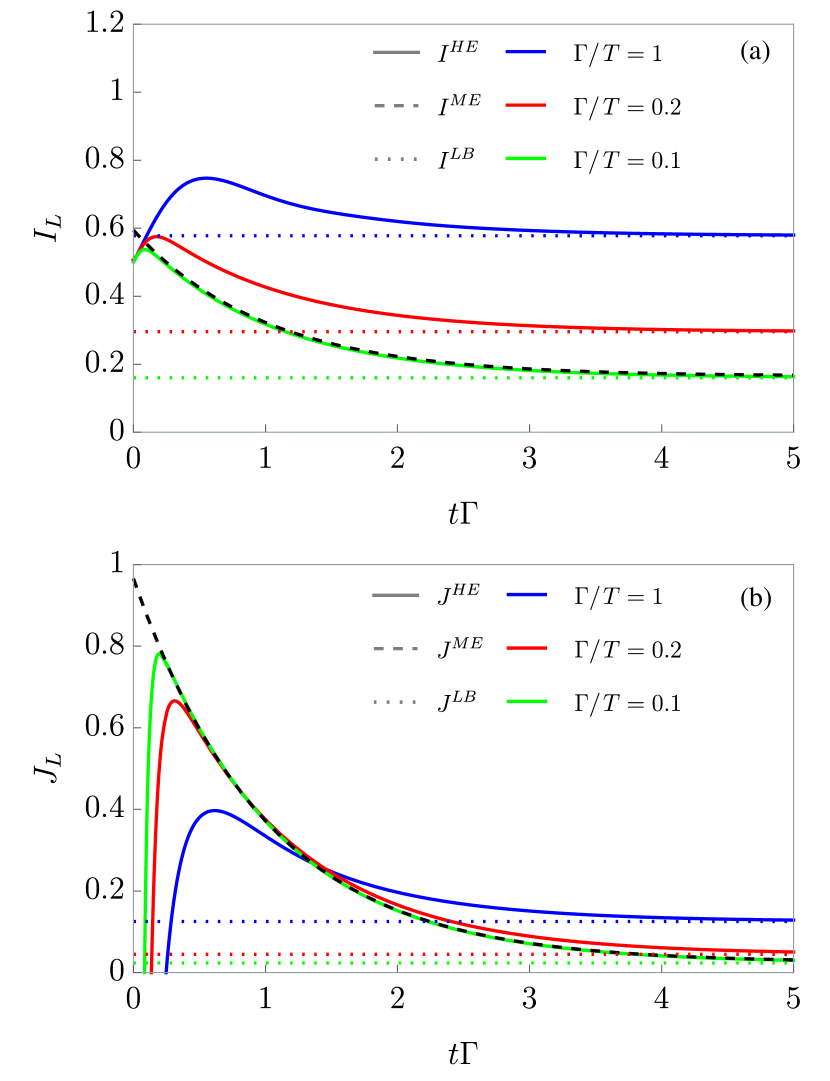
Figure 6: (a) Particle current and (b) energy current as a function of $t\Gamma$, for different values of $\Gamma/T=1,0.2,0.1$. Solid curves correspond to the result obtained with the HE (i.e., the exact solution), dashed black curves correspond to ME (i.e., the weak-coupling limit), calculated with $\Gamma/T=0.1$, and dotted lines to the LB (i.e., the stationary limit). The ME and HE results agree with each other for the weak-coupling case $\Gamma/T=0.1$. The other parameters are $\Gamma_{L}=\Gamma_{R}=1$ and $\mu_{L}=-\mu_{R}=\Gamma/2$ ($h,k_{B}=1$).

Furthermore, we employed the following exact expressions,

$$\int\frac{d\epsilon}{2\pi}\frac{1}{\frac{1}{4}+\epsilon^{2}}=1,$$ (106)

$$\int\frac{d\epsilon}{2\pi}\frac{\cos(\epsilon\Gamma t)}{\frac{1}{4}+\epsilon^{2}}=e^{-\Gamma t/2},$$ (107)

$$\int\frac{d\epsilon}{2\pi}\frac{\epsilon\sin(\epsilon\Gamma t)}{\frac{1}{4}+\epsilon^{2}}=\frac{e^{-\Gamma t/2}}{2}.$$ (108)

By substituting the above expressions into Eqs. (64) and (65), and multiplying again by $\Gamma$, we exactly recover the same results obtained with the ME approach given in Eqs. (91) and (92). As a technical remark, it is important to stress that our weak-coupling limit procedure leads to the correct ME results, which otherwise cannot be obtained by simply considering the Lorentzian under the integrals of Eqs. (66)-(68) to become a Dirac delta in the limit of small $\Gamma$.

In Fig. 6 we show (a) the particle and (b) energy currents as functions of $t\Gamma$, for different values of $\Gamma/T$ and for all three approaches. For both currents, in the weak-coupling regime, i.e., for small values of $\Gamma/T$ (green curves), the currents obtained with the HE coincide with those obtained using the ME (i.e., solid green curves overlap with the dashed black ones). In general, the ME results are not expected to agree with the LB ones in the stationary limit (for $t\Gamma\gg 1$, which violates the weak-coupling assumption). However, in the weak-coupling regime (when $\Gamma/T\ll 1$), the steady state of the ME result matches the LB result exactly. On the other hand, the HE approach always reproduces the correct stationary solution.

Moreover, Fig. 6 demonstrates that although the currents are well described in the WBL at intermediate and long time, there are peculiarities at short times. Specifically, we see that the particle current exhibits a jump at short times. On the other hand, the energy current shows a divergence at small time. This pathological behavior of the currents can be understood intuitively by noting that short times implies a wide spread in energy [55], which invalidates the use of the WBL. A possible way to solve this problem can be to consider an energy-dependent tunneling rate function $\Gamma(\epsilon)$ with an energy cut-off or decay. Possible choices include Lorentzian- and a boxcar-shaped function [34].

VI.3 Weak-coupling limit of the current correlation function

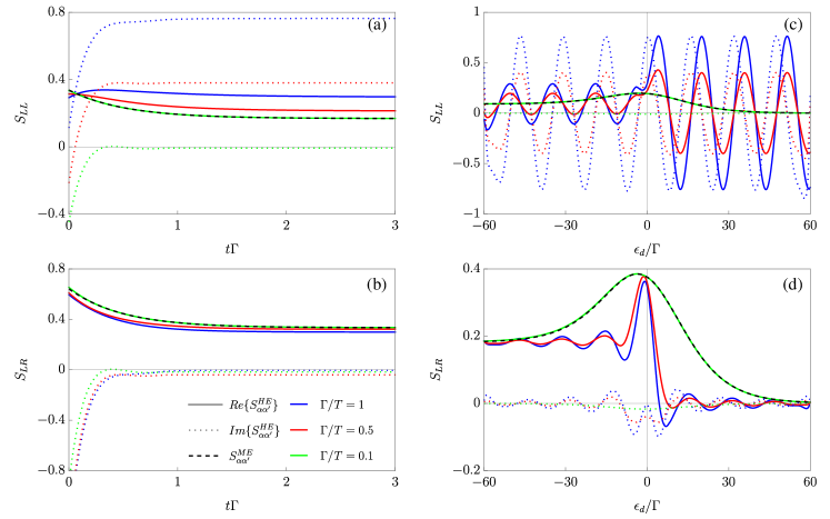
Figure 7: Auto- ($S_{LL}$) and cross- ($S_{LR}$) current correlations as functions of time $t\Gamma$ (at fixed $\epsilon_{d}/\Gamma=1$, left panels, (a) and (b)) and as functions of the energy of the dot $\epsilon_{d}/\Gamma$ (at fixed $t\Gamma=1$, right panels, (c) and (d)). Similar results hold for $S_{RR}$ and $S_{RL}$. Solid curves correspond to $\text{Re}\{S_{\alpha\alpha^{\prime}}^{HE}\}$ and dotted curves correspond to $\text{Im}\{S_{\alpha\alpha^{\prime}}^{HE}\}$ obtained with the HE approach, the dashed curves represents the ME result (obtained with $\Gamma/T=0.1$). Different colors indicate different values of $\Gamma/T=1,0.5,0.1$. The other parameters are $\Gamma_{L}=\Gamma_{R}=1$ and $\mu_{L}=-\mu_{R}=\Gamma/2$, $\tau\Gamma=0.4$.

We now explain how the expression for the current correlation function of Eq. (97) obtained with the ME approach can be computed starting from the exact solution of Eq. (IV.1), obtained within the HE picture, by taking the weak-coupling limit. To this end, using the same weak-coupling procedure as for the currents, we take first the limit of $S_{\alpha\alpha^{\prime}}^{\text{HE}}(t,t^{\prime})/\Gamma^{2}$ as $\Gamma\to 0$. This is equivalent to taking the limit for small coupling of the Lambda functions defined in Eqs. (70),

$$\lim_{\Gamma\to 0}\Lambda_{0}(t,t^{\prime}) =\frac{e^{i\epsilon_{d}(t-t^{\prime})}}{2}e^{-\frac{\Gamma}{2}(t+t^{\prime})}e^{\Gamma t_{0}}n_{d}$$ (109)

$$\lim_{\Gamma\to 0}\Lambda^{-}_{\gamma}(t,t^{\prime}) =e^{i\epsilon_{d}(t-t^{\prime})}\left[\Theta(t^{\prime}-t)e^{-\frac{\Gamma}{2}\absolutevalue{t-t^{\prime}}}-\Theta(t_{0}-t)e^{-\frac{\Gamma}{2}(t^{\prime}-t_{0})}e^{-\frac{\Gamma}{2}\absolutevalue{t-t_{0}}}\right]f_{\gamma}(\epsilon_{d})$$

$$\lim_{\Gamma\to 0}\Lambda^{\pm}_{\gamma}(t,t^{\prime}) =\frac{e^{i\epsilon_{d}(t-t^{\prime})}}{2}\left[e^{-\frac{\Gamma}{2}\absolutevalue{t-t^{\prime}}}+e^{-\frac{\Gamma}{2}(t+t^{\prime})}e^{\Gamma t_{0}}-e^{-\frac{\Gamma}{2}(t^{\prime}-t_{0})}e^{-\frac{\Gamma}{2}\absolutevalue{t-t_{0}}}-e^{-\frac{\Gamma}{2}(t-t_{0})}e^{-\frac{\Gamma}{2}\absolutevalue{t^{\prime}-t_{0}}}\right]f_{\gamma}(\epsilon_{d}),$$

$$\lim_{\Gamma\to 0}\Lambda_{\gamma}(t,t^{\prime}) =\frac{2e^{i\epsilon_{d}(t-t^{\prime})}}{\Gamma}f_{\gamma}(\epsilon_{d})\delta(t-t^{\prime})$$

By substituting the above expressions back into Eq. (IV.1), it is possible to show analytically that the two approaches lead to the same result.

In Fig. 7 we show the auto- and cross-current fluctuations as functions of time and as functions of the energy of the dot. As can be clearly seen, the result obtained with the HE approaches the one obtained with the ME approach in the limit of weak coupling, namely for small values of $\Gamma/T$ (green curves). We emphasize that the ME current correlation function is a real quantity as seen from Eq. (97). This is further illustrated in Fig. 7 where, for small coupling, the real part of the exact HE result converges to the ME one (black dashed curve), while the imaginary part vanishes. However, as the coupling strength increases, the ME result deviates from the HE one (red and blue curves), emphasizing that the ME result remains valid only under weak-coupling conditions.
In panels (c) and (d), we look at the current correlation as a function of the energy of the dot. In this case, the behavior between the two results, from the HE and ME approaches, is completely different. In particular, the ME approach fails to display the periodic oscillations which are present in the strong coupling regime using the exact HE approach. These oscillations arise from quantum coherent effects as we have already discussed in the case of the currents in Fig. 4.

As a final result, we illustrate the connection between shot noise in the LB framework and the ME result. To achieve this, we must compute the integral with respect to $\tau$ from Eq. (V.4). This corresponds to the Fourier transform at the frequency $\omega=0$,

$$\int d\tau S^{\text{ME}}_{\alpha\alpha^{\prime},ss}(\tau) =\pm\frac{\Gamma_{L}\Gamma_{R}}{\Gamma}\left[f_{L}\left(1-f_{R}\right)+f_{R}\left(1-f_{L}\right)\right]$$

$$\mp 2\frac{\Gamma_{L}^{2}\Gamma_{R}^{2}}{\Gamma^{3}}\left(f_{L}-f_{R}\right)^{2},$$ (110)

where $\pm$ distinguishes between auto- ($\alpha=\alpha^{\prime}$) and cross-current ($\alpha\neq\alpha^{\prime}$) correlations. It is straightforward to show that, by following the weak-coupling protocol discussed previously in this section, the above result coincides with the LB shot noise for small $\Gamma$, i.e., $\Gamma^{2}\left(\lim_{\Gamma\to 0}S_{\alpha\alpha^{\prime}}^{\text{LB}}(\omega=0)/\Gamma^{2}\right)$.

VII Conclusions

In this work, we have employed three distinct frameworks — Heisenberg equations, master equations, and Landauer-Büttiker — for the computation of currents and current correlation in open quantum systems. While the HE and LB frameworks inherently encapsulate the natural definitions of current and correlations, the ME framework poses notable challenges. To address them, we introduced a general approach to Full Counting Statistics capturing transient dynamics involving multiple times, multiple reservoirs and non-instantaneous jumps.

Using the paradigmatic example of a single-level quantum dot coupled to two fermionic reservoirs, we bridged HE and ME through a rigorously designed weak-coupling protocol. This not only allowed us to make a connection between the two frameworks but also laid bare some critical aspects and shortcomings of master equations that are often overlooked, such as the temporal resolution of transient dynamics. Furthermore, we benchmarked both approaches in the steady state against the results obtained from the LB formalism. Overall, our analysis not only validated the consistency of our theoretical framework but also shed light on the interplay between the different approaches, providing a comprehensive understanding of their respective strengths and limitations.

While we expect our generalized FCS procedure to be an important addition to the ME toolbox, the utility of our HE results also goes beyond the example of a single quantum dot discussed in this article. The calculation of currents and current correlations are crucial for topics such as fluctuation-dissipation relations [12, 13], thermodynamic uncertainty relations [14, 15, 16, 17] and quantum metrology [18, 19, 20], which are important problems in open quantum systems, as well as for modeling experiments in these directions.

We believe that this work will serve as a comprehensive resource for researchers in the field of open quantum systems, especially for those seeking guidance when utilizing multiple techniques or when delving into less familiar methodologies to address specific problems.

Appendix A Multi-time multi-terminal joint probability with GFCS

In this section, we derive the multi-time expression for the joint probability $P^{>}\left(\vec{x}^{(1)},t_{1};\vec{x}^{(2)},t_{2};\ldots;\vec{x}^{(N)},t_{N}\right)$, defined as the probability of having a net amount of $\vec{x}^{(1)}$ quanta transferred within time $t_{1}-t_{0}$, $\vec{x}^{(2)}$ within time $t_{2}-t_{0}$, and so on. Eq. (II.2.1) of the main text corresponds to the case of $N=2$. The full joint probability distribution can be derived from the marginal probability $P\left(\vec{x}_{N};t_{N}\right)$. Using the Chapman–Kolmogorov property for Markovian evolution, the marginal probability can be expressed in the following form,

$$P\left(\vec{x}_{N};t_{N}\right)=\sum_{\vec{x}_{1},\ldots,\vec{x}_{N-1}}\Tr{\Omega\left(\vec{x}^{(N)}-\vec{x}^{(N-1)};s_{N}-s_{N-1}\right)\Omega\left(\vec{x}^{(N-1)}-\vec{x}^{(N-2)};s_{N-1}-s_{N-2}\right)\ldots\Omega\left(\vec{x}^{(1)};s_{1}\right)\rho_{0}}.$$ (111)

This corresponds to Eq. (25) in Ref. [45], generalized to the case of multi-terminals, and for any quanta $\vec{x}$ of particles, charges, or energies exchanged between the system and the reservoirs. Then, since we have $P\left(n_{N};t_{N}\right)=\sum_{n_{1},\ldots,n_{N-1}}P^{>}\left(n_{1},t_{1},\ldots,n_{N},t_{N}\right)$, by direct inspection, we find,

$$P^{>}\left(\vec{x}^{(1)},t_{1};\vec{x}^{(2)},t_{2};\ldots;\vec{x}^{(N)},t_{N}\right)=\Tr{\left[\prod_{k=1}^{N}\Omega\left(\vec{x}^{(N-k+1)}-\vec{x}^{(N-k)};s_{N-k+1}-s_{N-k}\right)\right]\rho_{0}},$$ (112)

which in the $\vec{\chi}$-space takes the following form,

$$P^{>}\left(\vec{\chi}^{(1)},t_{1};\vec{\chi}^{(2)},t_{2};\ldots;\vec{\chi}^{(N)},t_{N}\right)=\Tr{\left[\prod_{k=1}^{N}\Omega\left(\sum_{i=N}^{N-k+1}\vec{\chi}^{(i)};s_{N-k+1}-s_{N-k}\right)\right]\rho_{0}}.$$ (113)

The above result may be alternatively derived using Bayes’ theorem for the conditional density operator and using Von Neumann’s projection postulate, as presented in Refs. [44, 45].

Appendix B Calculation of observables with GFCS

In this section, we show how to compute expectation values of observables using the GFCS method introduced in Sec. II.2.1. First, we consider the average number of tunneled particles, charges, or energy quanta exchanged with reservoir $\alpha$ within time $t^{\prime}-t_{0}$. Using the marginal property of the joint probability distribution, it takes the following form,

$$\expectationvalue{x^{\prime}_{\alpha}(t^{\prime})}_{\text{ME}} =\int_{t_{0}}^{t^{\prime}}ds^{\prime}F(t^{\prime}-s^{\prime})\sum_{\vec{x}^{\prime}}x^{\prime}_{\alpha}P({\vec{x}}^{\prime},s^{\prime})=\int_{t_{0}}^{t^{\prime}}ds^{\prime}F(t^{\prime}-s^{\prime})\sum_{\vec{x}\vec{x}^{\prime}}x^{\prime}_{\alpha}P^{>}(\vec{x},s;\vec{x}^{\prime},s^{\prime})$$

$$=\int_{t_{0}}^{t^{\prime}}ds^{\prime}F(t^{\prime}-s^{\prime})\partial_{i\chi^{\prime}_{\alpha}}\sum_{\vec{x}\vec{x}^{\prime}}P^{>}(\vec{x},s;\vec{x}^{\prime},s^{\prime})e^{i\vec{x}\cdot\vec{\chi}}e^{i\vec{x}^{\prime}\cdot\vec{\chi}^{\prime}}\big{\rvert}_{\vec{\chi},\vec{\chi}^{\prime}=0}$$

$$=\int_{t_{0}}^{t^{\prime}}ds^{\prime}F(t^{\prime}-s^{\prime})\partial_{i\chi^{\prime}_{\alpha}}P^{>}(\vec{\chi},s;\vec{\chi}^{\prime},s^{\prime})\big{\rvert}_{\vec{\chi},\vec{\chi}^{\prime}=0},$$ (114)

where we have introduced the detection response function $F$, and the joint probability in the $\vec{\chi}$-space,

$$P^{>}(\vec{\chi},s;\vec{\chi}^{\prime},s^{\prime}) =\sum_{\vec{x}\vec{x}^{\prime}}P^{>}(\vec{x},s;\vec{x}^{\prime},s^{\prime})e^{i\vec{x}\cdot\vec{\chi}}e^{i\vec{x}^{\prime}\cdot\vec{\chi}^{\prime}}$$

$$=\Tr{\Omega(\vec{\chi}^{\prime},t^{\prime}-t)\Omega(\vec{\chi}+\vec{\chi}^{\prime},t-t_{0})\rho_{0}}$$

$$=\Tr{e^{\mathcal{L}(\vec{\chi}^{\prime})(t^{\prime}-t)}e^{\mathcal{L}(\vec{\chi}+\vec{\chi}^{\prime})(t-t_{0})}\rho_{0}}.$$ (115)

In the last line we have rewritten the propagator, $\Omega(\vec{\chi},t)=e^{\mathcal{L}(\vec{\chi})t}$.

Currents with GFCS

The current associated to the counting variable $x_{\alpha}$ can be obtained taking the time derivative of Eq. (B),

$$\partial_{t^{\prime}}\expectationvalue{x_{\alpha}(t^{\prime})}_{\text{ME}} =\int_{t_{0}}^{t^{\prime}}ds^{\prime}F(t^{\prime}-s^{\prime})\partial_{i\chi^{\prime}_{\alpha}}\partial_{s^{\prime}}P^{>}(\vec{\chi},s;\vec{\chi}^{\prime},s^{\prime})\big{\rvert}_{\vec{\chi},\vec{\chi}^{\prime}=0}$$

$$=\int_{t_{0}}^{t}ds^{\prime}\,F\left(t^{\prime}-s^{\prime}\right)\partial_{i\chi^{\prime}_{\alpha}}\partial_{s^{\prime}}\Tr{e^{\mathcal{L}(\vec{\chi}^{\prime})\left(s^{\prime}-t_{0}\right)}\rho_{0}}\big{\rvert}_{\vec{\chi}^{\prime}=0}$$

$$=\int_{t_{0}}^{t}ds^{\prime}\,F\left(t-s^{\prime}\right)\Tr{\partial_{i\chi^{\prime}_{\alpha}}\mathcal{L}(\vec{\chi}^{\prime})\rvert_{\vec{\chi}^{\prime}=0}e^{\mathcal{L}\left(s^{\prime}-t_{0}\right)}\rho_{0}}.$$ (116)

Here in the first line, we used the property of the derivative of the convolution and the boundary conditions of the detection response function, $F(0)=F(t-t_{0})=0$, while in the third line we have used the trace preserving property of the Lindbladian $\Tr{\mathcal{L}(0)\sigma}=0$ (valid for any density matrix $\sigma$). In the last line, we recognize the generalized current superoperator at reservoir $\alpha$,

$$\partial_{i\chi_{\alpha}}\mathcal{L}(\vec{\chi})\big{\rvert}_{\vec{\chi}=0}=\sum_{j}\nu_{j\alpha}\left(\mathcal{L}_{j\alpha}^{+}-\mathcal{L}_{j\alpha}^{-}\right).$$ (117)

The above expression corresponds to the particle current superoperator $\mathcal{I}_{\alpha}$ for $\nu_{j\alpha}=1$, and to the energy current superoperator $\mathcal{J}_{\alpha}$ for $\nu_{j\alpha}=\epsilon_{j}$ of Eqs. (39) and (40) respectively.

Two-time current correlation with GFCS

As mentioned in Eq. (II.2.1) of the main text, the two-time current correlation can be written in the following manner,

$$\left\langle I_{\alpha}(t)I_{\alpha^{\prime}}(t^{\prime})\right\rangle_{\text{ME}} =\int_{t_{0}}^{t}ds\int_{t_{0}}^{t^{\prime}}ds^{\prime}F(t-s)F(t^{\prime}-s^{\prime})~{}\left[\partial_{i\chi_{\alpha}}\partial_{i\chi^{\prime}_{\alpha^{\prime}}}\partial_{s}\partial_{s^{\prime}}P(\vec{\chi},s;\vec{\chi}^{\prime},s^{\prime})\big{\rvert}_{\vec{\chi},\vec{\chi}^{\prime}=0}\right],$$ (118)

where we have again used the property of the derivative of the convolution and the boundary conditions of the detection response function to move the time derivatives inside the integral. Here, we recall that the time-ordered joint probability takes the following form,

$$P\left(\vec{\chi},s;\vec{\chi}^{\prime},s^{\prime}\right) =\Theta(s^{\prime}-s)P^{>}\left(\vec{\chi},s;\vec{\chi}^{\prime},s^{\prime}\right)+\Theta(s-s^{\prime})P^{<}\left(\vec{\chi},s;\vec{\chi}^{\prime},s^{\prime}\right),$$ (119)

with $P^{<}\left(\vec{\chi},s;\vec{\chi}^{\prime},s^{\prime}\right)=P^{>}\left(\vec{\chi}^{\prime},s^{\prime};\vec{\chi},s\right)$. The term in square parenthesis in Eq. (118), can be computed by performing a change of variable. In particular by substituting $\tau=s^{\prime}-s$ and $t=s$, and using the property of the derivative of the Dirac delta function $-\delta^{\prime}(\tau)f(\tau)=\delta(\tau)f^{\prime}(0)$, we can write it in the following form,

$$\partial_{i\chi_{\alpha}}\partial_{i\chi^{\prime}_{\alpha^{\prime}}}\partial_{s}\partial_{s^{\prime}}P(\vec{\chi},s;\vec{\chi}^{\prime},s^{\prime})\big{\rvert}_{\vec{\chi},\vec{\chi}^{\prime}=0} =\partial_{i\chi_{\alpha}}\partial_{i\chi_{\alpha^{\prime}}^{\prime}}\delta(\tau)\left(\partial_{t}-\partial_{\tau}\right)\left[P^{>}(\vec{\chi},t;\vec{\chi}^{\prime},t+\tau)-P^{<}(\vec{\chi},t;\vec{\chi}^{\prime},t+\tau)\right]\big{\rvert}_{\vec{\chi},\vec{\chi}^{\prime}=0}$$

$$+\partial_{i\chi_{\alpha}}\partial_{i\chi_{\alpha^{\prime}}^{\prime}}\Theta(\tau)(-\partial_{\tau}^{2}+\partial_{\tau}\partial_{t})\mathcal{P}^{>}(\vec{\chi},t;\vec{\chi}^{\prime},t+\tau)\big{\rvert}_{\vec{\chi},\vec{\chi}^{\prime}=0}$$

$$+\partial_{i\chi_{\alpha}}\partial_{i\chi_{\alpha^{\prime}}^{\prime}}\Theta(-\tau)(-\partial_{\tau}^{2}+\partial_{\tau}\partial_{t})\mathcal{P}^{<}(\vec{\chi},t;\vec{\chi}^{\prime},t+\tau)\big{\rvert}_{\vec{\chi},\vec{\chi}^{\prime}=0}$$ (120)

We can now calculate the above three terms. The first term can be simplified as,

$$\text{(i)}\rightarrow\quad \partial_{i\chi_{\alpha}}\partial_{i\chi_{\alpha^{\prime}}^{\prime}}\delta(\tau)\left(\partial_{t}-\partial_{\tau}\right)\left[P^{>}(\vec{\chi},t;\vec{\chi}^{\prime},t+\tau)-P^{<}(\vec{\chi},t;\vec{\chi}^{\prime},t+\tau)\right]\Big{\rvert}_{\vec{\chi},\vec{\chi}^{\prime}=0}$$

$$~{}~{}~{}~{}=\partial_{i\chi_{\alpha}}\partial_{i\chi_{\alpha^{\prime}}^{\prime}}\delta(\tau)\left(\partial_{t}-\partial_{\tau}\right)\Tr{e^{\mathcal{L}(\vec{\chi}^{\prime})\tau}e^{\mathcal{L}(\vec{\chi}+\vec{\chi}^{\prime})t}\rho_{0}-e^{\mathcal{-L(\vec{\chi})\tau}}e^{\mathcal{L}(\vec{\chi}+\vec{\chi}^{\prime})(t+\tau)}\rho_{0}}\Big{\rvert}_{\vec{\chi},\vec{\chi}^{\prime}=0}$$

$$~{}~{}~{}~{}=\partial_{i\chi_{\alpha}}\partial_{i\chi_{\alpha^{\prime}}^{\prime}}\delta(\tau)\Tr{\mathcal{L}(\vec{\chi}^{\prime}+\vec{\chi})\rho(\vec{\chi}^{\prime}+\vec{\chi},t)-\mathcal{L}(\vec{\chi}^{\prime})\rho(\vec{\chi}^{\prime}+\vec{\chi},t)-\mathcal{L}(\vec{\chi})\rho(\vec{\chi}^{\prime}+\vec{\chi},t)}\big{\rvert}_{\vec{\chi},\vec{\chi}^{\prime}=0}$$

$$~{}~{}~{}~{}=\delta(\tau)\Tr{\partial_{i\chi_{\alpha}}\partial_{i\chi_{\alpha^{\prime}}^{\prime}}\mathcal{L}(\vec{\chi}^{\prime}+\vec{\chi})\big{\rvert}_{\vec{\chi},\vec{\chi}^{\prime}=0}\rho(t)}$$

$$~{}~{}~{}~{}=\delta(\tau)\Tr{\partial_{i\chi_{\alpha}}\partial_{i\chi_{\alpha^{\prime}}^{\prime}}\left[\mathcal{L}_{0}+\sum_{j\beta}\left(e^{i(\chi_{\beta}+\chi^{\prime}_{\beta})\nu_{j\beta}}\mathcal{L}_{j\beta}^{+}+e^{-i(\chi_{\beta}+\chi^{\prime}_{\beta})\nu_{j\beta}}\mathcal{L}_{j\beta}^{-}\right)\right]\Big{\rvert}_{\vec{\chi},\vec{\chi}^{\prime}=0}~{}\rho(t)}$$

$$~{}~{}~{}~{}=\delta(\tau)\Tr{\partial_{i\chi_{\alpha}}\left[\sum_{j}\nu_{j\alpha^{\prime}}\left(e^{i\chi_{\alpha^{\prime}}\nu_{j\alpha^{\prime}}}\mathcal{L}_{j\alpha^{\prime}}^{+}-e^{-i\chi_{\alpha^{\prime}}\nu_{j\alpha^{\prime}}}\mathcal{L}_{j\alpha^{\prime}}^{-}\right)\right]\Huge\rvert_{\vec{\chi}\vec{=}0}~{}\rho(t)}$$

$$~{}~{}~{}~{}=\delta(\tau)\delta_{\alpha\alpha^{\prime}}\Tr{\sum_{j}\nu_{j\alpha}^{2}\left(\mathcal{L}_{j\alpha}^{+}+\mathcal{L}_{j\alpha}^{-}\right)\rho(t)}$$

$$~{}~{}~{}~{}=\delta(\tau)\delta_{\alpha\alpha^{\prime}}\Tr{\mathcal{A}_{\alpha}e^{\mathcal{L}(t-t_{0})}\rho_{0}}.$$

Here, in the third line we have used the property of the Dirac delta function, $\delta(\tau)f(\tau)=\delta(\tau)f(0)$, and the trace preserving property of the Lindbladian $\Tr{\mathcal{L}(0)\sigma}=0$ for any density matrix $\sigma$. In the fourth line, we have substituted the expression of $\mathcal{L}(\vec{\chi}^{\prime}+\vec{\chi})$ as presented in Eq. (31). Finally, in the last line, we have identified the activity, $\mathcal{A}_{\alpha}$, which counts the total number of quantum jumps in or out of the system. The second term of Eq. (B) takes the following form,

$$\text{(ii)}\rightarrow\quad \partial_{i\chi_{\alpha}}\partial_{i\chi_{\alpha^{\prime}}^{\prime}}\Theta(\tau)(-\partial_{\tau}^{2}+\partial_{\tau}\partial_{t})P^{>}(\vec{\chi},t;\vec{\chi}^{\prime},t+\tau)\big{\rvert}_{\vec{\chi},\vec{\chi}^{\prime}=0}$$

$$~{}~{}~{}~{}=\partial_{i\chi_{\alpha}}\partial_{i\chi_{\alpha^{\prime}}^{\prime}}\Theta(\tau)(-\partial_{\tau}^{2}+\partial_{\tau}\partial_{t})\Tr{e^{\mathcal{L}(\vec{\chi}^{\prime})\tau}e^{\mathcal{L}(\vec{\chi}+\vec{\chi}^{\prime})t}\rho_{0}}\big{\rvert}_{\vec{\chi},\vec{\chi}^{\prime}=0}$$

$$~{}~{}~{}~{}=\Theta(\tau)\partial_{i\chi_{\alpha}}\partial_{i\chi_{\alpha^{\prime}}^{\prime}}\Tr{\mathcal{L}(\vec{\chi}^{\prime})\left(e^{\mathcal{L}(\vec{\chi}^{\prime})\tau}\mathcal{L}(\vec{\chi}+\vec{\chi}^{\prime})-\mathcal{L}(\vec{\chi}^{\prime})e^{\mathcal{L}(\vec{\chi}^{\prime})\tau}\right)\rho(\vec{\chi}+\vec{\chi}^{\prime},t)}\big{\rvert}_{\vec{\chi},\vec{\chi}^{\prime}=0}$$

$$~{}~{}~{}~{}=\Theta(\tau)\partial_{i\chi_{\alpha}}\Tr{\left[\partial_{i\chi_{\alpha^{\prime}}^{\prime}}\mathcal{L}(\vec{\chi}^{\prime})\right]_{\vec{\chi}^{\prime}=0}\left(e^{\mathcal{L}(0)\tau}\mathcal{L}(\vec{\chi})-\mathcal{L}(0)e^{\mathcal{L}(0)\tau}\right)\rho(\vec{\chi},t)}\big{\rvert}_{\vec{\chi}=0}$$

$$~{}~{}~{}~{}=\Theta(\tau)\partial_{i\chi_{\alpha}}\Tr{\left[\partial_{i\chi_{\alpha^{\prime}}^{\prime}}\mathcal{L}(\vec{\chi}^{\prime})\right]_{\vec{\chi}^{\prime}=0}e^{\mathcal{L}(0)\tau}\left[\partial_{i\chi_{\alpha}}\mathcal{L}(\vec{\chi})\right]_{\vec{\chi}=0}\rho(t)}$$

$$~{}~{}~{}~{}=\Theta(\tau)\Tr{\mathcal{I}_{\alpha^{\prime}}e^{\mathcal{L}\tau}\mathcal{I}_{\alpha}e^{\mathcal{L}(t-t_{0})}\rho_{0}},$$

and similarly, the last term of Eq. (B) can be written as,

$$\text{(iii)}\rightarrow\quad\partial_{i\chi_{\alpha}}\partial_{i\chi_{\alpha^{\prime}}^{\prime}}\Theta(-\tau)(-\partial_{\tau}^{2}+\partial_{\tau}\partial_{t})P^{<}(\vec{\chi},t;\vec{\chi}^{\prime},t+\tau)\big{\rvert}_{\vec{\chi},\vec{\chi}^{\prime}=0}=\Theta(-\tau)\Tr{\mathcal{I}_{\alpha}e^{-\mathcal{L}\tau}\mathcal{I}_{\alpha^{\prime}}e^{\mathcal{L}(t+\tau-t_{0})}\rho_{0}}.$$

Substituting expressions (i)-(iii) in Eq. (B), and going back to the time variables $s^{\prime}=t+\tau$ and $s=t$, the two-time current correlation takes the final form given in the main text, which we rewrite here for reference,

$$\left\langle I_{\alpha}(t)I_{\alpha^{\prime}}(t^{\prime})\right\rangle_{\text{ME}} =\delta_{\alpha\alpha^{\prime}}\int_{t_{0}}^{t}ds\,F\left(t-s\right)F\left(t^{\prime}-s\right)\text{Tr}\{\mathcal{A}_{\alpha}\,e^{\mathcal{L}\left(t^{\prime}-t_{0}\right)}\rho_{0}\}$$

$$+\int_{t_{0}}^{t}ds\int_{t_{0}}^{t^{\prime}}ds^{\prime}F(t-s)F(t^{\prime}-s^{\prime})\Theta\left(s^{\prime}-s\right)\text{Tr}\{\mathcal{I}_{\alpha^{\prime}}e^{\mathcal{L}\left(s^{\prime}-s\right)}\mathcal{I}_{\alpha}e^{\mathcal{L}(s-t_{0})}\rho_{0}\}$$

$$+\int_{t_{0}}^{t}ds\int_{t_{0}}^{t^{\prime}}ds^{\prime}F(t-s)F(t^{\prime}-s^{\prime})\Theta\left(s-s^{\prime}\right)\text{Tr}\{\mathcal{I}_{\alpha}e^{\mathcal{L}\left(s-s^{\prime}\right)}\mathcal{I}_{\alpha^{\prime}}e^{\mathcal{L}(s^{\prime}-t_{0})}\rho_{0}\}.$$ (121)

Appendix C Single-level QD transmission probability for the LB approach

As discussed in Section II.3, the Landauer-Büttiker approach expresses observables in terms of the energy-dependent transmission function $\mathcal{T}(\epsilon)$ [21, 22]. In the subsequent discussion, we elucidate the methodology for computing the transmission function of a single-resonant level quantum dot. To achieve this, we model the quantum dot system as a double-well junction [73, 74, 2]. The barriers to the left and right of the junction are defined by $2\times 2$ scattering matrices $\mathcal{S}_{L}$ and $\mathcal{S}_{R}$, which govern the relationship between outgoing and incident stationary states. These scattering matrices are characterized by the reflection amplitudes $r_{i}$ and $r_{i}^{\prime}$, as well as the transmission amplitudes $t_{i}$ and $t_{i}^{\prime}$ for the left ($i=L$) and right ($i=R$) barriers, respectively. Here, we assume symmetric scattering matrices, i.e., $t_{i}=t_{i}^{\prime}$. By combining the scattering matrices, $\mathcal{S}=\mathcal{S}_{L}\circ\mathcal{S}_{R}$ [2, 79, 80], we can calculate the transmission function by squaring its off-diagonal entries as follows,

$$\mathcal{T}(\epsilon)=\absolutevalue{\mathcal{S}_{LR}}^{2}=\absolutevalue{\mathcal{S}_{RL}}^{2}=\frac{T_{L}T_{R}}{1+R_{L}R_{R}-2\sqrt{R_{L}R_{R}}\cos{\theta(\epsilon)}}$$ (122)

Here, $T_{i}=\absolutevalue{t_{i}}^{2}=\absolutevalue{t_{i}^{\prime}}^{2}$ and $R_{i}=\absolutevalue{r_{i}}^{2}=\absolutevalue{r_{i}^{\prime}}^{2}$ represent the transmission and reflection probabilities for the left ($i=L$) and right ($i=R$) barriers, respectively, such that $T_{i}+R_{i}=1$ due to unitarity. Furthermore, $\theta(\epsilon)=\arg{r_{L}^{\prime}}+\arg{r_{R}}$ denotes the phase shift accumulated during one complete round-trip between the scatterers. Under the assumption that $R_{L}$ and $R_{R}$ are approximately equal to 1, the transmission function exhibits pronounced resonances when the denominator approaches zero. This situation occurs when the round-trip phase $\theta(\epsilon_{d})$ is a multiple of $2\pi$ at the resonance energy $\epsilon=\epsilon_{d}$ (representing the energy of the quantum dot). In the vicinity of these resonance values, we can expand the cosine function, obtaining the so-called Breit-Wigner formula for the transmission function [74, 40],

$$\mathcal{T}\left(\epsilon\right)\approx\frac{T_{L}T_{R}}{\left(\frac{T_{L}+T_{R}}{2}\right)^{2}+2\left(1-\cos{\theta(\epsilon)}\right)}\approx\frac{\Gamma_{L}\Gamma_{R}}{\frac{\Gamma^{2}}{4}+(\epsilon-\epsilon_{d})^{2}}.$$ (123)

Here, we used the fact that close to the resonance $2\left(1-\cos{\theta(\epsilon)}\right)\approx\left(d\theta/d\epsilon\right)^{2}\left(\epsilon-\epsilon_{d}\right)^{2}$, and we defined $\Gamma_{L,R}=\frac{d\epsilon}{dk}T_{L,R}$. Physically, $\Gamma_{L}$ and $\Gamma_{R}$ (divided by $\hbar$) represent the rates at which an electron placed between the barriers would escape into the left and right leads, respectively. To elucidate this, we note that if we express the round-trip phase shift as $\theta\approx 2kW$, where $W$ is the effective width of the well, then $\frac{d\epsilon}{d\theta}=\frac{\hbar}{\tau}$, where $\tau=2W/v$ represents the time it takes for the electron to travel from one barrier to another and back, with $v=\frac{1}{\hbar}\frac{d\epsilon}{dk}$ being velocity of the particle. Substituting in their definition, we obtain,

$$\Gamma_{L}=\hbar\frac{T_{L}}{\tau}\quad\text{and}\quad\Gamma_{R}=\hbar\frac{T_{R}}{\tau}.$$ (124)

A fraction $T_{L}$ of the attempts on the left barrier is successful, while a fraction $T_{R}$ of the attempts on the right barrier is successful. Hence, $\Gamma_{L}/\hbar$ and $\Gamma_{R}/\hbar$ tell us the number of times per second that an electron succeeds in escaping through the left and right barriers, respectively.

The expression for the transmission function provided in Eq. (123), fully determines all transport quantities, including currents and current correlation functions, as specified in the last column of Table 1.

Appendix D Heisenberg equation for the single-level QD

In this section we provide the details of how to compute Eqs. (IV.1) and (IV.1). In order to do so, we start by first writing the formal solution of the second line of Eq. (IV) as,

$$\hat{c}_{k\alpha}^{\dagger}(t)=e^{i\epsilon_{k\alpha}(t-t_{0})}\hat{c}_{k\alpha}^{\dagger}(t_{0})+i\int_{t_{0}}^{t}ds~{}e^{i\epsilon_{k\alpha}(t-s)}t_{k\alpha}\hat{d}^{\dagger}(s).$$ (125)

By substituting the above expression into the first line of of Eq. (IV) we obtain,

$$\frac{d}{dt}\hat{d}^{\dagger} =i\epsilon_{d}\hat{d}^{\dagger}+i\sum_{k,\alpha}t_{k\alpha}^{*}e^{i\epsilon_{k\alpha}(t-t_{0})}\hat{c}_{k\alpha}^{\dagger}(t_{0})-\int_{t_{0}}^{t}ds~{}\sum_{k,\alpha}\absolutevalue{t_{k\alpha}}^{2}e^{i\epsilon_{k\alpha}(t-s)}\hat{d}^{\dagger}(s).$$ (126)

The last term in the above expression can be written in the following manner,

$$\int_{t_{0}}^{t}ds~{}\sum_{k,\alpha}\absolutevalue{t_{k\alpha}}^{2}e^{i\epsilon_{k\alpha}(t-s)}\hat{d}^{\dagger}(s) =\int_{t_{0}}^{t}ds~{}\int\frac{d\epsilon}{2\pi}~{}\overbrace{2\pi\sum_{k,\alpha}\delta(\epsilon-\epsilon_{k\alpha})\absolutevalue{t_{k\alpha}}^{2}}^{\Gamma}e^{i\epsilon(t-s)}\hat{d}^{\dagger}(s)$$

$$=\Gamma\int_{t_{0}}^{t}ds~{}\overbrace{\int\frac{d\epsilon}{2\pi}~{}e^{i\epsilon(t-s)}}^{\delta(t-s)}\hat{d}^{\dagger}(s)=\frac{\Gamma}{2}\hat{d}^{\dagger}(t)$$ (127)

where we used the property, $\int_{t_{0}}^{t}ds~{}\delta(t-s)\hat{d}^{\dagger}(s)=\hat{d}^{\dagger}(t)/2$, and the definition of the bare tunneling rate function of Eq. (7). It is important to recall that in our case, since we are considering the wide-band approximation, $\Gamma$ is a constant and can thus be taken out of the integral. Then, by using the definition of $\xi^{\dagger}(t)$ given in Eq. (63), Eq. (126) takes the following form,

$$\frac{d}{dt}\hat{d}^{\dagger}=\xi^{\dagger}(t)+\left(\epsilon_{d}-\frac{\Gamma}{2}\right)\hat{d}^{\dagger}(t),$$ (128)

which can be integrated, leading to the final expression given in Eq. (IV.1). A similar expression was used in Ref. [20].

Appendix E Single-level QD exact finite-time correlation functions

Using Eq. (11), the expression of the current correlation function takes the following form,

$$S^{\text{HE}}_{\alpha\alpha^{\prime}}(t,t^{\prime})=\expectationvalue{\hat{I}_{\alpha}(t)\hat{I}_{\alpha^{\prime}}(t^{\prime})}-\expectationvalue{\hat{I}_{\alpha}(t)}\expectationvalue{\hat{I}_{\alpha^{\prime}}(t^{\prime})}.$$ (129)

Furthermore, by inserting the Hamiltonian (1) into the current operator for a single quantum dot (10), we obtain

$$\hat{I}_{\alpha}(t) =\frac{d}{dt}\hat{N}_{\alpha}=-i\left[\hat{H},\hat{N}_{\alpha}\right]=i\sum_{k}\left[t_{k\alpha}^{*}\hat{c}_{k\alpha}^{\dagger}(t)\hat{d}(t)-t_{k\alpha}\hat{d}^{\dagger}(t)\hat{c}_{k\alpha}(t)\right].$$ (130)

Using the above expression, the first term of Eq. (129) becomes,

$$\expectationvalue{\hat{I}_{\alpha}(t)\hat{I}_{\alpha^{\prime}}(t^{\prime})} =\expectationvalue{\left[i\sum_{k}\left(t_{k\alpha}^{*}\hat{c}_{k\alpha}^{\dagger}(t)\hat{d}(t)-t_{k\alpha}\hat{d}^{\dagger}(t)\hat{c}_{k\alpha}(t)\right)\right]\left[i\sum_{k^{\prime}}\left(t_{k^{\prime}\alpha^{\prime}}^{*}\hat{c}_{k^{\prime}\alpha^{\prime}}^{\dagger}(t^{\prime})\hat{d}(t^{\prime})-t_{k^{\prime}\alpha^{\prime}}\hat{d}^{\dagger}(t^{\prime})\hat{c}_{k^{\prime}\alpha^{\prime}}(t^{\prime})\right)\right]}$$

$$=-\sum_{kk^{\prime}}\left\{t_{k\alpha}^{*}t_{k^{\prime}\alpha^{\prime}}^{*}\expectationvalue{\hat{c}_{k\alpha}^{\dagger}(t)\hat{d}(t)\hat{c}_{k^{\prime}\alpha^{\prime}}^{\dagger}(t^{\prime})\hat{d}(t^{\prime})}-t_{k\alpha}^{*}t_{k^{\prime}\alpha^{\prime}}\expectationvalue{\hat{c}_{k\alpha}^{\dagger}(t)\hat{d}(t)\hat{d}^{\dagger}(t^{\prime})\hat{c}_{k^{\prime}\alpha^{\prime}}(t^{\prime})}\right.$$

$$\left.~{}~{}~{}-t_{k\alpha}t_{k^{\prime}\alpha^{\prime}}^{*}\expectationvalue{\hat{d}^{\dagger}(t)\hat{c}_{k\alpha}(t)(t)\hat{c}_{k^{\prime}\alpha^{\prime}}^{\dagger}(t^{\prime})\hat{d}(t^{\prime})}+t_{k\alpha}t_{k^{\prime}\alpha^{\prime}}\expectationvalue{\hat{d}^{\dagger}(t)\hat{c}_{k\alpha}(t)\hat{d}^{\dagger}(t^{\prime})\hat{c}_{k^{\prime}\alpha^{\prime}}(t^{\prime})}\right\}.$$ (131)

Now, using Wick’s theorem, we can decompose the four-operator expectation values into the sum of products of two-operator expectation values by performing contractions,

$$\expectationvalue{\hat{c}_{k\alpha}^{\dagger}(t)\hat{d}(t)\hat{c}_{k^{\prime}\alpha^{\prime}}^{\dagger}(t^{\prime})\hat{d}(t^{\prime})} =\expectationvalue{\hat{c}_{k\alpha}^{\dagger}(t)\hat{d}(t)}\expectationvalue{\hat{c}_{k^{\prime}\alpha^{\prime}}^{\dagger}(t^{\prime})\hat{d}(t^{\prime})}+\expectationvalue{\hat{c}_{k\alpha}^{\dagger}(t)\hat{d}(t^{\prime})}\expectationvalue{\hat{d}(t)\hat{c}_{k^{\prime}\alpha^{\prime}}^{\dagger}(t^{\prime})}$$

$$\expectationvalue{\hat{c}_{k\alpha}^{\dagger}(t)\hat{d}(t)\hat{d}^{\dagger}(t^{\prime})\hat{c}_{k^{\prime}\alpha^{\prime}}(t^{\prime})} =\expectationvalue{\hat{c}_{k\alpha}^{\dagger}(t)\hat{d}(t)}\expectationvalue{\hat{d}^{\dagger}(t^{\prime})\hat{c}_{k^{\prime}\alpha^{\prime}}(t^{\prime})}+\expectationvalue{\hat{c}_{k\alpha}^{\dagger}(t)\hat{c}_{k^{\prime}\alpha^{\prime}}(t^{\prime})}\expectationvalue{\hat{d}(t)\hat{d}^{\dagger}(t^{\prime})}$$

$$\expectationvalue{\hat{d}^{\dagger}(t)\hat{c}_{k\alpha}(t)(t)\hat{c}_{k^{\prime}\alpha^{\prime}}^{\dagger}(t^{\prime})\hat{d}(t^{\prime})} =\expectationvalue{\hat{d}^{\dagger}(t)\hat{c}_{k\alpha}(t)}\expectationvalue{\hat{c}_{k^{\prime}\alpha^{\prime}}^{\dagger}(t^{\prime})\hat{d}(t^{\prime})}+\expectationvalue{\hat{d}^{\dagger}(t)\hat{d}(t^{\prime})}\expectationvalue{\hat{c}_{k\alpha}(t)\hat{c}_{k^{\prime}\alpha^{\prime}}^{\dagger}(t^{\prime})}$$

$$\expectationvalue{\hat{d}^{\dagger}(t)\hat{c}_{k\alpha}(t)\hat{d}^{\dagger}(t^{\prime})\hat{c}_{k^{\prime}\alpha^{\prime}}(t^{\prime})} =\expectationvalue{\hat{d}^{\dagger}(t)\hat{c}_{k\alpha}(t)}\expectationvalue{\hat{d}^{\dagger}(t^{\prime})\hat{c}_{k^{\prime}\alpha^{\prime}}(t^{\prime})}+\expectationvalue{\hat{d}^{\dagger}(t)\hat{c}_{k^{\prime}\alpha^{\prime}}(t^{\prime})}\expectationvalue{\hat{c}_{k\alpha}(t)\hat{d}^{\dagger}(t^{\prime})}.$$ (132)

The calculation yields

$$\expectationvalue{I_{\alpha}(t)I_{\alpha^{\prime}}(t^{\prime})}=-\sum_{kk^{\prime}} \left\{t_{k\alpha}^{*}t_{k^{\prime}\alpha^{\prime}}^{*}\left[\expectationvalue{\hat{c}_{k\alpha}^{\dagger}(t)\hat{d}(t)}\expectationvalue{\hat{c}_{k^{\prime}\alpha^{\prime}}^{\dagger}(t^{\prime})\hat{d}(t^{\prime})}+\expectationvalue{\hat{c}_{k\alpha}^{\dagger}(t)\hat{d}(t^{\prime})}\expectationvalue{\hat{d}(t)\hat{c}_{k^{\prime}\alpha^{\prime}}^{\dagger}(t^{\prime})}\right]\right.$$

$$- \left.t_{k\alpha}^{*}t_{k^{\prime}\alpha^{\prime}}\left[\expectationvalue{\hat{c}_{k\alpha}^{\dagger}(t)\hat{d}(t)}\expectationvalue{\hat{d}^{\dagger}(t^{\prime})\hat{c}_{k^{\prime}\alpha^{\prime}}(t^{\prime})}+\expectationvalue{\hat{c}_{k\alpha}^{\dagger}(t)\hat{c}_{k^{\prime}\alpha^{\prime}}(t^{\prime})}\expectationvalue{\hat{d}(t)\hat{d}^{\dagger}(t^{\prime})}\right]\right.$$

$$- \left.t_{k\alpha}t_{k^{\prime}\alpha^{\prime}}^{*}\left[\expectationvalue{\hat{d}^{\dagger}(t)\hat{c}_{k\alpha}(t)}\expectationvalue{\hat{c}_{k^{\prime}\alpha^{\prime}}^{\dagger}(t^{\prime})\hat{d}(t^{\prime})}+\expectationvalue{\hat{d}^{\dagger}(t)\hat{d}(t^{\prime})}\expectationvalue{\hat{c}_{k\alpha}(t)\hat{c}_{k^{\prime}\alpha^{\prime}}^{\dagger}(t^{\prime})}\right]\right.$$

$$+ \left.t_{k\alpha}t_{k^{\prime}\alpha^{\prime}}\left[\expectationvalue{\hat{d}^{\dagger}(t)\hat{c}_{k\alpha}(t)}\expectationvalue{\hat{d}^{\dagger}(t^{\prime})\hat{c}_{k^{\prime}\alpha^{\prime}}(t^{\prime})}+\expectationvalue{\hat{d}^{\dagger}(t)\hat{c}_{k^{\prime}\alpha^{\prime}}(t^{\prime})}\expectationvalue{\hat{c}_{k\alpha}(t)\hat{d}^{\dagger}(t^{\prime})}\right]\right\}.$$ (133)

Putting together the first terms of all lines of the above expression, we find the product of the current expectation values. This cancels the corresponding term in the expression (129). Finally, the current correlation function takes the form given in Eq. (IV), which we rewrite for reference,

$$S^{\text{HE}}_{\alpha\alpha^{\prime}}(t,t^{\prime})=-\sum_{kk^{\prime}} \left\{t_{k\alpha}^{*}t_{k^{\prime}\alpha^{\prime}}^{*}\expectationvalue{\hat{c}_{k\alpha}^{\dagger}(t)\hat{d}(t^{\prime})}\expectationvalue{\hat{d}(t)\hat{c}_{k^{\prime}\alpha^{\prime}}^{\dagger}(t^{\prime})}-t_{k\alpha}^{*}t_{k^{\prime}\alpha^{\prime}}\expectationvalue{\hat{c}_{k\alpha}^{\dagger}(t)\hat{c}_{k^{\prime}\alpha^{\prime}}(t^{\prime})}\expectationvalue{\hat{d}(t)\hat{d}^{\dagger}(t^{\prime})}\right.$$

$$-\left.t_{k\alpha}t_{k^{\prime}\alpha^{\prime}}^{*}\expectationvalue{\hat{d}^{\dagger}(t)\hat{d}(t^{\prime})}\expectationvalue{\hat{c}_{k\alpha}(t)\hat{c}_{k^{\prime}\alpha^{\prime}}^{\dagger}(t^{\prime})}+t_{k\alpha}t_{k^{\prime}\alpha^{\prime}}\expectationvalue{\hat{d}^{\dagger}(t)\hat{c}_{k^{\prime}\alpha^{\prime}}(t^{\prime})}\expectationvalue{\hat{c}_{k\alpha}(t)\hat{d}^{\dagger}(t^{\prime})}\right\}.$$ (134)

It is convenient to rewrite the previous expression as follows,

$$S^{\text{HE}}_{\alpha\alpha^{\prime}}(t,t^{\prime})= -CD_{\alpha}(t,t^{\prime})\overline{DC}_{\alpha^{\prime}}(t,t^{\prime})+CC_{\alpha\alpha^{\prime}}(t,t^{\prime})\overline{DD}(t,t^{\prime})+\overline{CC}_{\alpha\alpha^{\prime}}(t,t^{\prime})DD(t,t^{\prime})-\overline{CD}_{\alpha}(t,t^{\prime})DC_{\alpha^{\prime}}.(t,t^{\prime})$$ (135)

where we have defined,

$$CD_{\alpha}(t,t^{\prime}) =\sum_{k}t_{k\alpha}^{*}\expectationvalue{\hat{c}_{k\alpha}^{\dagger}(t)\hat{d}(t^{\prime})} \overline{CD}_{\alpha}(t,t^{\prime}) =\sum_{k}t_{k\alpha}\expectationvalue{\hat{c}_{k\alpha}(t)\hat{d}^{\dagger}(t^{\prime})}$$

$$DC_{\alpha^{\prime}}(t,t^{\prime}) =\sum_{k^{\prime}}t_{k^{\prime}\alpha^{\prime}}\expectationvalue{\hat{d}^{\dagger}(t)\hat{c}_{k^{\prime}\alpha^{\prime}}(t^{\prime})} \overline{DC}_{\alpha^{\prime}}(t,t^{\prime}) =\sum_{k^{\prime}}t_{k^{\prime}\alpha^{\prime}}^{*}\expectationvalue{\hat{d}(t)\hat{c}_{k^{\prime}\alpha^{\prime}}^{\dagger}(t^{\prime})}$$

$$CC_{\alpha\alpha^{\prime}}(t,t^{\prime}) =\sum_{kk^{\prime}}t_{k\alpha}^{*}t_{k^{\prime}\alpha^{\prime}}\expectationvalue{\hat{c}_{k\alpha}^{\dagger}(t)\hat{c}_{k^{\prime}\alpha^{\prime}}(t^{\prime})} \overline{CC}_{\alpha\alpha^{\prime}}(t,t^{\prime}) =\sum_{kk^{\prime}}t_{k\alpha}t^{*}_{k^{\prime}\alpha^{\prime}}\expectationvalue{\hat{c}_{k\alpha}(t)c^{\dagger}_{k^{\prime}\alpha^{\prime}}(t^{\prime})}$$

$$DD(t,t^{\prime}) =\expectationvalue{\hat{d}^{\dagger}(t)\hat{d}(t^{\prime})} \overline{DD}(t,t^{\prime}) =\expectationvalue{\hat{d}(t)\hat{d}^{\dagger}(t^{\prime})}.$$ (136)

We note that the above quantities can also be written in terms of the standard lesser and greater Green’s functions,

$$G^{<}_{k\alpha,d}(t,t^{\prime}) =i\expectationvalue{\hat{c}_{k\alpha}^{\dagger}(t)\hat{d}(t^{\prime})} G^{>}_{k\alpha,d}(t,t^{\prime}) =-i\expectationvalue{\hat{c}_{k\alpha}(t)\hat{d}^{\dagger}(t^{\prime})}$$

$$G^{<}_{d,k^{\prime}\alpha^{\prime}}(t,t^{\prime}) =i\expectationvalue{\hat{d}^{\dagger}(t)\hat{c}_{k^{\prime}\alpha^{\prime}}(t^{\prime})} G^{>}_{d,\alpha^{\prime}k^{\prime}}(t,t^{\prime}) =-i\expectationvalue{\hat{d}(t)\hat{c}_{k^{\prime}\alpha^{\prime}}^{\dagger}(t^{\prime})}$$

$$G^{<}_{k\alpha,k^{\prime}\alpha^{\prime}}(t,t^{\prime}) =i\expectationvalue{\hat{c}_{k\alpha}^{\dagger}(t)\hat{c}_{k^{\prime}\alpha^{\prime}}(t^{\prime})} G^{>}_{k\alpha,k^{\prime}\alpha^{\prime}}(t,t^{\prime}) =-i\expectationvalue{\hat{c}_{k\alpha}(t)c^{\dagger}_{k^{\prime}\alpha^{\prime}}(t^{\prime})}$$

$$G^{<}_{d,d}(t,t^{\prime}) =i\expectationvalue{\hat{d}^{\dagger}(t)\hat{d}(t^{\prime})} G^{>}_{d,d}(t,t^{\prime}) =-i\expectationvalue{\hat{d}(t)\hat{d}^{\dagger}(t^{\prime})}.$$ (137)

After substituting Eqs. (IV.1) and (IV.1) in Eqs. (E), a long calculation yields,

$$CD_{\alpha}(t,t^{\prime}) =i\sum_{\beta}\frac{\Gamma_{\alpha}\Gamma_{\beta}}{\Gamma}\left[\Lambda_{0}(t,t^{\prime})-\Lambda^{-}_{\alpha}(t,t^{\prime})+\Lambda^{\pm}_{\beta}(t,t^{\prime})\right]$$ (138)

$$DC_{\alpha^{\prime}}(t,t^{\prime}) =-i\sum_{\beta}\frac{\Gamma_{\alpha^{\prime}}\Gamma_{\beta}}{\Gamma}\left[\Lambda_{0}(t^{\prime},t)-\Lambda^{-}_{\alpha^{\prime}}(t^{\prime},t)+\Lambda^{\pm}_{\beta}(t^{\prime},t)\right]^{*}$$ (139)

$$CC_{\alpha\alpha^{\prime}}(t,t^{\prime}) =\frac{\Gamma_{\alpha}\Gamma}{2}\Lambda_{\alpha}\delta_{\alpha\alpha^{\prime}}+\sum_{\beta}\frac{\Gamma_{\alpha}\Gamma_{\alpha^{\prime}}\Gamma_{\beta}}{2\Gamma}\left[\Lambda_{0}(t,t^{\prime})-\Lambda^{-}_{\alpha}(t,t^{\prime})-\Lambda^{-}_{\alpha^{\prime}}(t^{\prime},t)^{*}+\Lambda^{\pm}_{\beta}(t,t^{\prime})\right]$$ (140)

$$DD(t,t^{\prime}) =2\sum_{\beta}\frac{\Gamma_{\beta}}{\Gamma}\left[\Lambda_{0}(t^{\prime},t)+\Lambda^{\pm}_{\beta}(t^{\prime},t)\right]^{*}.$$ (141)

where the $\Lambda$-functions are defined in Eqs. (70). The barred quantities in Eqs. (E), can be obtained from the above expressions by taking the complex conjugate and changing $\Lambda\leftrightarrow\overline{\Lambda}$; for example,

$$\overline{CD}_{\alpha}(t,t^{\prime})=-i\sum_{\beta}\frac{\Gamma_{\alpha}\Gamma_{\beta}}{\Gamma}\left[\overline{\Lambda}_{0}(t,t^{\prime})-\overline{\Lambda}^{-}_{\alpha}(t,t^{\prime})+\overline{\Lambda}^{\pm}_{\beta}(t,t^{\prime})\right]^{*}.$$ (142)

Appendix F Contact energy current

The contact energy current between the system and the reservoir $\alpha$, $J_{c\alpha}^{\text{HE}}(t)=\frac{d}{dt}\langle\hat{H}_{SR\alpha}\rangle=-i\left\langle[\hat{H},\hat{H}_{SR_{\alpha}}]\right\rangle$, can be expressed using the $CD_{\alpha}(t,t)$ term introduced in Eq. (E) in the following manner,

$$J_{c\alpha}^{\text{HE}}(t) =-2\text{Im}\left\{i\sum_{k\alpha}t^{*}_{k\alpha}\partial_{t}\left\langle\hat{c}^{\dagger}_{k\alpha}\left(t\right)d\left(t\right)\right\rangle\right\}=-2\text{Im}\left\{i\partial_{t}CD_{\alpha}\left(t,t\right)\ \right\}$$ (143)

$$=2\text{Im}\left\{\partial_{t}\sum_{\beta}\frac{\Gamma_{\alpha}\Gamma_{\beta}}{\Gamma}\left[\Lambda_{0}\left(t,t\right)-\Lambda_{\alpha}^{-}\left(t,t\right)+\Lambda_{\alpha}^{\pm}\left(t,t\right)\right]\right\}.$$

It is simple to see that the above expression does not contribute in the Landauer-Büttiker (long-time) or master equation (weak-coupling) limits.

1. In the long-time limit $t\to\infty$, we have from Eqs. (78) that

   $$\partial_{t}\left[\lim_{t\to\infty}\Lambda_{0}\left(t,t\right)\right]=\partial_{t}\left[\lim_{t\to\infty}\Lambda_{\alpha}^{-}\left(t,t\right)\right]=\partial_{t}\left[\lim_{t\to\infty}\Lambda_{\alpha}^{\pm}\left(t,t\right)\right]=0$$ (144)

   This means the expression (143) vanishes in the steady-state regime.

2. In the weak-coupling regime, we have first to consider the limit $\Gamma\to 0$ (with $\Gamma t$ held constant). Utilizing the set of Eqs. (109), we obtain the following expressions:

   $$\partial_{t}\left[\lim_{\Gamma\to 0}\Lambda_{0}\left(t,t\right)\right]=\frac{1}{2}\partial_{t}e^{-\Gamma t}e^{\Gamma t_{0}}n_{d}=-\frac{\Gamma}{2}e^{-\Gamma\left(t-t_{0}\right)}n_{d}$$ (145)

   $$\partial_{t}\left[\lim_{\Gamma\to 0}\Lambda_{\alpha}^{-}\left(t,t\right)\right]=\partial_{t}\left\{\Theta\left(0\right)-\Theta\left(t_{0}-t\right)e^{-\Gamma\left(t-t_{0}\right)}\right\}f_{\alpha}\left(\epsilon_{d}\right)=\Gamma\Theta\left(t_{0}-t\right)e^{-\Gamma\left(t-t_{0}\right)}f_{\alpha}\left(\epsilon_{d}\right)$$

   $$\partial_{t}\left[\lim_{\Gamma\to 0}\Lambda_{\alpha}^{\pm}\left(t,t\right)\right]=\frac{1}{2}\partial_{t}\left\{1-e^{-\Gamma\left(t-t_{0}\right)}\right\}f_{\alpha}\left(\epsilon_{d}\right)=-\frac{\Gamma}{2}e^{-\Gamma\left(t-t_{0}\right)}f_{\alpha}\left(\epsilon_{d}\right).$$

   According to our weak-coupling procedure outlined in Sec. VI.1, we substitute the above expressions into Eq. (143) and multiply by $\Gamma$ to obtain the contribution at the lowest order in the couplings. This yields the overall contact energy current in the weak-coupling regime as $J_{c\alpha}\left(t\right)\sim\mathcal{O}\left(\Gamma^{2}\right)$, allowing us to safely exclude it from the total current.

References

- Beenakker and van Houten [1991] C. Beenakker and H. van Houten, Quantum transport in semiconductor nanostructures, in Semiconductor Heterostructures and Nanostructures, Solid State Physics, Vol. 44, edited by H. Ehrenreich and D. Turnbull (Academic Press, 1991) pp. 1–228.
- Datta [1997] S. Datta, Electronic Transport in Mesoscopic Systems (Cambridge university press, 1997).
- Nazarov and Blanter [2009] Y. V. Nazarov and Y. M. Blanter, Quantum Transport: Introduction to Nanoscience (Cambridge University Press, 2009).
- Vinjanampathy and Anders [2016] S. Vinjanampathy and J. Anders, Quantum thermodynamics, Contemp. Phys. 57 (2016).
- Mitchison [2019] M. T. Mitchison, Quantum thermal absorption machines: refrigerators, engines and clocks, Contemp. Phys. 60, 164 (2019).
- Bhattacharjee and Dutta [2021] S. Bhattacharjee and A. Dutta, Quantum thermal machines and batteries, Eur. Phys. J. B 94, 239 (2021).
- Giazotto et al. [2006] F. Giazotto, T. T. Heikkilä, A. Luukanen, A. M. Savin, and J. P. Pekola, Opportunities for mesoscopics in thermometry and refrigeration: Physics and applications, Rev. Mod. Phys. 78, 217 (2006).
- Pekola [2015] J. P. Pekola, Towards quantum thermodynamics in electronic circuits, Nature Physics 11, 118 (2015).
- Chien et al. [2015] C.-C. Chien, S. Peotta, and M. Di Ventra, Quantum transport in ultracold atoms, Nature Phys. 11, 998 (2015).
- Pekola and Karimi [2021] J. P. Pekola and B. Karimi, Colloquium: Quantum heat transport in condensed matter systems, Rev. Mod. Phys. 93, 041001 (2021).
- Myers et al. [2022] N. M. Myers, O. Abah, and S. Deffner, Quantum thermodynamic devices: From theoretical proposals to experimental reality, AVS Quantum Sci. 4, 027101 (2022).
- Altaner et al. [2016] B. Altaner, M. Polettini, and M. Esposito, Fluctuation-dissipation relations far from equilibrium, Phys. Rev. Lett. 117, 180601 (2016).
- Barker et al. [2022] D. Barker, M. Scandi, S. Lehmann, C. Thelander, K. A. Dick, M. Perarnau-Llobet, and V. F. Maisi, Experimental verification of the work fluctuation-dissipation relation for information-to-work conversion, Phys. Rev. Lett. 128, 040602 (2022).
- Guarnieri et al. [2019] G. Guarnieri, G. T. Landi, S. R. Clark, and J. Goold, Thermodynamics of precision in quantum nonequilibrium steady states, Phys. Rev. Res. 1, 033021 (2019).
- Miller et al. [2021] H. J. D. Miller, M. H. Mohammady, M. Perarnau-Llobet, and G. Guarnieri, Thermodynamic uncertainty relation in slowly driven quantum heat engines, Phys. Rev. Lett. 126, 210603 (2021).
- Potts and Samuelsson [2019] P. P. Potts and P. Samuelsson, Thermodynamic uncertainty relations including measurement and feedback, Phys. Rev. E 100, 052137 (2019).
- López et al. [2023] R. López, J. S. Lim, and K. W. Kim, Optimal superconducting hybrid machine, Phys. Rev. Res. 5, 013038 (2023).
- Cavina et al. [2018] V. Cavina, L. Mancino, A. De Pasquale, I. Gianani, M. Sbroscia, R. I. Booth, E. Roccia, R. Raimondi, V. Giovannetti, and M. Barbieri, Bridging thermodynamics and metrology in nonequilibrium quantum thermometry, Phys. Rev. A 98, 050101 (2018).
- Salvia et al. [2023] R. Salvia, M. Mehboudi, and M. Perarnau-Llobet, Critical quantum metrology assisted by real-time feedback control, Phys. Rev. Lett. 130, 240803 (2023).
- Rodríguez et al. [2023] R. R. Rodríguez, M. Mehboudi, M. Horodecki, and M. Perarnau-Llobet, Strongly coupled fermionic probe for nonequilibrium thermometry, arXiv:2310.14655 (2023).
- Landauer [1957] R. Landauer, Spatial Variation of Currents and Fields Due to Localized Scatterers in Metallic Conduction, IBM J. Res. Dev. 1, 223 (1957).
- Büttiker [1986] M. Büttiker, Four-Terminal Phase-Coherent Conductance, Phys. Rev. Lett. 57, 1761 (1986).
- König et al. [1996] J. König, J. Schmid, H. Schoeller, and G. Schön, Resonant tunneling through ultrasmall quantum dots: Zero-bias anomalies, magnetic-field dependence, and boson-assisted transport, Phys. Rev. B 54, 16820 (1996).
- Economou [2006] E. N. Economou, Green’s Functions in Quantum Physics, Springer Series in Solid-State Sciences, Vol. 7 (Springer Berlin Heidelberg, Berlin, Heidelberg, 2006).
- Splettstoesser et al. [2006] J. Splettstoesser, M. Governale, J. König, and R. Fazio, Adiabatic pumping through a quantum dot with coulomb interactions: A perturbation expansion in the tunnel coupling, Phys. Rev. B 74, 085305 (2006).
- Arrachea and Moskalets [2006] L. Arrachea and M. Moskalets, Relation between scattering-matrix and keldysh formalisms for quantum transport driven by time-periodic fields, Physical Review B 74 (2006).
- Wiseman and Milburn [2009] H. M. Wiseman and G. J. Milburn, Quantum Measurement and Control (Cambridge University Press, 2009).
- Breuer and Petruccione [2007] H. P. Breuer and F. Petruccione, The Theory of Open Quantum Systems, Vol. 1 (Oxford University Press, 2007).
- Rivas and Huelga [2012] Á. Rivas and S. F. Huelga, Open Quantum Systems: An Introduction (Springer-Verlag Berlin Heidelberg, 2012).
- Schaller [2014] G. Schaller, Open Quantum Systems Far from Equilibrium, Vol. 1 (Springer Cham, 2014).
- Goold et al. [2016] J. Goold, M. Huber, A. Riera, L. del Rio, and P. Skrzypczyk, The role of quantum information in thermodynamics—a topical review, J. Phys. A: Math. Theor. 49, 143001 (2016).
- Jin et al. [2022] T. Jin, J. a. S. Ferreira, M. Filippone, and T. Giamarchi, Exact description of quantum stochastic models as quantum resistors, Phys. Rev. Res. 4, 013109 (2022).
- Ferreira et al. [2023] J. Ferreira, T. Jin, J. Mannhart, T. Giamarchi, and M. Filippone, Exact description of transport and non-reciprocity in monitored quantum devices, arXiv preprint arXiv:2306.16452 (2023).
- Yang et al. [2014] P.-Y. Yang, C.-Y. Lin, and W.-M. Zhang, Transient current-current correlations and noise spectra, Phys. Rev. B 89, 115411 (2014).
- [35] G. Schaller, Non-equilibrium master equations (lecture notes), .
- Wiseman and Milburn [1993] H. M. Wiseman and G. J. Milburn, Interpretation of quantum jump and diffusion processes illustrated on the bloch sphere, Phys. Rev. A 47, 1652 (1993).
- Zoller and Gardiner [1997] P. Zoller and C. W. Gardiner, Quantum noise in quantum optics: the stochastic Schrödinger equation, arXiv:9702030 (1997).
- Chantasri and Jordan [2015] A. Chantasri and A. N. Jordan, Stochastic path-integral formalism for continuous quantum measurement, Phys. Rev. A 92, 032125 (2015).
- Landi et al. [2023] G. T. Landi, M. J. Kewming, M. T. Mitchison, and P. P. Potts, Current fluctuations in open quantum systems: Bridging the gap between quantum continuous measurements and full counting statistics, arXiv:2303.04270 (2023).
- Blanter and Büttiker [2000] Y. M. Blanter and M. Büttiker, Shot noise in mesoscopic conductors, Phys. Rep. 336, 1 (2000).
- Purkayastha et al. [2016] A. Purkayastha, A. Dhar, and M. Kulkarni, Out-of-equilibrium open quantum systems: A comparison of approximate quantum master equation approaches with exact results, Physical Review A 93 (2016).
- Purkayastha [2022] A. Purkayastha, Lyapunov equation in open quantum systems and non-hermitian physics, Physical Review A 105 (2022).
- Bhandari et al. [2021] B. Bhandari, R. Fazio, F. Taddei, and L. Arrachea, From nonequilibrium green’s functions to quantum master equations for the density matrix and out-of-time-order correlators: Steady-state and adiabatic dynamics, Phys. Rev. B 104, 035425 (2021).
- Emary et al. [2007] C. Emary, D. Marcos, R. Aguado, and T. Brandes, Frequency-dependent counting statistics in interacting nanoscale conductors, Phys. Rev. B 76, 161404 (2007).
- Marcos et al. [2010] D. Marcos, C. Emary, T. Brandes, and R. Aguado, Finite-frequency counting statistics of electron transport: Markovian theory, New J. Phys. 12, 123009 (2010).
- Brask et al. [2015] J. B. Brask, G. Haack, N. Brunner, and M. Huber, Autonomous quantum thermal machine for generating steady-state entanglement, New Journal of Physics 17, 113029 (2015).
- Caroli et al. [1971] C. Caroli, R. Combescot, P. Nozieres, and D. Saint-James, Direct calculation of the tunneling current, J. Phys. C: Solid State Phys. 4, 916 (1971).
- Meir and Wingreen [1992] Y. Meir and N. S. Wingreen, Landauer formula for the current through an interacting electron region, Phys. Rev. Lett. 68, 2512 (1992).
- Mitchison and Plenio [2018] M. T. Mitchison and M. B. Plenio, Non-additive dissipation in open quantum networks out of equilibrium, New J. Phys. 20, 033005 (2018).
- Ludovico et al. [2014] M. F. Ludovico, J. S. Lim, M. Moskalets, L. Arrachea, and D. Sánchez, Dynamical energy transfer in ac-driven quantum systems, Phys. Rev. B 89, 161306 (2014).
- Ludovico et al. [2016] M. F. Ludovico, L. Arrachea, M. Moskalets, and D. Sánchez, Periodic energy transport and entropy production in quantum electronics, Entropy 18, 419 (2016).
- Weiss [2012] U. Weiss, Quantum dissipative systems (World Scientific, 2012).
- Brako and Newns [1989] R. Brako and D. M. Newns, Theory of electronic processes in atom scattering from surfaces, Rep. Prog. Phys. 52, 655 (1989).
- Bâldea [2016] I. Bâldea, Invariance of molecular charge transport upon changes of extended molecule size and several related issues, Beilstein Journal of Nanotechnology 7, 418 (2016).
- Covito et al. [2018] F. Covito, F. Eich, R. Tuovinen, M. Sentef, and A. Rubio, Transient charge and energy flow in the wide-band limit, Journal of chemical theory and computation 14, 2495 (2018).
- Gorini et al. [1975] V. Gorini, A. Kossakowski, and E. C. Sudarshan, Completely positive dynamical semigroups of N-level systems, J. Math. Phys. 17, 821 (1975).
- Lindblad [1976] G. Lindblad, On the generators of quantum dynamical semigroups, Commun. Math. Phys. 48, 119 (1976).
- Feynman and Vernon Jr [2000] R. P. Feynman and F. Vernon Jr, The theory of a general quantum system interacting with a linear dissipative system, Ann. Phys. 281, 547 (2000).
- Aurell et al. [2020] E. Aurell, R. Kawai, and K. Goyal, An operator derivation of the feynman–vernon theory, with applications to the generating function of bath energy changes and to an-harmonic baths, J. Phys. A: Math. Theor. 53, 275303 (2020).
- Aurell and Tuziemski [2021] E. Aurell and J. Tuziemski, The vernon transform and its use in quantum thermodynamics, arXiv:2103.13255 (2021).
- Muratore-Ginanneschi and Donvil [2023] P. Muratore-Ginanneschi and B. Donvil, On the unraveling of open quantum dynamics, Open Syst. Inf. Dyn. 30 (2023).
- Carmichael et al. [1989] H. J. Carmichael, S. Singh, R. Vyas, and P. R. Rice, Photoelectron waiting times and atomic state reduction in resonance fluorescence, Phys. Rev. A 39, 1200 (1989).
- Ueda et al. [1990] M. Ueda, N. Imoto, and T. Ogawa, Quantum theory for continuous photodetection processes, Phys. Rev. A 41, 3891 (1990).
- Barchielli [1990] A. Barchielli, Direct and heterodyne detection and other applications of quantum stochastic calculus to quantum optics, Quantum Opt. 2, 423 (1990).
- Note [1] It worth noticing that in the context of quantum optics, the detector response function is a property of the detector. In contrast, in our case, the reservoirs themselves play the role of detectors of quanta exchanged between the environment and the system.
- Note [2] Technically the instantaneous jump condition for the detection response function reads as , where is needed such that Dirac delta is centered inside the time window of detection and .
- Carmichael [1999] H. Carmichael, Statistical methods in quantum optics 1: master equations and Fokker-Planck equations, Vol. 1 (Springer Berlin, Heidelberg, 1999).
- Korotkov [1994] A. Korotkov, Intrinsic noise of the single-electron transistor, Phys. Rev. B 49, 10381 (1994).
- Moskalets [2011] M. V. Moskalets, Scattering matrix approach to non-stationary quantum transport (World Scientific, 2011).
- Büttiker [1992] M. Büttiker, Scattering theory of current and intensity noise correlations in conductors and wave guides, Phys. Rev. B 46, 12485 (1992).
- Rolandi and Perarnau-Llobet [2023] A. Rolandi and M. Perarnau-Llobet, Finite-time landauer principle beyond weak coupling, Quantum 7, 1161 (2023).
- Schwinger [1961] J. Schwinger, Brownian motion of a quantum oscillator, J. Math. Phys. 2, 407 (1961).
- Stone and Lee [1985] A. D. Stone and P. A. Lee, Effect of inelastic processes on resonant tunneling in one dimension, Phys. Rev. Lett. 54, 1196 (1985).
- Buttiker [1988] M. Buttiker, Coherent and sequential tunneling in series barriers, IBM J. Res. Dev. 32, 63 (1988).
- Terlizzi and Baiesi [2018] I. D. Terlizzi and M. Baiesi, Kinetic uncertainty relation, J. Phys. A: Math. Theor. 52, 02LT03 (2018).
- Vo et al. [2022] V. T. Vo, T. V. Vu, and Y. Hasegawa, Unified thermodynamic–kinetic uncertainty relation, J. Phys. A: Math. Theor. 55, 405004 (2022).
- Prech et al. [2023] K. Prech, P. Johansson, E. Nyholm, G. T. Landi, C. Verdozzi, P. Samuelsson, and P. P. Potts, Entanglement and thermokinetic uncertainty relations in coherent mesoscopic transport, Phys. Rev. Res. 5, 023155 (2023).
- D’Abbruzzo et al. [2023] A. D’Abbruzzo, V. Cavina, and V. Giovannetti, A time-dependent regularization of the redfield equation, SciPost Physics 15, 117 (2023).
- Blasi et al. [2022] G. Blasi, F. Giazotto, and G. Haack, Hybrid normal-superconducting Aharonov-Bohm quantum thermal device, Quantum Sci. Technol. 8, 015023 (2022).
- Blasi et al. [2023] G. Blasi, G. Haack, V. Giovannetti, F. Taddei, and A. Braggio, Topological josephson junctions in the integer quantum hall regime, Phys. Rev. Res. 5, 033142 (2023).