A Universal Approximation Theorem
for Nonlinear Resistive Networks
Abstract
Resistor networks have recently had a surge of interest as substrates for energy-efficient self-learning machines. This work studies the computational capabilities of these resistor networks. We show that electrical networks composed of voltage sources, linear resistors, diodes and voltage-controlled voltage sources (VCVS) can implement any continuous functions. To prove it, we assume that the circuit elements are ideal and that the conductances of variable resistors and the amplification factors of the VCVS’s can take arbitrary values – arbitrarily small or arbitrarily large. The constructive nature of our proof could also inform the design of such self-learning electrical networks.
1 Introduction
In the pursuit of energy-efficient artificial intelligence (AI), physical systems and ‘self-learning machines’ are being investigated as alternatives to conventional GPU-based neural networks (Wright et al., 2022; Dillavou et al., 2022) together with physics-grounded mathematical frameworks of computation and learning (Lopez-Pastor and Marquardt, 2023; Stern and Murugan, 2023; Scellier, 2021). However, while there exists a large literature on universal approximation theorems for artificial neural networks, little is known about the computational capabilities and expressivity of such physical computing devices. In particular, the features that are required to make them universal function approximators are currently unknown.
We investigate this question in the context of resistor networks. These resistor networks are electrical networks composed of variable resistors (memristors) which act as trainable weights, and voltage sources that play the role of input variables. They have been investigated as substrates for analog computing ("physical computing") for a long time (Harris et al., 1989) and have had a recent resurgence of interest (Kendall et al., 2020; Anisetti et al., 2022; Dillavou et al., 2022, 2023; Kiraz et al., 2022; Watfa et al., 2023; Oh et al., 2023; Wycoff et al., 2022; Stern et al., 2022, 2023). This surge of interest has been triggered by the realization that, in such resistor networks, the conductances of the resistors (or memristors) can be adjusted using local learning rules to perform gradient descent on a cost function (Kendall et al., 2020; Anisetti et al., 2022), coupled with experimental realizations of resistor networks trained by such local learning rules (Dillavou et al., 2022, 2023). However, the question of the computational expressivity of these networks has not been addressed so far.
Resistor networks composed solely of linear resistors (resistors that follow Ohm’s law) and ideal voltage sources are purely linear: they cannot realize and implement nonlinear functions, which are a prerequisite for universal computation. Therefore, universal information processing requires nonlinear resistors, e.g., diodes. Furthermore, in a network composed solely of voltage sources, linear resistors and diodes, the voltage across any branch is bounded by the sum of voltages across the voltage sources. Therefore, in order to compute a function whose output voltage values are larger in magnitude than their input voltage values, we require amplification, e.g. voltage-controlled voltage sources (VCVS). In this article, we show that, under suitable assumptions, these four elements - linear resistors, voltage sources, diodes and VCVS - are sufficient for universal approximation. The assumptions include a) the elements are ideal, and b) the conductances of variable resistors and the amplification factors of the VCVSs can take arbitrary values (arbitrarily small or arbitrarily large). To prove this result, we consider a specific nonlinear resistive network architecture similar to the one proposed in Kendall et al. (2020) that we call ‘deep resistive network’ (DRN), and we show that DRNs can approximate artificial neural networks. Since these neural networks are universal function approximators (Cybenko, 1989), it follows that DRNs are universal approximators, too. Thus, we provide the first universal approximation result for computing on an important class of physical devices.
2 Nonlinear resistive networks
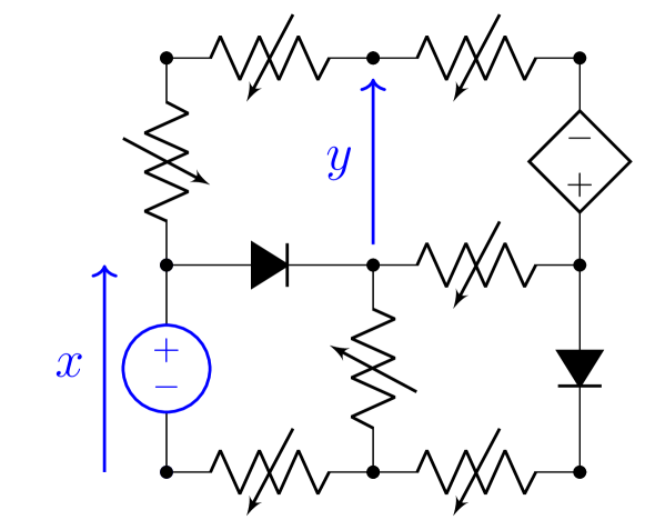
We call ‘nonlinear resistive network’ an electrical circuit composed of voltage sources, linear resistors, diodes and voltage-controlled voltage sources (Figure 1). A nonlinear resistive network can be utilized to implement input-output functions as follows: a) a set of voltage sources serve as ‘input variables’ where voltages play the role of input values, and b) a set of branches serve as ‘output variables’ where voltage drops play the role of the model’s prediction. Computing with this electrical network proceeds as follows:
-
1.
set the input voltage sources to input values,
-
2.
let the electrical network reach steady state (the DC operating point of the circuit),
-
3.
read the output voltages across output branches.
The steady state of the network is the configuration of branch voltages and branch currents that verifies all the branch equations, as well as Kirchhoff’s current law (KCL) at every node, and Kirchhoff’s voltage law (KVL) in every loop. We note that some conditions on the network topology and branch characteristics must be met to ensure that there exists a steady state: for instance, if the network contains a loop formed of voltage sources whose voltage values do not add up to zero, then KVL is violated. Subsequently, we will consider circuits that do not contain loops of voltage sources.
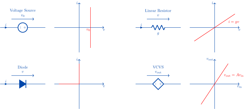
We assume that the above four circuit elements are ideal, meaning that their behaviour is determined by the following characteristics (see Figure 2):
-
•
The current-voltage (-) characteristic of a voltage source satisfies for some constant voltage value , regardless of the current .
-
•
A resistor follows Ohm’s law, i.e. its - characteristic is , where is the conductance ( where is the resistance).
-
•
The - characteristic of a diode satisfies for , and for .
-
•
A voltage-controlled voltage source (VCVS) has four terminals: two input terminals whose voltage we denote , and two output terminals whose voltage we denote . It satisfies the relationship , where is the ‘gain’ (or ‘amplification factor’).
Under these assumptions, nonlinear resistive networks are universal function approximators in the following sense.
Theorem 1 (A universal approximation theorem for nonlinear resistive networks).
Given any continuous function , and given any compact subset and any , there exists a nonlinear resistive network with input voltage sources and output branches such that, under the above assumptions of ideality, the function that it implements satisfies
| (1) |
The main aim of the next section is to prove Theorem 1.
3 Universal approximation through neural network approximation
To prove Theorem 1, we show that nonlinear resistive networks can approximate (artificial) neural networks to any desired accuracy. Since neural networks are universal approximators, it follows that nonlinear resistive networks are universal approximators, too.
We proceed in three steps. First, we recall the basic equations governing neural networks (Section 3.1). Then, we introduce a layered nonlinear resistive network model similar to the one proposed by Kendall et al. (2020) that we call ‘deep resistive network’ (DRN) and we derive the equations characterizing their steady state (Section 3.2). Finally, we prove that, under the assumptions of Section 2, any neural network can be approximated by a DRN (Section 3.3). Proofs of the Lemmas of this section are provided in Appendix A.
3.1 Deep neural network
An artificial neural network, or ‘deep neural network’ (DNN), is another (abstract) model of computation. DNNs have been extensively studied, and numerous theoretical results regarding their approximation capabilities exist. Within the deep learning literature, various types of DNNs are studied, but here we will use the following definition.
A DNN takes an input vector denoted as , sends it through multiple stages of transformations and produces an output vector. These stages of transformations are performed by the ‘layers’ of the network, which are themselves composed of ‘units’. We denote the number of layers and the number of units in layer , for each such that . The layer of index is called ‘input layer’ and the layer of index is called ‘output layer’. We further denote the state of unit in the -th layer. The equations defining the states of the units are the following. First, the states of input units are given by
| (2) |
where is the input vector. Next, the states of the units in the intermediate layers (), referred to as ’hidden’ layers, are defined by the following equation:
| (3) |
Finally, the states of output units are determined as:
| (4) |
In these equations, is the ‘weight’ connecting unit in layer to unit in layer , and represents the ‘bias’ associated with that unit. The function is commonly referred to as the ‘ReLU’ nonlinearity (Glorot et al., 2011). This neural network implements a function defined by for every .
It is known since the seminal works of Cybenko (1989); Hornik et al. (1989) that DNNs are universal approximators, meaning they can approximate arbitrary continuous functions.
Lemma 2 (DNNs are universal approximators).
Given any continuous function , and given any compact subset and any , there exists a neural network (DNN) with layers, input units and output units, such that the function that it implements satisfies
| (5) |
3.2 Deep resistive network
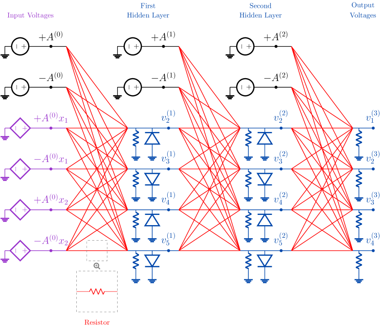
Next, we present a nonlinear resistive network model similar to the one of Kendall et al. (2020) that takes inspiration from the layered architecture of DNNs. We call it ‘deep resistive network’, or DRN.
In a DRN, the circuit elements - voltage sources, resistors and diodes - are assembled to form a layered network. A DRN is represented in Figure 3 and defined as follows. First of all, we choose a reference node called ‘ground’. We denote the number of layers in the DRN, and for each such that , we denote the number of nodes in layer . We choose input nodes and output nodes. We also call each node a ‘unit’ by analogy with the units of a neural network. We denote the electrical potential of the -th node of layer , which we may think of as the unit’s activation. Pairs of nodes from two consecutive layers are interconnected by (variable) resistors - the ‘trainable weights’. We denote the conductance of the resistor between the -th node of layer and the -th node of layer . The layer of index is the ‘input layer’, whose units are connected to ground by VCVS’s with the same gain . Moreover, there are voltage sources that play the role of input variables and serve as input voltages to the VCVS’s. Given an input vector , we set the input voltage sources to , so that the input nodes (VCVS output voltages) have electrical potentials
| (6) |
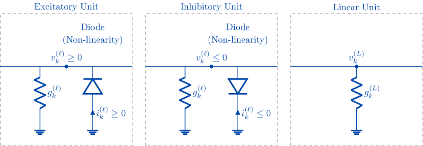
The units of intermediate (‘hidden’) layers () of the network are nonlinear: for each hidden unit, a diode is placed between the unit’s node and ground, which can be oriented in either of the two directions. For the units of even index , the diode points from the unit’s node to ground, so the unit’s electrical potential is non-negative: when it reaches , current flows through the diode from ground to the unit’s node so as to maintain the unit’s electrical potential at zero ; we call such a unit an excitatory unit. Conversely, for the units of odd index , the diode points from ground to the unit’s node, so the unit’s electrical potential is non-positive: when it reaches , the extra current sinks to ground through the diode ; we call it an inhibitory unit. Thus, half of the hidden units are excitatory and the other half are inhibitory. Output units are linear, meaning that no diode is used for the output units. Finally, each hidden and output unit is also linked to ground by a resistor whose conductance is denoted . In addition, each of the input and hidden layers contains a pair of ‘bias units’ that are connected to ground by voltage sources of fixed voltages:
| (7) |
where a layer-wise scalar – the ‘gain’ of layer .
Under the assumptions of ideality of the elements (Section 2), the steady state of the DRN - the configuration of branch voltages and branch currents that satisfies all the branch equations, as well as KCL and KVL - is determined by the following set of equations.
Lemma 3 (Equations of a DRN).
For every such that and , the equations for is
| (8) |
As for the equation of the output unit ,
| (9) |
A few remarks are in order. First, the equations characterizing the steady state of a DRN share similarities with those of a DNN: these equations also consist of weighted sum of the neighboring units’ activities (electrical potentials), and the function is the ‘ReLU’ nonlinearity.
However, these equations are not identical - a DRN is not a DNN. One difference is that, in a DRN, the units of a given layer receive signals not just from the previous layer but also from the next layer , in other words signals flow in both the forward and backward directions. Another difference is that these signals are normalized by the sum of the weights (total conductance) . We show below (Lemma 4) that, due to this, the layer-wise maximum amplitude of the electrical potentials, , satisfy the relationship , meaning that the signals decrease as the index of the layer () increases. This is the reason why voltage-controlled voltage sources (VCVS) are used: they amplify the input signals by a gain to compensate for the decay in amplitude and ensure that the signals at the output layer do not vanish.
Another difference between DRNs and DNNs is that the ‘weights’ of a DRN are non-negative - a conductance is non-negative - meaning . This is the reason why, in addition to excitatory units, we also use inhibitory units, so we can communicate ‘negative signals’ too. This is also the reason why we have doubled the number of input VCVS’s in the input layer (two VCVS’s for each input voltage source).
Lemma 4 (A maximum principle for DRNs).
For every such that , denote the maximum amplitude of electrical potential in layer as
| (10) |
Then we have
| (11) |
In particular, the electrical potentials of the units are bounded by the electrical potentials of input units:
| (12) |
3.3 Approximating a deep neural network with a deep resistive network
Given a DNN, we show that we can build a DRN (parametrized by a number ) that approximates the DNN. To this end, let be the number of layers of the DNN, and the number of units in layer , for . We denote and the weights and biases. Given an input vector , we also denote the state of the -th unit in layer of the DNN.
We build the DRN as follows. First we define its architecture. The DRN consists of layers and contains units in layer for and units in layer . It remains to choose the values of the conductances () and the amplification factors () for input and hidden layers. First we define for convenience . We also introduce a dimensionless number ; later we will let to establish the equivalence of the DRN and the DNN. For every triplet such that , and , we define
| (13) | |||
| (14) |
Furthermore, for every such that and , we define
| (15) |
We note that the conductances thus defined are all non-negative. Next, for every such that , we define
| (16) |
and for every such that and , we define
| (17) |
The conductances and are also non-negative, by definition of . Finally, we define the amplification factors for input and hidden layers
| (18) |
Lemma 5 (Approximation of a DNN with a DRN).
Suppose that, given an input signal , we set the input voltage sources to
| (19) |
Denote . Then, in the limit , we have:
| (20) | |||
| (21) |
Namely, when , the states of the excitatory units of the DRN tend to the states of the units of the DNN rescaled by . In particular, the states of output units of the DRN are equal to those of the DNN, up to . In other words, the function implemented by the DRN approximates the function implemented by the DNN.
Using a symmetry argument, one can prove that the DRN thus built has the property that for every . Although it might seem wasteful and redundant to have two units encode the same piece of information, we recall that doubling the number of units per layer (using excitatory and inhibitory units) is also what allows us to overcome the constraint of non-negative conductances in resistive networks.
Technically, due to the factor , since the conductances of layer are scaled by for each , the DRN behaves essentially as a feedforward model (DNN). Perhaps the most impractical assumption is that for deep networks the range of conductance values required will span over many orders of magnitude, proportional to the number of layers . It is noteworthy, however, that neural networks with a single hidden layer () are also universal approximators. For such a shallow network, the corresponding DRN will also have a single hidden layer, so the range of conductances will span few orders of magnitude only.
4 Discussion
Universal computation and universal approximation have been studied extensively in abstract models of computation such as deep neural networks (DNNs). In contrast, very little is known about the computational capabilities of physical systems. In this work, we have studied the representational power of resistor networks which utilize voltage sources as inputs and variable resistors as trainable weights. We have shown that, under suitable assumptions, electrical networks composed of voltage sources, resistors, diodes and voltage-controlled voltage sources (VCVS) can compute or approximate any continuous function. At the heart of our proof, we have shown that a DNN can be approximated by a deep resistive network (DRN). In particular, since DNNs are universal approximators, DRNs are also universal approximators.
While our theoretical result holds in principle, it entails assumptions. First, it is based on an assumption of ideality of the circuit elements. In particular, we assume ideal variable resistors whose conductances can be adjusted to arbitrary non-negative values - arbitrarily large or arbitrarily small. Similarly, we also require the ability to amplify input signals using VCVS’s whose amplification factors () can be potentially very large. Real-world variable resistors (or memristors), however, have quantized possible conductance values and evolve in a finite range. Besides, there is inherent noise in such electrical networks. For these reasons, the direct applicability of our constructive proof of Theorem 1 is unclear in practice. In particular, to build a practical DRN, we do not necessarily advise to rescale the weights of layer by a factor with .
Despite these assumptions, our theoretical result is a step towards better understanding resistor networks and their computational capabilities. It is known that these networks can be trained by gradient descent using local learning rules (Kendall et al., 2020; Anisetti et al., 2022) based on equilibrium propagation (Scellier and Bengio, 2017), and experimental realizations of such self-learning resistor networks have also been carried out (Dillavou et al., 2022, 2023). These features, together with their ability to approximate arbitrary continuous functions, make them an appealing alternative to conventional neural networks trained and deployed on GPUs. DRNs in particular, which take inspiration from the architecture of layered neural networks, present advantages in terms of hardware design, as they are potentially amenable for implementation using crossbar arrays of memristors (Xia and Yang, 2019).
Moving forward, our methodology based on the assumption of ideality of the circuit elements may be useful to further study and better understand the behaviour of nonlinear resistive networks. First, it could be useful to derive initialization schemes for the weights (conductances) in these networks, before training. Second, our methodlogy can also be used to derive efficient simulations of nonlinear resistive networks, which we leave for future work.
Finally, nonlinear resistive networks are closely related to continuous Hopfield networks (Hopfield, 1984). In particular, our proof, which shows that a DRN can behave as a DNN by rescaling the weights of layer by a factor , is similar to the one of Xie and Seung (2003) who showed that DNNs can be approximated by layered (continuous) Hopfield networks. The similarity between nonlinear resistive networks and continuous Hopfield networks is especially interesting as recent works have shown in computer simulations that such Hopfield networks can be trained with equilibrium propagation on the CIFAR10, CIFAR100 and ImageNet datasets, achieving promising results (Laborieux et al., 2021; Laborieux and Zenke, 2022; Scellier et al., 2023).
Acknowledgments and Disclosure of Funding
The authors thank Jack Kendall, Maxence Ernoult, Mohammed Fouda, Suhas Kumar, Vidyesh Anisetti, Andrea Liu, Axel Laborieux and Tim De Ryck for discussions.
References
- Anisetti et al. [2022] V. R. Anisetti, A. Kandala, B. Scellier, and J. Schwarz. Frequency propagation: Multi-mechanism learning in nonlinear physical networks. arXiv preprint arXiv:2208.08862, 2022.
- Cybenko [1989] G. Cybenko. Approximation by superpositions of a sigmoidal function. Mathematics of control, signals and systems, 2(4):303–314, 1989.
- Dillavou et al. [2022] S. Dillavou, M. Stern, A. J. Liu, and D. J. Durian. Demonstration of decentralized physics-driven learning. Physical Review Applied, 18(1):014040, 2022.
- Dillavou et al. [2023] S. Dillavou, B. Beyer, M. Stern, M. Z. Miskin, A. J. Liu, and D. J. Durian. Circuits that train themselves: decentralized, physics-driven learning. In AI and Optical Data Sciences IV, volume 12438, pages 115–117. SPIE, 2023.
- Glorot et al. [2011] X. Glorot, A. Bordes, and Y. Bengio. Deep sparse rectifier neural networks. In Proceedings of the fourteenth international conference on artificial intelligence and statistics, pages 315–323, 2011.
- Harris et al. [1989] J. Harris, C. Koch, J. Luo, and J. Wyatt. Resistive fuses: Analog hardware for detecting discontinuities in early vision. In Analog VLSI implementation of neural systems, pages 27–55. Springer, 1989.
- Hopfield [1984] J. J. Hopfield. Neurons with graded response have collective computational properties like those of two-state neurons. Proceedings of the national academy of sciences, 81(10):3088–3092, 1984.
- Hornik et al. [1989] K. Hornik, M. Stinchcombe, and H. White. Multilayer feedforward networks are universal approximators. Neural networks, 2(5):359–366, 1989.
- Kendall et al. [2020] J. Kendall, R. Pantone, K. Manickavasagam, Y. Bengio, and B. Scellier. Training end-to-end analog neural networks with equilibrium propagation. arXiv preprint arXiv:2006.01981, 2020.
- Kiraz et al. [2022] F. Z. Kiraz, D.-K. G. Pham, and P. Desgreys. Impacts of feedback current value and learning rate on equilibrium propagation performance. In 2022 20th IEEE Interregional NEWCAS Conference (NEWCAS), pages 519–523. IEEE, 2022.
- Laborieux and Zenke [2022] A. Laborieux and F. Zenke. Holomorphic equilibrium propagation computes exact gradients through finite size oscillations. arXiv preprint arXiv:2209.00530, 2022.
- Laborieux et al. [2021] A. Laborieux, M. Ernoult, B. Scellier, Y. Bengio, J. Grollier, and D. Querlioz. Scaling equilibrium propagation to deep convnets by drastically reducing its gradient estimator bias. Frontiers in neuroscience, 15:129, 2021.
- Lopez-Pastor and Marquardt [2023] V. Lopez-Pastor and F. Marquardt. Self-learning machines based on hamiltonian echo backpropagation. Physical Review X, 13(3):031020, 2023.
- Oh et al. [2023] S. Oh, J. An, S. Cho, R. Yoon, and K.-S. Min. Memristor crossbar circuits implementing equilibrium propagation for on-device learning. Micromachines, 14(7):1367, 2023.
- Scellier [2021] B. Scellier. A deep learning theory for neural networks grounded in physics. PhD thesis, Université de Montréal, 2021.
- Scellier and Bengio [2017] B. Scellier and Y. Bengio. Equilibrium propagation: Bridging the gap between energy-based models and backpropagation. Frontiers in computational neuroscience, 11:24, 2017.
- Scellier et al. [2023] B. Scellier, M. Ernoult, J. Kendall, and S. Kumar. Energy-based learning algorithms: A comparative study. In ICML Workshop on Localized Learning (LLW), 2023.
- Stern and Murugan [2023] M. Stern and A. Murugan. Learning without neurons in physical systems. Annual Review of Condensed Matter Physics, 14:417–441, 2023.
- Stern et al. [2022] M. Stern, S. Dillavou, M. Z. Miskin, D. J. Durian, and A. J. Liu. Physical learning beyond the quasistatic limit. Physical Review Research, 4(2):L022037, 2022.
- Stern et al. [2023] M. Stern, S. Dillavou, D. Jayaraman, D. J. Durian, and A. J. Liu. Physical learning of power-efficient solutions. arXiv preprint arXiv:2310.10437, 2023.
- Watfa et al. [2023] M. Watfa, A. Garcia-Ortiz, and G. Sassatelli. Energy-based analog neural network framework. Frontiers in Computational Neuroscience, 17:1114651, 2023.
- Wright et al. [2022] L. G. Wright, T. Onodera, M. M. Stein, T. Wang, D. T. Schachter, Z. Hu, and P. L. McMahon. Deep physical neural networks trained with backpropagation. Nature, 601(7894):549–555, 2022.
- Wycoff et al. [2022] J. F. Wycoff, S. Dillavou, M. Stern, A. J. Liu, and D. J. Durian. Desynchronous learning in a physics-driven learning network. The Journal of Chemical Physics, 156(14), 2022.
- Xia and Yang [2019] Q. Xia and J. J. Yang. Memristive crossbar arrays for brain-inspired computing. Nature materials, 18(4):309–323, 2019.
- Xie and Seung [2003] X. Xie and H. S. Seung. Equivalence of backpropagation and contrastive hebbian learning in a layered network. Neural computation, 15(2):441–454, 2003.
Appendix A Proofs
To prove the theoretical results, we proceed as follows. Lemma 2 is well known and admitted. First, we prove Lemma 3. Next, we prove Lemma 4 using Lemma 3. Then, we prove Lemma 5 using Lemma 3 and Lemma 4. Finally, we prove Theorem 1 using Lemma 2 and Lemma 5.
A.1 Proof of Lemma 3
For clarity, we repeat the lemma.
See 3
Proof of Lemma 3.
Consider unit in layer , with and . First we consider the case of a hidden layer (we will consider the case of the output layer later). We denote the current flowing through the diode to the unit’s node. The current flowing from ground to the unit’s node through the resistor is . We also denote the current flowing from the -th unit of layer to the -th unit of layer . Kirchhoff’s current law (KCL) applied to the -th unit of layer tells us that
| (22) |
Furthermore, by Ohm’s law we have and . Therefore
| (23) |
Solving (23) for we get
| (24) |
Now we use the characteristics of the diode between the unit’s node an ground. First we consider the case of an excitatory unit (). We distinguish between two sub-cases: either and (the diode is in ‘off-state’), or and (the diode is in ‘on-state’). In the first sub-case (off-state) we have, using (24)
| (25) |
In the second sub-case (on-state) we have, using (24) again,
| (26) |
From (25) and (26) it follows that both sub-cases are captured by a single formula:
| (27) |
Similarly, an inhibitory unit satisfies
| (28) |
The case of output nodes () is identical, with (meaning the layer of index is empty) and (no diode). Equation (24) rewrites in this case:
| (29) |
∎
A.2 Proof of Lemma 4
See 4
Proof of Lemma 4.
To prove (11), we proceed by induction on , starting from , down to . We start with . Using Lemma 3 we have for every ,
| (30) |
Since this holds for every (), it follows that
| (31) |
This completes the initialization step of the proof by induction. Suppose now that (11) holds for where and let’s show the property for . Using again Lemma 3:
| (32) | ||||
| (33) | ||||
| (34) |
Using the induction hypothesis, , we get
| (35) |
and since this holds for every , it follows that
| (36) |
Rearranging the terms, we get successively:
| (37) | ||||
| (38) | ||||
| (39) |
This completes the induction step, and therefore completes the proof. ∎
A.3 Proof of Lemma 5
See 5
Proof of Lemma 5.
We prove the property (20) by induction on . It is true for thanks to (19). Suppose that (20) is true for some and let us prove it at the rank . Let such that , and consider the excitatory unit (the case of inhibitory unit , and the case of linear output unit if , are similar). Recall from Lemma 3 that
| (40) |
First we calculate the denominator of expression (40). By distinguishing between the two cases or , it is easy to see that we have in both cases:
| (41) |
Summing from to , we get the following formula for the denominator in (40),
| (42) |
Next, we calculate the numerator of (40). Similarly, whether or , we have in both cases, using the inductive hypothesis:
| (43) |
This identity also holds for by defining to include the case of the biases. Therefore
| (44) |
Here we have used the maximum principle for (Lemma 4) to derive the bound . Finally, injecting (42) and (44) in (40) we obtain the following equation for :
| (45) |
The case of inhibitory unit is similar: we obtain
| (46) |
Hence, the property (20) is true at the rank . This completes the proof by induction. ∎
A.4 Proof of Theorem 1
See 1
Proof of Theorem 1.
Let be a continuous function. Let be a compact subset of , and let . By Lemma 2, there exists a neural network with inputs and outputs such that the function that it implements satisfies
| (47) |
Next, let , define and let the DRN approximator of with parameter (Section 3.3). By Lemma 5, the function implemented by satisfies
| (48) |
Combining the two equations, we obtain
| (49) |
Hence the result. ∎