One-loop five-parton amplitudes in the NMRK limit

Abstract

We analyse the real part of one-loop five-parton amplitudes in the next-to-multi-Regge kinematic (NMRK) limit, to leading power, and to finite order in the dimensional regularisation parameter. To leading logarithmic (LL) accuracy, it is known that five-parton amplitudes in this limit are given to all-orders by a single factorised expression, in which the pair of partons which are not well-separated in rapidity are described by a two-parton emission vertex. In this study, we investigate the one-loop amplitudes at next-to-leading logarithmic (NLL) accuracy, and find that is has a more complex structure. In particular, it is found that the purely gluonic amplitudes are compatible with an analogous factorisation of individual colour structures. From the one-loop amplitudes we extract one-loop two-parton emission vertices, which are functions of a subset of the momenta of the amplitude. In the multi-Regge kinematic (MRK) limit, the vertices themselves factorise into the known one-loop single-parton emission vertices and Lipatov vertex, with rapidity dependence governed by the one-loop gluon Regge trajectory, as required by compatibility with the known MRK limit of amplitudes. The one-loop two-parton emission vertices are necessary ingredients for the construction of the next-to-next-to leading order (NNLO) jet impact factors in the BFKL framework.

1 Introduction

The multi-Regge kinematic (MRK) limit of amplitudes, in which final-state particles are strongly ordered in rapidity, has long been a source of insight into the all-orders structure of amplitudes Lipatov:1976zz ; DelDuca:2019tur . Knowledge of the MRK limit has been used to compute or constrain amplitudes in general kinematics DelDuca:2009au ; DelDuca:2010zg ; Dixon:2014iba ; Henn:2016jdu ; Caron-Huot:2016owq ; Almelid:2017qju ; Caron-Huot:2019vjl ; Falcioni:2021buo ; Caola:2021izf . Historically, the next-to-multi-Regge kinematic (NMRK) limit (or single-Regge limit), where one of the strong rapidity-ordering requirements is relaxed, has received far less attention than the more tractable MRK limit, with some notable exceptions, including refs. White:1973ola ; Brower:1974yv . The NMRK limit is an intriguing theoretical arena, where on the one hand the simplified kinematics make possible a detailed study of high-multiplicity amplitudes, revealing structures which are obscured in general kinematics Bartels:2008ce ; Byrne:2022wzk , and on the other hand, the NMRK limit captures more of the complexity and richness of amplitudes than does the MRK limit. The NMRK limit and its MRK boundaries provide an ideal test bed for studying which properties of MRK amplitudes generalise to more generic kinematic spaces. In this work, we find that the known MRK limit of amplitudes motivates a highly convenient framework for organising the kinematic structure of the amplitudes in the NMRK limit. In particular, this organisation makes it trivial to take the further MRK limit of NMRK-factorised expressions.

The behaviour of amplitudes in Regge limits is important for determining the asymptotic high-energy limit of cross sections in QCD Lipatov:1976zz ; Kuraev:1976ge . The leading-logarithmic (LL) behaviour of amplitudes in QCD is described by the $t$-channel exchange of a so-called Reggeised gluon. In the language of Regge theory (for pedagogical reviews see refs. Collins:1977jy ; White:2019ggo ; Mizera:2023tfe ), the amplitude is governed by a simple Regge pole in the complex angular momentum plane. The Balitsky-Fadin-Kuraev-Lipatov (BFKL) equation Lipatov:1976zz ; Kuraev:1976ge ; Kuraev:1977fs ; Balitsky:1978ic sums the LL contributions to QCD scattering processes to all orders in the coupling (for pedagogical introductions see refs. DelDuca:1995hf ; Forshaw:1997dc ; Fadin:1998sh ). The leading order (LO) kernel of this equation consists of the square of the Lipatov vertex Lipatov:1976zz , which can be obtained by taking the MRK limit of tree-level amplitudes. At next-to-leading logarithmic (NLL) accuracy, the real part of amplitudes are similarly described by a simple Regge pole Fadin:2006bj ; Fadin:2015zea , which allows the BFKL approach to be extended to NLL accuracy Fadin:1998py ; Ciafaloni:1998gs ; Kotikov:2000pm ; Kotikov:2002ab . This requires the kernel to be extended to next-to-leading order (NLO). The NLO kernel may be computed using building blocks which can be obtained by taking the MRK limit of one-loop amplitudes as well as building blocks which can be obtained by taking the NMRK limit of tree-level amplitudes. At next-to-next-to leading-logarithmic (NNLL) accuracy, the real part of the amplitude is described by a Regge cut in addition to a Regge pole Fadin:2020lam ; Caron-Huot:2017fxr ; DelDuca:2001gu ; Fadin:2017nka . Recently, schemes have been introduced to disentangle the pole and cut contributions at fixed order Falcioni:2021dgr ; Fadin:2021csi . In particular, the three-loop Regge trajectory has recently been determined DelDuca:2021vjq ; Caola:2021izf ; Caola:2022dfa . It is hoped that the BFKL approach may yet be extended to describe the evolution of the Regge-pole contribution.

As reviewed in ref. Byrne:2022wzk , there has been much progress towards extending the BFKL approach to NNLL accuracy. More recently, knowledge of the one-loop Lipatov vertex has been extended to ${\mathcal{O}}(\epsilon^{2})$ Fadin:2023roz , as required for the NNLO kernel, and the recent calculation of two-loop five-parton amplitudes in QCD Agarwal:2023suw ; DeLaurentis:2023nss ; DeLaurentis:2023izi has made possible the extraction of the two-loop Lipatov vertex.

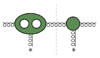
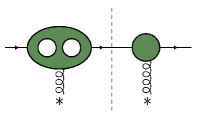
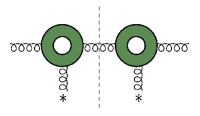
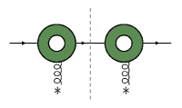
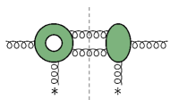
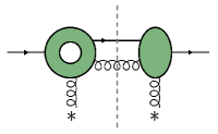
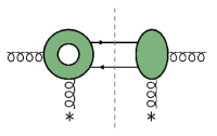
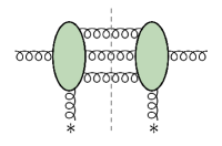
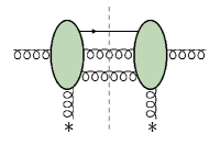
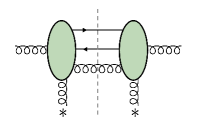
Figure 1: Ingredients of the NNLO jet impact factors: (a)-(d) double-virtual corrections; (e)-(g) real-virtual corrections; (h)-(j) double-real corrections. Punctures in blobs denote loop corrections. An asterisk indicates an off-shell gluon. The grey dashed line indicates the final-state cut.

In order to provide NNLL accurate predictions for physical processes it is necessary to also know not only the kernel, but also the relevant impact factors to NNLO accuracy. Let us briefly review the current status of the NNLO impact factors for the production of a jet, which are depicted in fig. 1. The double-virtual corrections to the impact factors (figs. 1, 1, 1 and 1) require knowledge of the two-loop single-parton peripheral-emission vertices DelDuca:2014cya as well as the interference of two one-loop single-parton peripheral-emission vertices Fadin:1992rh ; Fadin:1992zt ; Fadin:1995km ; DelDuca:1998kx . The double-real corrections to the impact factors (figs. 1, 1 and 1) require knowledge of the three-parton emission vertices. These are known for the pure-gluon case DelDuca:1999iql ; Antonov:2004hh ; Duhr:2009uxa , but the tree-level ${\bar{q}}qggg^{*}$ vertices are not yet known. In this paper we obtain some of the missing ingredients for the real-virtual correction to the impact factors (figs. 1, 1 and 1), namely the one-loop two-parton peripheral-emission vertices for both the $gggg^{*}$ and ${\bar{q}}qgg^{*}$ case. The one-loop $gggg^{*}$ vertex has previously been determined for two colour-orderings and helicity-independence of this vertex was incorrectly assumed Canay:2021yvm . In section 6 we clarify the need for determining a third distinct colour ordering of this vertex, and in section 7 we show that two distinct helicity configurations of this vertex are required for the NNLO impact factor.

To regulate the infra-red divergences which will appear when performing the phase space integration of the two-parton emission vertices it will be necessary to know the one-loop two-parton peripheral-emission vertices to order $\epsilon$ in the soft and collinear limits and to order $\epsilon^{2}$ in the soft-collinear limit. In this paper we focus exclusively on finite (${\mathcal{O}}(\epsilon^{0})$) corrections, which can be inferred from available one-loop amplitudes Bern:1993mq ; Bern:1994fz . These amplitudes already reveal some interesting structure of amplitudes in the NMRK limit beyond tree-level. We find that, in contrast to the tree-level amplitudes, the one-loop amplitudes are not compatible with an all-orders factorisation of the amplitude. Rather, they are at best compatible with an all-orders factorisation of two different colour structures of the amplitude.

The one-loop two-parton emission vertices also contain additional colour structures compared to the tree-level vertices. For the $gggg^{*}$ vertex, this is a totally symmetric colour structure, while for the ${\bar{q}}qgg^{*}$ vertex it is a product of delta functions in the adjoint and fundamental representations. In the latter case, the new colour structure survives interference with the tree-level vertex, hence contributes to the NNLO kernel.

The factorisation-structure and colour-structure of the ${\mathcal{N}}{=}4$ part of the one-loop $gggg^{*}$ is analogous to the structure of the ${\mathcal{N}}{=}4$ $g^{*}ggg^{*}$ vertex obtained in ref. Byrne:2022wzk . We expect the one-loop $g^{*}ggg^{*}$ and $g^{*}{\bar{q}}qg^{*}$ vertices in QCD to have analogous structure to the $gggg^{*}$ and ${\bar{q}}qgg^{*}$ vertices presented in this work.

The structure of this paper is as follows. In section 2 we review the relevant properties of QCD amplitudes in the high-energy limit. In section 3 we introduce a minimal set of kinematic variables to describe $2\to 3$ scattering which we will use throughout the paper. In section 4 we will review the properties of tree-level five-parton amplitudes in the NMRK limit and in section 5 we will review the properties of one-loop four parton amplitudes in the Regge limit. These two chapters provide the necessary background for the study of one-loop five-parton amplitudes, which is the topic of the remaining chapters. In section 6 we study the colour structure of one-loop five-parton amplitudes at leading power in the NMRK limit. In section 7 and section 8 we study the respective factorisation properties of colour-ordered and colour-dressed one-loop five-gluon amplitudes in the NMRK limit. In section 9 and section 10 we perform the analogous studies of one-loop five-parton amplitudes with an external quark-antiquark pair. Finaly, we conclude in section 11.

2 Review of high-energy limit of amplitudes in QCD

Our conventions for general kinematics are given in section A.1 and our notation for kinematics in Regge limits is given in section A.2. In this section we briefly review the all-orders structure of amplitudes in the Regge limit, given by eq. 292. At tree-level, amplitudes are dominated by the $t$-channel exchange of a gluon, and to leading power have the factorised form Lipatov:1976zz ; Kuraev:1976ge

$$\begin{split}\mathcal{A}_{4}^{(0)}(f_{2}^{\lambda_{2}},f_{3}^{\lambda_{3}},f_{4}^{\lambda_{3}},f_{1}^{\lambda_{3}})&\underset{\mathrm{Regge}}{\to}2s\ \mathcal{C}^{(0)}_{f_{2}f_{3}g^{*}}(p_{2}^{\lambda_{2}},p_{3}^{\lambda_{3}},q)\ \frac{1}{t}\ \mathcal{C}^{(0)}_{g^{*}f_{4}f_{1}}(-q,p_{4}^{\lambda_{4}},p_{1}^{\lambda_{1}})\,.\end{split}$$ (1)

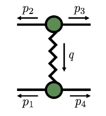
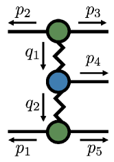
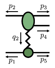
Figure 2: Illustrations of the factorised forms of amplitudes discussed in the text: (a) factorisation of the $2\to 2$ amplitude in the Regge limit; (b) factorisation of the $2\to 3$ amplitude in the MRK limit; (c) factorisation of the $2\to 3$ amplitude in the forward NMRK limit. The green and blue blobs denote peripheral- and central-emission vertices respectively, to all orders in the coupling $g_{\mathrm{s}}$. The solid external lines denote the permitted parton types, as given in the main text. The zig-zag lines denote a Reggeised gluon.

All the process-dependent information is contained in the vertices, which are only non-zero when the representation of the external partons permits the $t$-channel exchange of an anti-symmetric octet:

$$\mathcal{C}^{(0)}_{ggg^{*}}(p_{2}^{\lambda_{2}},p_{3}^{\lambda_{3}},q) =g_{\mathrm{s}}\,(F^{c})_{a_{2}a_{3}}\,C^{(0)}_{ggg^{*}}(p_{2}^{\lambda_{2}},p_{3}^{\lambda_{3}},q)\,,$$ (2a)

$$\mathcal{C}^{(0)}_{{\bar{q}}qg^{*}}(p_{2}^{\lambda_{2}},p_{3}^{\lambda_{3}},q) =g_{\mathrm{s}}\,(T^{c})_{\imath_{3}\bar{\imath}_{2}}\,C^{(0)}_{{\bar{q}}qg^{*}}(p_{2}^{\lambda_{2}},p_{3}^{\lambda_{3}},q)\,.$$ (2b)

Here $T$ are generators in the fundamental representation of $SU(N_{c})$ with normalisation $\mbox{tr}\left(T^{a}T^{b}\right)=\delta_{ab}$. The structure constants, $f$, follow from the commutatation relation

$$[T^{a},T^{b}]_{ij}=if^{abc}\,T^{c}_{ij}.$$ (3)

We often make use of the notation $(F^{b})_{ac}=if^{abc}$ for generators in the adjoint representation, whereby the Jacobi identity is

$$[F^{a},F^{b}]_{d_{i}d_{j}}=if^{abc}F^{c}_{d_{i}d_{j}}.$$ (4)

Equation 2 introduces several conventions we use throughout this paper. In order to emphasise the analogy between amplitudes and factorised vertices we have listed the three outgoing momenta of the vertices. Although this is redundant, as the vertices conserve momentum, this notation will be helpful when keeping track of the colour-orderings of higher-multiplicity vertices. For amplitudes and vertices alike, we use caligraphic type for colour-dressed objects and roman type for colour-stripped objects. In the case of eq. 2, the colour-stripped vertices are simply helicity conserving phases. Using the conventions of section A.1, these phases are DelDuca:1995zy ; DelDuca:1996km

$$C^{(0)}_{ggg^{*}}(p_{2}^{\ominus},p_{3}^{\oplus},q) =1\,,\qquad C^{(0)}_{g^{*}gg}(-q,p_{4}^{\oplus},p_{1}^{\ominus})=-\frac{q_{\perp}^{*}}{q_{\perp}}\,,$$ (5a)

$$C^{(0)}_{{\bar{q}}qg^{*}}(p_{2}^{\ominus},p_{3}^{\oplus},q) =1\,,\qquad C^{(0)}_{g^{*}{\bar{q}}q}(-q,p_{4}^{\oplus},p_{1}^{\ominus})=\left(\frac{q_{\perp}^{*}}{q_{\perp}}\right)^{\frac{1}{2}}\,.$$ (5b)

The vertices are antisymmetric under $p_{2}^{\lambda_{2}}\leftrightarrow p_{3}^{\lambda_{3}}$ or $p_{4}^{\lambda_{4}}\leftrightarrow p_{1}^{\lambda_{1}}$, and parity conjugation of the vertices is given by complex conjugation. To leading-logarithmic (LL) accuracy in $\frac{s}{t}$, the amplitudes are given to all-orders by the factorised form Lipatov:1976zz ; Kuraev:1976ge

$$\begin{split}\mathcal{A}_{4}(f_{2}^{\lambda_{2}},f_{3}^{\lambda_{3}},f_{4}^{\lambda_{3}},f_{1}^{\lambda_{3}})&\underset{\mathrm{Regge}}{\to}2s\ \mathcal{C}^{(0)}_{f_{2}f_{3}g^{*}}(p_{2}^{\lambda_{2}},p_{3}^{\lambda_{3}},q)\ \frac{1}{t}\left(\frac{s}{\tau}\right)^{\alpha(t)}\ \mathcal{C}^{(0)}_{g^{*}f_{4}f_{1}}(-q,p_{4}^{\lambda_{4}},p_{1}^{\lambda_{1}})\,,\end{split}$$ (6)

which is illustrated in fig. 2. Here $\tau$ is some positive scale of the order $t$. We consider the amplitude to have the expansion in the bare coupling $g_{\mathrm{s}}$,

$$\mathcal{A}_{4}=\mathcal{A}_{4}^{(0)}+\mathcal{A}_{4}^{(1)}+{\cal O}(g_{\mathrm{s}}^{6})\,,$$ (7)

where the superscript $(l)$ denotes the loop-order and $\mathcal{A}^{(l)}_{4}\sim{\cal O}(g_{\mathrm{s}}^{2(1+l)})$. In eq. 6, the virtual corrections are given to all orders by the exponentiation of the one-loop Regge trajectory Lipatov:1976zz ; Kuraev:1976ge

$$\alpha^{(1)}(t)=c_{\Gamma}\ g_{\mathrm{s}}^{2}\ \frac{2N_{c}}{\epsilon}\left(\frac{\mu^{2}}{-t}\right)^{\epsilon}\,,$$ (8)

where $c_{\Gamma}$ is the ubiquitous loop factor

$$c_{\Gamma}=\frac{1}{(4\pi)^{2-\epsilon}}\frac{\Gamma(1+\epsilon)\Gamma(1-\epsilon)^{2}}{\Gamma(1-2\epsilon)}\,.$$ (9)

Beyond LL, it is useful to introduce the concept of signature, or symmetry under crossing $s\leftrightarrow u$. In the Regge limit this is equivalent to $s\leftrightarrow-s$, and signature-even ($[+]$) and signature-odd ($[-]$) ampltiudes are given by

$$\begin{split}\mathcal{A}_{4}^{[\pm]}(s,t)=\frac{1}{2}\Big{(}&\mathcal{A}_{4}(s,t)\pm\mathcal{A}_{4}(-s,t)\Big{)}\,.\end{split}$$ (10)

At NLL, a factorised form analogous to eq. 6 only holds for the signature-odd amplitude. The generalisation of eq. 6 to NLL accuracy is Caron-Huot:2017fxr ; Fadin:1993wh

$$\begin{split}{\mathrm{Disp}\left[{\mathcal{A}^{[-]}_{4}(f_{2}^{\lambda_{2}},f_{3}^{\lambda_{3}},f_{4}^{\lambda_{4}},f_{1}^{\lambda_{1}})}\right]}&\underset{\mathrm{Regge}}{\to}2s\ \mathcal{C}_{f_{2}f_{3}g^{*}}(p_{2}^{\lambda_{2}},p_{3}^{\lambda_{3}},q)\ \mathcal{R}_{g^{*}}(q;s)\ \mathcal{C}_{g^{*}f_{4}f_{1}}(-q,p_{4}^{\lambda_{4}},p_{1}^{\lambda_{1}})\,.\end{split}$$ (11)

In this paper we only consider the dispersive part of amplitudes, defined by taking the real part of the transcendental functions. For $2\to 2$ scattering the Regge cut starts to contribute to the absorptive part of the signature-even amplitude at one-loop, and (beyond the planar limit) to the dispersive part of the signature-odd amplitude at two-loops Falcioni:2021dgr . As outlined in the introduction, our interest is in the Regge-pole contribution to the amplitude, so we limit our analysis to the dispersive part of the signature-odd amplitude. In eq. 11 we have introduced the notation

$$\mathcal{R}_{g^{*}}(q;s)=\frac{1}{t}\times\frac{1}{2}\ \Bigg{[}\bigg{(}\frac{s}{\tau}\bigg{)}^{\alpha(t)}+\bigg{(}\frac{-s}{\tau}\bigg{)}^{\alpha(t)}\Bigg{]}\,,$$ (12)

for a signature-even Reggeisation factor. This factor is relevant for the signature-odd amplitude due to the overall factor of $s$ in eq. 11. We consider the factorised terms in eq. 11 to have an expansion in the coupling. At NLL we need to consider the expansion of the peripheral-emission vertices to one loop,

$$\mathcal{C}_{f_{2}f_{3}g^{*}}(p_{2}^{\lambda_{2}},p_{3}^{\lambda_{3}},q)=\mathcal{C}^{(0)}_{f_{2}f_{3}g^{*}}(p_{2}^{\lambda_{2}},p_{3}^{\lambda_{3}},q)+\mathcal{C}^{(1)}_{f_{2}f_{3}g^{*}}(p_{2}^{\lambda_{2}},p_{3}^{\lambda_{3}},q)+\mathcal{O}\left(g_{\mathrm{s}}^{5}\right)$$ (13)

with the (unrenormalised) one-loop correction to eq. 2a given by Fadin:1992rh ; Fadin:1992zt ; DelDuca:1998kx

$$\mathcal{C}^{(1)}_{ggg^{*}}(p_{2}^{\oplus},p_{3}^{\ominus},q)=g_{\mathrm{s}}^{3}\,c_{\Gamma}\,F^{c}_{a_{2}a_{3}}\,C^{(0)}_{ggg^{*}}(p_{2}^{\oplus},p_{3}^{\ominus},q)$$ (14a)

$$\times\Bigg{\{}\left(\frac{\mu^{2}}{-t}\right)^{\epsilon}\left[N_{c}\left(-\frac{2}{\epsilon^{2}}-\frac{11}{6\varepsilon}+\frac{1}{\varepsilon}\log\left(\frac{\tau}{-t}\right)-\frac{32}{9}-\frac{\delta_{R}}{6}+\frac{\pi^{2}}{2}\right)+N_{f}\left(\frac{1}{3\varepsilon}+\frac{5}{9}\right)\right]\Bigg{\}}$$

and the (unrenormalised) one-loop correction to eq. 2b given by Fadin:1995km ; DelDuca:1998kx

$$\mathcal{C}^{(1)}_{{\bar{q}}qg^{*}}(p_{2}^{\oplus},p_{3}^{\ominus},q)=g_{\mathrm{s}}^{3}\,c_{\Gamma}\,T^{c}_{\imath_{3}\bar{\imath}_{2}}\,C^{(0)}_{{\bar{q}}qg^{*}}(p_{2}^{\oplus},p_{3}^{\ominus},q)$$ (14b)

$$\times\Bigg{\{}\left(\frac{\mu^{2}}{-t}\right)^{\epsilon}\bigg{[}N_{c}\left(-\frac{1}{\epsilon^{2}}+\frac{1}{3\epsilon}+\frac{1}{\varepsilon}\log\left(\frac{\tau}{-t}\right)+\frac{19}{18}-\frac{\delta_{R}}{3}+\frac{\pi^{2}}{2}\right)-N_{f}\left(\frac{1}{3\epsilon}+\frac{5}{9}\right)$$

$$\qquad+\frac{1}{N_{c}}\left(\frac{1}{\epsilon^{2}}+\frac{3}{2\epsilon}+\frac{7}{2}+\frac{\delta_{R}}{2}\right)\bigg{]}.$$

The above vertices are written in terms of the regularisation parameter $\delta_{R}$, where $\delta_{R}=1$ in CDR/HV schemes and $\delta_{R}=0$ in the DR/FDH schemes Catani:1996pk . In the following, because we will adopt an organisation of amplitudes into supersymmetric multiplets, we set $\delta_{R}=0$. At one-loop the helicity-violating $ggg^{*}$ vertex Fadin:1993qb ; DelDuca:1998kx ,

$$\begin{split}\mathcal{C}^{(1)}_{ggg^{*}}(p_{2}^{\oplus},p_{3}^{\oplus},q)&=g_{\mathrm{s}}^{3}F^{c}_{a_{2}a_{3}}(N_{c}-N_{f})\frac{1}{3(4\pi)^{2}}\left(\frac{-q_{\perp}^{*}}{q_{\perp}}\right)\,,\end{split}$$ (15a)

$$\begin{split}\mathcal{C}^{(1)}_{ggg^{*}}(p_{4}^{\oplus},p_{1}^{\oplus},q)&=g_{\mathrm{s}}^{3}F^{c}_{a_{4}a_{1}}(N_{c}-N_{f})\frac{1}{3(4\pi)^{2}}\,,\end{split}$$ (15b)

also contributes at leading-power in the Regge limit. This vertex did not contribute to the NLO impact factors, but the square of eq. 15 does contribute to the NNLO impact factors.

In eq. 11 we must also consider the expansion of the Regge trajectory to two loops,

$$\alpha(t)=\alpha^{(1)}(t)+\alpha^{(2)}(t)+\mathcal{O}\left(g_{\mathrm{s}}^{6}\right)\,,$$ (16)

but as the subject of this paper is the analysis of one-loop amplitudes, we will only need eq. 8. The expansion eq. 16 is equivalent to an expansion of the Reggeised propagator,

$$\mathcal{R}_{g^{*}}(q;s)=\mathcal{R}_{g^{*}}^{(0)}(q)+\mathcal{R}_{g^{*}}^{(1)}(q;s)+\mathcal{O}\left(g_{\mathrm{s}}^{3}\right)\,.$$ (17)

As for the vertices, eq. 2, it is useful to consider the kinematic part of eq. 17, stripped of colour factors and coupling constants, that is

$$\mathcal{R}^{(0)}_{g^{*}}(q) =R^{(0)}_{g^{*}}(q)\,,$$ (18)

$$\mathcal{R}^{(1)}_{g^{*}}(q;s) =g_{\mathrm{s}}^{2}\,N_{c}\,R^{(1)}_{g^{*}}(q;s)\,,$$ (19)

where for clarity, we list the colour-stripped factors at tree-level and one-loop accuracy:

$$R^{(0)}_{g^{*}}(q) =\frac{1}{t}\,,$$ (20)

$$R^{(1)}_{g^{*}}(q;s) =c_{\Gamma}\frac{1}{t}\frac{2}{\epsilon}\left(\frac{\mu^{2}}{t}\right)^{\epsilon}\log\left(\frac{s}{\tau}\right)\,.$$ (21)

The factorised form of eq. 11 generalises beyond the $2\to 2$ case, for example, the MRK limit of the $2\to 3$ amplitude (eq. 293) is Lipatov:1976zz ; Kuraev:1976ge

$$\begin{split}{\mathrm{Disp}\left[{\mathcal{A}_{5}^{[-,-]}\left(f_{2}^{\lambda_{2}},f_{3}^{\lambda_{3}},g_{4}^{\lambda_{4}},f_{5}^{\lambda_{5}},f_{1}^{\lambda_{1}}\right)}\right]}\underset{\scriptscriptstyle{\mathrm{MRK}}}{\to}2s\ &\mathcal{C}_{f_{2}f_{3}g^{*}}(p_{2}^{\lambda_{2}},p_{3}^{\lambda_{3}},q_{1})\ \mathcal{R}_{g^{*}}(q_{1};s_{34})\\ \times&\mathcal{V}_{g^{*}gg^{*}}(-q_{1},p_{4}^{\lambda_{4}},q_{2})\\ \times&\mathcal{R}_{g^{*}}(q_{2};s_{45})\ \mathcal{C}_{g^{*}f_{5}f_{1}}(-q_{2},p_{5}^{\lambda_{5}},p_{1}^{\lambda_{1}})\,,\end{split}$$ (22)

which is valid to LL accuracy at amplitude level. Here the amplitude consists of antisymmetric colour representations exchanged in both $t_{1}$ and $t_{2}$ channels. As above, we restrict our study to the dispersive part of the ampltiude. The phases of amplitudes in the MRK are properly treated with the analytic representation of amplitudes given in refs. Fadin:1993wh ; Bartels:1980pe ; Bartels:2008ce but eq. 22 is sufficient for our present purposes.

The central-emission vertex has an expansion in the coupling, analogous to eq. 13. In the present work we will need to know this vertex to one-loop accuracy,

$$\begin{split}\mathcal{V}_{g^{*}gg^{*}}(-q_{1},p_{4}^{\lambda_{4}},q_{2})=\mathcal{V}_{g^{*}gg^{*}}^{(0)}(-q_{1},p_{4}^{\lambda_{4}},q_{2})+\mathcal{V}_{g^{*}gg^{*}}^{(1)}(-q_{1},p_{4}^{\lambda_{4}},q_{2})+\mathcal{O}\left(g_{\mathrm{s}}^{5}\right)\,.\end{split}$$ (23)

The leading-order Lipatov vertex is given by

$$\begin{split}\mathcal{V}_{g^{*}gg^{*}}^{(0)}(-q_{1},p_{4}^{\lambda_{4}},q_{2})&=i\,g_{\mathrm{s}}\,f^{c_{1}c_{2}a_{4}}\,V_{g^{*}gg^{*}}^{(0)}(-q_{1},p_{4}^{\lambda_{4}},q_{2})\,,\\ \end{split}$$ (24)

with colour-stripped vertex

$$\begin{split}V^{(0)}_{g^{*}gg^{*}}(-q_{1},p_{4}^{\lambda_{4}},q_{2})&=\frac{q_{1\perp}^{\ast}q_{2\perp}}{p_{4\perp}}\,,\\ \end{split}$$ (25)

and the (unrenormalised) one-loop Lipatov vertex is given by Fadin:1993wh ; Fadin:1994fj ; DelDuca:1998cx

$$\begin{split}&\mathcal{V}_{g^{*}gg^{*}}^{(1)}(-q_{1},p_{4}^{\oplus},q_{2})=i\,c_{\Gamma}\,g_{\mathrm{s}}^{3}\,f^{c_{1}c_{2}a_{4}}\,V_{g^{*}gg^{*}}^{(0)}(-q_{1},p_{4}^{\lambda_{4}},q_{2})\\ &\times\Bigg{\{}N_{c}\bigg{[}-\frac{1}{\epsilon^{2}}\left(\frac{\mu^{2}}{\left|p_{4\perp}\right|^{2}}\right)^{\epsilon}+\frac{1}{\epsilon}\left(\left(\frac{\mu^{2}}{-t_{1}}\right)^{\epsilon}+\left(\frac{\mu^{2}}{-t_{2}}\right)^{\epsilon}\right)\log\left(\frac{\tau}{\left|p_{4\perp}\right|^{2}}\right)-\frac{1}{2}\log^{2}\left(\frac{t_{1}}{t_{2}}\right)+\frac{\pi^{2}}{3}\bigg{]}\\ &\qquad-\frac{\beta_{0}}{2}\left(t_{1}+t_{2}+2q_{1\perp}q_{2\perp}^{*}\right)\frac{L_{0}\left(t_{1}/t_{2}\right)}{t_{2}}\\ &\qquad-\frac{(N_{c}-N_{f})}{3}\left|p_{4\perp}\right|^{2}\left[\left(2t_{1}t_{2}+\left(t_{1}+t_{2}+2\left|p_{2\perp}\right|^{2}\right)q_{1\perp}q_{2\perp}^{*}\right)\frac{L_{2}\left(t_{1}/t_{2}\right)}{t_{2}^{3}}+\frac{q_{1\perp}q_{2\perp}^{*}}{2t_{1}t_{2}}\right]\Bigg{\}}\,.\end{split}$$ (26)

The $L_{i}$ functions are defined in appendix B, and the coefficient of the one-loop beta function in QCD is

$$\beta_{0}=\frac{11N_{c}-2N_{f}}{3}\,.$$ (27)

In this paper we are concerned with the factorisation of amplitudes in the NMRK limit, eq. 294. The factorised form

$$\begin{split}{\mathrm{Disp}\left[{\mathcal{A}_{5}^{[-]}\left(f_{2}^{\lambda_{2}},f_{3}^{\lambda_{3}},f_{4}^{\lambda_{3}},f_{5}^{\lambda_{5}},f_{1}^{\lambda_{1}}\right)}\right]}\underset{\scriptscriptstyle{\mathrm{NMRK}}}{\to}2s\ &\mathcal{C}_{f_{2}f_{3}f_{4}g^{*}}(p_{2}^{\lambda_{2}},p_{3}^{\lambda_{3}},p_{4}^{\lambda_{4}},q_{2})\\ \times&\mathcal{R}_{g^{*}}(q_{2};s_{45})\\ \times&\mathcal{C}_{g^{*}f_{5}f_{1}}(-q_{2},p_{5}^{\lambda_{5}},p_{1}^{\lambda_{1}})\,,\end{split}$$ (28)

is valid to LL accuracy, as detailed in section 4. Here the superscript $[-]$ now denotes the exchange of anti-symmetric colour representations in just the $t_{2}$ channel. In this paper we investigate whether eq. 28 holds also to NLL accuracy, which would allow us to define a one-loop correction to the two-parton emission vertex of the form

$$\mathcal{C}^{(1)}_{f_{2}f_{3}f_{4}g^{*}}(p_{2}^{\lambda_{2}},p_{3}^{\lambda_{3}},p_{4}^{\lambda_{4}},q_{2}).$$

We impose the requirement that this vertex factorises in the further MRK and ${\mathrm{MRK}^{\prime}}$ limits according to eq. 22, i.e.

$$\mathcal{C}_{f_{2}f_{3}f_{4}g^{*}}(p_{2}^{\lambda_{2}},p_{3}^{\lambda_{3}},p_{4}^{\lambda_{4}},q_{2}) \underset{y_{3}\gg y_{4}}{\to}\mathcal{C}_{f_{2}f_{3}g^{*}}(p_{2}^{\lambda_{2}},p_{3}^{\lambda_{3}},q_{1})\mathcal{R}_{g^{*}}(q_{1};s_{34})\mathcal{V}_{g^{*}gg^{*}}^{(0)}(-q_{1},p_{4}^{\lambda_{4}},q_{2})\,,$$ (29)

$$\mathcal{C}_{f_{2}f_{3}f_{4}g^{*}}(p_{2}^{\lambda_{2}},p_{3}^{\lambda_{3}},p_{4}^{\lambda_{4}},q_{2}) \underset{y_{4}\gg y_{3}}{\to}\mathcal{C}_{f_{2}f_{4}g^{*}}(p_{2}^{\lambda_{2}},p_{4}^{\lambda_{4}},q_{1}^{\prime})\mathcal{R}_{g^{*}}(q_{1}^{\prime};s_{43})\mathcal{V}_{g^{*}gg^{*}}^{(0)}(-q_{1}^{\prime},p_{3}^{\lambda_{3}},q_{2})\,,$$ (30)

whenever the partonic identities $f_{i}$ permit an antisymmetric octet exchange in the $t$- or $t^{\prime}$- channel respectively. We will find that eq. 28 holds for the $\bar{q}qgg^{*}$ case, but it fails in the $gggg^{*}$ case. The pure-gluon case is the only partonic channel which has leading-power behaviour in both MRK and ${\mathrm{MRK}^{\prime}}$ limits, and we find that as a consequence, eq. 28 must be modified to include at least two such factorised terms, as in eq. 225. In the $\bar{q}qgg^{*}$ case, the amplitude is power suppressed in one or both of the MRK and ${\mathrm{MRK}^{\prime}}$ limits, depending on whether a fermion or gluon is physically incoming. This enables us to define a colour dressed vertex, eq. 276, for which the expansion of eq. 28 is correct up to ${\mathcal{O}}(g_{s}^{5})$.

Of course, the all-orders structure of amplitudes cannot be determined from an analysis of one-loop amplitudes. Vital clues about the all-orders structure of the five-parton ampliudes in the NMRK limit can be obtained from the two-loop five parton amplitudes, which have recently been computed Agarwal:2023suw ; DeLaurentis:2023nss ; DeLaurentis:2023izi . It is hoped that the current paper will provide a clear account of what we can already learn from the available one-loop amplitudes, and which will aid these future studies.

3 A minimal set of variables

In the next section we will review the structure of $2\to 3$ tree-level amplitudes in the NMRK limit, eq. 294. In this section, following ref. Byrne:2022wzk , we introduce a minimal set of dimensionless variables for $2\to 3$ scattering, which encode transverse momentum conservation and which make it straightforward to take Regge limits of rational functions. The longitudinal degrees of freedom are given by the ratios of lightcone coordinates,

$$X=\frac{p_{3}^{+}}{p_{4}^{+}}\,,\qquad\qquad Y=\frac{p_{4}^{+}}{p_{5}^{+}}\,,\qquad\qquad X,Y\in\mathbb{R}\,,$$ (31a)

and the remaining transverse degree of freedom is given by

$$z=\frac{q_{1\perp}}{p_{4\perp}}=-\frac{p_{3\perp}}{p_{4\perp}}\,,\qquad\qquad z\in\mathbb{C}\,.$$ (31b)

In practise, we can move to the minimal parameterisation by eliminating all but one transverse coordinate, e.g.

$$p_{4\perp}\to-\frac{1}{1-z}\,q_{2\perp},\qquad q_{1\perp}\to-\frac{z}{1-z}\,q_{2\perp}\,.$$ (32)

We see that the variable $z$ automatically, imposes transverse momentum conservation, i.e. the relation

$$\frac{-q_{1\perp}+p_{4\perp}+q_{2\perp}}{q_{2\perp}}=0\,$$ (33)

is manifest. For Lorentz invariant quantities with non-zero mass dimension, $q_{2\perp}$ will provide the dimensionfull scale.

The parameterisation eq. 31 allows for simple permutation of $p_{3}\leftrightarrow p_{4}$,

$$X\underset{P_{12435}}{\to}\frac{1}{X}\,,\qquad Y\underset{P_{12435}}{\to}XY\,,\qquad z\underset{P_{12435}}{\to}\frac{1}{z}\,.$$ (34)

Our choice of frame with $p_{1\perp}=p_{2\perp}=0$ might suggest it not possible to perform the analogous permutation of $p_{2}\leftrightarrow p_{3}$. However, we can write the minimal variables in a Lorentz invariant form,

$$X=\frac{s_{13}}{s_{14}}\,,\qquad Y=\frac{s_{14}}{s_{15}}\,,\qquad z=-\frac{\langle 2|3|1]}{\langle 2|4|1]}\,.$$ (35)

These expressions permit us to obtain maps for arbitrary permutations of momenta, for example, $p_{2}\leftrightarrow p_{3}$,

$$X\underset{P_{13245}}{\to}-\left(\frac{1+Y+XY}{Y}\right)\,,\qquad Y\underset{P_{13245}}{\to}Y\,,\qquad z\underset{P_{13245}}{\to}\frac{z(1+Y+XY)}{Y(z+X)}\,.$$ (36)

or $p_{2}\leftrightarrow p_{4}$,

$$X\underset{P_{14325}}{\to}-\left(\frac{XY}{1+Y+XY}\right)\,,\qquad Y\underset{P_{14325}}{\to}-(1+Y+XY)\,,\qquad z\underset{P_{14325}}{\to}\frac{Y(z+X)}{(1+Y+XY)}\,.$$ (37)

It can be checked that such maps satisfy the required group structure, e.g.

$$P_{13245}^{2}=P_{12435}^{2}=P_{14325}^{2} =\mathrm{id}\,,$$ (38)

$$P_{12435}\circ P_{13245}\circ P_{14325}\circ P_{13245} =\mathrm{id}\,.$$ (39)

A key advantage of the minimal set eq. 31 is that they make it simple to take generalised Regge limits. For example, the MRK limit is obtained by taking $X,Y\to\infty$ at the same rate, keeping $z$ finite, while the forward NMRK limit is given by $Y\to\infty$ with $X$ and $z$ finite.

In this paper, we are particularly interested in the leading power of amplitudes in the forward NMRK limit, in which we can obtain factorised vertices that depend only on $X$ and $z$. For dimensionless rational functions, the maps eqs. 36, 37 and 34 commute with this limit, that is, within the limit, the permutation of momenta $p_{2}$, $p_{3}$ and $p_{4}$ is given by the $X\to\infty$ limit of these above maps, which are respectively

$$\{X,z\} \underset{P_{243}}{\to}\bigg{\{}\frac{1}{X},\frac{1}{z}\bigg{\}}\,,$$ (40)

$$\{X,z\} \underset{P_{324}}{\to}\bigg{\{}-(1+X),\frac{z(1+X)}{z+X}\bigg{\}}\,,$$ (41)

$$\{X,z\} \underset{P_{432}}{\to}\bigg{\{}-\frac{X}{1+X},\frac{z+X}{1+X}\bigg{\}}\,.$$ (42)

4 Review of tree-level five-parton amplitudes in the NMRK limit

In this section we review the structure of five-parton tree-level amplitudes in the forward NMRK limit and their connection to the factorisation formulae given in section 2. Even though the factorised expressions reviewed in this section have been known for some time, we review them here in order to introduce our notation and to collect the prerequisite expressions for extending the analysis to loop level.

Truncating eq. 28 to leading order, it reads

$$\begin{split}\mathcal{A}_{5}^{(0)[-]}\left(f_{2}^{\lambda_{2}},f_{3}^{\lambda_{3}},f_{4}^{\lambda_{3}},f_{5}^{\lambda_{5}},f_{1}^{\lambda_{1}}\right)\underset{\scriptscriptstyle{\mathrm{NMRK}}}{\to}2s\ &{\mathcal{C}}^{(0)}_{f_{2}f_{3}f_{4}g^{*}}(p_{2}^{\lambda_{2}},p_{3}^{\lambda_{3}},p_{4}^{\lambda_{4}},q_{2})\\ \times&\mathcal{R}^{(0)}_{g^{*}}(q_{2})\\ \times&{\mathcal{C}}^{(0)}_{g^{*}f_{5}f_{1}}(-q_{2},p_{5}^{\lambda_{5}},p_{1}^{\lambda_{1}})\,.\end{split}$$ (43)

The relevant colour-dressed vertex is

$$\mathcal{C}^{(0)}_{gggg^{*}}(p_{2}^{\lambda_{2}},p_{3}^{\lambda_{3}},p_{4}^{\lambda_{4}},q_{2})=g_{\mathrm{s}}^{2}\sum_{\sigma\in S_{2}}(F^{a_{\sigma_{3}}}F^{a_{\sigma_{4}}})_{a_{2}c_{2}}\ C^{(0)}_{gggg^{*}}(p_{2}^{\lambda_{2}},p_{\sigma_{3}}^{\lambda_{\sigma_{3}}},p_{\sigma_{4}}^{\lambda_{\sigma_{4}}},q_{2})\,,$$ (44)

in the pure gluon case, and

$$\begin{split}\mathcal{C}^{(0)}_{{\bar{q}}qgg^{*}}(p_{2}^{\lambda_{2}},p_{3}^{\lambda_{3}},p_{4}^{\lambda_{4}},q_{2})=g_{\mathrm{s}}^{2}\Big{[}&(T^{a_{4}}T^{c_{2}})_{\imath_{3}\bar{\imath}_{2}}\ C^{(0)}_{{\bar{q}}qgg^{*}}(p_{2}^{\lambda_{2}},p_{3}^{\lambda_{3}},p_{4}^{\lambda_{4}},q_{2})\\ +&(T^{c_{2}}T^{a_{4}})_{\imath_{3}\bar{\imath}_{2}}\ C^{(0)}_{{\bar{q}}qgg^{*}}(p_{4}^{\lambda_{4}},p_{2}^{\lambda_{2}},p_{3}^{\lambda_{3}},q_{2})\Big{]}\,,\end{split}$$ (45)

in the case of an external quark-antiquark pair. A notable feature of these expressions is that they consist of two colour structures each. In ref. DelDuca:1995ki ; DelDuca:1996km , they were obtained at fixed helicity from colour-ordered amplitudes. The colour-ordered amplitudes themselves obeyed a colour-stripped analogue of the Regge pole factorisation in eq. 28. It is interesting to consider whether this pattern holds beyond tree level, that is, whether

$$\begin{split}\mathrm{Disp}\left[A_{5}^{[-]}\left(f_{2}^{\lambda_{2}},f_{3}^{\lambda_{3}},f_{4}^{\lambda_{3}},f_{5}^{\lambda_{5}},f_{1}^{\lambda_{1}}\right)\right]\underset{\scriptscriptstyle{\mathrm{NMRK}}}{\to}2s\ &C_{f_{2}f_{3}f_{4}g^{*}}(p_{2}^{\lambda_{2}},p_{3}^{\lambda_{3}},p_{4}^{\lambda_{4}},q_{2})\\ \times&R_{g^{*}}(q_{2};s_{45})\\ \times&C_{g^{*}f_{5}f_{1}}(-q_{2},p_{5}^{\lambda_{5}},p_{1}^{\lambda_{1}})\,,\end{split}$$ (46)

holds to LL or NLL accuracy, where for colour-stripped amplitudes we define

$$\begin{split}&A_{5}^{[\pm]}(2^{\lambda_{2}},3^{\lambda_{3}},4^{\lambda_{4}},5^{\lambda_{5}},1^{\lambda_{1}})\\ &=\frac{1}{2}\left(A_{5}(2^{\lambda_{2}},3^{\lambda_{3}},4^{\lambda_{4}},5^{\lambda_{5}},1^{\lambda_{1}})\pm A_{5}(2^{\lambda_{2}},3^{\lambda_{3}},4^{\lambda_{4}},1^{\lambda_{1}},5^{\lambda_{5}})\right)\,.\end{split}$$ (47)

Comparing the truncation of eq. 46 to NLO with the known one-loop amplitudes, we will find that, with the exception of some subtleties discussed in section 7.1.1, eq. 46 holds to NLL, and proves to be a useful framework to organise amplitudes, even in general kinematics. The case where the colour-stripped factorised form, eq. 46, fails to hold in section 7.1.1 is responsible for the failure of the colour-dressed factorised form, eq. 28, to hold to NLL for the pure-gluon amplitudes, as discussed in section 8.

The left-hand side of eq. 46 represents the expansion

$$A_{n}=g_{\mathrm{s}}^{n-2}\ A_{n}^{(0)}+g_{\mathrm{s}}^{n}\ A_{n}^{(1)}+{\mathcal{O}}(g_{\mathrm{s}}^{n+2})\,,$$ (48)

and the factorised terms on the right-hand side represent analogous expansions of colour-stripped versions of the expressions defined in section 2,

$$R_{g^{*}} =R_{g^{*}}^{(0)}\quad\quad\quad\,+g_{\mathrm{s}}^{2}\ R_{g^{*}}^{(1)}\quad\quad+{\mathcal{O}}(g_{\mathrm{s}}^{4})\,,$$ (49a)

$$C_{g^{*}f_{5}f_{1}} =g_{\mathrm{s}}\ C^{(0)}_{g^{*}f_{5}f_{1}}\ \ \,+g_{\mathrm{s}}^{3}\ C^{(1)}_{g^{*}f_{5}f_{1}}\ \ +{\mathcal{O}}(g_{\mathrm{s}}^{5})\,,$$ (49b)

$$C_{f_{2}f_{3}f_{4}g^{*}} =g_{\mathrm{s}}^{2}\ C^{(0)}_{f_{2}f_{3}f_{4}g^{*}}+g_{\mathrm{s}}^{4}\ C^{(1)}_{f_{2}f_{3}f_{4}g^{*}}+{\mathcal{O}}(g_{\mathrm{s}}^{6})\,.$$ (49c)

The truncation of eq. 46 to leading order has the simple form

$$\begin{split}A^{(0)[-]}_{4}\left(f_{2},f_{3},f_{4},f_{5},f_{1}\right)\underset{\scriptscriptstyle{\mathrm{NMRK}}}{\to}2s\ &C^{(0)}_{f_{2}f_{3}f_{4}g^{*}}(p_{2}^{\lambda_{2}},p_{3}^{\lambda_{3}},p_{4}^{\lambda_{4}},q_{2})\\ \times&R_{g^{*}}^{(0)}(q_{2})\\ \times&C_{g^{*}f_{5}f_{1}}^{(0)}(-q_{2},p_{5}^{\lambda_{5}},p_{1}^{\lambda_{1}})\,,\end{split}$$ (50)

which allows the determination of the following colour-ordered peripheral-emission vertices from tree-level five-gluon amplitudes DelDuca:1995ki :

$$C^{(0)}_{gggg^{*}}(p_{2}^{\oplus},p_{3}^{\oplus},p_{4}^{\oplus},q_{2}) =0$$ (51)

$$C^{(0)}_{gggg^{*}}(p_{2}^{\ominus},p_{3}^{\oplus},p_{4}^{\oplus},q_{2}) =\frac{1}{q_{2\perp}}\frac{(z-1)^{2}X}{z(z+X)}\,,$$ (52)

$$C^{(0)}_{gggg^{*}}(p_{2}^{\oplus},p_{3}^{\ominus},p_{4}^{\oplus},q_{2}) =\frac{1}{q_{2\perp}}\frac{(z-1)^{2}X^{3}}{z(z+X)(1+X)^{2}}\,.$$ (53)

These vertices constitute a minimal set from which all others can be obtained through parity conjugation or the crossing of momenta as in section 3. The peripheral-emission vertices inherit identities from the parent partial amplitudes in general kinematics, for example, in the NMRK limit, the reflection identity for amplitudes

$$A^{(0)}_{5}(2^{\lambda_{2}},3^{\lambda_{3}},4^{\lambda_{4}},5^{\lambda_{5}},1^{\lambda_{1}})=(-1)^{5}A^{(0)}_{5}(4^{\lambda_{4}},3^{\lambda_{3}},2^{\lambda_{2}},1^{\lambda_{1}},5^{\lambda_{5}})\,,$$ (54)

together with the lower-point identity

$$C^{(0)}_{ggg^{*}}(-q_{2},p_{5}^{\lambda_{5}},p_{1}^{\lambda_{1}})=-C^{(0)}_{ggg^{*}}(-q_{2},p_{1}^{\lambda_{1}},p_{5}^{\lambda_{5}})\,,$$ (55)

gives rise to an analogous reflection identity for the $gggg^{*}$ vertices,

$$C^{(0)}_{gggg^{*}}(p_{2}^{\lambda_{2}},p_{3}^{\lambda_{3}},p_{4}^{\lambda_{4}},q_{2})=C^{(0)}_{gggg^{*}}(p_{4}^{\lambda_{4}},p_{3}^{\lambda_{3}},p_{2}^{\lambda_{2}},q_{2})\,.$$ (56)

Similarly, the NMRK limit of the $U(1)$ decoupling identity

$$A^{(0)}_{5}(2,3,4,5,1)+A^{(0)}_{5}(2,4,3,5,1)+A^{(0)}_{5}(4,2,3,5,1)+A^{(0)}_{5}(2,3,5,4,1)=0\,,\,$$ (57)

leads to the vertex identity

$$C^{(0)}_{gggg^{*}}(p_{2}^{\lambda_{2}},p_{3}^{\lambda_{3}},p_{4}^{\lambda_{4}},q_{2})+C^{(0)}_{gggg^{*}}(p_{3}^{\lambda_{3}},p_{2}^{\lambda_{2}},p_{4}^{\lambda_{4}},q_{2})+C^{(0)}_{gggg^{*}}(p_{3}^{\lambda_{3}},p_{4}^{\lambda_{4}},p_{2}^{\lambda_{2}},q_{2})=0\,,$$ (58)

due to the power supression of the final term in eq. 57. Supersymmetric Ward identities Grisaru:1976vm are also inherited by the vertices, allowing us to straightforwardly obtain peripheral-emission vertices with an external quark-antiquark pair. For example, consider the supersymmetric Ward identity

$$A_{5}^{(0)}(2_{\bar{q}}^{\ominus},3_{q}^{\oplus},4^{\oplus},5^{\oplus},1^{\ominus})=\frac{\langle 1\ 3\rangle}{\langle 1\ 2\rangle}A_{5}^{(0)}(2^{\ominus},3^{\oplus},4^{\oplus},5^{\oplus},1^{\ominus})\,.$$ (59)

In the forward NMRK limit this yields the vertex relation

$$C^{(0)}_{{\bar{q}}qgg^{*}}(p_{2}^{\ominus},p_{3}^{\oplus},p_{4}^{\oplus},q_{2})=-i\sqrt{\frac{X}{(1+X)}}C^{(0)}_{gggg^{*}}(p_{2}^{\ominus},p_{3}^{\oplus},p_{4}^{\oplus},q_{2})\,.$$ (60)

Likewise, the supersymmetric Ward identity

$$A_{5}^{(0)}(2^{\oplus},3_{\bar{q}}^{\ominus},4_{q}^{\oplus},5^{\oplus},1^{\ominus})=\frac{\langle 1\ 4\rangle}{\langle 1\ 3\rangle}A_{5}^{(0)}(2^{\oplus},3^{\ominus},4^{\oplus},5^{\oplus},1^{\ominus})\,,$$ (61)

yields the vertex relation

$$C^{(0)}_{g{\bar{q}}qg^{*}}(p_{2}^{\oplus},p_{3}^{\ominus},p_{4}^{\oplus},q_{2})=\sqrt{\frac{1}{X}}C^{(0)}_{gggg^{*}}(p_{2}^{\oplus},p_{3}^{\ominus},p_{4}^{\oplus},q_{2})\,.$$ (62)

We note that the simple ratios of spinor products in eqs. 59 and 61 encode both the difference in little-group weight of the amplitudes and the correct power-dependence predicted by Regge theory (that is, in the MRK limit the vertex eq. 62 is suppressed by a factor $X^{\frac{1}{2}}$ compared to the pure-gluon vertex because it is governed by an effective $t$-channel exchange of a spin-$\frac{1}{2}$ particle).

5 Review of one-loop four-parton amplitudes in the Regge limit

In this section we review the properties of one-loop four-parton amplitudes in the Regge limit. In the following sections we will utilise the DDM colour decompositions DelDuca:1999rs for one-loop five-point amplitudes. These useful bases were found after the original determination of the colour-dressed vertices eqs. 14a and 14b so it will be useful to re-derive these vertices starting from the four-parton DDM bases. We will need to subtract these lower point gauge invariant objects in order to define the two-parton peripheral-emission vertices, so we collect the necessary expressions here. In section 5.1 we review the colour-structure of $n$-parton one-loop amplitudes. In sections 5.2 and 5.3 we specialise to the four-parton case and review the simplifications which occur in the Regge limit. In section 5.4 we bring everything together and define the colour-dressed one-parton peripheral-emission vertices.

The procedure followed in this section is in one-to-one correspondence with the analysis we will subsequently perform in the five-parton case. This section therefore acts as a microcosm of the remainder of the paper, introducing most of the notation and organisational principles we will need later, but presented in the simpler and well-understood context of $2\to 2$ scattering.

5.1 Colour structure of one-loop amplitudes

Beyond tree level it is useful to make a distinction between partial and primitive amplitudes. By primitive amplitude we mean a gauge invariant subset of colour-ordered Feynman diagrams. By partial amplitude we mean a kinematic coefficient of a colour structure where the colour ordering is not necessarily fixed.

For the one-loop amplitudes that we analyse in this paper we will use the DDM colour bases introduced in ref. DelDuca:1999rs . For $n$-gluon amplitudes the relevant colour decomposition is

$$\begin{split}\mathcal{A}_{n}^{(1)}(g_{1},\ldots,g_{n})&=g_{\mathrm{s}}^{n}\sum_{\sigma\in S_{n-1}/R}\mbox{tr}\left(F^{a_{\sigma_{1}}}\cdots F^{a_{\sigma_{n}}}\right)A^{(1,\,g)}_{n}\left({\sigma_{1}}^{\lambda_{\sigma_{1}}},\ldots,{\sigma_{n}}^{\lambda_{\sigma_{n}}}\right)\\ &+N_{f}\ g_{\mathrm{s}}^{n}\sum_{\sigma\in S_{n}}\mbox{tr}\left(T^{a_{\sigma_{1}}}\cdots T^{a_{\sigma_{n}}}\right)A^{(1,\,f)}_{n}\left(\sigma_{1}^{\lambda_{\sigma_{1}}},\ldots,{\sigma_{n}}^{\lambda_{\sigma_{n}}}\right)\,,\end{split}$$ (63)

where $S_{n-1}=S_{n}/Z_{n}$ is the group of non-cyclic permutations and $R$ is the reflection operation $R(1,2,\ldots,n-1,n)=R(n,n-1,\ldots,2,1)$. Here, $A_{n}^{(1,\ m)}$ are the one-loop primitive amplitudes with $n$ external partons, and particle content $m$ circulating in the loop. We use the notation $g$ or $f$ to indicate a gluon or fermion is circulating in the loop. We will later also consider the possibility of a complex scalar, $m{=}s$, circulating in the loop. We note the $n$-gluon partial amplitudes obey the reflection identity

$$A_{n}^{(1,\,m)}\left(1,2,\ldots,n-1,n\right)=(-1)^{n}A_{n}^{(1,\,m)}\left(n,n-1,\ldots,2,1\right)\,.$$ (64)

For amplitudes with $(n-2)$ gluons and a quark-antiquark pair the analogous colour decomposition is DelDuca:1999rs

$$\begin{split}\mathcal{A}_{n}^{(1)}\left(\bar{q}_{1},q_{2},g_{3},\ldots,g_{n}\right)=&g_{\mathrm{s}}^{n}\Bigg{[}\sum_{p=2}^{n}\sum_{\sigma\in S_{n-2}}\left(T^{c_{2}}T^{a_{\sigma_{3}}}\cdots T^{a_{\sigma_{p}}}T^{c_{1}}\right)_{\imath_{2}\bar{\imath}_{1}}\left(F^{a_{\sigma_{p+1}}}\cdots F^{a_{\sigma_{n}}}\right)_{c_{1}c_{2}}\\ &\times A^{(1,\,g_{R})}_{n}\left(1_{{\bar{q}}}^{\lambda_{1}},{\sigma_{p+1}}^{\lambda_{\sigma_{p+1}}},\ldots,{\sigma_{n}}^{\lambda_{\sigma_{n}}},2_{q}^{\lambda_{2}},{\sigma_{3}}^{\lambda_{3}},\ldots,{\sigma_{p}}^{\lambda_{p}}\right)\\ &\mkern-180.0mu+\frac{N_{f}}{N_{c}}\sum_{j=1}^{n-1}\sum_{\sigma\in S_{n-2}/S_{n;j}}\operatorname{Gr}_{n;j}^{(\bar{q}q)}\left(\sigma_{3},\ldots,\sigma_{n}\right)A_{n;j}^{(1,\,f)}\left(1_{\bar{q}}^{\lambda_{1}},2_{q}^{\lambda_{2}};{\sigma_{3}}^{\lambda_{3}},\ldots,{\sigma_{n}}^{\lambda_{n}}\right)\Bigg{]}\,.\end{split}$$ (65)

For primitive amplitudes with an external quark-antiquark pair, diagrams without closed fermion or scalar loops are assigned to $m{=}g$ because these diagrams mix under gauge transformations with diagrams with closed gluon loops. Following ref. Bern:1994fz , we separate primitive amplitudes with an external quark-antiquark pair into individually gauge invariant terms,

$$A^{(1,\,m)}_{n}=A^{(1,\,m_{R})}_{n}+A^{(1,\,m_{L})}_{n}\,.$$ (66)

The label $R$ or $L$ denotes the gauge invariant subset of colour-ordered Feynman diagrams in which the fermion line passes to the right or left of the closed loop (with the diagrammatic convention that colour ordered partons are labeled clockwise). The $L$ and $R$ primitive amplitudes are related by a reflection identity analogous to eq. 64:

$$A_{n}^{(1,\,m_{R})}\left(1_{\bar{q}},3,4,\ldots,2_{q},\ldots,n-1,n\right)=(-1)^{n}A_{n}^{(1,\,m_{L})}\left(1_{\bar{q}},n,n-1,\ldots,2_{q},\ldots,4,3\right)\,.$$ (67)

Note that for $m{\in}\{f,s\}$ the following primitive amplitudes vanish:

$$A_{n}^{(1,\,m_{R})}(1_{\bar{q}},2_{q},3,4,\ldots,n) =A_{n}^{(1,\,m_{L})}(1_{\bar{q}},n,\ldots,4,3,2_{q})=0\,,$$ (68a)

$$A_{n}^{(1,\,m_{R})}(1_{\bar{q}},3,2_{q},4,\ldots,n) =A_{n}^{(1,\,m_{L})}(1_{\bar{q}},n,\ldots,4,2_{q},3)=0\,.$$ (68b)

These identities can be understood by considering the Feynman diagrams which contribute to the respective amplitudes. The amplitudes in eq. 68a and eq. 68b permit only tadpole and bubble diagrams respectively, which vanish in dimensional regularisation. We emphasise that eq. 68 does not hold for $m{=}g$ because, as stated previously, the external fermion line may form part of the gluon loop.

The pure-gluon decomposition, eq. 63, is written solely in terms of primitive amplitudes. This is not the case for one-loop amplitudes with an external quark-antiquark pair, eq. 65, where partial amplitudes, not primitive amplitudes, multiply the colour structures $\operatorname{Gr}^{(q{\bar{q}})}_{n;j}$. These colour structures are defined by

$$\begin{split}\operatorname{Gr}_{n;1}^{(\bar{q}q)}(3,\ldots,n)&=N_{c}\left(T^{a_{3}}\cdots T^{a_{n}}\right)_{\imath_{2}\bar{\imath}_{1}}\,,\\ \operatorname{Gr}_{n;2}^{(\bar{q}q)}(3;4,\ldots,n)&=0\,,\\ \operatorname{Gr}_{n;j}^{(\bar{q}q)}(3,\ldots,j+1;j+2,\ldots,n)&=\mbox{tr}\left(T^{a_{3}}\cdots T^{a_{j+1}}\right)\left(T^{a_{j+2}}\cdots T^{a_{n}}\right)_{\imath_{2}\bar{\imath}_{1}},\quad 3\leq j\leq n-2,\\ \operatorname{Gr}_{n;n-1}^{(\bar{q}q)}(3,\ldots,n)&=\mbox{tr}\left(T^{a_{3}}\cdots T^{a_{n}}\right)\delta_{\imath_{2}\bar{\imath}_{1}}\,,\end{split}$$ (69)

and $S_{n;j}=Z_{j-1}$ is the subgroup of $S_{n-2}$ that leaves $\operatorname{Gr}^{(q{\bar{q}})}_{n;j}$ invariant. The partial amplitudes which multiply these colour structures can be written as a sum of the simpler primitive amplitudes Bern:1994fz ,

$$A_{n;1}^{(1,\,f)}\left(1_{\bar{q}},2_{q},3,\ldots,n\right) =A_{n}^{(1,\,f_{L})}\left(1_{\bar{q}},2_{q},3,\ldots,n\right),$$ (70a)

$$A_{n;j>1}^{(1,\,f)}\left(1_{\bar{q}},2_{q};3,\ldots,j{+}1;j{+}2,\ldots,n\right) =(-1)^{j}\sum_{\sigma\in\operatorname{COP}\{\alpha\}\{\beta\}}A_{n}^{(1,\,f_{R})}\left({\sigma_{1}}_{\bar{q}},{\sigma_{2}}_{q},\sigma_{3},\ldots,\sigma_{n}\right),$$ (70b)

with $\{\alpha\}=\{j{+}1,j,\ldots,4,3\},\{\beta\}=\{1,2,j{+}2,j{+}3,\ldots,n{-}1,n\}$, and where $\operatorname{COP}\{\alpha\}\{\beta\}$ is the set of all permutations of $\{1,\ldots,n\}$ with leg 1 held fixed that preserve the cyclic ordering of the elements $\alpha_{i}$ within $\{\alpha\}$ and the elements $\beta_{i}$ within $\{\beta\}$, while allowing for all possible relative orderings of the $\alpha_{i}$ with respect to the $\{\beta\}$ Bern:1993mq . This concludes our review of the colour structure of one-loop amplitudes. In the next section we show how the colour structure of one-loop four-parton amplitudes simplifies in the Regge limit.

5.2 Colour structure of one-loop four-parton amplitudes in the Regge limit

In the previous section, we reviewed the DDM colour decomposition for $n$-parton amplitudes in general kinematics. In this section we specify to the four-parton case and show how the colour structure simplifies in the Regge limit.

Let us first consider the physical scattering of gluons $g_{1}(p_{1})\ g_{2}(p_{2})\to g_{3}(p_{3})\ g_{4}(p_{4})$, with all outgoing momenta eq. 277, in the Regge limit eq. 292. We specify to the $n{=}4$ case of eq. 63,

$$\begin{split}\mathcal{A}_{4}^{(1)}(g_{1},g_{2},g_{3},g_{4})&=g_{\mathrm{s}}^{4}\sum_{\sigma\in S_{3}/R}\mbox{tr}\left(F^{a_{\sigma_{1}}}F^{a_{\sigma_{2}}}F^{a_{\sigma_{3}}}F^{a_{\sigma_{4}}}\right)A^{(1,\,g)}_{4}\left({\sigma_{1}},{\sigma_{2}},{\sigma_{3}},{\sigma_{4}}\right)\\ &+N_{f}\ g_{\mathrm{s}}^{4}\sum_{\sigma\in S_{4}}\mbox{tr}\left(T^{a_{\sigma_{1}}}T^{a_{\sigma_{2}}}T^{a_{\sigma_{3}}}T^{a_{\sigma_{4}}}\right)A^{(1,\,f)}_{4}\left({\sigma_{1}},{\sigma_{2}},{\sigma_{3}},{\sigma_{4}}\right)\,.\end{split}$$ (71)

We are interested in the leading behaviour of this amplitude in the Regge limit. We note that all primitive amplitudes with colour-orderings in which $a_{1}$ and $a_{4}$ are not adjacent are power supressed in this limit. The structure of the amplitude eq. 71 in the Regge limit therefore simplifies to

$$\begin{split}\mathcal{A}_{4}^{(1)}(g_{1},g_{2},g_{3},g_{4})\underset{\mathrm{Regge}}{\to}g_{\mathrm{s}}^{4}\sum_{\sigma\in S_{2}}\mbox{tr}\left(F^{a_{2}}F^{a_{3}}F^{a_{\sigma_{4}}}F^{a_{\sigma_{1}}}\right)&A^{(1,\,g)}_{4}\left(2,3,\sigma_{4},\sigma_{1}\right)\\ +N_{f}\ g_{\mathrm{s}}^{4}\sum_{\sigma\in S_{2}}\big{[}\mbox{tr}\left(T^{a_{2}}T^{a_{3}}T^{a_{\sigma_{4}}}T^{a_{\sigma_{1}}}\right)+\mbox{tr}\left(T^{a_{3}}T^{a_{2}}T^{a_{\sigma_{1}}}T^{a_{\sigma_{4}}}\right)\big{]}&A^{(1,\,f)}_{4}\left(2,3,\sigma_{4},\sigma_{1}\right)\,,\end{split}$$ (72)

where we have made use of the reflection identity eq. 64. The observation that the terms in eq. 72 are pairwise related by $\{p_{4},\lambda_{4},a_{4}\}\leftrightarrow\{p_{1},\lambda_{1},a_{1}\}$ naturally suggests we consider amplitudes of definite signature in the $t$-channel, so we define the equivalent of eq. 10 for colour-ordered amplitudes,

$$\begin{split}A_{4}^{(1,\,m)[\pm]}(2^{\lambda_{2}},3^{\lambda_{3}},4^{\lambda_{4}},1^{\lambda_{1}})=\frac{1}{2}\Big{(}&A_{4}^{(1,\,m)}(2^{\lambda_{2}},3^{\lambda_{3}},4^{\lambda_{4}},1^{\lambda_{1}})\\ \pm&A_{4}^{(1,\,m)}(2^{\lambda_{2}},3^{\lambda_{3}},1^{\lambda_{1}},4^{\lambda_{4}})\Big{)}\,.\end{split}$$ (73)

The signature-odd amplitude has a particularly simple structure. Using identities eq. 3, eq. 4 and the trace identities

$$\mbox{tr}\left(T^{a}T^{b}T^{c}\right) =\frac{1}{2}\left(d^{abc}+if^{abc}\right)\,,$$ (74a)

$$\mbox{tr}\left(F^{a}F^{b}F^{c}\right) =iN_{c}\ f^{abc}\,,$$ (74b)

we see that the signature-odd amplitude consists of a single colour structure, namely that of a colour-octet exchange in the $t$-channel:

$$\begin{split}\mathcal{A}_{4}^{(1)[-]}(g_{1},g_{2},g_{3},g_{4})\to g_{\mathrm{s}}^{4}F^{d}_{a_{2}a_{3}}F^{d}_{a_{4}a_{1}}\Big{\{}N_{c}\ &A^{(1,\,g)[-]}_{4}\left(2,3,4,1\right)\\ +N_{f}\ &A^{(1,\,f)[-]}_{4}\left(2,3,4,1\right)\Big{\}}\,.\end{split}$$ (75)

Let us now perform a similar study of the physical scattering of a gluon and quark, $g_{1}(p_{1})\ q_{2}(p_{2})\to q_{3}(p_{3})\ g_{4}(p_{4})$. The $n{=}4$ case of eq. 65 reads

$$\begin{split}\mathcal{A}_{4}^{(1)}\left(\bar{q}_{2},q_{3},g_{4},g_{1}\right)=g_{\mathrm{s}}^{4}\Bigg{\{}\sum_{\sigma\in S_{2}}\bigg{[}&\left(T^{c_{2}}T^{c_{1}}\right)_{\imath_{3}\bar{\imath}_{2}}(F^{a_{\sigma_{4}}}F^{a_{\sigma_{1}}})_{c_{1}c_{2}}A_{4}^{(1,\,g_{R})}\left(2_{\bar{q}},\sigma_{4},\sigma_{1},3_{q}\right)\\ +&(T^{c_{2}}T^{a_{\sigma_{4}}}T^{c_{1}})_{\imath_{3}\bar{\imath}_{2}}(F^{a_{\sigma_{1}}})_{c_{1}c_{2}}A_{4}^{(1,\,g_{R})}\left(2_{\bar{q}},\sigma_{1},3_{q},\sigma_{4}\right)\\ +&(T^{c_{2}}T^{a_{\sigma_{4}}}T^{a_{\sigma_{1}}}T^{c_{1}})_{\imath_{3}\bar{\imath}_{2}}\Delta_{c_{1}c_{2}}A_{4}^{(1,\,g_{R})}\left(2_{\bar{q}},3_{q},\sigma_{4},\sigma_{1}\right)\bigg{]}\\ +\frac{N_{f}}{N_{c}}\bigg{[}\sum_{\sigma\in S_{2}}&N_{c}(T^{a_{\sigma_{4}}}T^{a_{\sigma_{1}}})_{\imath_{3}\bar{\imath}_{2}}A_{4;1}^{(1,\,f)}\left(2_{\bar{q}},3_{q};\sigma_{4},\sigma_{1}\right)\\ +\sum_{\sigma\in S_{2}/Z_{2}}&\mbox{tr}(T^{a_{\sigma_{4}}}T^{a_{\sigma_{1}}})\delta_{\imath_{3}\bar{\imath}_{2}}A_{4;3}^{(1,\,f)}\left(2_{\bar{q}},3_{q};\sigma_{4},\sigma_{1}\right)\bigg{]}\Bigg{\}}\,.\end{split}$$ (76)

Note that we use the symbol $\delta$ and $\Delta$ for the identity in the fundamental and adjoint representations respectively. As was shown in ref. Bern:1994fz , the partial amplitude $A_{4;3}^{(1,\,f)}$ is in fact zero. It is instructive to recall why this is the case. Using eq. 70b, we expand the partial amplitude in terms of primitive amplitudes,

$$\begin{split}A_{4;3}^{(1,\,f)}\left(2_{\bar{q}},3_{q};4,1\right)&=A_{4}^{(1,\,f_{R})}\left(2_{\bar{q}},3_{q},4,1\right)+A_{4}^{(1,\,f_{R})}\left(2_{\bar{q}},3_{q},1,4\right)\\ &+A_{4}^{(1,\,f_{R})}\left(2_{\bar{q}},4,3_{q},1\right)+A_{4}^{(1,\,f_{R})}\left(2_{\bar{q}},1,3_{q},4\right)\\ &+A_{4}^{(1,\,f_{R})}\left(2_{\bar{q}},4,1,3_{q}\right)+A_{4}^{(1,\,f_{R})}\left(2_{\bar{q}},1,4,3_{q}\right)\,.\end{split}$$ (77)

The first two lines vanish due to eq. 68a and eq. 68b respectively. The final two primitive amplitudes consist solely of Feynman diagrams with closed fermion triangles. Therefore, Furry’s theorem implies

$$A_{4}^{(1,\,f_{R})}\left(2_{\bar{q}},4,1,3_{q}\right)=-A_{4}^{(1,\ f_{R})}\left(2_{\bar{q}},1,4,3_{q}\right)\,.$$ (78)

Thus, we see that eq. 77 is zero, and eq. 76 is simply expressed in terms of primitive amplitudes.

As for the pure-gluon case above, let us now utilise the fact that primitive amplitudes that do not have $p_{4}$ and $p_{1}$ cyclically adjacent are power suppressed in the Regge limit. This observation leads to the simplified colour structure

$$\begin{split}\mathcal{A}_{4}^{(1)}\left(\bar{q}_{2},q_{3},g_{4},g_{1}\right)\underset{\mathrm{Regge}}{\to}g_{\mathrm{s}}^{4}\sum_{\sigma\in S_{2}}\bigg{[}&\left(T^{c_{2}}T^{c_{1}}\right)_{\imath_{3}\bar{\imath}_{2}}(F^{d_{\sigma_{4}}}F^{d_{\sigma_{1}}})_{c_{1}c_{2}}A_{4}^{(1,\,g_{R})}\left(2_{\bar{q}},\sigma_{4},\sigma_{1},3_{q}\right)\\ +&(T^{c_{2}}T^{d_{\sigma_{4}}}T^{d_{\sigma_{1}}}T^{c_{1}})_{\imath_{3}\bar{\imath}_{2}}\delta_{c_{1}c_{2}}A_{4}^{(1,\,g_{R})}\left(2_{\bar{q}},3_{q},\sigma_{4},\sigma_{1}\right)\\ &+N_{f}\ (T^{\sigma_{4}}T^{\sigma_{1}})_{\imath_{3}\bar{\imath}_{2}}A_{4;1}^{(1,\,f_{L})}\left(2_{\bar{q}},3_{q},\sigma_{4},\sigma_{1}\right)\bigg{]}\,.\end{split}$$ (79)

Finally, by using the identities

$$\left(T^{a}T^{b}\right)_{ij}F^{d}_{ba} =N_{c}\ T^{d}_{ij}\,,$$ (80)

$$\left(T^{a}T^{d}T^{a}\right)_{ij} =-\frac{1}{N_{c}}\ T^{d}_{ij}\,,$$ (81)

we find that the signature-odd amplitude consists of only $t$-channel octet exchange,

$$\begin{split}\mathcal{A}_{4}^{(1)[-]}\left(\bar{q}_{2},q_{3},g_{4},g_{1}\right)\underset{\mathrm{Regge}}{\to}g_{\mathrm{s}}^{4}T^{d}_{\imath_{3}\bar{\imath}_{2}}F^{d}_{a_{4}a_{1}}\Big{\{}N_{c}\ &A_{4}^{(1,\,g_{L})[-]}\left(2_{\bar{q}},3_{q},4,1\right)\\ -\frac{1}{N_{c}}\ &A_{4}^{(1,\,g_{R})[-]}\left(2_{\bar{q}},3_{q},4,1\right)\\ +N_{f}\ &A_{4}^{(1,\,f_{L})[-]}\left(2_{\bar{q}},3_{q},4,1\right)\Big{\}}\,,\end{split}$$ (82)

as in eq. 75. We have used the reflection identity eq. 67 to write the primitive amplitudes in the form provided by Bern:1994fz . In the next section, we analyze these leading-power amplitudes in the Regge limit.

5.3 One-loop primitive vertices for the peripheral emission of a gluon or quark

Having studied the colour structure of amplitudes to leading power in the Regge limit, we now turn our attention to the structure of the leading-power primitive amplitudes. As usual, we start with the pure-gluon case, where eq. 71 requires us to obtain the leading behaviour of

$$A_{4}^{(1,\,g)[-]}(2,3,4,1)\qquad\qquad\textrm{and}\qquad\qquad A_{4}^{(1,\,f)[-]}(2,3,4,1)\,.$$

It is highly convenient to utilise the supersymmetric decomposition of one-loop gluon amplitudes Bern:1993mq ; Bern:1994zx ; Bern:1994cg . We can decompose one-loop pure-gluon primitive amplitudes in supersymmetric theories into a sum of primitive amplitudes with a spin-1 boson, spin-$\frac{1}{2}$ fermion or complex scalar circulating in the loop. In this paper we consider the following supersymmetric multiplets:

$$A_{n}^{(1,\,\mathcal{N}=4)} =A_{n}^{(1,\,g)}+4\ A_{n}^{(1,\,f)}+3\ A_{n}^{(1,\,s)}\,,$$ (83a)

$$A_{n}^{(1,\,\mathcal{N}=1_{V})} =A_{n}^{(1,\,g)}+A_{n}^{(1,\,f)}\,,$$ (83b)

$$A_{n}^{(1,\,\mathcal{N}=1_{\chi})} =A_{n}^{(1,\,f)}+A_{n}^{(1,\,s)}\,,$$ (83c)

where the subscripts $V$ and $\chi$ denote vector and chiral multiplets respectively. We can then write the primitive amplitudes required for QCD in terms of supersymmetric amplitudes,

$$A_{n}^{(1,\ g)} =A_{n}^{(1,\ \mathcal{N}=4)}-4\ A_{n}^{(1,\ \mathcal{N}=1_{\chi})}+A_{n}^{(1,\ s)}$$ (84a)

$$A_{n}^{(1,\ f)} =A_{n}^{(1,\ \mathcal{N}=1_{\chi})}-A_{n}^{(1,\ s)}\,.$$ (84b)

The main benefit of these decompositions is that amplitudes in supersymmetric theories are cut-constructable, that is, they can be computed entirely from generalised unitarity cuts Bern:1993mq ; Bern:1994zx ; Bern:1994cg . The remaining complex scalar term in eq. 84a has a rational term which cannot be computed from taking discontinuities. It is nevertheless simpler to compute than the gluon- or quark-loop amplitudes, because the complex scalar does not propagate spin information around the loop.

An analogous supersymmetric decomposition can be used to organise one-loop amplitudes with an external quark-antiquark pair. We follow ref. Bern:1994fz in relating $g$ and $f$ amplitudes to a ${\mathcal{N}}{=}1$ vector multiplet,

$$A_{n}^{(1,\ \mathcal{N}=1_{V})}=A_{n}^{(1,\,g_{L})}+A_{n}^{(1,\,g_{R})}+A_{n}^{(1,\,f_{L})}+A_{n}^{(1,\,f_{R})}\,.$$ (85)

The left-hand side of this equation can be immediately obtained from the corresponding pure-gluon amplitude via a supersymmetric Ward identity, reducing the number of independent amplitudes which we need to analyse.

At one-loop, it is useful to analyse the qualitatively-different MHV and non-MHV amplitudes separately. The non-MHV amplitudes are zero at tree-level, and at one-loop they are finite, purely rational functions. We study the Regge limit of four-parton non-MHV amplitudes in section 5.3.1, where we find they give rise to helicity-violating peripheral-emission vertices. The one-loop MHV amplitudes contain divergences in $\epsilon$ and contain products of rational and transcendental functions. We study the Regge limit of four-parton MHV amplitudes in section 5.3.1, where we find they give rise to helicity-conserving peripheral-emission vertices.

5.3.1 Helicity-violating vertices

The finite one-loop four-gluon amplitudes are the all-plus amplitudes Bern:1991aq ; Kunszt:1993sd ,

$$A_{4}^{(1,\,\mathcal{N}=4)}\left(1^{\oplus},2^{\oplus},3^{\oplus},4^{\oplus}\right) =0\,,$$ (86a)

$$A_{4}^{(1,\,\mathcal{N}=1_{\chi})}\left(1^{\oplus},2^{\oplus},3^{\oplus},4^{\oplus}\right) =0\,,$$ (86b)

$$A_{4}^{(1,\,s)}\left(1^{\oplus},2^{\oplus},3^{\oplus},4^{\oplus}\right) =\frac{1}{3(4\pi)^{2}}\frac{s_{12}s_{23}}{\langle 12\rangle\langle 23\rangle\langle 34\rangle\langle 41\rangle}\,,$$ (86c)

and the single-minus amplitudes,

$$A_{4}^{(1,\,\mathcal{N}=4)}\left(1^{\ominus},2^{\oplus},3^{\oplus},4^{\oplus}\right) =0\,,$$ (87a)

$$A_{4}^{(1,\,\mathcal{N}=1_{\chi})}\left(1^{\ominus},2^{\oplus},3^{\oplus},4^{\oplus}\right) =0\,,$$ (87b)

$$A_{4}^{(1,\,s)}\left(1^{\ominus},2^{\oplus},3^{\oplus},4^{\oplus}\right) =\frac{1}{3(4\pi)^{2}}\frac{\langle 24\rangle[24]^{3}}{[12]\langle 23\rangle\langle 34\rangle[41]}\,.$$ (87c)

The all-plus amplitudes are power suppressed in the Regge limit, while the single-minus amplitudes have leading-power contributions, e.g.,

$$A_{4}^{(1,\,s)}(2^{\ominus},3^{\oplus},4^{\oplus},1^{\oplus}) \underset{\mathrm{Regge}}{\to}\frac{1}{3(4\pi)^{2}}\frac{s}{t}\,,$$ (88)

$$A_{4}^{(1,\,s)}(2^{\oplus},3^{\oplus},4^{\oplus},1^{\ominus}) \underset{\mathrm{Regge}}{\to}\frac{1}{3(4\pi)^{2}}\frac{s}{t}\left(\frac{q_{\perp}^{*}}{q_{\perp}}\right)^{2}\,.$$ (89)

Both these sets of observations are compatible with Regge factorisation of one-loop colour-ordered amplitudes, as discussed in section 4. The four-parton analogue of eq. 46 is

$$\begin{split}\mathrm{Disp}\left[A_{4}\left(f_{2}^{\lambda_{2}},f_{3}^{\lambda_{3}},f_{4}^{\lambda_{3}},f_{1}^{\lambda_{1}}\right)\right]\underset{\scriptscriptstyle{\mathrm{NMRK}}}{\to}2s\ &C_{f_{2}f_{3}g^{*}}(p_{2}^{\lambda_{2}},p_{3}^{\lambda_{3}},q)\\ \times&R_{g^{*}}(q;s_{34})\\ \times&C_{g^{*}f_{4}f_{1}}(-q,p_{4}^{\lambda_{4}},p_{1}^{\lambda_{1}})\end{split}$$ (90)

with expansion of the colour-ordered vertices,

$$C_{ggg^{*}}(p_{2}^{\lambda_{2}},p_{3}^{\lambda_{3}},q)=g_{\mathrm{s}}\ C^{(0)}_{ggg^{*}}(p_{2}^{\lambda_{2}},p_{3}^{\lambda_{3}},q)+g_{\mathrm{s}}^{3}\ C^{(1)}_{ggg^{*}}(p_{2}^{\lambda_{2}},p_{3}^{\lambda_{3}},q)+{\mathcal{O}}(g_{\mathrm{s}}^{5})\,.$$ (91)

Expanding eq. 90 to order $g_{\mathrm{s}}^{6}$ we obtain

$$\begin{split}\frac{1}{2s}{\mathrm{Disp}\left[{A_{4}^{(1)}(2,3,4,1)}\right]}\underset{\mathrm{Regge}}{\to}&C^{(1)}_{ggg^{*}}(p_{2}^{\lambda_{2}},p_{3}^{\lambda_{3}},q)R_{g^{*}}^{(0)}(q;s_{34})C_{g^{*}f_{5}f_{1}}^{(0)}(-q,p_{4}^{\lambda_{4}},p_{1}^{\lambda_{1}})\\ +&C^{(0)}_{ggg^{*}}(p_{2}^{\lambda_{2}},p_{3}^{\lambda_{3}},q)R_{g^{*}}^{(1)}(q;s_{34})C_{g^{*}f_{5}f_{1}}^{(0)}(-q,p_{4}^{\lambda_{4}},p_{1}^{\lambda_{1}})\\ +&C^{(0)}_{ggg^{*}}(p_{2}^{\lambda_{2}},p_{3}^{\lambda_{3}},q)R_{g^{*}}^{(0)}(q;s_{34})C_{g^{*}f_{5}f_{1}}^{(1)}(-q,p_{4}^{\lambda_{4}},p_{1}^{\lambda_{1}})\,.\end{split}$$ (92)

The fact the tree-level all-plus and single-minus amplitudes vanish implies

$$C^{(0)}_{ggg^{*}}(p_{2}^{\oplus},p_{3}^{\oplus},q)=C^{(0)}_{g^{*}gg}(-q,p_{5}^{\oplus},p_{1}^{\oplus})=0\,.$$ (93)

Subsequently, the ansatz eq. 90 correctly predicts the amplitudes eq. 86c should be power-suppressed in the Regge limit. Likewise, for the single-minus case, eq. 93 implies only the first or last line of eq. 92 will contribute at leading power, and we can extract DelDuca:1998cx

$$C_{ggg^{*}}^{(1,\,s)}(p_{2}^{\oplus},p_{3}^{\oplus},q) =\frac{1}{3(4\pi)^{2}}\left(\frac{-q_{\perp}^{*}}{q_{\perp}}\right)\,,$$ (94)

$$C_{ggg^{*}}^{(1,\,s)}(p_{4}^{\oplus},p_{1}^{\oplus},q) =\frac{1}{3(4\pi)^{2}}\,.$$ (95)

Just as in eq. 5, the vertices are antisymmetric under $p_{2}\leftrightarrow p_{3}$ or $p_{4}\leftrightarrow p_{1}$, and the parity conjugate is given by complex conjugation. The fact that only the scalar term in eq. 87c is non-zero leads to the neat property

$$C_{ggg^{*}}^{(1,\,s)}(p_{2}^{\oplus},p_{3}^{\oplus},q)=C_{ggg^{*}}^{(1,\,g)}(p_{2}^{\oplus},p_{3}^{\oplus},q)=-C_{ggg^{*}}^{(1,\,f)}(p_{2}^{\oplus},p_{3}^{\oplus},q)\,.$$ (96)

5.3.2 Helicity-conserving vertices

Let us now proceed with the analysis of MHV amplitudes. It is highly convenient to normalise one-loop colour-ordered MHV amplitudes by their tree-level amplitude,

$$A^{(1,\,m)}_{n}(1,\ldots,n)=c_{\Gamma}\ A_{n}^{(0)}(1,\ldots,n)\ a_{n}^{(1,\,m)}(1,\ldots,n).$$ (97)

Throughout this paper, we will use an analogous notation for factorised vertices, where lower-case symbols are used for quantities which have been normalised by the tree-level quantity, and $c_{\Gamma}$. For example, we write the one-loop vertices for a peripheral and central emission of a gluon as

$$C^{(1,\,m)}_{ggg^{*}}(p_{2}^{\lambda_{2}},p_{3}^{-\lambda_{2}},q_{1}) =c_{\Gamma}\,C_{ggg^{*}}^{(0)}(p_{2}^{\lambda_{2}},p_{3}^{-\lambda_{2}},q_{1})\ c_{ggg^{*}}^{(1,\,m)}(p_{2}^{\lambda_{2}},p_{3}^{-\lambda_{2}},q_{1})\,,$$ (98)

$$V^{(1,\,m)}_{g^{*}gg^{*}}(q_{1},p_{4}^{\lambda_{4}},q_{2}) =c_{\Gamma}\,V_{g^{*}gg^{*}}^{(0)}(-q_{1},p_{4}^{\lambda_{4}},q_{2})\ v_{g^{*}gg^{*}}^{(1,\,m)}(-q_{1},p_{4}^{\lambda_{4}},q_{2})$$ (99)

respectively, and likewise we consider the normalised one-loop Reggeisation factor

$$R^{(1,\,m)}_{g^{*}}(q;s) =c_{\Gamma}\,R^{(0)}_{g^{*}}(q)\ r^{(1,\,m)}_{g^{*}}(q;s)\,.$$ (100)

For MHV amplitudes, eq. 92 can then be written

$$\begin{split}&\frac{1}{2s}{\mathrm{Disp}\left[{A_{4}^{(1,\,m)}(2^{\lambda_{2}},3^{-\lambda_{2}},4^{-\lambda_{1}},1^{\lambda_{1}})}\right]}\underset{\mathrm{Regge}}{\to}c_{\Gamma}\,C^{(0)}_{f_{2}f_{3}g^{*}}(p_{2}^{\lambda_{2}},p_{3}^{-\lambda_{2}},q)\\ &\hskip 30.00005pt\times R_{g^{*}}^{(0)}(q;s_{34})\times\Big{[}c^{(1,\,m)}_{f_{2}f_{3}g^{*}}(p_{2}^{\lambda_{2}},p_{3}^{-\lambda_{2}},q)+r_{g^{*}}^{(1,\,m)}(q;s_{34})+c_{g^{*}f_{4}f_{1}}^{(1,\,m)}(-q,p_{4}^{-\lambda_{1}},p_{1}^{\lambda_{1}})\Big{]}\\ &\hskip 30.00005pt\times C_{g^{*}f_{4}f_{1}}^{(0)}(-q,p_{4}^{-\lambda_{1}},p_{1}^{\lambda_{1}})\,.\end{split}$$ (101)

We see that the factorisation ansatz eq. 46 implies the Regge limit of one-loop coefficients will simply be given by a sum of universal, process independent functions which depend on a subset of the momenta of the process:

$$\begin{split}\mathrm{Re}\left[a_{4}^{(1\,m)}(2,3,4,1)\right]\underset{\mathrm{Regge}}{\to}c^{(1,\,m)}_{f_{2}f_{3}g^{*}}(p_{2}^{\lambda_{2}},p_{3}^{-\lambda_{2}},q)+r_{g^{*}}^{(1,\,m)}(q;s_{34})+c_{g^{*}f_{4}f_{1}}^{(1,\,m)}(-q,p_{4}^{-\lambda_{1}},p_{1}^{\lambda_{1}})\,.\end{split}$$ (102)

The simplest one-loop amplitudes are pure-gluon amplitudes in $\mathcal{N}=4$ sYM, where the one-loop corrections, $a^{(1,\,\mathcal{N}=4)}$, are helicity-independent and purely transcendental Green:1982sw

$$a_{4}^{(1,\ \mathcal{N}=4)}(2^{\lambda_{2}},3^{-\lambda_{2}},4^{-\lambda_{1}},1^{\lambda_{1}})=-\frac{2}{\epsilon^{2}}\left[\left(\frac{\mu^{2}}{-s_{12}}\right)^{\epsilon}+\left(\frac{\mu^{2}}{-s_{23}}\right)^{\epsilon}\right]+\ln^{2}\left(\frac{-s_{12}}{-s_{23}}\right)+\pi\,.$$ (103)

As observed in ref. Bartels:2008ce , this function admits an exact decomposition into one-loop building blocks. In particular, in the physical region eq. 277, the real part can be written:

$$a_{4}^{(1,\,\mathcal{N}=4)}(2,3,4,1)=c_{ggg^{*}}^{(1,\,\mathcal{N}=4)}(p_{2},p_{3},q)+r_{g^{*}}^{(1,\,\mathcal{N}=4)}(q;s_{12})+c_{g^{*}gg}^{(1,\,\mathcal{N}=4)}(-q,p_{4},p_{1})\,.$$ (104)

Here, the real (thus parity invariant), one-loop correction to the peripheral-emission vertex is

$$c_{ggg^{*}}^{(1,\,\mathcal{N}=4)}(2^{\lambda_{2}},3^{-\lambda_{2}},q_{1})=\left(\frac{\mu^{2}}{-s_{23}}\right)^{\epsilon}\left(-\frac{2}{\epsilon^{2}}+\frac{1}{\epsilon}\log\left(\frac{\tau}{-s_{23}}\right)+\frac{\pi^{2}}{2}\right)\,,$$ (105)

and the large logarithmic term

$$r_{g^{*}}^{(1,\,\mathcal{N}=4)}(q;s)=\frac{\alpha^{(1)}(t)}{N_{c}\ c_{\Gamma}}\log\left(\frac{s}{\tau}\right)=\frac{2}{\epsilon}\left(\frac{\mu^{2}}{t}\right)^{\epsilon}\log\left(\frac{s}{\tau}\right)$$ (106)

is the colour-stripped one-loop truncation of the Reggeised gluon in the $t$ channel.

The primitive amplitudes with a $\mathcal{N}=1_{\chi}$ multiplet or complex scalar circulating in the loop are not helicity independent. Following ref. Bern:1994fz ; Bern:1993mq , we write the amplitudes in terms of a divergent piece, $V$, (which contains purely transcendental functions of the momenta) and a further, finite term $G$, (which generically contains both rational functions and products of rational and transcendental functions of the momenta) ,

$$a^{(1,\,m)}=V^{(1,\,m)}+G^{(1,\,m)}\,.$$ (107)

For the ‘split’ helicity configuration, the one-loop amplitudes are given by

$$V^{(1,\,\mathcal{N}=1_{\chi})}(1^{\oplus},2^{\oplus},3^{\ominus},4^{\ominus}) =\frac{1}{\epsilon}\left(\frac{\mu^{2}}{-s_{23}}\right)^{\epsilon}+2\,,$$ (108)

$$G^{(1,\,\mathcal{N}=1_{\chi})}(1^{\oplus},2^{\oplus},3^{\ominus},4^{\ominus}) =0\,,$$ (109)

$$V^{(1,\,s)}(1^{\oplus},2^{\oplus},3^{\ominus},4^{\ominus}) =\frac{1}{3}V^{(1,\ \mathcal{N}=1_{\chi})}+\frac{2}{9}\,,$$ (110)

$$G^{(1,\,s)}(1^{\oplus},2^{\oplus},3^{\ominus},4^{\ominus}) =0\,.$$ (111)

These amplitudes have no logarithmic dependence on $s_{12}$, and trivially admit an exact decomposition into peripheral-emission vertices,

$$a_{4}^{(1,\ \mathcal{N}=1_{\chi})}(2^{\oplus},3^{\ominus},4^{\ominus},1^{\oplus}) =c_{ggg^{*}}^{(1,\ \mathcal{N}=1_{\chi})}(p_{2},p_{3},q)+c_{ggg^{*}}^{(1,\ \mathcal{N}=1_{\chi})}(p_{4},p_{1},-q)\,,$$ (112)

$$a_{4}^{(1,\ s)}(2^{\oplus},3^{\ominus},4^{\ominus},1^{\oplus}) =c_{ggg^{*}}^{(1,\ s)}(p_{2},p_{3},q)+c_{ggg^{*}}^{(1,\ s)}(p_{4},p_{1},-q)\,,$$ (113)

where we simply take the vertices to be half the one-loop functions, i.e.,

$$c_{ggg^{*}}^{(1,\ \mathcal{N}=1_{\chi})}(p_{2},p_{3},q) =\frac{1}{2\epsilon}\left(\frac{\mu^{2}}{-s_{23}}\right)^{\epsilon}+1,$$ (114)

$$c_{ggg^{*}}^{(1,\ s)}(p_{2},p_{3},q) =\frac{1}{3}c^{(1,\ \mathcal{N}=1_{\chi})}_{ggg^{*}}(p_{2},p_{3},q_{1})+\frac{1}{9}\,.$$ (115)

Note the lack of any logarithmic dependence on $s$ implies

$$r_{g^{*}}^{(1,\,\mathcal{N}=1_{\chi})}=r^{(1,\,s)}_{g^{*}}=r^{(1,\,f)}_{g^{*}}=0\,,$$ (116)

and correspondingly, the scale $\tau$ does not enter into eqs. 114 and 115. This fact also implies the well-known equivalence of gluon Regge trajectories in QCD and supersymmetric theories with spin-1 particles,

$$r_{g^{*}}^{(1,\,\mathcal{N}=4)}=r_{g^{*}}^{(1,\,\mathcal{N}=1_{V})}=r_{g^{*}}^{(1,\,g)}\,.$$ (117)

The alternating-helicity amplitudes are considerably more complicated (see ref. Bern:1994cg ). Of course, in the Regge limit, the split-helicity amplitudes coincide with the alternating-helicity amplitudes, e.g.,

$$a_{4}^{(1,\,\mathcal{N}=1_{\chi})}(2^{\oplus},3^{\ominus},4^{\oplus},1^{\ominus}) \underset{\mathrm{Regge}}{\to}c_{ggg^{*}}^{(1,\,\mathcal{N}=1_{\chi})}(p_{2}^{\oplus},p_{3}^{\ominus},q)+c_{g^{*}gg}^{(1,\,\mathcal{N}=1_{\chi})}(-q,p_{4}^{\oplus},p_{1}^{\ominus})\,,$$ (118)

$$a_{4}^{(1,\,s)}(2^{\oplus},3^{\ominus},4^{\oplus},1^{\ominus}) \underset{\mathrm{Regge}}{\to}c_{ggg^{*}}^{(1,\,s)}(p_{2}^{\oplus},p_{3}^{\ominus},q)+c_{g^{*}gg}^{(1,\,s)}(-q,p_{4}^{\oplus},p_{1}^{\ominus})\,.$$ (119)

Via the decomposition eq. 84, the peripheral-emission vertices eqs. 105, 114 and 115 are sufficient to construct the vertices relevant for QCD,

$$c_{ggg^{*}}^{(1,\ g)}(p_{2}^{\lambda_{2}},p_{3}^{-\lambda_{2}},q) =\left(\frac{\mu^{2}}{-s_{23}}\right)^{\epsilon}\left(-\frac{2}{\epsilon^{2}}-\frac{11}{6\epsilon}+\frac{1}{\epsilon}\log\left(\frac{\tau}{-s_{23}}\right)+\frac{\pi^{2}}{2}\right)\,,$$ (120)

$$c_{ggg^{*}}^{(1,\ f)}(p_{2}^{\lambda_{2}},p_{3}^{-\lambda_{2}},q) =\left(\frac{\mu^{2}}{-s_{23}}\right)^{\epsilon}\left(\frac{1}{3\epsilon}+\frac{5}{9}\right)\,.$$ (121)

For completeness, we can also write down the impact factor for a $\mathcal{N}=1_{V}$ multiplet circulating in the loop,

$$c_{ggg^{*}}^{(1,\ \mathcal{N}=1_{V})}(p_{2}^{\lambda_{2}},p_{3}^{-\lambda_{2}},q) =\left(\frac{\mu^{2}}{-s_{23}}\right)^{\epsilon}\left(-\frac{2}{\epsilon^{2}}-\frac{3}{2\epsilon}+\frac{1}{\epsilon}\log\left(\frac{\tau}{-s_{23}}\right)+\frac{\pi^{2}}{2}\right)\,.$$ (122)

Let us now consider the factorisation of one-loop primitive amplitudes with an external quark-antiquark pair, recalling the supersymmetric organisation eq. 85. We can immediately obtain the primitive amplitudes in $\mathcal{N}=1_{V}$ from pure-gluon amplitudes by noting that in supersymmetric theories, the Ward identities such as eqs. 59 and 61 hold to all orders. For MHV amplitudes, this in turn implies the equality of one-loop corrections

$$a_{5}^{(1,\,\mathcal{N}=1_{V})}(2_{\bar{q}},3_{q},4,1)=a_{5}^{(1,\,\mathcal{N}=1_{V})}(2,3,4,1)\,.$$ (123)

Thus, from the Regge factorisation of the amplitude, eq. 102, we see the SUSY Ward identity eq. 123 immediately leads to the identification of vertices

$$c_{{\bar{q}}qg^{*}}^{(1,\ \mathcal{N}=1_{V})}(p_{2}^{\lambda_{2}},p_{3}^{-\lambda_{2}},q)=c_{ggg^{*}}^{(1,\ \mathcal{N}=1_{V})}(p_{2}^{\lambda_{2}},p_{3}^{-\lambda_{2}},q)\,.$$ (124)

Let us now study the non-supersymmetric amplitudes on the right-hand side of eq. 85, which are given in ref. Bern:1994fz . We find that in the Regge limit, only the $g_{L}$ term has large-logarithmic dependence. The Regge decomposition of this amplitude,

$$\begin{split}a_{4}^{(1,\,g_{L})}(2_{\bar{q}}^{\lambda_{2}},3_{q}^{-\lambda_{2}},4^{-\lambda_{1}},1^{\lambda_{1}})\underset{\mathrm{Regge}}{\to}&c_{{\bar{q}}qg^{*}}^{(1,\ g_{L})}(p_{2}^{\lambda_{2}},p_{3}^{-\lambda_{2}},q)+r_{g^{*}}^{(1,\,g)}(q,s_{34})\\ +&c_{g^{*}gg}^{(1,\ g)}(-q,p_{4}^{-\lambda_{1}},p_{1}^{\lambda_{1}})\,,\end{split}$$ (125)

defines the vertex

$$c_{{\bar{q}}qg^{*}}^{(1,\ g_{L})}(p_{2}^{\lambda_{2}},p_{3}^{-\lambda_{2}},q)=\left(\frac{\mu^{2}}{-s_{23}}\right)^{\epsilon}\left(-\frac{1}{\epsilon^{2}}+\frac{1}{\epsilon}+\frac{1}{\epsilon}\log\left(\frac{\tau}{-s_{23}}\right)+\frac{\pi^{2}}{2}+\frac{19}{18}\right)\,.$$ (126)

The fermion- and scalar-loop contributions are more subtle. Indeed, the amplitudes are zero for all helicity configurations, and for both $L$ and $R$ contributions Bern:1994fz ,

$$a_{4}^{(1,\,{\mathcal{N}=1_{\chi}}_{L})}(2_{\bar{q}},3_{q},4,1) =a_{4}^{(1,\,f_{L})}(2_{\bar{q}},3_{q},4,1)=a_{4}^{(1,\,s_{L})}(2_{\bar{q}},3_{q},4,1)=0\,,$$ (127)

$$a_{4}^{(1,\,{\mathcal{N}=1_{\chi}}_{R})}(2_{\bar{q}},3_{q},4,1) =a_{4}^{(1,\,f_{R})}(2_{\bar{q}},3_{q},4,1)=a_{4}^{(1,\,s_{R})}(2_{\bar{q}},3_{q},4,1)=0\,.$$ (128)

Nevertheless, if these colour-ordered amplitudes obey the factorisation eq. 102, we must take the quark-emission vertices to be equal and opposite that of the gluon-emission vertices, i.e.

$$c_{{\bar{q}}qg^{*}}^{(1,\,f)}(p_{2},p_{3},q) =-c_{ggg^{*}}^{(1,\,f)}(p_{2},p_{3},q)\,,$$ (129)

$$c_{{\bar{q}}qg^{*}}^{(1,\,s)}(p_{2},p_{3},q) =-c_{ggg^{*}}^{(1,\,s)}(p_{2},p_{3},q)\,.$$ (130)

We note the ampltiudes in eq. 128 vanish, due to eq. 68a. We further note that eq. 68a holds for an arbitrary number of additional gluons. Considering the MRK limit of such amplitudes informs us the $f_{R}$ and $s_{R}$ amplitudes in particular cannot contribute to the peripheral emission vertex of a quark,

$$c_{{\bar{q}}qg^{*}}^{(1,\,f_{R})}(p_{2},p_{3},q)=c_{{\bar{q}}qg^{*}}^{(1,\,s_{R})}(p_{2},p_{3},q) =0\,.$$ (131)

It follows from eq. 129 and eq. 130 that

$$c_{{\bar{q}}qg^{*}}^{(1,\,f_{L})}(p_{2},p_{3},q) =-c_{ggg^{*}}^{(1,\,f)}(p_{2},p_{3},q)\,,$$ (132)

$$c_{{\bar{q}}qg^{*}}^{(1,\,s_{L})}(p_{2},p_{3},q) =-c_{ggg^{*}}^{(1,\,s)}(p_{2},p_{3},q)\,.$$ (133)

Returning to the supersymmetric decomposition eq. 85, we can obtain the Regge limit of the $g_{R}$ primitive amplitudes from our knowledge of the amplitudes studied above,

$$a_{4}^{(1,\,g_{R})}(2_{\bar{q}},3_{q},4,1)=a_{4}^{(1,\,\mathcal{N}=1_{V})}(2_{\bar{q}},3_{q},4,1)-a_{4}^{(1,\,g_{L})}(2_{\bar{q}},3_{q},4,1)-a_{4}^{(1,\,f_{L})}(2_{\bar{q}},3_{q},4,1)\,.$$ (134)

We find that the large logarithmic terms cancel, as do the $ggg^{*}$-vertices. This means that the $g_{R}$ amplitudes only contribute to the ${\bar{q}}qg^{*}$ vertex,

$$\begin{split}a_{4}^{(1,\ g_{R})}(2_{\bar{q}},3_{q},4,1)\underset{\mathrm{Regge}}{\to}&c_{{\bar{q}}qg^{*}}^{(1,\ \mathcal{N}=1_{V})}(p_{2},p_{3},q)-c_{{\bar{q}}qg^{*}}^{(1,\ g_{L})}(p_{2},p_{3},q)+c_{{\bar{q}}qg^{*}}^{(1,\ f_{L})}(p_{2},p_{3},q)\\ \equiv&c_{{\bar{q}}qg^{*}}^{(1,\ g_{R})}(p_{2},p_{3},q)\,.\end{split}$$ (135)

Explicitly, this vertex is

$$c_{{\bar{q}}qg^{*}}^{(1,\ g_{R})}(p_{2},p_{3},q)=\left(\frac{\mu^{2}}{-s_{23}}\right)^{\epsilon}\left(-\frac{1}{\epsilon^{2}}-\frac{3}{2\epsilon}-\frac{7}{2}\right)\,.$$ (136)

That the $g_{R}$ amplitude only contributes to the quark vertex makes intuitive sense, when considering the Feynman diagrams that contribute to this amplitude. The fact that eq. 135 is not compatible with eq. 90 is of no concern, because the supersymmetric decompositions are only valid at one loop. Further validation of eq. 135 is provided by considering the Regge limit of colour-dressed amplitudes, which is the topic of the next section.

5.4 Colour-dressed one-loop vertices for the peripheral emission of one parton

In section 5.2 we reviewed the colour structure of four-parton one-loop amplitudes in the Regge limit, and in section 5.3 we reviewed the factorisation of the primitive amplitudes in this limit. In this section we will combine those results, which will allow us to re-derive the colour-dressed peripheral-emission vertices eq. 14b, eq. 14a and eq. 15.

Compatibility with the factorisation eq. 11 means the one-loop amplitudes are given by the truncation to $g_{\mathrm{s}}^{4}$, that is,

$$\begin{split}{\mathrm{Disp}\left[{\mathcal{A}^{(1)[-]}_{4}(f_{2},f_{3},f_{4},f_{1})}\right]}\underset{\mathrm{Regge}}{\to}&2s\ \mathcal{C}^{(1)}_{f_{2}f_{3}g^{*}}(p_{2},p_{3},q)\ \mathcal{R}^{(0)}_{g^{*}}(q)\ \mathcal{C}^{(0)}_{g^{*}f_{4}f_{1}}(-q,p_{4},p_{1})\\ +&2s\ \mathcal{C}^{(0)}_{f_{2}f_{3}g^{*}}(p_{2},p_{3},q)\ \mathcal{R}^{(1)}_{g^{*}}(q;s_{34})\ \mathcal{C}^{(0)}_{g^{*}f_{4}f_{1}}(-q,p_{4},p_{1})\\ +&2s\ \mathcal{C}^{(0)}_{f_{2}f_{3}g^{*}}(p_{2},p_{3},q)\ \mathcal{R}^{(0)}_{g^{*}}(q)\ \mathcal{C}^{(1)}_{g^{*}f_{4}f_{1}}(-q,p_{4},p_{1})\,.\end{split}$$ (137)

Let us consider eq. 71 for specific helicity configurations, and substitute the Regge limit of partial amplitudes obtained in section 5.3. We begin with the trivial all-plus case, which we state for completeness:

$$\begin{split}\mathcal{A}_{4}^{(1)[\pm]}(g_{2}^{\oplus},g_{3}^{\oplus},g_{4}^{\oplus},g_{1}^{\oplus})&\underset{\mathrm{Regge}}{\to}0\,.\end{split}$$ (138)

For the single-minus case, the antisymmetry of the vertices lead to only the signature-odd amplitude contributing in the Regge limit

$$\begin{split}\mathcal{A}_{4}^{(1)[-]}(g_{2}^{\oplus},g_{3}^{\oplus},g_{4}^{-\lambda_{1}},g_{1}^{\lambda_{1}})\underset{\mathrm{Regge}}{\to}2s\,&\Big{[}g_{\mathrm{s}}^{3}\,c_{\Gamma}\,(N_{c}-N_{f})\,F^{d}_{a_{2}a_{3}}C^{(1,\,s)}_{ggg^{*}}(p_{2}^{\oplus},p_{3}^{\oplus},q)\Big{]}\times R_{g^{*}}^{(0)}(q)\\ \times&\Big{[}g_{\mathrm{s}}F^{d}_{a_{4}a_{1}}C_{g^{*}gg}^{(0)}(-q,p_{4}^{-\lambda_{1}},p_{1}^{\lambda_{1}})\Big{]}\,.\end{split}$$ (139)

Comparing with eq. 137, we see that eq. 139 is indeed compatible with simple Regge-pole factorisation and we obtain the vertex

$$\mathcal{C}^{(1)}_{ggg^{*}}(p_{2}^{\oplus},p_{3}^{\oplus},q)=g_{\mathrm{s}}^{3}\,F^{c}_{a_{2}a_{3}}\,(N_{c}-N_{f})\,C^{(1,\,s)}_{ggg^{*}}(p_{2}^{\oplus},p_{3}^{\oplus},q)\,,$$ (140)

in agreement with eq. 15a.

For the two-minus case, we have

$$\begin{split}&{\mathrm{Disp}\left[{\mathcal{A}_{4}^{(1)[-]}(g_{2}^{\lambda_{2}},g_{3}^{-\lambda_{2}},g_{4}^{-\lambda_{1}},g_{1}^{\lambda_{1}})}\right]}\underset{\mathrm{Regge}}{\to}2s\,\left[g_{\mathrm{s}}\,F^{d}_{a_{2}a_{3}}C^{(0)}_{ggg^{*}}(p_{2}^{\lambda_{2}},p_{3}^{-\lambda_{2}},q)\right]\times R_{g^{*}}^{(0)}(q)\\ &\mkern 128.0mu\times c_{\Gamma}g_{\mathrm{s}}^{2}\Big{\{}\left(N_{c}\ c_{ggg^{*}}^{(1,\,g)}(p_{2}^{\lambda_{2}},p_{3}^{-\lambda_{2}},q)+N_{f}\ c_{ggg^{*}}^{(1,\,f)}(p_{2}^{\lambda_{2}},p_{3}^{-\lambda_{2}},q)\right)\\ &\mkern 128.0mu\hphantom{c_{\Gamma}g_{\mathrm{s}}^{2}\Bigg{\{}}\ +N_{c}\,r_{g^{*}}^{(1,\,g)}(q;s_{34})\\ &\mkern 128.0mu\hphantom{c_{\Gamma}g_{\mathrm{s}}^{2}\Bigg{\{}}\ +\left(N_{c}\ c_{g^{*}gg}^{(1,\,g)}(-q,p_{4}^{-\lambda_{1}},p_{1}^{\lambda_{1}})+N_{f}\ c_{g^{*}gg}^{(1,\,f)}(-q,p_{4}^{-\lambda_{1}},p_{1}^{\lambda_{1}})\right)\Big{\}}\\ &\mkern 128.0mu\times\left[g_{\mathrm{s}}F^{d}_{a_{4}a_{1}}C^{(0)}_{g^{*}gg}(-q,p_{4}^{-\lambda_{1}},p_{1}^{\lambda_{1}})\right]\end{split}$$ (141)

Comparing these one-loop amplitudes with the Reggeisation ansatz eq. 137 allows us to define the one-loop colour dressed vertex

$$\begin{split}{\mathcal{C}}^{(1)}_{ggg^{*}}(p_{2}^{\lambda_{2}},p_{3}^{-\lambda_{2}},q)=&c_{\Gamma}\,g_{\mathrm{s}}^{3}F^{d}_{a_{2}a_{3}}\,C^{(0)}_{ggg^{*}}(p_{2}^{\lambda_{2}},p_{3}^{-\lambda_{2}},q)\\ &\times\left(N_{c}\ c_{ggg^{*}}^{(1,\,g)}(p_{2}^{\lambda_{2}},p_{3}^{-\lambda_{2}},q)+N_{f}\ c_{ggg^{*}}^{(1,\,f)}(p_{2}^{\lambda_{2}},p_{3}^{-\lambda_{2}},q)\right)\,\end{split}$$ (142)

in agreement with eq. 14a. Similarly, eq. 82 becomes

$$\begin{split}&{\mathrm{Disp}\left[{\mathcal{A}_{4}^{(1)[-]}\left(\bar{q}_{2}^{\lambda_{2}},q_{3}^{-\lambda_{2}},g_{4}^{-\lambda_{1}},g_{1}^{\lambda_{1}}\right)}\right]}\underset{\mathrm{Regge}}{\to}2s\,\left[g_{\mathrm{s}}\,T^{d}_{\imath_{3}\bar{\imath}_{2}}C^{(0)}_{{\bar{q}}qg^{*}}(p_{2}^{\lambda_{2}},p_{3}^{-^{\lambda_{2}}\lambda_{2}},q)\right]\times R^{(0)}_{g^{*}}(q)\\ &\qquad\times c_{\Gamma}\ g_{\mathrm{s}}^{2}\Bigg{\{}\left(N_{c}\ c^{(1,\ g_{L})}_{{\bar{q}}qg^{*}}(p_{2},p_{3},q)-\frac{1}{N_{c}}c^{(1,\ g_{R})}_{{\bar{q}}qg^{*}}(p_{2},p_{3},q)+N_{f}\,c^{(1,\ f_{L})}_{{\bar{q}}qg^{*}}(p_{2},p_{3},q)\right)\\ &\qquad\qquad\qquad+N_{c}\,r_{g^{*}}^{(1,\,g)}(q;s_{34})\\ &\qquad\qquad\qquad+\left(N_{c}\ c^{(1,\,g)}_{g^{*}gg}(-q,p_{4},p_{1})+N_{f}\ c^{(1,\,f)}_{g^{*}gg}(-q,p_{4},p_{1})\right)\Bigg{\}}\\ &\qquad\times\left[g_{\mathrm{s}}\,F^{d}_{a_{4}a_{1}}C^{(0)}_{g^{*}gg}(-q,p_{4}^{-\lambda_{1}},p_{1}^{\lambda_{1}})\right]\,,\end{split}$$ (143)

from which we obtain

$$\mathcal{C}^{(1)}_{{\bar{q}}qg^{*}}(p_{2}^{\oplus},p_{3}^{\ominus},q)=g_{\mathrm{s}}^{3}\,c_{\Gamma}\,T^{c}_{\imath_{3}\bar{\imath}_{2}}\,C^{(0)}_{{\bar{q}}qg^{*}}(p_{2}^{\oplus},p_{3}^{\ominus},q)$$ (144)

$$\times\left(N_{c}\ c^{(1,\ g_{L})}_{{\bar{q}}qg^{*}}(p_{2},p_{3},q)-\frac{1}{N_{c}}c^{(1,\ g_{R})}_{{\bar{q}}qg^{*}}(p_{2},p_{3},q)+N_{f}\,c^{(1,\ f_{L})}_{{\bar{q}}qg^{*}}(p_{2},p_{3},q)\right)\,,$$

in agreement with eq. 14b. In eq. 143 we see that the result eq. 135 is responsible for producing a $1/N_{c}$ term in the ${\bar{q}}qg^{*}$ vertex and not the $g^{*}gg$ vertex.

In this extended introduction we have analysed the one-loop four-parton amplitudes in the new DDM bases, learning how to interpret the leading behaviour of primitive amplitudes in the Regge limit. In the remaining sections we extend this reasoning to the case of five-parton one-loop amplitudes.

6 Colour structure of one-loop five-parton amplitudes in a peripheral NMRK limit

In section 5.2 we analysed the colour structure of one-loop four-parton amplitudes in the Regge limit. In this section we perform a similar analysis of one-loop five-parton amplitudes in the forward NMRK limit, eq. 294. Let us first consider the five-gluon amplitude for the physical process

$$g(p_{1})g(p_{2})\to g(p_{3})g(p_{4})g(p_{5}).$$

Starting from the $n=5$ case of eq. 63,

$$\begin{split}\mathcal{A}_{5}^{(1)}(g_{1},g_{2},g_{3},g_{4},g_{5})&=g_{\mathrm{s}}^{5}\sum_{\sigma\in S_{4}/\mathcal{R}}\mbox{tr}\left(F^{a_{\sigma_{1}}}\cdots F^{a_{\sigma_{5}}}\right)A^{(1,\ g)}_{5}\left({\sigma_{1}},\ldots,{\sigma_{5}}\right)\\ &+N_{f}\ g_{\mathrm{s}}^{5}\sum_{\sigma\in S_{5}}\mbox{tr}\left(T^{a_{\sigma_{1}}}\cdots T^{a_{\sigma_{5}}}\right)A^{(1,\ f)}_{5}\left(\sigma_{1},\ldots,{\sigma_{5}}\right)\,,\end{split}$$ (145)

we repeat the steps of section 5.2. Making use of the fact that the only colour orderings which contribute to leading power are those that have gluons 1 and 5 cyclically adjacent, we obtain

$$\begin{split}\mathcal{A}_{5}^{(1)}(g_{1},g_{2},g_{3},g_{4},g_{5})\underset{\scriptscriptstyle{\mathrm{NMRK}}}{\to}g_{\mathrm{s}}^{5}\sum_{\sigma\in Z_{3}}\Big{[}\mbox{tr}\left(F^{a_{\sigma_{2}}}F^{a_{\sigma_{3}}}F^{a_{\sigma_{4}}}F^{a_{5}}F^{a_{1}}\right)&A^{(1,\ g)}_{5}\left({\sigma_{2}},{\sigma_{3}},{\sigma_{4}},5,1\right)\\ +\mbox{tr}\left(F^{a_{\sigma_{2}}}F^{a_{\sigma_{3}}}F^{a_{\sigma_{4}}}F^{a_{1}}F^{a_{5}}\right)&A^{(1,\ g)}_{5}\left({\sigma_{2}},{\sigma_{3}},{\sigma_{4}},1,5\right)\\ +N_{f}\big{(}\mbox{tr}\left(T^{a_{\sigma_{2}}}T^{a_{\sigma_{3}}}T^{a_{\sigma_{4}}}T^{a_{5}}T^{a_{1}}\right)-\mbox{tr}\left(T^{a_{\sigma_{4}}}T^{a_{\sigma_{3}}}T^{a_{\sigma_{2}}}T^{a_{1}}T^{a_{5}}\right)\big{)}&A^{(1,\ f)}_{5}\left({\sigma_{2}},{\sigma_{3}},{\sigma_{4}},5,1\right)\\ +N_{f}\big{(}\mbox{tr}\left(T^{a_{\sigma_{2}}}T^{a_{\sigma_{3}}}T^{a_{\sigma_{4}}}T^{a_{1}}T^{a_{5}}\right)-\mbox{tr}\left(T^{a_{\sigma_{4}}}T^{a_{\sigma_{3}}}T^{a_{\sigma_{2}}}T^{a_{5}}T^{a_{1}}\right)\big{)}&A^{(1,\ f)}_{5}\left({\sigma_{2}},{\sigma_{3}},{\sigma_{4}},1,5\right)\Big{]}\,,\end{split}$$ (146)

where the sum is over cyclic permutations of the set $\{2,3,4\}$. Equation 146 naturaly suggests that we consider amplitudes of definite signature in the $t_{2}=s_{51}$ channel. For the signature-odd amplitude, we obtain

$$\begin{split}&\mathcal{A}_{5}^{(1)[-]}(g_{1},g_{2},g_{3},g_{4},g_{5})\underset{\scriptscriptstyle{\mathrm{NMRK}}}{\to}g_{\mathrm{s}}^{5}\left(-F^{d}_{a_{5}a_{1}}\right)\\ &\times\sum_{\sigma\in Z_{3}}\Bigg{[}\mbox{tr}\big{(}F^{a_{\sigma_{2}}}F^{a_{\sigma_{3}}}F^{a_{\sigma_{4}}}F^{d}\big{)}A^{(1,\ g)[-]}_{5}\left({\sigma_{2}},{\sigma_{3}},{\sigma_{4}},5,1\right)\\ &\quad+N_{f}\Big{(}\mbox{tr}\big{(}T^{a_{\sigma_{2}}}T^{a_{\sigma_{3}}}T^{a_{\sigma_{4}}}T^{d}\big{)}+\mbox{tr}\big{(}T^{a_{\sigma_{4}}}T^{a_{\sigma_{3}}}T^{a_{\sigma_{2}}}T^{d}\big{)}\Big{)}A^{(1,\ f)[-]}_{5}\left({\sigma_{2}},{\sigma_{3}},{\sigma_{4}},5,1\right)\Bigg{]}\,,\end{split}$$ (147)

where we have used the structure constant definitions and Jacobi identity (eqs. 4 and 3) to simplify the traces

$$\mbox{tr}\big{(}\cdots[F^{a},F^{b}]\cdots\big{)} =\mbox{tr}\big{(}\cdots F^{c}\cdots\big{)}F^{c}_{ba}\,,$$ (148a)

$$\mbox{tr}\big{(}\cdots[T^{a},T^{b}]\cdots\big{)} =\mbox{tr}\big{(}\cdots T^{c}\cdots\big{)}F^{c}_{ba}\,.$$ (148b)

We note that an overall factor $F^{d}_{a_{5}a_{1}}$ factorises from the colour structures in eq. 147, and furthermore, that the remaining colour structures are exactly that of the one-loop four-gluon amplitude, eq. 71, with $a_{1}\to d$.

We now turn our attention to the one-loop amplitude with an external quark-antiquark pair. We consider the physical process

$$q(p_{1})g(p_{2})\to q(p_{3})g(p_{4})g(p_{5})$$

as an example, but the following analysis applies to the other physical processes obtained by crossing particles with momenta in the set $\{p_{2},p_{3},p_{4}\}$, e.g., $gg\to q{\bar{q}}g.$ We start from the $n=5$ case of eq. 65:

$$\begin{split}\mathcal{A}_{5}^{(1)}\left(\bar{q}_{2},q_{3},g_{4},g_{5},g_{1}\right)=g^{5}\Bigg{\{}\sum_{\sigma\in S_{3}}\bigg{[}&\left(T^{c_{2}}T^{c_{1}}\right)_{\imath_{3}\bar{\imath}_{2}}\left(F^{a_{\sigma_{4}}}F^{a_{\sigma_{5}}}F^{a_{\sigma_{1}}}\right)_{c_{1}c_{2}}A_{5}^{(1,\ g_{R})}\left(2_{\bar{q}},\sigma_{4},\sigma_{5},\sigma_{1},3_{q}\right)\\ +&\left(T^{c_{2}}T^{a_{\sigma_{4}}}T^{c_{1}}\right)_{\imath_{3}\bar{\imath}_{2}}\left(F^{a_{\sigma_{5}}}F^{a_{\sigma_{1}}}\right)_{c_{1}c_{2}}A_{5}^{(1,\ g_{R})}\left(2_{\bar{q}},\sigma_{5},\sigma_{1},3_{q},\sigma_{4}\right)\\ +&\left(T^{c_{2}}T^{a_{\sigma_{4}}}T^{a_{\sigma_{5}}}T^{c_{1}}\right)_{\imath_{3}\bar{\imath}_{2}}\left(F^{d_{\sigma_{1}}}\right)_{c_{1}c_{2}}A_{5}^{(1,\ g_{R})}\left(2_{\bar{q}},\sigma_{1},3_{q},\sigma_{4},\sigma_{5}\right)\\ +&\left(T^{c_{2}}T^{a_{\sigma_{4}}}T^{a_{\sigma_{5}}}T^{a_{\sigma_{1}}}T^{c_{1}}\right)_{\imath_{3}\bar{\imath}_{2}}\delta_{c_{1}c_{2}}A_{5}^{(1,\ g_{R})}\left(2_{\bar{q}},3_{q},\sigma_{4},\sigma_{5},\sigma_{1}\right)\bigg{]}\\ +\frac{N_{f}}{N_{c}}\bigg{[}\sum_{\sigma\in S_{3}}&N_{c}(T^{a_{\sigma_{4}}}T^{a_{\sigma_{5}}}T^{a_{\sigma_{1}}})_{\imath_{3}\bar{\imath}_{2}}A_{5;1}^{(1,\ f)}\left(2_{\bar{q}},3_{q};\sigma_{4},\sigma_{5},\sigma_{1}\right)\\ +\sum_{\sigma\in S_{3}/Z_{2}}&\mbox{tr}\left(T^{a_{\sigma_{4}}}T^{a_{\sigma_{5}}}\right)(T^{\sigma_{1}})_{\imath_{3}\bar{\imath}_{2}}A_{5;3}^{(1,\ f)}\left(2_{\bar{q}},3_{q};\sigma_{4},\sigma_{5},\sigma_{1}\right)\\ +\sum_{\sigma\in S_{3}/Z_{3}}&\mbox{tr}(T^{a_{\sigma_{4}}}T^{a_{\sigma_{5}}}T^{a_{\sigma_{1}}})\delta_{\imath_{3}\bar{\imath}_{2}}A_{5;4}^{(1,\ f)}\left(2_{\bar{q}},3_{q};\sigma_{4},\sigma_{5},\sigma_{1}\right)\bigg{]}\Bigg{\}}\end{split}$$ (149)

As for the pure-gluon case, the signature-odd amplitude simplifies considerably in the NMRK limit:

$$\begin{split}&\mathcal{A}_{5}^{(1)[-]}\left(\bar{q}_{2},q_{3},g_{4},g_{5},g_{1}\right)\underset{\scriptscriptstyle{\mathrm{NMRK}}}{\to}g^{5}\left(-F^{d}_{a_{5}a_{1}}\right)\\ &\hskip 40.00006pt\times\Bigg{\{}\big{(}T^{c_{2}}T^{c_{1}}\big{)}_{\imath_{3}\bar{\imath}_{2}}\big{(}F^{a_{4}}F^{d}\big{)}_{c_{1}c_{2}}\,A_{5}^{(1,\,g_{R})[-]}\left(2_{\bar{q}},4,5,1,3_{q}\right)\\ &\hskip 50.00008pt+\big{(}T^{c_{2}}T^{c_{1}}\big{)}_{\imath_{3}\bar{\imath}_{2}}\big{(}F^{d}F^{a_{4}}\big{)}_{c_{1}c_{2}}\,A_{5}^{(1,\,g_{R})[-]}\left(2_{\bar{q}},5,1,4,3_{q}\right)\\ &\hskip 50.00008pt+\big{(}T^{c_{2}}T^{a_{4}}T^{c_{1}}\big{)}_{\imath_{3}\bar{\imath}_{2}}\big{(}F^{d}\big{)}_{c_{1}c_{2}}\,A_{5}^{(1,\,g_{R})[-]}\left(2_{\bar{q}},5,1,3_{q},4\right)\\ &\hskip 50.00008pt+\big{(}T^{c_{2}}T^{d}T^{c_{1}}\big{)}_{\imath_{3}\bar{\imath}_{2}}\big{(}F^{a_{4}}\big{)}_{c_{1}c_{2}}\,A_{5}^{(1,\,g_{R})[-]}\left(2_{\bar{q}},4,3_{q},5,1\right)\\ &\hskip 50.00008pt+\left(T^{c_{2}}T^{a_{4}}T^{d}T^{c_{1}}\right)_{\imath_{3}\bar{\imath}_{2}}\delta_{c_{1}c_{2}}\,A_{5}^{(1,\,g_{R})[-]}\left(2_{\bar{q}},3_{q},4,5,1\right)\\ &\hskip 50.00008pt+\left(T^{c_{2}}T^{d}T^{a_{4}}T^{c_{1}}\right)_{\imath_{3}\bar{\imath}_{2}}\delta_{c_{1}c_{2}}A_{5}^{(1,\,g_{R})[-]}\left(2_{\bar{q}},3_{q},5,1,4\right)\\ &\hskip 50.00008pt+\frac{N_{f}}{N_{c}}\bigg{[}N_{c}(T^{a_{4}}T^{d})_{\imath_{3}\bar{\imath}_{2}}A_{5;1}^{(1,\,f)[-]}\left(2_{\bar{q}},3_{q};4,5,1\right)\\ &\hskip 70.0001pt+N_{c}(T^{d}T^{a_{4}})_{\imath_{3}\bar{\imath}_{2}}A_{5;1}^{(1,\,f)[-]}\left(2_{\bar{q}},3_{q};5,1,4\right)\\ &\hskip 70.0001pt+\mbox{tr}(T^{a_{4}}T^{d})\delta_{\imath_{3}\bar{\imath}_{2}}A_{5;4}^{(1,\,f)[-]}\left(2_{\bar{q}},3_{q};4,5,1\right)\bigg{]}\Bigg{\}}\end{split}$$ (150)

As for the pure-gluon case, we see that an overall colour factor of $F^{d}_{a_{5}a_{1}}$ factorises from all terms, that is to say, of the antisymmetric representations, only $\mathbf{8}_{a}$ contributes to leading power. The remaining colour structures are equal to the colour structures of the one-loop four-parton amplitude eq. 76 with the replacement of $a_{1}\to d$.

We now write the partial amplitudes in the final two lines of eq. 147 in terms of primitive amplitudes. From eq. 70a we simply obtain

$$A_{5;1}^{(1,\,f)[-]}\left(2_{\bar{q}},3_{q};4,5,1\right)= A_{5}^{(1,\,f_{L})[-]}\left(2_{\bar{q}},3_{q},4,5,1\right)\,,$$ (151)

$$A_{5;1}^{(1,\,f)[-]}\left(2_{\bar{q}},3_{q};5,1,4\right)= A_{5}^{(1,\,f_{L})[-]}\left(2_{\bar{q}},3_{q},5,1,4\right)\,,$$ (152)

even in general kinematics. For the remaining partial amplitude, the leading-power terms of eq. 70b are

$$\begin{split}A_{5;4}^{(1,\,f)[-]}\left(2_{\bar{q}},3_{q};4,5,1\right)\underset{\scriptscriptstyle{\mathrm{NMRK}}}{\to}&A_{5}^{(1,\,f_{R})[-]}\left(2_{\bar{q}},1,5,3_{q},4\right)\\ +&A_{5}^{(1,\,f_{R})[-]}\left(2_{\bar{q}},1,5,4,3_{q}\right)\\ +&A_{5}^{(1,\,f_{R})[-]}\left(2_{\bar{q}},4,1,5,3_{q}\right)\,.\end{split}$$ (153)

This partial amplitude has the same colour structure as the four-parton partial amplitude eq. 77. Recall that in the four-parton case, this partial amplitude vanished due to a combination of eq. 68a and eq. 78. If we were to take seriously the analogy of the antisymmetrised pair of momenta $p_{1}$ and $p_{5}$ with an effective of-shell gluon in the NMRK limit, we would expect that the first term in eq. 153 vanishes due to an analogue of eq. 68a, while the second and third terms cancel due to Furry’s theorem (which in QED is valid for on-shell and off-shell photons). In the next section we will study the one-loop five-parton primitive amplitudes in the NRMK limit and we will see that this is indeed the case.

6.1 Simplified colour bases

While the DDM bases are very useful for the gauge-invariant organisation of the kinematics, they are overcomplete. In this section we rewrite eq. 147 and eq. 150 in a minimal basis. As in ref. Byrne:2022wzk , we choose a basis where two elements are the colour-structures of the tree-level vertices eqs. 44 and 45. This choice is particularly useful for comparing the NLO and NNLO contributions to the BFKL kernel. For the pure-gluon case we obtain

$$\begin{split}&\mathcal{A}^{(1)[-]}_{5}(2,3,4,5,1)=g_{\mathrm{s}}^{5}(-F^{d}_{a_{5}a_{1}})\\ &\times\Bigg{\{}\sum_{\sigma\in S_{2}}(F^{a_{\sigma_{3}}}F^{a_{\sigma_{4}}})_{a_{2}c_{2}}\\ &\hskip 20.00003pt\times\ \bigg{[}N_{c}\,\left(\frac{2}{3}A_{5}^{(1,g)}(2,\sigma_{3},\sigma_{4},5,1)-\frac{1}{3}A_{5}^{(1,g)}(\sigma_{3},2,\sigma_{4},5,1)-\frac{1}{3}A_{5}^{(1,g)}(\sigma_{3},\sigma_{4},2,5,1)\right)\\ &\hskip 30.00005pt+N_{f}\,\left(\frac{2}{3}A_{5}^{(1,f)}(2,\sigma_{3},\sigma_{4},5,1)-\frac{1}{3}A_{5}^{(1,f)}(\sigma_{3},2,\sigma_{4},5,1)-\frac{1}{3}A_{5}^{(1,f)}(\sigma_{3},\sigma_{4},2,5,1)\right)\bigg{]}\\ &\qquad+d_{A}^{a_{2}a_{3}a_{4}c_{2}}\left(A_{5}^{(1,g)}(2,3,4,5,1)+A_{5}^{(1,g)}(3,2,4,5,1)+A_{5}^{(1,g)}(3,4,2,5,1)\right)\\ &\qquad+2\,d_{F}^{a_{2}a_{3}a_{4}c_{2}}\left(A_{5}^{(1,f)}(2,3,4,5,1)+A_{5}^{(1,f)}(3,2,4,5,1)+A_{5}^{(1,f)}(3,4,2,5,1)\right)\Bigg{\}}\end{split}$$ (154)

The new colour structures at one-loop are the totally symmetrised traces in the adjoint and fundamental representations,

$$d_{A}^{a_{1}a_{2}a_{3}a_{4}} =\frac{1}{4!}\sum_{\sigma\in S_{4}}\operatorname{tr}\left(F^{a_{\sigma_{1}}}F^{a_{\sigma_{2}}}F^{a_{\sigma_{3}}}F^{a_{\sigma_{4}}}\right)\,,$$ (155)

$$d_{F}^{a_{1}a_{2}a_{3}a_{4}} =\frac{1}{4!}\sum_{\sigma\in S_{4}}\operatorname{tr}\left(T^{a_{\sigma_{1}}}T^{a_{\sigma_{2}}}T^{a_{\sigma_{3}}}T^{a_{\sigma_{4}}}\right)\,.$$ (156)

Noting the correspondence between colour-representations and loop content $m$, we define the following two linear combinations of primitive amplitudes:

$$A_{FF}^{(1,\,m)}(2,3,4,5,1) =\frac{2}{3}A_{5}^{(1,\,m)}(2,3,4,5,1)-\frac{1}{3}A_{5}^{(1,\,m)}(2,4,3,5,1)-\frac{1}{3}A_{5}^{(1,\,m)}(4,2,3,5,1)\,,$$ (157)

$$A_{d}^{(1,\,m)}(2,3,4,5,1) =A_{5}^{(1,\,m)}(2,3,4,5,1)+A_{5}^{(1,\,m)}(2,4,3,5,1)+A_{5}^{(1,\,m)}(4,2,3,5,1)\,.$$ (158)

Similarly, for the quark-antiquark case we find

$$\begin{split}&\mathcal{A}_{5}^{(1)[-]}\left(\bar{q}_{2},q_{3},g_{4},g_{5},g_{1}\right)\to g^{5}\left(-F^{d}_{51}\right)\\ &\times\Bigg{\{}\big{(}T^{d}T^{a_{4}}\big{)}_{\imath_{3}\bar{\imath}_{2}}\bigg{(}N_{c}A_{5}^{(1,\ g_{L})[-]}\left(2_{\bar{q}},3_{q},5,1,4\right)-\frac{1}{N_{c}}A_{5}^{(1,\ g_{R})[-]}\left(2_{\bar{q}},3_{q},5,1,4\right)\\ &\hskip 240.00037pt+N_{f}A_{5}^{(1,\ f_{L})[-]}\left(2_{\bar{q}},3_{q},5,1,4\right)\bigg{)}\\ &\hskip 10.00002pt+\big{(}T^{a_{4}}T^{d}\big{)}_{\imath_{3}\bar{\imath}_{2}}\bigg{(}N_{c}A_{5}^{(1,\ g_{L})[-]}\left(2_{\bar{q}},3_{q},4,5,1\right)-\frac{1}{N_{c}}A_{5}^{(1,\ g_{R})[-]}\left(2_{\bar{q}},3_{q},4,5,1\right)\\ &\hskip 240.00037pt+N_{f}A_{5}^{(1,\ f_{L})[-]}\left(2_{\bar{q}},3_{q},4,5,1\right)\bigg{)}\\ &\hskip 10.00002pt+\delta_{\imath_{3}\bar{\imath}_{2}}\Delta_{da_{4}}\bigg{(}A_{5}^{(1,\ g_{L})[-]}\left(2_{\bar{q}},3_{q},5,1,4\right)+A_{5}^{(1,\ g_{R})[-]}\left(2_{\bar{q}},3_{q},5,1,4\right)\\ &\hskip 55.00008pt+A_{5}^{(1,\ g_{L})[-]}\left(4,2_{\bar{q}},3_{q},5,1\right)+A_{5}^{(1,\ g_{R})[-]}\left(4,2_{\bar{q}},3_{q},5,1\right)\\ &\hskip 55.00008pt+A_{5}^{(1,\ g_{L})[-]}\left(2_{\bar{q}},4,3_{q},5,1\right)+A_{5}^{(1,\ g_{R})[-]}\left(2_{\bar{q}},4,3_{q},5,1\right)\bigg{)}\Bigg{\}}\end{split}$$ (159)

We see the kinematic coefficient of the $\delta\Delta$ colour structure can be conveniently written in terms of

$$A_{\delta\Delta}^{(1,\,m)}(2_{\bar{q}},3_{q},4,5,1) =A_{5}^{(1,\,m)}(2_{\bar{q}},3_{q},4,5,1)+A_{5}^{(1,\,m)}(2_{\bar{q}},4,3_{q},5,1)+A_{5}^{(1,\,m)}(4,2_{\bar{q}},3_{q},5,1)\,.$$ (160)

We note that the totally symmetric colour-structures $d_{A}$ and $d_{F}$ will not contribute to the NNLO impact factors, as they vanish when interfered with the tree-level colour structures. This is not the case for the $\delta\Delta$ colour structures.

Our goal is to study the factorisation properties of eqs. 157 and 158 for $m{\in}\{g,f\}$ and eq. 160 for $m{\in}\{g_{L},g_{R}\}$. In the next section we first study the factorisation of the constituent primitive amplitudes.

7 One-loop primitive vertices for the peripheral emission of two gluons

In this chapter we investigate the NMRK limit of one-loop, colour-ordered, five-gluon amplitudes. Such amplitudes can be organised along the lines of colour ordering, helicity configuration, and loop content. We have organised this chapter firstly in terms of loop content, that is, by what particle type, or particle multiplet, is circulating in the loop. Following the organisation of ref. Bern:1993mq , we investigate the $\mathcal{N}=4$ amplitudes in section 7.1, the $\mathcal{N}=1_{\chi}$ amplitudes in section 7.2 and the amplitudes with a complex scalar circulating in the loop in section 7.3. Other multiplets (not least the physically relevant gluon and fermion contributions) can be obtained through the supersymmetric rearrangements outlined in section 5.3.

Each section in this chapter is further subdivided by helicity configuration. Colour-ordered amplitudes with differing helicity configuration typically have qualitatively different structure. An extreme example of this is provided by a comparison of the amplitudes in section 5.3.1 with section 5.3.2. For our purposes, there are two separate points worth emphasising at this stage. Firstly, a given two-gluon peripheral emission vertex, say

$$C_{gggg^{*}}^{(1,\,m)}(p_{2}^{\ominus},p_{3}^{\oplus},p_{4}^{\oplus},q_{2})\,$$

can be obtained by taking the NMRK limit of four distinct five-gluon amplitudes,

$$A_{5}^{(1,\,m)}(p_{2}^{\ominus},p_{3}^{\oplus},p_{4}^{\oplus},p_{5}^{\oplus},p_{1}^{\ominus})\,,\qquad A_{5}^{(1,\,m)}(p_{2}^{\ominus},p_{3}^{\oplus},p_{4}^{\oplus},p_{1}^{\oplus},p_{5}^{\ominus})\,,$$

$$A_{5}^{(1,\,m)}(p_{2}^{\ominus},p_{3}^{\oplus},p_{4}^{\oplus},p_{5}^{\ominus},p_{1}^{\oplus})\,,\qquad A_{5}^{(1,\,m)}(p_{2}^{\ominus},p_{3}^{\oplus},p_{4}^{\oplus},p_{1}^{\ominus},p_{5}^{\oplus})\,.$$

The former two amplitudes, being split helicity configurations, have a simpler analytic structure than the latter two amplitudes. In, the following, we choose to present the extraction of the peripheral emission vertex from the simplest starting amplitude (although in practice we have checked each helicity configuration to verify the universality of the factorisation). Secondly, in close analogue to amplitudes, the vertices themselves have qualitatively different structure based on the helicity configuration of the vertex. We need to consider three distinct helicity configurations,

$$C_{gggg^{*}}^{(1,\,m)}(p_{2}^{\ominus},p_{3}^{\oplus},p_{4}^{\oplus},q_{2})\,,\qquad C_{gggg^{*}}^{(1,\,m)}(p_{2}^{\oplus},p_{3}^{\ominus},p_{4}^{\oplus},q_{2})\,,\qquad C_{gggg^{*}}^{(1,\,m)}(p_{2}^{\oplus},p_{3}^{\oplus},p_{4}^{\oplus},q_{2})\,.$$

The other helicity configurations can be obtained by complex conjugation and by the reflection property of the vertices which is inherited from eq. 64. We note that a supersymmetric ward identity guarantees the all-plus and single-minus amplitudes vanish to all loop orders in supersymmetric theories. We therefore only need to consider the all-plus vertex for amplitudes with a circulating complex scalar.

Our final subdivision of vertices is by colour ordering. For a given helicity configuration we need to consider the three colour orderings which appear in eq. 147,

$$C_{gggg^{*}}^{(1,\,m)}(p_{2},p_{3},p_{4},q_{2})\,,\qquad C_{gggg^{*}}^{(1,\,m)}(p_{3},p_{4},p_{2},q_{2})\,,\qquad C_{gggg^{*}}^{(1,\,m)}(p_{4},p_{3},p_{2},q_{2})$$

With a notable exception to be discussed in section section 7.1.1, these colour orderings can be obtained by application of the kinematic maps in section 3. Having discussed the organisational structure of this chapter, we begin with the analysis of amplitudes in $\mathcal{N}=4$.

7.1 $\mathcal{N}=4$ contribution

The analysis of one-loop five-gluon amplitudes in $\mathcal{N}=4$ sYM proceeds similarly to the discussion in section 5.3. As in the four-gluon case, eq. 103, the one-loop corrections are helicity independent, and given by a simple transcendental function Bern:1993mq

$$\begin{split}a_{5}^{(1,\ \mathcal{N}=4)}(1,2,3,4,5)&=-\frac{1}{\epsilon^{2}}\sum_{i=1}^{5}\left(\frac{\mu^{2}}{-s_{i,i+1}}\right)^{\epsilon}+\frac{5}{6}\pi^{2}-\frac{\delta_{R}}{3}\\ &+\sum_{i=1}^{5}\log\left(\frac{-s_{i,i+1}}{-s_{i+1,i+2}}\right)\log\left(\frac{-s_{i+2,i-2}}{-s_{i-2,i-1}}\right)\,.\end{split}$$ (161)

We emphasise that the all-plus and single-minus amplitudes are zero in supersymmetric theories, so we only need to extract the single-minus vertex. For consistent organisation of this chapter we treat these identical helicity configurations under the following subsection.

7.1.1 $\{g^{\ominus},g^{\oplus},g^{\oplus},g^{*}\}$, $\{g^{\oplus},g^{\ominus},g^{\oplus},g^{*}\}$ and $\{g^{\oplus},g^{\oplus},g^{\ominus},g^{*}\}$

As mentioned in the introduction to this chapter, when no large logarithms are present in the amplitude, obtaining vertices with different cyclic orderings is a simple matter of applying the kinematic maps in section 3. This is not the case for one-loop amplitudes in $\mathcal{N}=4$, and we treat the following two colour orderings separately.

Cyclic ordering $\bm{\{p_{2},p_{3},p_{4},q_{2}\}}$

As in the four-gluon case discussed in section 5.3, the function eq. 161 admits an exact factorisation into one-loop MRK building blocks Bartels:2008ce . We thus write the real part of the one-loop correction in the physical region of eq. 277 as

$$\begin{split}a_{5}^{(1,\,\mathcal{N}=4)}(2,3,4,5,1)=&c_{ggg^{*}}^{(1,\ \mathcal{N}=4)}(p_{2},p_{3},q_{1})+r_{g^{*}}^{(1,\,\mathcal{N}=4)}(q_{1};s_{34})\\ +&v^{(1,\,\mathcal{N}=4)}(t_{1},\frac{s_{34}s_{45}}{s_{345}},t_{2})\\ +&r_{g^{*}}^{(1,\,\mathcal{N}=4)}(q_{2};s_{45})+c_{g^{*}gg}^{(1,\,\mathcal{N}=4)}(-q_{2},p_{5},p_{1})\,,\end{split}$$ (162)

where we have used the special function Byrne:2022wzk

$$\begin{split}v^{(1,\ \mathcal{N}=4)}(t_{1},\eta,t_{2})=&-\frac{1}{\epsilon^{2}}\,\left(\frac{\mu^{2}}{\eta}\right)^{\epsilon}+\frac{\pi^{2}}{3}-\frac{1}{2}\log^{2}\left(\frac{t_{1}}{t_{2}}\right)\\ &+\frac{1}{\epsilon}\,\left[\left(\frac{\mu^{2}}{-t_{1}}\right)^{\epsilon}+\left(\frac{\mu^{2}}{-t_{2}}\right)^{\epsilon}\right]\log\left(\frac{\tau}{\eta}\right)\,.\end{split}$$ (163)

As indicated by the lack of subscripts, and the different treatment of the arguments of this function, we treat this function differently to the other building blocks hitherto encountered. We will not use this function as a factorised building block in its own right, but rather to organise the one-loop corrections to amplitudes and multi-gluon emission vertices such that their Regge limits are transparent. For example, from eq. 162 the peripheral-emission vertex for two gluons can be immediately idendified as

$$\begin{split}c_{gggg^{*}}^{(1,\,\mathcal{N}=4)}(p_{2},p_{3},p_{4},q_{2})=&c_{ggg^{*}}^{(1,\,\mathcal{N}=4)}(p_{2},p_{3},q_{1})+r_{g^{*}}^{(1,\,\mathcal{N}=4)}(q_{1};s_{34})\\ +&v^{(1,\,\mathcal{N}=4)}(t_{1},\frac{s_{34}\,p_{4}^{+}}{(p_{3}^{+}+p_{4}^{+})},t_{2})\,,\end{split}$$ (164)

where we needed only to take the NMRK limit of the $\eta$ variable

$$\frac{s_{34}s_{45}}{s_{345}}\underset{\scriptscriptstyle{\mathrm{NMRK}}}{\to}\frac{s_{34}\,p_{4}^{+}}{(p_{3}^{+}+p_{4}^{+})}$$ (165)

to obtain a function that depends on the momenta local in rapidity (that is, on $\{p_{2},p_{3},p_{4}\}$).

In turn, this vertex has a trivial decomposition in the MRK limit

$$\begin{split}c_{gggg^{*}}^{(1,\,\mathcal{N}=4)}(p_{2},p_{3},p_{4},q_{2})\underset{\scriptscriptstyle{\mathrm{MRK}}}{\to}&c_{ggg^{*}}^{(1,\,\mathcal{N}=4)}(p_{2},p_{3},q_{1})+r_{g^{*}}^{(1,\,\mathcal{N}=4)}(q_{1};s_{34})\\ +&v_{g^{*}gg^{*}}^{(1,\,\mathcal{N}=4)}(-q_{1},p_{4},q_{2})\,,\end{split}$$ (166)

where the one-loop Lipatov vertex in $\mathcal{N}=4$ (c.f. the weight-two terms in eq. 26) is conveniently written in terms of the special function eq. 163,

$$v^{(1,\,\mathcal{N}=4)}_{g^{*}gg^{*}}(-q_{1},p_{4},q_{2})=v^{(1,\,\mathcal{N}=4)}(-|q_{1\perp}|^{2},|p_{4\perp}|^{2},-|q_{2\perp}|^{2})\,.$$ (167)

As mentioned in the introduction to this chapter, it is generally just a matter of applying the kinematic maps in section 3 to obtain the vertices for other cyclic orderings of the momenta. However, the presence of large logarithms in $\mathcal{N}=4$ ampltiudes introduces some subtleties which are discussed in the following section.

Cyclic ordering $\bm{\{p_{3},p_{2},p_{4},q_{2}\}}$

The exact decomposition eq. 162 holds for any cyclic permutation of the indices, so it is tempting therefore to write the amplitude with colour ordering $\{3,2,4,5,1\}$ as

$$\begin{split}a_{5}^{(1,\,\mathcal{N}=4)}(3,2,4,5,1)=&c_{ggg^{*}}^{(1,\,\mathcal{N}=4)}(p_{3},p_{2},q_{1})+r_{g^{*}}^{(1,\,\mathcal{N}=4)}(q_{1};s_{24})\\ +&v^{(1,\,\mathcal{N}=4)}(t_{1},\frac{s_{24}s_{45}}{s_{245}},t_{2})\\ +&r_{g^{*}}^{(1,\,\mathcal{N}=4)}(q_{2};s_{45})+c_{ggg^{*}}^{(1,\,\mathcal{N}=4)}(p_{5},p_{1},-q_{2})\,.\end{split}$$ (168)

While this is correct, eq. 168 suggests we should take the peripheral-emission vertex for this colour ordering to be

$$\begin{split}c_{gggg^{*}}^{(1,\,\mathcal{N}=4)}(p_{3},p_{2},p_{4},q_{2})=&c_{ggg^{*}}^{(1,\,\mathcal{N}=4)}(p_{3},p_{2},q_{1})+r_{g^{*}}^{(1,\,\mathcal{N}=4)}(q_{1};s_{24})\\ +&v^{(1,\,\mathcal{N}=4)}(t_{1},\frac{s_{24}\,p_{4}^{+}}{(p_{2}^{+}+p_{4}^{+})},t_{2})\,,\end{split}$$ (169)

that is, the vertex eq. 164, under $P_{324}$. This vertex has the desired MRK limit,

$$\begin{split}c_{gggg^{*}}^{(1,\ \mathcal{N}=4)}(p_{3},p_{2},p_{4},q_{2})\underset{\scriptscriptstyle{\mathrm{MRK}}}{\to}&c_{ggg^{*}}^{(1,\ \mathcal{N}=4)}(p_{3},p_{2},q_{1})+r_{g^{*}}^{(1,\ \mathcal{N}=4)}(q_{1};p_{3}^{+}p_{4}^{-})\\ +&v_{g^{*}gg^{*}}^{(1,\ \mathcal{N}=4)}(q_{1},p_{4},q_{2})\,.\end{split}$$ (170)

However, this does not obtain the correct ${\mathrm{MRK}^{\prime}}$ limit. Indeed, we after somewhat perverse manipulations, we can write the ${\mathrm{MRK}^{\prime}}$ limit of eq. 168 in terms of the expected ${\mathrm{MRK}^{\prime}}$ building blocks plus an unwanted large logarithmic term:

$$\begin{split}c_{gggg^{*}}^{(1,\ \mathcal{N}=4)}(p_{3},p_{2},p_{4},q_{2})\underset{\scriptscriptstyle{\mathrm{MRK}^{\prime}}}{\to}&c_{ggg^{*}}^{(1,\ \mathcal{N}=4)}(p_{2},p_{4},q_{1}^{\prime})+r_{g^{*}}^{(1,\ \mathcal{N}=4)}(q_{1}^{\prime};p_{3}^{+}p_{4}^{-})\\ +&v_{g^{*}gg^{*}}^{(1,\ \mathcal{N}=4)}(-q_{1}^{\prime},p_{3},q_{2})+\frac{2}{\epsilon}\left(\frac{\mu^{2}}{|q_{2\perp}|^{2}}\right)^{\epsilon}\log\left(\frac{p_{3}^{+}}{p_{4}^{+}}\right)\,.\end{split}$$ (171)

We therefore cannot take our vertex to be eq. 169. Rather than starting from eq. 168, we could instead exploit the reflection identity eq. 64 to write the same one-loop amplitude in the form

$$\begin{split}a_{5}^{(1,\ \mathcal{N}=4)}(4,2,3,1,5)=&c_{ggg^{*}}^{(1,\ \mathcal{N}=4)}(p_{4},p_{2},q_{1}^{\prime})+r_{g^{*}}^{(1,\ \mathcal{N}=4)}(q_{1}^{\prime};s_{43})\\ +&v^{(1,\ \mathcal{N}=4)}(q_{1}^{\prime},\frac{s_{43}\,s_{35}}{s_{435}},q_{2})\\ +&r_{g^{*}}^{(1,\ \mathcal{N}=4)}(q_{2};-s_{31})+c_{ggg^{*}}^{(1,\ \mathcal{N}=4)}(p_{5},p_{1},-q_{2})\,.\end{split}$$ (172)

This alternative rewriting of the one-loop amplitude suggests we should take the impact factor to be

$$\begin{split}c_{gggg^{*}}^{(1,\ \mathcal{N}=4)}(p_{4},p_{2},p_{2},q_{2})=&c_{ggg^{*}}^{(1,\ \mathcal{N}=4)}(p_{4},p_{2},q_{1}^{\prime})+r_{g^{*}}^{(1,\ \mathcal{N}=4)}(q_{1}^{\prime};s_{43})\\ +&v^{(1,\ \mathcal{N}=4)}(q_{1}^{\prime},\frac{s_{43}\,p_{3}^{+}}{(p_{3}^{+}+p_{4}^{+})},q_{2})\,,\end{split}$$ (173)

which correctly describes the known ${\mathrm{MRK}^{\prime}}$ limit, but not the MRK limit.

At this point we recall the NMRK limit of the tree-level amplitude of the colour-ordering in question,

$$\begin{split}A^{(0)}_{5}(3,2,4,5,1)\underset{\scriptscriptstyle{\mathrm{NMRK}}}{\to}s\,C^{(0)}_{gggg^{*}}(p_{3},p_{2},p_{4},q_{2})\frac{1}{t_{2}}C^{(0)}_{g^{*}gg}(-q_{2},p_{5},p_{1})\,.\end{split}$$ (174)

Recalling eq. 58, we write

$$C^{(0)}_{gggg^{*}}(p_{3},p_{2},p_{4},q_{2})=-C^{(0)}_{gggg^{*}}(p_{2},p_{3},p_{4},q_{2})-C^{(0)}_{gggg^{*}}(p_{2},p_{4},p_{3},q_{2})\,.$$ (175)

The first and second term vanish in the ${\mathrm{MRK}^{\prime}}$ and ${\mathrm{MRK}}$ limits respectively. This observation gives us a way to utilise the two-fold nature of the one-loop amplitude. We use eq. 57 and eq. 64 to write the full colour-ordered amplitude as

$$\begin{split}&\frac{1}{2s}A_{5}^{(1,\ \mathcal{N}=4)}(3,2,4,5,1)\\ &\underset{\scriptscriptstyle{\mathrm{NMRK}}}{\to}-c_{\Gamma}C^{(0)}_{gggg^{*}}(p_{2},p_{3},p_{4},q_{2})\frac{1}{t_{2}}C^{(0)}_{g^{*}gg}(-q_{2},p_{5},p_{1})a_{5}^{(1,\ \mathcal{N}=4)}(3,2,4,5,1)\\ &\phantom{\underset{\scriptscriptstyle{\mathrm{NMRK}}}{\to}}-c_{\Gamma}C^{(0)}_{gggg^{*}}(p_{2},p_{4},p_{3},q_{2})\frac{1}{t_{2}}C^{(0)}_{g^{*}gg}(-q_{2},p_{5},p_{1})a_{5}^{(1,\ \mathcal{N}=4)}(4,2,3,5,1)\,.\end{split}$$ (176)

We then use the decomposition eq. 168 for the first line and the decomposition eq. 172 for the second line. Explicitly,

$$\begin{split}&\frac{1}{2s}A_{5}^{(1,\ \mathcal{N}=4)}(3,2,4,5,1)\underset{\scriptscriptstyle{\mathrm{NMRK}}}{\to}-c_{\Gamma}\sum_{\sigma\in S_{2}}C^{(0)}_{gggg^{*}}(p_{2},p_{\sigma_{3}},p_{\sigma_{4}},q_{2})\\ &\times\Bigg{\{}c_{gggg^{*}}^{(1,\ \mathcal{N}=4)}(p_{2},p_{\sigma_{3}},p_{\sigma_{4}},q_{2})+r_{g^{*}}^{(1,\ \mathcal{N}=4)}(q_{2};p_{\sigma_{4}}^{+}p_{5}^{-})+c_{ggg^{*}}^{(1,\ \mathcal{N}=4)}(p_{5},p_{1},-q_{2})\Bigg{\}}\\ &\frac{1}{t_{2}}C^{(0)}_{g^{*}gg}(-q_{2},p_{5},p_{1})\,.\end{split}$$ (177)

In this way, the decomposition of the loop-correction which trivialises the ${\mathrm{MRK}}$ or ${\mathrm{MRK}^{\prime}}$ limits only has support in those limits. The requirement of yielding the correct ${\mathrm{MRK}}$ and ${\mathrm{MRK}^{\prime}}$ limits has forced us to write eq. 177 as a sum over two permutations, which will carry over to the colour-dressed amplitude, eq. 224.

7.2 $\mathcal{N}=1_{\chi}$ contribution

The analysis of one-loop five-gluon amplitudes in $\mathcal{N}=1_{\chi}$ are in one respect simpler than the amplitudes in $\mathcal{N}=4$, due to the lack of any large logarithms in the NMRK or MRK limit. Therefore, the complications discussed in section 7.1.1 do not arise. However, the amplitudes are not helicity independent. We need to consider two distinct helicity configurations of the starting amplitudes, and two distinct helicity configurations of the vertices. For the convenience of the reader we list the amplitudes here, which have been taken from refs. Bern:1993mq ; Canay:2021yvm . The amplitudes are MHV so we use the notation introduced in eq. 97, and we also use the notation of eq. 107 separating the amplitude into a divergent part

$$V^{(1,\,\mathcal{N}=1_{\chi})}(p_{1}^{\ominus},p_{2}^{\ominus},p_{3}^{\oplus},p_{4}^{\oplus},p_{5}^{\oplus})=\frac{1}{\epsilon}+\frac{1}{2}\left[\log\left(\frac{\mu^{2}}{-s_{23}}\right)+\log\left(\frac{\mu^{2}}{-s_{51}}\right)\right]+2\,,$$ (178a)

$$V^{(1,\,\mathcal{N}=1_{\chi})}(p_{1}^{\ominus},p_{2}^{\oplus},p_{3}^{\ominus},p_{4}^{\oplus},p_{5}^{\oplus})=\frac{1}{\epsilon}+\frac{1}{2}\left[\log\left(\frac{\mu^{2}}{-s_{34}}\right)+\log\left(\frac{\mu^{2}}{-s_{51}}\right)\right]+2\,,$$ (178b)

and a finite part

$$G^{(1,\,\mathcal{N}=1_{\chi})}(p_{1}^{\ominus},p_{2}^{\ominus},p_{3}^{\oplus},p_{4}^{\oplus},p_{5}^{\oplus}) =-\frac{I_{1234}+I_{1245}}{2s_{12}s_{51}}L_{0}\left(\frac{-s_{23}}{-s_{51}}\right)\,$$ (179a)

$$\begin{split}G^{(1,\,\mathcal{N}=1_{\chi})}(p_{1}^{\ominus},p_{2}^{\oplus},p_{3}^{\ominus},p_{4}^{\oplus},p_{5}^{\oplus})&=\frac{I_{1325}+I_{1342}}{2s_{13}s_{51}}L_{0}\left(\frac{-s_{34}}{-s_{51}}\right)\\ &-\frac{I_{1324}I_{1342}}{s_{13}^{2}s_{51}^{2}}Ls_{1}\left(\frac{-s_{23}}{-s_{51}},\frac{-s_{34}}{-s_{51}}\right)-\frac{I_{1325}I_{1352}}{s_{13}^{2}s_{34}^{2}}Ls_{1}\left(\frac{-s_{12}}{-s_{34}},\frac{-s_{51}}{-s_{34}}\right)\,.\end{split}$$ (179b)

We will now extract the two distinct helicity configurations for the $gggg^{*}$ vertex, as outlined in the introduction.

7.2.1 $\{g^{\ominus},g^{\oplus},g^{\oplus},g^{*}\}$

As discussed in the introduction to this chapter, it is possible to obtain the vertex

$$c^{(1,\,\mathcal{N}=1_{\chi})}_{gggg^{*}}(p_{2}^{\ominus},p_{3}^{\oplus},p_{4}^{\oplus},q_{2})$$

from the split-helicity amplitude

$$a^{(1,\,\mathcal{N}=1_{\chi})}_{5g}(p_{2}^{\ominus},p_{3}^{\oplus},p_{4}^{\oplus},p_{5}^{\oplus},p_{1}^{\ominus}).$$

Inspecting eq. 178a, we note that, even in general kinematics, the real part of this term is nothing other than the sum of two peripheral-emission vertices, eq. 114, that is,

$$\mathrm{Re}\left[V^{(1,\,\mathcal{N}=1_{\chi})}(p_{1}^{\ominus},p_{2}^{\ominus},p_{3}^{\oplus},p_{4}^{\oplus},p_{5}^{\oplus})\right]=c^{(1,\ \mathcal{N}=1_{\chi})}_{ggg^{*}}(p_{2},p_{3},q_{1})+c^{(1,\ \mathcal{N}=1_{\chi})}_{ggg^{*}}(p_{5},p_{1},-q_{2})\,.$$ (180)

As an aside, we note this simple separation of the peripheral emission vertices holds also for the one-loop $n$-gluon split-helicity amplitude Bern:1994cg , so the one-loop $n{-}4$-gluon all-plus central-emission vertex is a simple, finite function that can be readily extracted from the $n$-gluon amplitude.

Returning to the present five-gluon case, we have only to take the forward NMRK limit of eq. 179a. We first write it in terms of the minimal variables,

$$\begin{split}G^{(1,\,\mathcal{N}=1_{\chi})}(p_{1}^{\ominus},p_{2}^{\ominus},p_{3}^{\oplus},p_{4}^{\oplus},p_{5}^{\oplus})&=\frac{1}{2}\left(\frac{X+Y|z|^{2}+XY(z-{\bar{z}}+1)}{X+|z|^{2}+XY|z-1|^{2}}\right)L_{0}\left(\frac{-s_{23}}{-s_{51}}\right)\,.\end{split}$$ (181)

It is now straightforward to take various Regge limits. In particular, we can obtain the contribution to the forward-emission vertex by taking the $Y\to\infty$ (forward NMRK) limit,

$$\begin{split}G^{(1,\,\mathcal{N}=1_{\chi})}(p_{1}^{\ominus},p_{2}^{\ominus},p_{3}^{\oplus},p_{4}^{\oplus},p_{5}^{\oplus})&\underset{Y\to\infty}{\to}\frac{1}{2}\left(\frac{|z|^{2}+X(z-{\bar{z}}+1)}{X|z-1|^{2}}\right)L_{0}\left(\frac{-s_{23}}{-s_{51}}\right)\,.\end{split}$$ (182)

One check of this result is to take the further $X\to\infty$ (MRK) limit,

$$\begin{split}G^{(1,\,\mathcal{N}=1_{\chi})}(p_{1}^{\ominus},p_{2}^{\ominus},p_{3}^{\oplus},p_{4}^{\oplus},p_{5}^{\oplus})&\underset{\scriptscriptstyle{\mathrm{MRK}}}{\to}\frac{1}{2}\left(\frac{z-{\bar{z}}+1}{|z-1|^{2}}\right)L_{0}\left(\frac{-s_{23}}{-s_{51}}\right)\,,\end{split}$$ (183)

This is the one-loop correction to the Lipatov vertex in $\mathcal{N}=1_{\chi}$, which can be inferred from e.g. ref. DelDuca:1998cx ,

$$\begin{split}v_{g^{*}gg^{*}}^{(1,\ \mathcal{N}=1_{\chi})}(-q_{1},p_{4},q_{2})&=\frac{1}{2}\left(|q_{1\perp}|^{2}+|q_{2\perp}|^{2}-2q_{1\perp}q_{2\perp}^{*}\right)\frac{L_{0}\left(\frac{|q_{1\perp}|^{2}}{|q_{2\perp}|^{2}}\right)}{|q_{2\perp}|^{2}}\\ &=\frac{1}{2}\left(\frac{z-{\bar{z}}+1}{|z-1|^{2}}\right)L_{0}\left(\frac{|q_{1\perp}|^{2}}{|q_{2\perp}|^{2}}\right)\,.\end{split}$$ (184)

Collecting the two contributions to the peripheral-emission vertex, we obtain

$$\begin{split}c^{(1,\,\mathcal{N}=1_{\chi})}_{gggg^{*}}(p_{2}^{\ominus},p_{3}^{\oplus},p_{4}^{\oplus},q_{2})=c^{(1,\ \mathcal{N}=1_{\chi})}_{ggg^{*}}(p_{2},p_{3},q_{1})+\frac{1}{2}\left(\frac{|z|^{2}+X(z-{\bar{z}}+1)}{X|z-1|^{2}}\right)L_{0}\left(\frac{-t_{1}}{-t_{2}}\right)\,,\end{split}$$ (185)

which has the transparent MRK limit

$$\begin{split}c^{(1,\,\mathcal{N}=1_{\chi})}_{gggg^{*}}(p_{2}^{\ominus},p_{3}^{\oplus},p_{4}^{\oplus},q_{2})\underset{X\to\infty}{\to}c^{(1,\ \mathcal{N}=1_{\chi})}_{ggg^{*}}(p_{2},p_{3},q_{1})+v_{g^{*}gg^{*}}^{(1,\ \mathcal{N}=1_{\chi})}(q_{1},p_{4},q_{2})\,.\end{split}$$ (186)

The other colour orderings can be obtained using the kinematic maps derived in section 3. For example, applying the map $P_{243}$ given in eq. 40 we obtain

$$\begin{split}c^{(1,\,\mathcal{N}=1_{\chi})}_{gggg^{*}}(p_{2}^{\ominus},p_{4}^{\oplus},p_{3}^{\oplus},q_{2})=c^{(1,\ \mathcal{N}=1_{\chi})}_{ggg^{*}}(p_{2},p_{4},q_{1})+\frac{1}{2}\left(\frac{{\bar{z}}+z({\bar{z}}-1)+X}{|z-1|^{2}}\right)L_{0}\left(\frac{-t_{1}^{\prime}}{-t_{2}}\right)\,,\end{split}$$ (187)

while applying the map $P_{324}$ given in eq. 41 to the vertex eq. 185 we obtain

$$\begin{split}c^{(1,\,\mathcal{N}=1_{\chi})}_{gggg^{*}}(p_{3}^{\ominus},p_{2}^{\oplus},p_{4}^{\oplus},q_{2})=&c^{(1,\,\mathcal{N}=1_{\chi})}_{ggg^{*}}(p_{3},p_{2},q_{1})\\ +&\frac{1}{2}\left(\frac{z(2-{\bar{z}})+X(z-{\bar{z}}+1)}{X|z-1|^{2}}\right)L_{0}\left(\frac{-t_{1}}{-t_{2}}\right)\,.\end{split}$$ (188)

7.2.2 $\{g^{\oplus},g^{\ominus},g^{\oplus},g^{*}\}$

We cannot obtain $c^{(1,\,\mathcal{N}=1_{\chi})}_{gggg^{*}}(p_{3}^{\oplus},p_{2}^{\ominus},p_{4}^{\oplus},q_{2})$ from a split helicity configuration, but must consider, for example,

$$a^{(1,\ \mathcal{N}=1_{\chi})}_{5g}(p_{1}^{\oplus},p_{3}^{\oplus},p_{2}^{\ominus},p_{4}^{\oplus},p_{5}^{\ominus})$$

in the forward NMRK limit. Again, we see that $V^{(1,\,\mathcal{N}=1_{\chi})}$ is nothing other than the sum of $ggg^{*}$ vertices

$$\mathrm{Re}\left[V^{(1,\,\mathcal{N}=1_{\chi})}(p_{1}^{\oplus},p_{3}^{\oplus},p_{2}^{\ominus},p_{4}^{\oplus},p_{5}^{\ominus})\right]=c^{(1,\ \mathcal{N}=1_{\chi})}_{ggg^{*}}(p_{2},p_{3},q_{1})+c^{(1,\ \mathcal{N}=1_{\chi})}_{ggg^{*}}(p_{5},p_{1},-q_{2})\,.$$ (189)

The forward NMRK limit of the remaining term is

$$\begin{split}&G^{(1,\,\mathcal{N}=1_{\chi})}(p_{1}^{\oplus},p_{3}^{\oplus},p_{2}^{\ominus},p_{4}^{\oplus},p_{5}^{\ominus})\underset{Y\to\infty}{\to}-\frac{z|z|^{2}+z(z-1)X-(z-{\bar{z}}+1)X^{2}}{2|z-1|^{2}(X+z)X}L_{0}\left(\frac{-s_{23}}{-s_{51}}\right)\\ &\hskip 60.00009pt-\frac{Xz}{(X+z)^{2}}Ls_{-1}\left(\frac{-s_{23}}{-s_{51}},\frac{-s_{24}}{-s_{51}}\right)+\frac{z(X+{\bar{z}})}{|z-1|^{2}(X+z)}L_{0}\left(\frac{-s_{24}}{-s_{51}}\right)\,.\end{split}$$ (190)

We note the presence of terms of transcendental weight 2 that appear in this vertex. This is unlike the factorised building blocks of the LO and NLO BFKL kernel and impact factors, where the terms of highest transcendental weight coincide with the $\mathcal{N}=4$ building blocks. Whether such weight-2 terms survive phase-space integration, and therefore contribute to the NNLO impact factor, is a question that will be left to a future investigation. In any case these weight-2 terms are suppressed in the MRK limit, and indeed we find

$$\begin{split}G^{(1,\,\mathcal{N}=1_{\chi})}(p_{1}^{\oplus},p_{3}^{\oplus},p_{2}^{\ominus},p_{4}^{\oplus},p_{5}^{\ominus})&\underset{\scriptscriptstyle{\mathrm{MRK}}}{\to}v^{(1,\,\mathcal{N}=1_{\chi})}_{g^{*}gg^{*}}(-q_{1},p_{4},q_{2})\end{split}$$ (191)

as expected. Adding the contributions from $V^{(1,\,\mathcal{N}=1_{\chi})}$ and $G^{(1,\,\mathcal{N}=1_{\chi})}$ we obtain the vertex

$$\begin{split}c^{(1,\ \mathcal{N}=1_{\chi})}(p_{3}^{\oplus},p_{2}^{\ominus},p_{4}^{\oplus},q_{2})&=-\frac{Xz}{(X+z)^{2}}Ls_{-1}\left(\frac{-t_{1}}{-t_{2}},\frac{-t_{1}^{\prime}}{-t_{2}}\right)+\frac{z(X+{\bar{z}})}{|z-1|^{2}(X+z)}L_{0}\left(\frac{-t_{1}^{\prime}}{-t_{2}}\right)\\ &-\frac{z|z|^{2}+z(z-1)X-(z-{\bar{z}}+1)X^{2}}{2|z-1|^{2}(X+z)X}L_{0}\left(\frac{-t_{1}}{-t_{2}}\right)\\ &+c^{(1,\ \mathcal{N}=1_{\chi})}_{ggg^{*}}(p_{2},p_{3},q_{1})\,,\end{split}$$ (192)

which has the MRK limit

$$\begin{split}c^{(1,\,\mathcal{N}=1_{\chi})}_{gggg^{*}}(p_{3}^{\oplus},p_{2}^{\ominus},p_{4}^{\oplus},q_{2})\underset{X\to\infty}{\to}c^{(1,\ \mathcal{N}=1_{\chi})}_{ggg^{*}}(p_{2},p_{3},q_{1})+v_{g^{*}gg^{*}}^{(1,\ \mathcal{N}=1_{\chi})}(q_{1},p_{4},q_{2})\,.\end{split}$$ (193)

As in section 7.2.1, the other cyclic orderings of momenta can be obtained using the maps provided in section 3. For example, the map $P_{324}$ (eq. 40) gives

$$\begin{split}c^{(1,\ \mathcal{N}=1_{\chi})}_{gggg^{*}}(p_{2}^{\oplus},p_{3}^{\ominus},p_{4}^{\oplus},q_{2})&=\frac{z(X+z)}{X^{2}}Ls_{-1}\left(\frac{-t_{1}}{-t_{2}},\frac{-s_{34}}{-t_{2}}\right)+\frac{z(X+z)(1+X)}{X^{2}|z-1|^{2}}L_{0}\left(\frac{-s_{34}}{-t_{2}}\right)\\ &+\frac{2z^{2}+z(1+z)X+(z-{\bar{z}}+1)(X+z)X}{2|z-1|^{2}X^{2}}L_{0}\left(\frac{-t_{1}}{-t_{2}}\right)\\ &+c^{(1,\ \mathcal{N}=1_{\chi})}_{ggg^{*}}(p_{2},p_{3},q_{1})\,,\end{split}$$ (194)

In the following, because the expressions for the vertices are lengthier, we will only display one representative ordering for each helicity configuration. Note that unlike previous expressions for vertices, we have not written the transcendental terms in eq. 194 in a manifestly real way. Here and in the following, we choose to write each Mandelstam invariant with a minus sign, as in eq. 194, but it is implicit that the dispersive part of all factorised vertices should be taken, for the physical scattering region in question (here eq. 277). Due to the simple analytic structure of the vertices, this convention is of little consequence for the present section, but in section 9, where several distinct scattering processed are relevant, this convention will allow for simpler analytic continuation to those regions.

7.3 Complex scalar contribution

The analysis of amplitudes with a circulating complex scalar proceeds in close analogy to the $\mathcal{N}=1_{\chi}$ case. Indeed, the divergent terms are given by

$$V^{(1,\,s)}=\frac{1}{3}V^{(1,\,\mathcal{N}=1_{\chi})}+\frac{2}{9}\,.$$ (195)

Recalling eq. 115, we see that the identification of $V^{(1,\,s)}$ with impact factors proceeds in exact analogy with the $\mathcal{N}=1_{\chi}$ case. The characteristic difference in the scalar case is the presence of non-cut-constructible rational terms. The split-helicity amplitude is still a relatively simple function,

$$\begin{split}G^{(1,\,s)}(p_{1}^{\ominus},p_{2}^{\ominus},p_{3}^{\oplus},p_{4}^{\oplus},p_{5}^{\oplus})&=\frac{1}{3}G^{(1,\,\mathcal{N}=1_{\chi})}+\frac{I_{1234}I_{1245}\left(I_{1234}+I_{1245}\right)}{3s_{12}^{3}s_{51}^{3}}L_{2}\left(\frac{-s_{23}}{-s_{51}}\right)\\ &+\frac{I_{1235}^{2}}{3s_{12}^{2}s_{23}s_{51}}\left(1-\frac{s_{35}}{s_{12}}\right)+\frac{I_{1234}I_{1245}}{6s_{12}^{2}s_{23}s_{51}}\,,\end{split}$$ (196)

which, as we will see in section 7.3.2 leads to a relatively simple $g^{\ominus}g^{\oplus}g^{\oplus}g^{*}$ vertex.

The other helicity configuration is more involved,

$$\begin{split}&G^{(1,\,s)}(p_{1}^{\ominus},p_{2}^{\oplus},p_{3}^{\ominus},p_{4}^{\oplus},p_{5}^{\oplus})=\frac{2}{3}\frac{I_{1324}^{3}I_{1342}}{s_{13}^{4}s_{24}s_{51}^{3}}L_{2}\left(\frac{-s_{23}}{-s_{51}}\right)+\frac{2}{3}\frac{I_{1352}^{3}I_{1325}}{s_{13}^{4}s_{25}s_{34}^{3}}L_{2}\left(\frac{-s_{12}}{-s_{34}}\right)\\ &\qquad-\frac{I_{1324}^{2}I_{1342}^{2}}{s_{13}^{4}s_{24}^{2}s_{51}^{2}}\left[2Ls_{1}\left(\frac{-s_{23}}{-s_{51}},\frac{-s_{34}}{-s_{51}}\right)+L_{1}\left(\frac{-s_{23}}{-s_{51}}\right)+L_{1}\left(\frac{-s_{34}}{-s_{51}}\right)\right]\\ &\qquad-\frac{I_{1325}^{2}I_{1352}^{2}}{s_{13}^{4}s_{25}^{2}s_{34}^{2}}\left[2Ls_{1}\left(\frac{-s_{12}}{-s_{34}},\frac{-s_{51}}{-s_{34}}\right)+L_{1}\left(\frac{-s_{12}}{-s_{34}}\right)+L_{1}\left(\frac{-s_{51}}{-s_{34}}\right)\right]\\ &\qquad+\frac{1}{3s_{51}^{3}}L_{2}\left(\frac{-s_{34}}{-s_{51}}\right)\left[-\frac{I_{1325}I_{1342}\left(I_{1325}+I_{1342}\right)}{s_{13}^{3}}+2\frac{I_{1342}^{3}I_{1324}}{s_{13}^{4}s_{24}}+2\frac{I_{1325}^{3}I_{1352}}{s_{13}^{4}s_{25}}\right]\\ &\qquad+\frac{I_{1325}+I_{1342}}{6s_{13}s_{51}}L_{0}\left(\frac{-s_{34}}{-s_{51}}\right)+\frac{I_{1325}^{2}I_{1342}^{2}}{3s_{13}^{4}s_{23}s_{51}s_{34}s_{12}}\\ &\qquad+\frac{I_{1324}^{2}I_{1342}^{2}}{3s_{13}^{4}s_{23}s_{24}s_{34}s_{51}}+\frac{I_{1325}^{2}I_{1352}^{2}}{3s_{13}^{4}s_{25}s_{12}s_{34}s_{51}}-\frac{I_{1342}I_{1325}}{6s_{13}^{2}s_{34}s_{51}}\,.\end{split}$$ (197)

and, as we will see in section 7.3.3, this leads to a relatively complicated $g^{\oplus}g^{\ominus}g^{\oplus}g^{*}$ vertex.

Unlike the supersymmetric multiplets studied in section 7.1 and section 7.2, the all-plus amplitude does not vanish for a circulating complex scalar Bern:1993mq :

$$A_{5}^{(1,\,s)}\left(1^{\oplus},2^{\oplus},3^{\oplus},4^{\oplus},5^{\oplus}\right)=\frac{1}{6(4\pi)^{2}}\frac{\left(\sum_{i=1}^{5}s_{i-1,\,i}\,s_{i,\,i+1}\right)+\epsilon(1,2,3,4)}{\langle 12\rangle\langle 23\rangle\langle 34\rangle\langle 45\rangle\langle 51\rangle}\,,$$ (198)

where the contracted Levi-Civita symbol can be written

$$\epsilon(i,j,k,l)=[i\,j]\langle j\,k\rangle[k\,l]\langle l\,i\rangle-\langle i\,j\rangle[j\,k]\langle k\,l\rangle[l\,i]\,.$$ (199)

Similarly, the single-minus amplitude is non-vanishing,

$$\begin{split}&A^{(1,\,s)}\left(1^{\ominus},2^{\oplus},3^{\oplus},4^{\oplus},5^{\oplus}\right)=\frac{1}{3(4\pi)^{2}}\frac{1}{[12]\langle 23\rangle\langle 34\rangle\langle 45\rangle[51]}\\ &\hskip 30.00005pt\times\bigg{[}\left(s_{23}+s_{34}+s_{45}\right)[25]^{2}-[24]\langle 43\rangle[35][25]\\ &\hskip 60.00009pt-\frac{[12][15]}{\langle 12\rangle\langle 15\rangle}\left(\langle 12\rangle^{2}\langle 13\rangle^{2}\frac{[23]}{\langle 23\rangle}+\langle 13\rangle^{2}\langle 14\rangle^{2}\frac{[34]}{\langle 34\rangle}+\langle 14\rangle^{2}\langle 15\rangle^{2}\frac{[45]}{\langle 45\rangle}\right)\bigg{]}\end{split}$$ (200)

The NMRK limits of these amplitudes have already been investigated in ref. Canay:2021yvm , and the $g^{\oplus}g^{\oplus}g^{\oplus}g^{*}$ vertex has been extracted. For completeness, in the following section we briefly repeat this analysis using the minimal set of variables of eq. 31.

7.3.1 $\{g^{\oplus},g^{\oplus},g^{\oplus},g^{*}\}$

We find the amplitude factorises according to eq. 28 as expected, e.g.

$$A_{5}^{(1,\,s)}(2^{\oplus},3^{\oplus},4^{\oplus},5^{\oplus},1^{\ominus}) \underset{\scriptscriptstyle{\mathrm{NMRK}}}{\to}2s\,C_{ggg^{*}}^{(1,\,s)}(p_{2}^{\oplus},p_{3}^{\oplus},p_{4}^{\oplus},q_{2})R^{(0)}_{g^{*}}(q_{2})C^{(0)}_{g^{*}gg}(-q_{2},p_{5}^{\oplus},p_{1}^{\ominus})\,.$$ (201)

This allows us to identify the vertex

$$\begin{split}&C^{(1,\,s)}_{gggg^{*}}(p_{2}^{\oplus},p_{3}^{\oplus},p_{4}^{\oplus},q_{2})=\\ &\frac{1}{q_{2\perp}}\left(\frac{q_{2\perp}^{*}}{q_{2\perp}}\right)\frac{1}{X+1}\left(\frac{X^{2}(z-1)^{3}{\bar{z}}}{z^{2}({\bar{z}}-1)(X+z)}-\frac{X^{2}(z-1)^{3}\left(X+{\bar{z}}\right)}{(X+1)z({\bar{z}}-1)(X+z)^{2}}+\frac{X(z-1)^{2}}{z(X+z)}\right)\,.\end{split}$$ (202)

in agreement with Canay:2021yvm . This vertex in turn factorises in the further MRK limit:

$$\begin{split}C^{(1,\,s)}_{gggg^{*}}(p_{2}^{\oplus},p_{3}^{\oplus},p_{4}^{\oplus},q_{2})\underset{\scriptscriptstyle{\mathrm{MRK}}}{\to}&\frac{1}{q_{2\perp}}\left(\frac{q_{2\perp}^{*}}{q_{2\perp}}\right)\frac{{\bar{z}}(z-1)^{3}}{z^{2}({\bar{z}}-1)}\\ &=C^{(1,\,\mathcal{N}=1_{\chi})}_{ggg^{*}}(p_{2}^{\oplus},p_{3}^{\oplus},q_{1})R^{(0)}_{g^{*}}(q_{1})V^{(0)}_{g^{*}gg^{*}}(-q_{1},p_{4},q_{2})\,.\end{split}$$ (203)

Let us now consider the all-plus case, where eq. 28 reads

$${\mathrm{Disp}\left[{A(2^{\oplus},3^{\oplus},4^{\oplus},5^{\oplus},1^{\oplus})}\right]}=2s\,C_{ggg^{*}}(p_{2}^{\oplus},p_{3}^{\oplus},p_{4}^{\oplus},q_{2})R_{g^{*}}(q_{2};s_{45})C_{g^{*}gg}(-q_{2},p_{5}^{\oplus},p_{1}^{\oplus})\,.$$ (204)

Given that both gluon-emission vertices in this expression begin at one loop, consistency with this factorised form would require this process to first contribute at leading power at order $g_{\mathrm{s}}^{7}$,

$${\mathrm{Disp}\left[{A^{(2)}(2^{\oplus},3^{\oplus},4^{\oplus},5^{\oplus},1^{\oplus})}\right]}=2s\,C^{(1,\,s)}_{ggg^{*}}(p_{2}^{\oplus},p_{3}^{\oplus},p_{4}^{\oplus},q_{2})R^{(0)}_{g^{*}}(q_{2})C^{(1,\,s)}_{g^{*}gg}(-q_{2},p_{5}^{\oplus},p_{1}^{\oplus})\,.$$ (205)

Indeed, we find the one-loop amplitudes eq. 198 are power-supressed in the NMRK limit, consistent with eq. 204.

7.3.2 $\{g^{\ominus},g^{\oplus},g^{\oplus},g^{*}\}$

Following the procedure of section 7.2.1, we obtain

$$\begin{split}c^{(1,\,s)}_{gggg^{*}}(p_{2}^{\ominus},p_{3}^{\oplus},p_{4}^{\oplus},q_{2})&=c^{(1,\ s)}_{ggg^{*}}(p_{2},p_{3},q_{1})+\frac{1}{6}\left(\frac{|z|^{2}+X(z-{\bar{z}}+1)}{X|z-1|^{2}}\right)L_{0}\left(\frac{-t_{1}}{-t_{2}}\right)\\ &-\frac{z({\bar{z}}-1)(X+{\bar{z}})(|z|^{2}+X(z-{\bar{z}}+1))}{3X^{2}(|z-1|^{2})^{3}}L_{2}\left(\frac{-t_{1}}{-t_{2}}\right)\\ &-\frac{1}{3}\frac{z({\bar{z}}-1)X}{{\bar{z}}(z-1)(1+X)^{2}}+\frac{1}{6}\frac{X+{\bar{z}}}{{\bar{z}}(z-1)(1+X)}\,.\end{split}$$ (206)

In the MRK limit, we find

$$\begin{split}c^{(1,\,s)}_{gggg^{*}}(p_{2}^{\ominus},p_{3}^{\oplus},p_{4}^{\oplus},q_{2})&\underset{X\to\infty}{\to}c^{(1,\ s)}_{ggg^{*}}(p_{2},p_{3},q_{1})+v^{(1,\,s)}_{g^{*}gg^{*}}(-q_{1},p_{4},q_{2})\,,\end{split}$$ (207)

as desired, where the Lipatov vertex with a complex scalar circulating in the loop is

$$\begin{split}v^{(1,\,s)}_{g^{*}gg^{*}}(-q_{1},p_{4},q_{2})=&\frac{1}{3}v_{g^{*}gg^{*}}^{(1,\ \mathcal{N}=1_{\chi})}(q_{1},p_{4},q_{2})-\frac{1}{6}\frac{|p_{4\perp}|^{2}}{q_{1\perp}^{*}q_{2\perp}}\\ -&\frac{1}{3}|p_{4\perp}|^{2}q_{1\perp}q_{2\perp}^{*}(|q_{1\perp}|^{2}+|q_{2\perp}|^{2}-2q_{1\perp}q_{2\perp}^{*})\frac{L_{2}\left(\frac{|q_{1\perp}|^{2}}{|q_{2\perp}|^{2}}\right)}{(-|q_{2\perp}|^{2})^{3}}\\ =&\frac{1}{3}v_{g^{*}gg^{*}}^{(1,\ \mathcal{N}=1_{\chi})}(q_{1},p_{4},q_{2})+\frac{1}{6}\frac{1}{{\bar{z}}(z-1)}+\frac{1}{3}\frac{z(z-{\bar{z}}+1)}{(|z-1|^{2})^{3}}L_{2}\left(\frac{|q_{1\perp}|^{2}}{|q_{2\perp}|^{2}}\right)\,,\end{split}$$ (208)

which can be inferred from e.g. ref. DelDuca:1998cx .

7.3.3 $\{g^{\oplus},g^{\ominus},g^{\oplus},g^{*}\}$

Following the procedure of section 7.2.2, we obtain the vertex

$$\begin{split}c^{(1,\,s)}_{gggg^{*}}&(p_{3}^{\oplus},p_{2}^{\ominus},p_{4}^{\oplus},q_{2})=c^{(1,\ s)}_{ggg^{*}}(p_{2},p_{3},q_{1})-\frac{X+{\bar{z}}}{6(1+X)(z-1){\bar{z}}}\\ &+\frac{X(1+z-{\bar{z}})+|z|^{2}}{6X|z-1|^{2}}L_{0}\left(\frac{-t_{1}}{-t_{2}}\right)+\frac{X(X+{\bar{z}})(X(1+z-{\bar{z}})+|z|^{2})}{3X^{2}(z-1)^{3}({\bar{z}}-1)^{2}}L_{2}\left(\frac{-t_{1}}{-t_{2}}\right)\\ &+2\frac{Xz^{2}(X+{\bar{z}})}{|z-1|^{2}(X+z)^{3}}\left[L_{0}\left(\frac{-t_{1}}{-t_{2}}\right)+L_{0}\left(\frac{-t_{1}^{\prime}}{-t_{2}}\right)\right]-\frac{2(X(z-{\bar{z}}+1)+|z|^{2})}{6X|z-1|^{2}}L_{0}\left(\frac{-t_{1}}{-t_{2}}\right)\\ &-\left(\frac{z(X+{\bar{z}})}{|z-1|^{2}(X+z)}\right)^{2}\left[L_{1}\left(\frac{-t_{1}}{-t_{2}}\right)+L_{1}\left(\frac{-t_{1}^{\prime}}{-t_{2}}\right)\right]+\frac{1}{(z-1)^{2}}L_{1}\left(\frac{-t_{1}}{-t_{2}}\right)\\ &-\frac{2}{3(z-1)^{3}}\left(\frac{z(X+{\bar{z}})(X(1+z-{\bar{z}})+|z|^{2})}{X^{2}({\bar{z}}-1)^{2}}+\frac{z^{3}(X+{\bar{z}})^{3}}{X^{2}({\bar{z}}-1)^{3}(X+z)}-1\right)L_{2}\left(\frac{-t_{1}}{-t_{2}}\right)\\ &+\frac{2z(X+{\bar{z}})^{3}}{3(|z-1|^{2})^{3}(X+z)}L_{2}\left(\frac{-t_{1}^{\prime}}{-t_{2}}\right)-\frac{2z^{2}X^{2}}{(X+z)^{4}}Ls_{-1}\left(\frac{-t_{1}^{\prime}}{-t_{2}},\frac{-t_{1}}{-t_{2}}\right)\\ &-\frac{z(X+{\bar{z}})^{3}}{3(X+1)^{2}|z-1|^{2}{\bar{z}}(X+z)}-\frac{X({\bar{z}}-1)+|z|^{2}(1+X)}{3(X+1)(z-1)|z|^{2}}\,.\end{split}$$ (209)

We have written this vertex in such a way to make the MRK limit transparent. In the $X\to\infty$ limit we note that only the first two lines of eq. 209 contribute to leading power, and we can readily verify

$$\begin{split}c^{(1,\,s)}_{gggg^{*}}(p_{3}^{\oplus},p_{2}^{\ominus},p_{4}^{\oplus},q_{2})&\underset{\scriptscriptstyle{\mathrm{MRK}}}{\to}c^{(1,\ s)}_{ggg^{*}}(p_{2},p_{3},q_{1})+v^{(1,\ s)}_{g^{*}gg^{*}}(-q_{1},p_{4},q_{2})\,.\end{split}$$ (210)

As discussed in section 7.1, the tree-level amplitude for this colour ordering is leading in both MRK and ${\mathrm{MRK}^{\prime}}$ limits. To obtain the ${\mathrm{MRK}^{\prime}}$ limit of eq. 209, we simply note

$$c^{(1,\,s)}_{gggg^{*}}(p_{3}^{\oplus},p_{2}^{\ominus},p_{4}^{\oplus},q_{2})=c^{(1,\,s)}_{gggg^{*}}(p_{4}^{\oplus},p_{2}^{\ominus},p_{3}^{\oplus},q_{2})\,,$$ (211)

which follows from eq. 64 and the invariance of eq. 209 under $p_{5}\leftrightarrow p_{1}$. From this, it follows that

$$\begin{split}c^{(1,\,s)}_{gggg^{*}}(p_{3}^{\oplus},p_{2}^{\ominus},p_{4}^{\oplus},q_{2})&\underset{\scriptscriptstyle{\mathrm{MRK}^{\prime}}}{\to}c^{(1,\ s)}_{ggg^{*}}(p_{2},p_{4},q_{1}^{\prime})+v^{(1,\ s)}_{g^{*}gg^{*}}(-q_{1}^{\prime},p_{3},q_{2})\,.\end{split}$$ (212)

This concludes our discussion of primitive five-gluon amplitudes in the NMRK limit. The NMRK limit of the relevant partial amplitudes discussed in section 6.1 can be obtained from the results presented in this section, via the kinematic maps discussed in section 3, or the supersymmetric rearrangements discussed in section 5.3.

8 Colour-dressed one-loop vertex for the peripheral emission of two gluons

In this section we combine the colour analysis of section 6 and the kinematic analysis of section 7. Having analysed the NMRK limit of the necessary partial amplitudes, we insert them into eq. 154 to find the NMRK limit of the colour-dressed amplitude.

Let us first consider eq. 154 for MHV amplitudes. We find that the kinematic coefficients of the totally symmetric colour structures have the following form, for $m{\in}\{g,f\}$:

$$\begin{split}A^{(1,\,m)}_{d}&(2,3,4,5,1)\underset{\scriptscriptstyle{\mathrm{NMRK}}}{\to}2s_{12}\,C^{(1,\,m)}_{d}(p_{2},p_{3},p_{4},q_{2})\,R^{(0)}_{g^{*}}(q_{2})\,C^{(0)}_{g^{*}gg}(-q_{2},p_{5}^{-\lambda_{1}},p_{1}^{\lambda_{1}})\end{split}$$ (213)

Here we have introduced the partial vertex

$$\begin{split}C^{(1,\,m)}_{d}(p_{2},p_{3},p_{4},q_{2})=&C^{(0)}_{gggg^{*}}(p_{2},p_{3},p_{4},q_{2})\left(c^{(1,\,m)}_{gggg^{*}}(p_{2},p_{3},p_{4},q_{2})-c^{(1,\,m)}_{gggg^{*}}(p_{3},p_{2},p_{4},q_{2})\right)\\ +&C^{(0)}_{gggg^{*}}(p_{2},p_{4},p_{3},q_{2})\left(c^{(1,\,m)}_{gggg^{*}}(p_{2},p_{4},p_{3},q_{2})-c^{(1,\,m)}_{gggg^{*}}(p_{4},p_{2},p_{3},q_{2})\right)\,.\end{split}$$ (214)

We emphasise the fact that the one-loop corrections to $C_{g^{*}gg}(-q_{2},p_{5},p_{1})$ have canceled in eq. 213, and in the $m{=}g$ case, all large logarithmic corrections have also canceled.

Performing a similar analysis of the kinematic coefficient of the tree-level colour structures we find,

$$\begin{split}&A^{(1,\,m)}_{FF}(2,3,4,5,1)\underset{\scriptscriptstyle{\mathrm{NMRK}}}{\to}2s_{12}\,R^{(0)}_{g^{*}}(q_{2})\,C^{(0)}_{g^{*}gg}(-q_{2},p_{5}^{-\lambda_{1}},p_{1}^{\lambda_{1}}s)\\ &\times\Bigg{\{}C^{(1\,,m)}_{FF}(p_{2},p_{3},p_{4},q_{2})+C^{(0)}_{gggg^{*}}(p_{2},p_{3},p_{4},q_{2})\bigg{(}r_{g^{*}}^{(1,\,m)}(q_{2};p_{4}^{+}p_{5}^{-})+c^{(1,\,m)}_{g^{*}gg}(-q_{2},p_{5},p_{1})\bigg{)}\end{split}$$ (215)

which again is valid for both $m{\in}\{g,f\}$. We have collected the dependence on the subset of momenta $\{p_{2},p_{3},p_{4}\}$ with the definition

$$\begin{split}C^{(1\,,m)}_{FF}(p_{2},p_{3},p_{4},q_{2})=&C^{(0)}_{gggg^{*}}(p_{2},p_{3},p_{4},q_{2})\bigg{(}\frac{2}{3}c^{(1,\,m)}_{gggg^{*}}(p_{2},p_{3},p_{4},q_{2})+\frac{1}{3}c^{(1,\,m)}_{gggg^{*}}(p_{3},p_{2},p_{4},q_{2})\bigg{)}\\ -&C^{(0)}_{gggg^{*}}(p_{2},p_{4},p_{3},q_{2})\left(\frac{1}{3}c^{(1,\,m)}_{gggg^{*}}(p_{2},p_{4},p_{3},q_{2})-\frac{1}{3}c^{(1\,m)}_{gggg^{*}}(p_{4},p_{2},p_{3},q_{2})\right)\,.\Bigg{\}}\,,\end{split}$$ (216)

In contrast to eq. 213, eq. 215 has a large logarithmic term $r^{(1,m)}_{g^{*}}$, and importantly, the large scale of this logarithm depends on the colour ordering. The definitions of the partial vertices allow for easier discussion of the full one-loop amplitude, which becomes

$$\begin{split}&{\mathrm{Disp}\left[{\mathcal{A}^{(1)[-]}_{5}(2^{\lambda_{2}},3^{\lambda_{3}},4^{\lambda_{4}},5^{-\lambda_{1}},1^{\lambda_{1}})}\right]}\underset{\scriptscriptstyle{\mathrm{NMRK}}}{\to}g_{s}^{5}\,2s_{12}\,R^{(0)}_{g^{*}}(q_{1})\,(-F^{d}_{a_{5}a_{1}})C^{(0)}_{g^{*}gg}(-q_{2},p_{5}^{-\lambda_{1}},p_{1}^{\lambda_{1}})\\ &\times\Bigg{\{}\sum_{\sigma\in S_{2}}(F^{a_{\sigma_{3}}}F^{a_{\sigma_{4}}})_{a_{2}c_{2}}\bigg{[}N_{c}\,C_{FF}^{(1,\,g)}(p_{2},p_{\sigma_{3}},p_{\sigma_{4}},q_{2})+N_{f}\,C_{FF}^{(1,\,f)}(p_{2},p_{\sigma_{3}},p_{\sigma_{4}},q_{2})\\ &\hskip 20.00003pt+C^{(0)}_{gggg^{*}}(p_{2},p_{\sigma_{3}},p_{\sigma_{4}},q_{2})\bigg{(}N_{c}\,r_{g^{*}}^{(1,\,g)}(q_{2};p_{\sigma_{4}}^{+}p_{5}^{-})\\ &\hskip 120.00018pt+N_{c}\,c_{g^{*}gg}^{(1,\,g)}({-q_{2}},p_{5},p_{1})+N_{f}\,c_{g^{*}gg}^{(1,\,f)}({-q_{2}},p_{5},p_{1})\bigg{)}\bigg{]}\\ &\hskip 20.00003pt+d_{A}^{a_{2}a_{3}a_{4}c_{2}}C_{d}^{(1,\,g)}(p_{2},p_{3},p_{4},q_{2})+2\,d_{F}^{a_{2}a_{3}a_{4}c_{2}}C_{d}^{(1,\,f)}(p_{2},p_{3},p_{4},q_{2})\Bigg{\}}\,.\end{split}$$ (217)

The form of eq. 217 is not compatible with the straightforward factorisation given in eq. 28. Due to fact that different large logarithms multiply the two different colour orderings of $C^{(0)}_{gggg^{*}}$, it is not possible to simply define a colour-dressed one-loop vertex of the form

$${\mathcal{C}}^{(1)}_{gggg^{*}}(p_{2},p_{3},p_{4},q_{2})\,.$$

Rather, we define colour-dressed building blocks for each colour structure in eq. 217. For an individual tree-level colour structure we define

$${\mathcal{C}}_{FF}(p_{2},p_{3},p_{4},q_{2})={\mathcal{C}}^{(0)}_{FF}(p_{2},p_{3},p_{4},q_{2})+{\mathcal{C}}_{FF}^{(1)}(p_{2},p_{3},p_{4},q_{2})+\mathcal{O}(g_{\mathrm{s}}^{6})\,,$$ (218)

with tree-level and one-loop coefficients

$${\mathcal{C}}^{(0)}_{FF}(p_{2},p_{3},p_{4},q_{2}) =g_{\mathrm{s}}^{2}\,(F^{a_{3}}F^{a_{4}})_{a_{2}c_{2}}{\mathcal{C}}^{(0)}_{gggg^{*}}(p_{2},p_{3},p_{4},q_{2})\,,$$ (219)

$$\begin{split}{\mathcal{C}}_{FF}^{(1)}(p_{2},p_{3},p_{4},q_{2})&=c_{\Gamma}g_{\mathrm{s}}^{4}(F^{a_{3}}F^{a_{4}})_{a_{2}c_{2}}\Big{(}N_{c}\,C_{FF}^{(1,\,g)}(p_{2},p_{3},p_{4},q_{2})\\ &\qquad\qquad\qquad\qquad\,+N_{f}\,C_{FF}^{(1,\,f)}(p_{2},p_{3},p_{4},q_{2})\Big{)}\,,\end{split}$$ (220)

respectively. In terms of this notation, we note the colour-dressed tree-level vertex, eq. 44, can be written

$${\mathcal{C}}^{(0)}_{gggg^{*}}(p_{2},p_{3},p_{4},q_{2})=\sum_{\sigma\in S_{2}}{\mathcal{C}}^{(0)}_{FF}(p_{2},p_{\sigma_{3}},p_{\sigma_{4}},q_{2})\,.$$ (221)

Similarly, for the symmetric colour structures which first appear at one loop, we define

$${\mathcal{C}}_{d}(p_{2},p_{3},p_{4},q_{2})={\mathcal{C}}_{d}^{(1)}(p_{2},p_{3},p_{4},q_{2})+\mathcal{O}(g_{\mathrm{s}}^{6})\,,$$ (222)

which starts at order $g_{\mathrm{s}}^{4}$,

$${\mathcal{C}}_{d}^{(1)}(p_{2},p_{3},p_{4},q_{2}) =c_{\Gamma}\,g_{\mathrm{s}}^{4}\left(d_{A}^{a_{2}a_{3}a_{4}c_{2}}C_{d}^{(1,\,g)}(p_{2},p_{3},p_{4},q_{2})+2\,d_{F}^{a_{2}a_{3}a_{4}c_{2}}C_{d}^{(1,\,f)}(p_{2},p_{3},p_{4},q_{2})\right)\,.$$ (223)

With these colour-dressed definitions eq. 217 can be written in the more compact from

$$\begin{split}\frac{1}{2s}{\mathrm{Disp}\left[{\mathcal{A}^{(1)[-]}_{5}(2^{\lambda_{2}},3^{\lambda_{3}},4^{\lambda_{4}},5^{-\lambda_{1}},1^{\lambda_{1}})}\right]}\underset{\scriptscriptstyle{\mathrm{NMRK}}}{\to}&\mathcal{C}_{d}^{(1)}(p_{2},p_{3},p_{4},q_{2})\mathcal{R}_{g^{*}}^{(0)}(q_{2})\mathcal{C}_{g^{*}gg}^{(0)}(-q_{2},p_{5},p_{1})\\ +&\mathcal{C}^{(0)}_{FF}(p_{2},p_{3},p_{4},q_{2})\mathcal{R}_{g^{*}}^{(1)}(q_{2};s_{45})\mathcal{C}_{g^{*}gg}^{(0)}(-q_{2},p_{5},p_{1})\\ +&\mathcal{C}^{(0)}_{FF}(p_{2},p_{4},p_{3},q_{2})\mathcal{R}_{g^{*}}^{(1)}(q_{2};s_{35})\mathcal{C}_{g^{*}gg}^{(0)}(-q_{2},p_{5},p_{1})\\ +&\mathcal{C}^{(0)}_{gggg^{*}}(p_{2},p_{3},p_{4},q_{2})\mathcal{R}_{g^{*}}^{(0)}(q_{2})\mathcal{C}_{g^{*}gg}^{(1)}(-q_{2},p_{5},p_{1})\,.\end{split}$$ (224)

This is as far as the analysis of the MHV one-loop pure-gluon amplitudes can carry us. We conclude this section with a brief discussion on how the one-loop result eq. 224 may fit into an all-orders expansion describing $2\to 3$ amplitudes in the NMRK to NLL accuracy. While, as we have discussed, a single-term factorisation formula such as eq. 28 is not compatible with the requirement of a single vertex which itself factorises into the known ${\mathrm{MRK}}$ and ${\mathrm{MRK}^{\prime}}$ limits, one possibility which is permitted by the one-loop result eq. 224 is

$$\begin{split}{\mathrm{Disp}\left[{\mathcal{A}^{[-]}_{5}(2^{\lambda_{2}},3^{\lambda_{3}},4^{\lambda_{4}},5^{-\lambda_{1}},1^{\lambda_{1}})}\right]}\underset{\scriptscriptstyle{\mathrm{NMRK}}}{\to}&2s\,\sum_{\sigma\in S_{2}}\left({\mathcal{C}}_{FF}(p_{2},p_{\sigma_{3}},p_{\sigma_{4}},q_{2})+\frac{1}{2}{\mathcal{C}}_{d}(p_{2},p_{\sigma_{3}},p_{\sigma_{4}},q_{2})\right)\\ &\times\mathcal{R}_{g^{*}}(q_{2};p_{\sigma_{4}}^{+}p_{5}^{-})\,\mathcal{C}_{g^{*}gg}(-q_{2},p_{5},p_{1})\,,\end{split}$$ (225)

which is depicted in fig. 3.

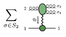
Figure 3: Illustration of eq. 225, which is one possible form of all-orders factorisation of the dispersive part of five-parton amplitudes which (unlike the factorised form in fig. 2) is compatible with the one-loop result eq. 224.

Of course, whether the term ${\mathcal{C}}_{d}$ recieves logarithmic corrections at higher orders, let alone the form they may take, cannot be informed by this one-loop analysis. Much can be learned, therefore, from investigating the NMRK limit two-loop five-gluon amplitudes.

Finally, we turn to the simpler case of a single negative helicity gluon. We obtain the compact results

$$\begin{split}C_{FF}^{(1,\,s)}(p_{2}^{\oplus},p_{3}^{\oplus},p_{4}^{\oplus},q_{2})&=C_{FF}^{(1,\,g)}(p_{2},p_{3},p_{4},q_{2})=-C_{FF}^{(1,\,f)}(p_{2},p_{3},p_{4},q_{2})\\ &=\frac{1}{q_{2\perp}}\left(\frac{q_{2\perp}^{*}}{q_{2\perp}}\right)\frac{X(z-1)^{3}\left(X^{3}{\bar{z}}+X^{2}(z+1){\bar{z}}+Xz(z+1)+z^{2}\right)}{(X+1)^{2}z^{2}({\bar{z}}-1)(X+z)^{2}}\,,\end{split}$$ (226)

$$\begin{split}C_{d}^{(1,\,s)}(p_{2}^{\oplus},p_{3}^{\oplus},p_{4}^{\oplus},q_{2})&=C_{d}^{(1,\,g)}(p_{2},p_{3},p_{4},q_{2})=-C_{d}^{(1,\,f)}(p_{2},p_{3},p_{4},q_{2})\\ &=-\frac{1}{q_{2\perp}}\left(\frac{q_{2\perp}^{*}}{q_{2\perp}}\right)\frac{3X(z-1)^{2}(z-{\bar{z}})}{(X+1)z({\bar{z}}-1)(X+z)}\,.\end{split}$$ (227)

The one-loop amplitude in the NMRK is then

$$\begin{split}&\mathcal{A}^{(1)[-]}_{5}(2^{\oplus},3^{\oplus},4^{\oplus},5^{-\lambda_{1}},1^{\lambda_{1}})\underset{\scriptscriptstyle{\mathrm{NMRK}}}{\to}g_{\mathrm{s}}^{5}\,2s_{12}\,R^{(0)}_{g^{*}}(q_{1})(-F^{d}_{a_{5}a_{1}})C^{(0)}_{g^{*}gg}(-q_{2},p_{5}^{-\lambda_{1}},p_{1}^{\lambda_{1}})\\ &\times\Bigg{\{}\sum_{\sigma\in S_{2}}(F^{a_{\sigma_{3}}}F^{a_{\sigma_{4}}})_{a_{2}c_{2}}\ (N_{c}-N_{f})C_{FF}^{(1,\,s)}(p_{2}^{\oplus},p_{\sigma_{3}}^{\oplus},p_{\sigma_{4}}^{\oplus},q_{2})\,\\ &\quad+\left(d_{A}-2\,d_{F}\right)^{a_{2}a_{3}a_{4}c_{2}}C_{d}^{(1,\,s)}(p_{2}^{\oplus},p_{3}^{\oplus},p_{4}^{\oplus},q_{2})\Bigg{\}}\,.\end{split}$$ (228)

This amplitude is compatible with eq. 28, and we can define the one-loop colour-dressed vertex

$$\begin{split}\mathcal{C}^{(1)}_{ggg^{*}}(p_{2}^{\oplus},p_{3}^{\oplus},p_{4}^{\oplus},q_{2})&=\sum_{\sigma\in S_{2}}(F^{a_{\sigma_{3}}}F^{a_{\sigma_{4}}})_{a_{2}c_{2}}\ (N_{c}-N_{f})C_{FF}^{(1,\,s)}(p_{2}^{\oplus},p_{\sigma_{3}}^{\oplus},p_{\sigma_{4}}^{\oplus},q_{2})\,\\ &\quad+\left(d_{A}-2\,d_{F}\right)^{a_{2}a_{3}a_{4}c_{2}}C_{d}^{(1,\,s)}(p_{2}^{\oplus},p_{3}^{\oplus},p_{4}^{\oplus},q_{2})\,.\end{split}$$ (229)

This colour-dressed vertex has the MRK limit

$$\mathcal{C}^{(1)}_{ggg^{*}}(p_{2}^{\oplus},p_{3}^{\oplus},p_{4}^{\oplus},q_{2})\underset{\scriptscriptstyle{\mathrm{MRK}}}{\to}\mathcal{C}^{(1)}_{ggg^{*}}(p_{2}^{\oplus},p_{3}^{\oplus},q_{1})\mathcal{R}_{g^{*}}^{(0)}(q_{1})\mathcal{V}_{g^{*}gg^{*}}^{(0)}(-q_{1},p_{4}^{\oplus},q_{2}),$$ (230)

as required by the known compatibility of the amplitude with eq. 22.

In the remainder of this paper, we perform an analogous investigation of the one-loop amplitudes with an external quark-antiquark pair.

9 One-loop primitive vertices for the peripheral emission of a quark and gluon

In this section we take the NMRK limit of one-loop primitive amplitudes of three gluons and a quark-antiquark pair. We use the amplitudes provided by ref. Bern:1994fz . Expressions are given in that paper for the following N^-1MHV helicity configurations

$$\{{\bar{q}}^{\ominus},q^{\oplus},g^{\oplus},g^{\oplus},g^{\oplus}\},\quad\{{\bar{q}}^{\ominus},g^{\oplus},q^{\oplus},g^{\oplus},g^{\oplus}\},$$

which in the NMRK limit only give rise to the one-loop $\{g^{\oplus},g^{\oplus},g^{\oplus},g^{*}\}$ vertex discussed in section 7.3.1, and the MHV configurations

$$\{{\bar{q}}^{\ominus},q^{\oplus},g^{\ominus},g^{\oplus},g^{\oplus}\},\quad\{{\bar{q}}^{\ominus},q^{\oplus},g^{\oplus},g^{\ominus},g^{\oplus}\},\quad \{{\bar{q}}^{\ominus},q^{\oplus},g^{\oplus},g^{\oplus},g^{\ominus}\},\quad\{{\bar{q}}^{\ominus},g^{\ominus},q^{\oplus},g^{\oplus},g^{\oplus}\}$$

$$\{{\bar{q}}^{\ominus},g^{\oplus},q^{\oplus},g^{\ominus},g^{\oplus}\},\quad \{{\bar{q}}^{\ominus},g^{\oplus},q^{\oplus},g^{\oplus},g^{\ominus}\}.$$

Let us briefly review how any amplitude can be related to one of the above by discrete transformations. We note that parity conjugation, via complex conjugation, can be used to map to a single-minus or two-minus amplitude, and charge conjugation,

$$A_{n}^{(1,\,m_{L})}(\cdots,i_{q}^{\lambda},\cdots,j_{{\bar{q}}}^{(-\lambda)},\cdots)=A_{n}^{(1,\,m_{R})}(\cdots,i_{{\bar{q}}}^{\lambda},\cdots,j_{q}^{(-\lambda)},\cdots)\,,$$ (231)

can be used to map to an amplitude where the negative-helicity fermion is the antiquark. Cyclicity of the amplitude means the first argument can always be set to be the antiquark. Finally, the reflection identity, eq. 67, can be used to bring the quark into either the second or third entry.

For each configuration, explicit amplitudes are provided in ref. Bern:1994fz for particle content $\mathcal{N}=1_{V}$, $g_{L}$, ${\mathcal{N}=1_{\chi}}_{L}$ and $s_{L}$. We remind the reader that the ${\mathcal{N}=1_{\chi}}_{R}$ and $s_{R}$ amplitudes vanish for these configurations according to eq. 68a and eq. 68b. The fermion contribution can be obtained via the decomposition

$$A_{n}^{(1,\,f_{L})}=A_{n}^{(1,\,{\mathcal{N}=1_{V}}_{L})}-A_{n}^{(1,\,{s}_{L})}\,,$$ (232)

and the $g_{R}$ contribution can be subsequently obtained by means of the supersymmetric decomposition eq. 85, which we duplicate here for the convenience of the reader:

$$A_{n}^{(1,\ \mathcal{N}=1_{V})}=A_{n}^{(1,\,g_{L})}+A_{n}^{(1,\,g_{R})}+A_{n}^{(1,f_{L})}\,.$$ (233)

Following the procedure of section 5.3.2, the left hand side of this equation can be found through the supersymmetric Ward identity

$$a_{5}^{(1,\,\mathcal{N}=1_{V})}(2_{\bar{q}},3_{q},4,5,1)=a_{5}^{(1,\,\mathcal{N}=1_{V})}(2,3,4,5,1)\,.$$ (234)

It follows that

$$c_{{\bar{q}}qgg^{*}}^{(1,\,{\mathcal{N}}=1V)}(p_{2}^{\lambda_{2}},p_{3}^{\lambda_{3}},p_{4}^{\lambda_{4}},q_{2})=c_{gggg^{*}}^{(1,\,{\mathcal{N}}=1V)}(p_{2}^{\lambda_{2}},p_{3}^{\lambda_{3}},p_{4}^{\lambda_{4}},q_{2})\,,$$ (235)

with analogous relations for different orderings of the external particle species. The organisation of this section is similar to section 7, where we first categorise the peripheral-emission vertices by internal particle content, then by helicity configuration, where a minimal set of primitive vertices is given by the three cyclic orderings

$$\{{\bar{q}}^{\ominus},q^{\oplus},g^{\oplus},g^{*}\}\,,\qquad\{{\bar{q}}^{\ominus},g^{\oplus},q^{\oplus},g^{*}\}\,,\qquad\{g^{\oplus},{\bar{q}}^{\ominus},q^{\oplus},g^{*}\}\,.$$

9.1 $\mathcal{N}=4$ contribution

Although in practice we use a $\mathcal{N}=1_{V}$ multiplet decomposition, eq. 233, to organise the amplitudes and vertices, it is worthwhile to analyse the amplitudes with a circulating $\mathcal{N}=4$ multiplet for two reasons. Firstly, ref. Bern:1994fz writes the $g_{L}$ and $\mathcal{N}=1_{V}$ amplitudes in terms of the function eq. 161, and this proves convenient also for the factorised expressions. Secondly, it provides us with the simplest context to study the key difference between the pure-gluon case and the case with an external quark-antiquark pair.

Recall the discussion of eq. 161 in section 7.1.1. To be concrete, let us study the physical scattering

$$q(p_{2})\,g(p_{1})\to q(p_{3})\,g(p_{4})\,g(p_{5}).$$

The treatment of the ordering $\{p_{2},p_{3},p_{4},q_{2}\}$ proceeds similarly to the pure gluon case, and by a SUSY Ward identity we obtain

$$\begin{split}\mathrm{Re}\left[a_{5}^{(1,\,\mathcal{N}=4)}(2_{\bar{q}},3_{g},4,5,1)\right]\underset{\scriptscriptstyle{\mathrm{NMRK}}}{\to}&c_{{\bar{q}}qgg^{*}}^{(1,\,\mathcal{N}=4)}(p_{2},p_{3},p_{4},q_{2})\\ +&r_{g^{*}}^{(1,\,\mathcal{N}=4)}(q_{2};p_{4}^{+}p_{5}^{-})+c_{g^{*}gg}^{(1,\,\mathcal{N}=4)}(-q_{2},p_{5},p_{1})\end{split}$$ (236)

with primitive vertex

$$\begin{split}c_{{\bar{q}}qgg^{*}}^{(1,\,\mathcal{N}=4)}(p_{2},p_{3},p_{4},q_{2})=&c_{ggg^{*}}^{(1,\,\mathcal{N}=4)}(p_{2},p_{3},q_{1})+r_{g^{*}}^{(1,\,\mathcal{N}=4)}(q_{1};s_{34})\\ +&v^{(1,\,\mathcal{N}=4)}(t_{1},\frac{s_{34}\,p_{4}^{+}}{(p_{3}^{+}+p_{4}^{+})},t_{2})\,.\end{split}$$ (237)

Likewise, for the second colour-ordering in eq. 159 we write

$$\begin{split}\mathrm{Re}\left[a_{5}^{(1,\,\mathcal{N}=4)}(4,2_{\bar{q}},3_{q},5,1)\right]\underset{\scriptscriptstyle{\mathrm{NMRK}}}{\to}&c_{g{\bar{q}}qg^{*}}^{(1,\,\mathcal{N}=4)}(p_{4},p_{2},p_{3},q_{2})\\ +&r_{g^{*}}^{(1,\,\mathcal{N}=4)}(q_{2};p_{4}^{+}p_{5}^{-})+c_{g^{*}gg}^{(1,\,\mathcal{N}=4)}(-q_{2},p_{5},p_{1})\,,\end{split}$$ (238)

with primitive vertex

$$\begin{split}c_{g{\bar{q}}qg^{*}}^{(1,\,\mathcal{N}=4)}(p_{4},p_{2},p_{3},q_{2})=&c_{ggg^{*}}^{(1,\,\mathcal{N}=4)}(p_{3},p_{2},q_{1})+r_{g^{*}}^{(1,\,\mathcal{N}=4)}(q_{1};s_{24})\\ +&v^{(1,\,\mathcal{N}=4)}(t_{1},\frac{s_{24}\,p_{4}^{+}}{(p_{2}^{+}+p_{4}^{+})},t_{2})\,.\end{split}$$ (239)

In this form, it is transparent that the correct large logarithms are generated by the ${\bar{q}}qgg^{*}$ and $g{\bar{q}}qg^{*}$ vertices in the MRK limit. This follows from the $U(1)$-decoupling identities, e.g.

$$C^{(0)}_{{\bar{q}}qgg^{*}}(p_{2}^{\oplus},p_{3}^{\ominus},p_{4}^{\oplus},q_{2})+C^{(0)}_{{\bar{q}}gqg^{*}}(p_{2}^{\oplus},p_{4}^{\oplus},p_{3}^{\ominus},q_{2})+C^{(0)}_{g{\bar{q}}qg^{*}}(p_{4}^{\oplus},p_{2}^{\oplus},p_{3}^{\ominus},q_{2})=0\,,$$ (240)

which in the MRK limit becomes

$$C^{(0)}_{{\bar{q}}qgg^{*}}(p_{2}^{\oplus},p_{3}^{\ominus},p_{4}^{\oplus},q_{2})=-C^{(0)}_{g{\bar{q}}qg^{*}}(p_{4}^{\oplus},p_{2}^{\oplus},p_{3}^{\ominus},q_{2})\,,$$ (241)

due to the power-suppression of the second term in eq. 240. The one-loop corrections, eqs. 237 and 239 on the other hand become equal in the MRK limit, due to the limiting behaviour

$$\frac{s_{24}\,p_{4}^{+}}{(p_{2}^{+}+p_{4}^{+})}\underset{{\mathrm{MRK}}}{=}\frac{s_{34}\,p_{4}^{+}}{(p_{3}^{+}+p_{4}^{+})}\,.$$ (242)

Thus the kinematic coefficients of the first two colour-structures in eq. 159 are equal and opposite, as required by compatibility with eq. 22.

We also need to consider the $\delta\Delta$ coefficient, eq. 160. This must be free from large logarithms in the NMRK and must vanish in the MRK limit. To verify the former condition, we can write, (merely for convenience to separate out a large logarithmic term and a backward $g^{*}gg$ vertex)

$$\begin{split}\mathrm{Re}\left[a_{5}^{(1,\,\mathcal{N}=4)}(2_{\bar{q}},4,3_{q},5,1)\right]\underset{\scriptscriptstyle{\mathrm{NMRK}}}{\to}&c_{{\bar{q}}gqg^{*}}^{(1,\,\mathcal{N}=4)}(p_{2},p_{4},p_{3},q_{2})\\ +&r_{g^{*}}^{(1,\,\mathcal{N}=4)}(q_{2};p_{3}^{+}p_{5}^{-})+c_{g^{*}gg}^{(1,\,\mathcal{N}=4)}(-q_{2},p_{5},p_{1})\,,\end{split}$$ (243)

with vertex

$$\begin{split}c_{{\bar{q}}gqg^{*}}^{(1,\,\mathcal{N}=4)}(p_{2},p_{4},p_{3},q_{2})=&c_{ggg^{*}}^{(1,\,\mathcal{N}=4)}(p_{2},p_{4},q_{1}^{\prime})+r_{g^{*}}^{(1,\,\mathcal{N}=4)}(q_{1}^{\prime};s_{43})\\ +&v^{(1,\,\mathcal{N}=4)}(t_{1}^{\prime},\frac{s_{43}\,p_{3}^{+}}{(p_{4}^{+}+p_{3}^{+})},t_{2})\,.\end{split}$$ (244)

All large logarithmic behaviour in the $m{=}g$ amplitudes can be conveniently written in terms of the $\mathcal{N}=4$ function eq. 161, and only the $m{=}g_{L}$ amplitudes have large logarithms in the NMRK limit. Therefore the LL behaviour of eq. 160 in the NMRK limit coincides with

$$\begin{split}{\mathrm{Disp}\left[{A^{(1,\,\mathcal{N}=4)}_{\delta\Delta}(p_{2},p_{3},p_{4},p_{5},p_{1})}\right]}\underset{\scriptscriptstyle{\mathrm{NMRK}}}{\to}&C^{(0)}_{{\bar{q}}qgg^{*}}(p_{2},p_{3},p_{4},q_{2})\bigg{(}c^{(1,\,\mathcal{N}=4)}_{{\bar{q}}qgg^{*}}(p_{2},p_{3},p_{4},q_{2})\\ &-c^{(1,\,\mathcal{N}=4)}_{{\bar{q}}gqg^{*}}(p_{2},p_{4},p_{3},q_{2})+r^{(1,\,g)}_{g^{*}}(q_{2},p_{4}^{+}p_{5}^{-})-r^{(1,\,g)}_{g^{*}}(q_{2},p_{3}^{+}p_{5}^{-})\bigg{)}\\ +&C^{(0)}_{g{\bar{q}}qg^{*}}(p_{4},p_{2},p_{3},q_{2})\bigg{(}c^{(1,\,\mathcal{N}=4)}_{g{\bar{q}}qg^{*}}(p_{4},p_{2},p_{3},q_{2})\\ &-c^{(1,\,\mathcal{N}=4)}_{{\bar{q}}gqg^{*}}(p_{2},p_{4},p_{3},q_{2})+r^{(1,\,g)}_{g^{*}}(q_{2},p_{4}^{+}p_{5}^{-})-r^{(1,\,g)}_{g^{*}}(q_{2},p_{3}^{+}p_{5}^{-})\bigg{)}\,.\end{split}$$ (245)

We note that all dependence on the backward $g^{*}ggg$ vertex cancels, so that this partial amplitude only contributes to the forward physics, from which we define the partial vertex

$$C^{(1,\,\mathcal{N}=4)}_{\delta\Delta}(p_{2},p_{3},p_{4},q_{2})\equiv\left.{\mathrm{Disp}\left[{A^{(1,\,\mathcal{N}=4)}_{\delta\Delta}(p_{2},p_{3},p_{4},p_{5},p_{1})}\right]}\right|_{\mathrm{NMRK}}\,.$$

We note that this partial vertex is free from large logarithms, because the difference of Reggeisation factors

$$r^{(1,\,g)}_{g^{*}}(q_{2},p_{4}^{+}p_{5}^{-})-r^{(1,\,g)}_{g^{*}}(q_{2},p_{3}^{+}p_{5}^{-})\,,$$

depends only on the ratio $X=p_{3}^{+}/p_{4}^{+}$ which is finite in the NMRK limit. Finally, we note that due to eq. 241 and eq. 242, the entire partial vertex vanishes in the MRK limit as expected.

9.2 $\mathcal{N}=1_{\chi}$ contribution

In this section, we repeat the analysis of section 7.2 but for amplitudes with an external quark-antiquark pair.

9.2.1 $\{{\bar{q}}^{\ominus},q^{\oplus},g^{\oplus},g^{*}\}$

The relevant amplitudes have a very simple NMRK limit, e.g.

$$\begin{split}a_{5}^{(1,\ {\mathcal{N}=1_{\chi}}_{L})}(2_{\bar{q}}^{\ominus},3_{q}^{\oplus},4^{\oplus},5^{\ominus},1^{\oplus})\underset{\scriptscriptstyle{\mathrm{NMRK}}}{\to}&-\frac{(X+z)}{X(z-1)}L_{0}\left(\frac{-s_{23}}{-s_{51}}\right)\,.\end{split}$$ (246)

To obtain the ${\bar{q}}qgg^{*}$ vertex we use eq. 132 to add and subtract

$$c^{(1,\ \mathcal{N}=1_{\chi})}_{{\bar{q}}qg^{*}}(p_{2}^{\ominus},p_{3}^{\oplus},q_{1})+c_{g^{*}gg}^{(1,\ \mathcal{N}=1_{\chi})}(-q_{2},p_{5}^{\ominus},p_{1}^{\oplus})=\frac{1}{2}\log\left(\frac{-s_{23}}{-s_{51}}\right)\,,$$ (247)

leading to

$$\begin{split}a_{5}^{(1,\,{\mathcal{N}=1_{\chi}}_{L})}(2_{\bar{q}}^{\ominus},3_{q}^{\oplus},4^{\oplus},5^{\ominus},1^{\oplus})\underset{\scriptscriptstyle{\mathrm{NMRK}}}{\to}&c^{(1,\,\mathcal{N}=1_{\chi})}_{{\bar{q}}qg^{*}}(p_{2}^{\ominus},p_{3}^{\oplus},q_{1})\\ +&\frac{X(1+z-{\bar{z}})-z({\bar{z}}-2)}{2X|z-1|^{2}}L_{0}\left(\frac{-s_{23}}{-s_{51}}\right)\\ +&c_{g^{*}gg}^{(1,\,\mathcal{N}=1_{\chi})}(-q_{2},p_{5}^{\ominus},p_{1}^{\oplus})\,.\end{split}$$ (248)

We thus define the 2-parton peripheral-emission vertex to be

$$\begin{split}c^{(1,\,\mathcal{N}=1_{\chi})}_{{\bar{q}}qgg^{*}}(p_{2}^{\ominus},p_{3}^{\oplus},p_{4}^{\oplus},q_{2})=&c^{(1,\,\mathcal{N}=1_{\chi})}_{{\bar{q}}qg^{*}}(p_{2}^{\ominus},p_{3}^{\oplus},q_{1})+\frac{X(1+z-{\bar{z}})-z({\bar{z}}-2)}{2X|z-1|^{2}}L_{0}\left(\frac{-t_{1}}{-t_{2}}\right)\,,\end{split}$$ (249)

which has the trivial MRK limit

$$\begin{split}c^{(1,\,\mathcal{N}=1_{\chi})}_{{\bar{q}}qgg^{*}}(p_{2}^{\ominus},p_{3}^{\oplus},p_{4}^{\oplus},q_{2})\underset{X\to\infty}{\to}&c^{(1,\,\mathcal{N}=1_{\chi})}(2_{\bar{q}}^{\ominus},3_{q}^{\oplus},q_{1})+v_{g^{*}gg^{*}}^{(1,\,\mathcal{N}=1_{\chi})}(-q_{1},p_{4},q_{2})\,.\end{split}$$ (250)

9.2.2 $\{{\bar{q}}^{\ominus},g^{\oplus},q^{\oplus},g^{*}\}$

The amplitudes which would give rise to this vertex do not contribute to eq. 159. Furthermore, these amplitudes are zero:

$$A_{5}^{(1,\,{\mathcal{N}=1_{\chi}}_{L})}({\bar{q}}^{\ominus},g^{\oplus},q^{\oplus},g^{\oplus},g^{\ominus})=A_{5}^{(1,\,{\mathcal{N}=1_{\chi}}_{L})}({\bar{q}}^{\ominus},g^{\oplus},q^{\oplus},g^{\ominus},g^{\oplus})=0\,.$$ (251)

Following the discussion in section 5.3.2, we can nevertheless define

$$c_{{\bar{q}}qgg^{*}}^{(1,\,{\mathcal{N}=1_{\chi}}_{L})}(p_{2}^{\ominus},p_{3}^{\oplus},p_{4}^{\oplus},q_{2})=-c_{g^{*}gg}^{(1,\,{\mathcal{N}=1_{\chi}})}(-q_{2},p_{5}^{\lambda_{5}},p_{1}^{\lambda_{1}})\,,$$ (252)

which only depends on the invariant $s_{51}=s_{234}$.

9.2.3 $\{g^{\oplus},{\bar{q}}^{\ominus},q^{\oplus},g^{*}\}$

As in section 9.2.1, the NMRK limits of the relevant amplitudes are again very simple, for example

$$\begin{split}a_{5L}^{(1,\ \mathcal{N}=1_{\chi})}(2_{\bar{q}}^{\ominus},3_{q}^{\oplus},5^{\ominus},1^{\oplus},4^{\oplus})\underset{\scriptscriptstyle{\mathrm{NMRK}}}{\to}&\frac{1}{(z-1)}L_{0}\left(\frac{-s_{23}}{-s_{51}}\right)\,.\end{split}$$ (253)

We remark that this is simply $X/(X+z)$ times the amplitude in eq. 246. Recalling the NMRK behaviour of the tree level amplitudes,

$$\frac{A^{(0)}(4^{\oplus},2_{\bar{q}}^{\ominus},3_{q}^{\oplus},5^{\ominus},1^{\oplus})}{A^{(0)}(2_{\bar{q}}^{\ominus},3_{q}^{\oplus},4^{\oplus},5^{\ominus},1^{\oplus})}\underset{\scriptscriptstyle{\mathrm{NMRK}}}{\to}\frac{X}{X+z}$$ (254)

we see that

$$A^{(1,\ \mathcal{N}=1_{\chi})}(4^{\oplus},2_{\bar{q}}^{\ominus},3_{q}^{\oplus},5^{\ominus},1^{\oplus})+A^{(1,\ \mathcal{N}=1_{\chi})}(2_{\bar{q}}^{\ominus},3_{q}^{\oplus},4^{\oplus},5^{\ominus},1^{\oplus})\underset{\scriptscriptstyle{\mathrm{NMRK}}}{\to}0\,,$$ (255)

which is reminiscent of the identity eq. 78, which followed from Furry’s theorem, but for an off-shell gluon with momentum $p_{5}+p_{1}$.

The vertex resulting from eq. 253 is

$$\begin{split}c^{(1,\,\mathcal{N}=1_{\chi})}_{{\bar{q}}qgg^{*}}(p_{4}^{\oplus},p_{2}^{\ominus},p_{3}^{\oplus},q_{2})=&c^{(1,\,\mathcal{N}=1_{\chi})}_{{\bar{q}}qg^{*}}(p_{2}^{\ominus},p_{3}^{\oplus},q_{1})+\frac{X(1+z-{\bar{z}})+|z|^{2}}{2X|z-1|^{2}}L_{0}\left(\frac{-t_{1}}{-t_{2}}\right)\,,\end{split}$$ (256)

which has the transparent MRK limit

$$\begin{split}c^{(1,\,\mathcal{N}=1_{\chi})}_{{\bar{q}}qgg^{*}}(p_{4}^{\oplus},p_{2}^{\ominus},p_{3}^{\oplus},q_{2})\underset{X\to\infty}{\to}&c^{(1,\,\mathcal{N}=1_{\chi})}(2_{\bar{q}}^{\ominus},3_{q}^{\oplus},q_{1})+v_{g^{*}gg^{*}}^{(1,\,\mathcal{N}=1_{\chi})}(-q_{1},p_{4},q_{2})\,.\end{split}$$ (257)

9.3 Complex scalar contribution

The procedure to obtain these vertices proceeds similarly to section 9.2 and we simply collect the primitive vertices here. The ${\bar{q}}^{\ominus}q^{\ominus}g^{\oplus}g^{*}$ vertex is

$$\begin{split}c_{{\bar{q}}qgg^{*}}^{(1,\ s_{L})}(p_{2}^{\ominus},p_{3}^{\oplus},p_{4}^{\oplus},q_{2})&=c_{{\bar{q}}qg^{*}}^{(1,\ s_{L})}(p_{2},p_{3},q_{2})+\frac{1}{6}\frac{X(1+z-{\bar{z}})-z({\bar{z}}-2)}{X|z-1|^{2}}L_{0}\left(\frac{-t_{1}}{-t_{2}}\right)\\ &+\frac{1}{3}\frac{z|X+z|^{2}(X(1+z-{\bar{z}})+|z|^{2})}{X^{3}(z-1)^{3}({\bar{z}}-1)^{2}}L_{2}\left(\frac{-t_{1}}{-t_{2}}\right)-\frac{|X+z|^{2}}{6X(1+X)(z-1){\bar{z}}}\,.\end{split}$$ (258)

The ${\bar{q}}^{\ominus}g^{\oplus}q^{\ominus}g^{*}$ vertex is

$$c_{{\bar{q}}gqg^{*}}^{(1,\,s_{L})}(p_{2}^{\ominus},p_{4}^{\oplus},p_{3}^{\oplus},q_{2})=-c_{g^{*}gg}^{(1,\,{s})}(-q_{2},p_{5}^{\lambda_{5}},p_{1}^{\lambda_{1}})\,.$$ (259)

Finally, the $g^{\oplus}{\bar{q}}^{\ominus}q^{\ominus}g^{*}$ vertex is

$$\begin{split}c_{g{\bar{q}}qg^{*}}^{(1,\ s_{L})}(p_{4}^{\oplus},p_{2}^{\ominus},p_{3}^{\oplus},q_{2})&=c_{{\bar{q}}qg^{*}}^{(1,\ s_{L})}(p_{2},p_{3},q_{2})+\frac{1}{6}\frac{X(1+z-{\bar{z}})+|z|^{2}}{X|z-1|^{2}}L_{0}\left(\frac{-t_{1}}{-t_{2}}\right)\\ &+\frac{1}{3}\frac{z(X+{\bar{z}})^{2}(X(1+z-{\bar{z}})+|z|^{2})}{X^{3}(z-1)^{3}({\bar{z}}-1)^{2}}L_{2}\left(\frac{-t_{1}}{-t_{2}}\right)-\frac{(X+{\bar{z}})^{2}}{6X(1+X)(z-1){\bar{z}}}\,.\end{split}$$ (260)

9.4 Gluon contribution

Again, the analysis proceeds similarly to section 9.2 and we simply collect the $g_{L}$ primitive vertices here. The $g_{R}$ vertices can be obtained via the supersymmetric decomposition eq. 85. The ${\bar{q}}^{\ominus}q^{\oplus}g^{\oplus}g^{*}$ vertex is

$$\begin{split}c_{{\bar{q}}qgg^{*}}^{(1,\ g_{L})}(p_{2}^{\ominus},p_{3}^{\oplus},p_{4}^{\oplus},q_{2})&=c_{{\bar{q}}qg^{*}}^{(1,\ g_{L})}(p_{2},p_{3},q_{1})+r_{g^{*}}^{(1,\ g)}(t_{1};s_{34})+v^{(1,\,\mathcal{N}=4)}\left(t_{1},\frac{s_{34}\,p_{4}^{+}}{(p_{3}^{+}+p_{4}^{+})},t_{2}\right)\\ &+\left(c_{{\bar{q}}qgg^{*}}^{(1,\,s_{L})}(p_{2},p_{3},p_{4},q_{2})-c_{{\bar{q}}qg^{*}}^{(1,\,s_{L})}(p_{2},p_{3},q_{1})\right)\\ &-4\frac{X(1+z-{\bar{z}})+z}{2X|z-1|^{2}}L_{0}\left(\frac{-t_{1}}{-t_{2}}\right)\\ &-\frac{z}{X}L_{s_{-1}}\left(\frac{-t_{1}}{-t_{2}},\frac{-t_{1}^{\prime}}{-t_{2}}\right)-\frac{z}{2X(z-1)^{2}}L_{1}\left(\frac{-t_{1}}{-t_{2}}\right)\,.\end{split}$$ (261)

The ${\bar{q}}^{\ominus}g^{\oplus}q^{\oplus}g^{*}$ vertex is

$$\begin{split}c_{{\bar{q}}gqg^{*}}^{(1,\ g_{L})}(p_{2}^{\ominus},p_{4}^{\oplus},p_{3}^{\oplus},q_{2})=&c_{{\bar{q}}gqg^{*}}^{(1,\ \mathcal{N}=4)}(p_{2},p_{4},p_{3},q_{1})+\frac{1}{\epsilon^{2}}\left(\frac{\mu^{2}}{-s_{24}}\right)^{\epsilon}+\frac{1}{\epsilon^{2}}\left(\frac{\mu^{2}}{-s_{34}}\right)^{\epsilon}-\frac{3}{2}\left(\frac{\mu^{2}}{-s_{24}}\right)\\ &+L_{s_{-1}}\left(\frac{-s_{24}}{-t_{2}},\frac{-s_{34}}{-t_{2}}\right)-\frac{2z}{z-1}L_{0}\left(\frac{-s_{24}}{-t_{2}}\right)+\frac{z^{2}}{2(z-1)^{2}}L_{1}\left(\frac{-s_{24}}{-t_{2}}\right)-3\,,\end{split}$$ (262)

with $\mathcal{N}=4$ vertex as in eq. 244. Recalling the comment beneath eq. 194, we emphasise that only the dispersive part of eq. 262 for the physical scattering $q(p_{2})\to q(p_{3})g(p_{4})$ should be taken. Finally, the $g^{\oplus}{\bar{q}}^{\ominus}q^{\oplus}g^{*}$ vertex is

$$\begin{split}&c_{g{\bar{q}}qg^{*}}^{(1,\ g_{L})}(p_{4}^{\oplus},p_{2}^{\ominus},p_{3}^{\oplus},q_{2})=c_{{\bar{q}}qg^{*}}^{(1,\ g_{L})}(p_{2},p_{3},q_{1})+r_{g^{*}}^{(1,\ g)}(t_{1};s_{24})+v^{(1,\,\mathcal{N}=4)}\left(t_{1},\frac{-s_{24}\,p_{4}^{+}}{(p_{3}^{+}+p_{4}^{+})},t_{2}\right)\\ &+(c_{g{\bar{q}}qg^{*}}^{(1,\ s_{L})}(p_{4},p_{2},p_{3},q_{2})-c_{{\bar{q}}qg^{*}}^{(1,\ s_{L})}(p_{2},p_{3},q_{1}))\\ &+\left(\frac{X(z+{\bar{z}}-1)-2z(X+{\bar{z}})+4X({\bar{z}}-1)+|z|^{2}}{2X|z-1|^{2}}-\frac{z(2X+z)(X+{\bar{z}})}{|z-1|^{2}(X+z)^{2}}\right)L_{0}\left(\frac{-t_{1}}{-t_{2}}\right)\\ &+\left(\frac{X^{2}\left(({\bar{z}}-1)^{2}-z^{2}\right)+Xz\left(-2(z+1){\bar{z}}+{\bar{z}}^{2}+1\right)-z^{2}{\bar{z}}^{2}}{2X(z-1)^{2}({\bar{z}}-1)^{2}(X+z)}\right)L_{1}\left(\frac{-t_{1}}{-t_{2}}\right)\\ &+\left(-\frac{Xz^{2}}{(X+z)^{3}}+\frac{2Xz}{(X+z)^{2}}+\frac{z}{X+z}\right)L_{s_{-1}}\left(\frac{-t_{1}}{-t_{2}},\frac{-t_{1}^{\prime}}{-t_{2}}\right)\\ &-\left(\frac{z(X+{\bar{z}})\left(-5X^{2}+Xz(4{\bar{z}}-7)-5X{\bar{z}}+2z^{2}({\bar{z}}-1)-3z{\bar{z}}\right)}{2(z-1)^{2}({\bar{z}}-1)^{2}(X+z)^{2}}\right)L_{1}\left(\frac{-t_{1}^{\prime}}{-t_{2}}\right)\\ &+\frac{X^{2}(4z+{\bar{z}}-1)+2Xz(z+3{\bar{z}}-1)+z^{2}(3{\bar{z}}-1)}{2(z-1)({\bar{z}}-1)(X+z)^{2}}\,.\end{split}$$ (263)

10 Colour-dressed one-loop vertex for the peripheral emission of a quark and gluon

In section 6 we analysed the colour structure of the one-loop ${\bar{q}}qggg$ amplitudes at leading power in the NMRK limit. In the previous section we analysed the factorisation properties of the primitive amplitudes in the NMRK limit. Following the procedure of section 8, we now assemble the NMRK limit of the colour-dressed amplitude.

As in section 8, it is useful to consider colour-dressed vertices for each of the colour structures in eq. 159. For the tree-level colour structures we define

$${\mathcal{C}}_{TT}(p_{2},p_{3},p_{4},q_{2})={\mathcal{C}}^{(0)}_{TT}(p_{2},p_{3},p_{4},q_{2})+{\mathcal{C}}_{TT}^{(1)}(p_{2},p_{3},p_{4},q_{2})+\mathcal{O}(g_{\mathrm{s}}^{6})\,,$$ (264)

where the tree-level terms are taken from eq. 45,

$${\mathcal{C}}^{(0)}_{TT}(p_{2},p_{3},p_{4},q_{2}) =g_{\mathrm{s}}^{2}(T^{a_{4}}T^{c_{2}})_{\imath_{3}\bar{\imath}_{2}}\ C^{(0)}_{{\bar{q}}qgg^{*}}(p_{2}^{\lambda_{2}},p_{3}^{\lambda_{3}},p_{4}^{\lambda_{4}},q_{2})$$ (265)

$${\mathcal{C}}^{(0)}_{TT}(p_{4},p_{2},p_{3},q_{2}) =g_{\mathrm{s}}^{2}(T^{c_{2}}T^{a_{4}})_{\imath_{3}\bar{\imath}_{2}}\ C^{(0)}_{{\bar{q}}qgg^{*}}(p_{4}^{\lambda_{4}},p_{2}^{\lambda_{2}},p_{3}^{\lambda_{3}},q_{2})$$ (266)

such that

$$\begin{split}\mathcal{C}^{(0)}_{{\bar{q}}qgg^{*}}(p_{2}^{\lambda_{2}},p_{3}^{\lambda_{3}},p_{4}^{\lambda_{4}},q_{2})={\mathcal{C}}^{(0)}_{TT}(p_{2},p_{3},p_{4},q_{2})+{\mathcal{C}}^{(0)}_{TT}(p_{4},p_{2},p_{3},q_{2})\,.\end{split}$$ (267)

The NMRK limit of the one-loop amplitudes lead us to define the one-loop correction to these colour-dressed vertices,

$$\begin{split}&\mathcal{C}^{(1)}_{TT}(p_{2},p_{3},p_{4},q_{2})=c_{\Gamma}g_{s}^{4}\big{(}T^{a_{4}}T^{d}\big{)}_{\imath_{3}\bar{\imath}_{2}}C^{(0)}_{{\bar{q}}qgg^{*}}(p_{2},p_{3},p_{4},q_{2})\\ &\ \times\left(N_{c}\,c^{(1,\,g_{L})}_{{\bar{q}}qgg^{*}}(p_{2},p_{3},p_{4},q_{2})-\frac{1}{N_{c}}\,c^{(1,\,g_{R})}_{{\bar{q}}qgg^{*}}(p_{2},p_{3},p_{4},q_{2})+N_{f}\,c^{(1,\,f_{L})}_{{\bar{q}}qgg^{*}}(p_{2},p_{3},p_{4},q_{2})\right)\,,\end{split}$$ (268)

$$\begin{split}&\mathcal{C}^{(1)}_{TT}(p_{4},p_{2},p_{3},q_{2})=c_{\Gamma}g_{s}^{4}\big{(}T^{d}T^{a_{4}}\big{)}_{\imath_{3}\bar{\imath}_{2}}C^{(0)}_{{\bar{q}}qgg^{*}}(p_{4},p_{2},p_{3},q_{2})\\ &\ \times\left(N_{c}\,c^{(1,\,g_{L})}_{{\bar{q}}qgg^{*}}(p_{4},p_{2},p_{3},q_{2})-\frac{1}{N_{c}}\,c^{(1,\,g_{R})}_{{\bar{q}}qgg^{*}}(p_{4},p_{2},p_{3},q_{2})+N_{f}\,c^{(1,\,f_{L})}_{{\bar{q}}qgg^{*}}(p_{4},p_{2},p_{3},q_{2})\right)\,.\end{split}$$ (269)

Similarly we define a colour-dressed vertex for the new colour structure which first appears at one loop,

$$\mathcal{C}^{(1)}_{\delta\Delta}(p_{2},p_{3},p_{4},q_{2})=\mathcal{C}^{(1)}_{\delta\Delta}(p_{2},p_{3},p_{4},q_{2})+{\mathcal{O}}(g_{\mathrm{s}}^{4})\,.$$ (270)

As in section 9.1, the partial amplitude eq. 160 for $m{\in}\{g_{L},g_{R}\}$ only contributes to the forward vertex and we find

$$\begin{split}\mathcal{C}^{(1)}_{\delta\Delta}(p_{2},p_{3},p_{4},q_{2})=c_{\Gamma}g_{s}^{4}\,\delta_{\imath_{3}\bar{\imath}_{2}}\Delta_{da_{4}}\,\Big{(}C^{(1,\,g_{L})}_{\delta\Delta}(p_{2},p_{3},p_{4},q_{2})+C^{(1,\,g_{R})}_{\delta\Delta}(p_{2},p_{3},p_{4},q_{2})\Big{)}\,,\end{split}$$ (271)

with

$$\begin{split}C^{(1,\,g_{L})}_{\delta\Delta}(p_{2},p_{3},p_{4},q_{2})=&C^{(0)}_{{\bar{q}}qgg^{*}}(p_{2},p_{3},p_{4},q_{2})\bigg{(}c^{L(1,\,g)}_{{\bar{q}}qgg^{*}}(p_{2},p_{3},p_{4},q_{2})-c^{L(1,\,g)}_{{\bar{q}}gqg^{*}}(p_{2},p_{4},p_{3},q_{2})\\ &\hskip 120.00018pt+r^{(1,\,g)}_{g^{*}}(q_{2},p_{4}^{+}p_{5}^{-})-r^{(1,\,g)}_{g^{*}}(q_{2},p_{3}^{+}p_{5}^{-})\bigg{)}\\ +&C^{(0)}_{g{\bar{q}}qg^{*}}(p_{4},p_{2},p_{3},q_{2})\bigg{(}c^{L(1,\,g)}_{g{\bar{q}}qg^{*}}(p_{4},p_{2},p_{3},q_{2})-c^{L(1,\,g)}_{{\bar{q}}gqg^{*}}(p_{2},p_{4},p_{3},q_{2})\\ &\hskip 120.00018pt+r^{(1,\,g)}_{g^{*}}(q_{2},p_{4}^{+}p_{5}^{-})-r^{(1,\,g)}_{g^{*}}(q_{2},p_{3}^{+}p_{5}^{-})\bigg{)}\,,\end{split}$$ (272)

and

$$\begin{split}C^{(1,\,g_{R})}_{\delta\Delta}(p_{2},p_{3},p_{4},q_{2})=&C^{(0)}_{{\bar{q}}qgg^{*}}(p_{2},p_{3},p_{4},q_{2})\bigg{(}c^{(1,\,g_{R})}_{{\bar{q}}qgg^{*}}(p_{2},p_{3},p_{4},q_{2})-c^{(1,\,g_{R})}_{{\bar{q}}gqg^{*}}(p_{2},p_{4},p_{3},q_{2})\bigg{)}\\ +&C^{(0)}_{g{\bar{q}}qg^{*}}(p_{4},p_{2},p_{3},q_{2})\bigg{(}c^{(1,\,g_{R})}_{g{\bar{q}}qg^{*}}(p_{4},p_{2},p_{3},q_{2})-c^{(1,\,g_{R})}_{{\bar{q}}gqg^{*}}(p_{2},p_{4},p_{3},q_{2})\bigg{)}\,.\end{split}$$ (273)

As in eq. 245, eq. 272 is free from large logarithms. With these definitions we can write the NMRK limit of the one-loop amplitudes in the compact form

$$\begin{split}&\frac{1}{2s}{\mathrm{Disp}\left[{\mathcal{A}_{5}^{(1)[-]}\left(\bar{q}_{2},q_{3},g_{4},g_{5},g_{1}\right)}\right]}\\ &\underset{\scriptscriptstyle{\mathrm{NMRK}}}{\to}\bigg{(}\mathcal{C}^{(1)}_{TT}(p_{2},p_{3},p_{4},q_{2})+\mathcal{C}^{(1)}_{TT}(p_{4},p_{2},p_{3},q_{2})+\mathcal{C}^{(1)}_{\delta\Delta}(p_{2},p_{3},p_{4},q_{2})\bigg{)}\mathcal{R}^{(0)}_{g^{*}}(q_{2})\mathcal{C}^{(0)}_{g^{*}gg}(-q_{2},p_{5},p_{1})\\ &\quad\ +\bigg{(}\mathcal{C}^{(0)}_{TT}(p_{2},p_{3},p_{4},q_{2})+\mathcal{C}^{(0)}_{TT}(p_{4},p_{2},p_{3},q_{2})\bigg{)}\mathcal{R}^{(1)}_{g^{*}}(q_{2};p_{4}^{+}p_{5}^{-})\mathcal{C}^{(0)}_{g^{*}gg}(-q_{2},p_{5},p_{1})\\ &\quad\ +\bigg{(}\mathcal{C}^{(0)}_{TT}(p_{2},p_{3},p_{4},q_{2})+\mathcal{C}^{(0)}_{TT}(p_{4},p_{2},p_{3},q_{2})\bigg{)}\mathcal{R}^{(0)}_{g^{*}}(q_{2})\mathcal{C}^{(1)}_{g^{*}gg}(-q_{2},p_{5},p_{1})\,.\end{split}$$ (274)

Unlike the pure-gluon case, eq. 217, eq. 274 is compatible with an all-orders factorisation of the form

$$\begin{split}{\mathrm{Disp}\left[{\mathcal{A}_{5}^{(1)[-]}\left(\bar{q}_{2},q_{3},g_{4},f_{5},f_{1}\right)}\right]}\underset{\scriptscriptstyle{\mathrm{NMRK}}}{\to}&2s\,\mathcal{C}_{\bar{q}qgg^{*}}(p_{2},p_{3},p_{4},q_{2})\mathcal{R}_{g^{*}}(q_{2};p_{4}^{+}p_{5}^{-})\mathcal{C}_{g^{*}f_{5}f_{1}}(-q_{2},p_{5},p_{1})\,,\end{split}$$ (275)

where the one-loop correction to eq. 45 is simply given by the sum of the three colour-dressed vertices

$$\begin{split}C^{(1)}_{\bar{q}qgg^{*}}(p_{2},p_{3},p_{4},q_{2})=\mathcal{C}^{(1)}_{TT}(p_{2},p_{3},p_{4},q_{2})+\mathcal{C}^{(1)}_{TT}(p_{4},p_{2},p_{3},q_{2})+\mathcal{C}^{(1)}_{\delta\Delta}(p_{2},p_{3},p_{4},q_{2})\,.\end{split}$$ (276)

11 Conclusions

In this paper we have analysed the dispersive parts of the one-loop $ggggg$ and ${\bar{q}}qggg$ ampltiudes in the NMRK limit eq. 294. The final results are presented in a compact notation in eq. 224 and eq. 274 respectively. In both cases, to leading power, the amplitudes comprise solely of the exchange of a colour octet in the $t_{2}$ channel. Equation 274 is compatible with an all-orders factorisation of the form eq. 28, which defines the colour dressed one-loop ${\bar{q}}qgg^{*}$ vertex eq. 276. The pure-gluon case is not quite as simple eq. 224, but the one-loop amplitude is compatible with an analogous factorisation of each colour structure, one such possibility being given in eq. 225. We have defined a colour-dressed one-loop $gggg^{*}$ vertex for each colour structure in eq. 220 and eq. 223.

As reviewed in the introduction, there has been much progress towards extending the BFKL approach to NNLL accuracy. In order to make predictions for jet cross sections at this accuracy, it is necessary to compute the jet impact factors to NNLO. The vertices extracted in this paper are necessary ingredients for the real-virtual contribution to the NNLO impact factors. The new totally symmetric colour structures appearing in the one-loop $gggg^{*}$ vertex do not survive interference with the tree-level amplitude and therefore are not relevant for the impact factors. The same is not true for the ${\bar{q}}qgg^{*}$ vertex, where the new one-loop colour structure in eq. 271 has non-zero interference with the tree-level colour structures.

While this analysis of one-loop amplitudes allows for the extraction of one-loop vertices which themselves factorise into known quantities in the further MRK limit, a one-loop analysis cannot provide information on the logarithmic corrections these vertices may receive at higher orders. The results of this paper therefore provide strong motivation to perform a similar investigation of the NMRK limit of the recently computed two-loop five parton amplitudes.

12 Acknowledgements

The author acknowledges useful discussions with Vittorio del Duca, Einan Gardi and Jenni Smillie. The author thanks Einan Gardi and Jenni Smillie for a careful reading of the manuscript. The author thanks Maxim Nefedov and Andreas van Hameren for helpful comments and discussions of this topic at the Low-x 2023 workshop. This work was funded by the ERC Starting Grant 715049 ‘QCDforfuture’. For the purpose of open access, the author has applied a Creative Commons Attribution (CC BY) licence to any Author Accepted Manuscript version arising from this submission.

Appendix A Kinematics

A.1 General kinematics

In this paper we consider the scattering processes of $2\to 2$ and $2\to 3$ massless partons. The amplitudes in refs. Bern:1993mq ; Bern:1994fz are given in the unphysical region where all momenta are taken as out-going. We analytically continue to the physical region where $p_{1}^{0}<0$ and $p_{2}^{0}<0$. In summary, the two scattering regions we consider are the $n{=}4$ and $n{=}5$ case of

$$p_{i}^{2}=0\ \ \forall\ i\in\{1,\cdots,n\},\qquad\sum_{i=1}^{n}p_{i}=0\,,\qquad p_{1}^{0},p_{2}^{0}<0\,,\qquad p_{i}^{0}>0\ \ \forall i\in\{3,\cdots,n\},$$ (277)

We parameterise the momenta with light-cone coordinates $p^{\pm}=p^{0}\pm p^{z}$, and complex transverse coordinates $p_{\perp}=p^{x}+ip^{y}$, with scalar product,

$$2\,(p\cdot q)=p^{+}q^{-}+p^{-}q^{+}-p_{\perp}q^{*}_{\perp}-p^{*}_{\perp}q_{\perp}\,.$$ (278)

We take momenta $p_{1}$ and $p_{2}$ to be along the $-$ and $+$ lightcone directions respectively. Explicitly, the four-momenta are

$$\begin{split}p_{1}&=\left(\tfrac{p_{1}^{-}}{2},0,0,\tfrac{-p_{1}^{-}}{2}\right)\equiv\left(0,p_{1}^{-};0\right)\,,\\ p_{2}&=\left(\tfrac{p_{2}^{+}}{2},0,0,\tfrac{p_{2}^{+}}{2}\right)\ \ \equiv\left(p_{2}^{+},0;0\right)\,,\\ p_{i}&=\left(\tfrac{p_{i}^{+}+p_{i}^{-}}{2},{\rm Re}[p_{i\perp}],{\rm Im}[p_{i\perp}],\tfrac{p_{i}^{+}-p_{i}^{-}}{2}\right)\equiv\left(p_{i}^{+},p_{i}^{-};p_{i\perp}\right)\quad\forall i\in\{3,\cdots,n\},\end{split}$$ (279)

in terms of cartesian and lightcone coordinates respectively. We also make use of rapidity, which in terms of lightcone coordinates is

$$y_{i}=\frac{1}{2}\log\left(\frac{p_{i}^{+}}{p_{i}^{-}}\right).$$ (280)

In terms of the lightcone components the Mandelstam invariants may be written

$$s =2\,p_{1}\cdot p_{2}=p_{2}^{+}p_{1}^{-}$$

$$s_{2i} =2\,p_{2}\cdot p_{i}=\sum_{i=3}^{5}p_{2}^{+}p_{i}^{-}$$ (281)

$$s_{1i} =2\,p_{1}\cdot p_{i}=\sum_{i=3}^{5}p_{i}^{+}p_{1}^{-}$$

$$s_{ij} =2\,p_{i}\cdot p_{j}=p_{i}^{+}p_{j}^{-}+p_{i}^{-}p_{j}^{+}-p_{i\perp}p^{\ast}_{j\perp}-p^{\ast}_{i\perp}p_{j\perp}\,,$$

with $3\leq i,j\leq 6$.

For the momenta in eq. 279, we find the following right-handed spinor products, $\langle k\,p\rangle=\overline{u}^{\ominus}(k)u^{\oplus}(p)$, in the notation of ref. DelDuca:1999iql ,

$$\begin{split}\langle p_{1}\,p_{2}\rangle&=\sqrt{p_{2}^{+}p_{1}^{-}}\,,\\ \langle p_{2}\,p_{i}\rangle&=-i\sqrt{\frac{-p_{2}^{+}}{p_{i}^{+}}}\,p_{i\perp}\,,\\ \langle p_{i}\,p_{1}\rangle&=i\sqrt{-p_{1}^{-}p_{i}^{+}}\,,\\ \langle p_{i}\,p_{j}\rangle&=p_{i\perp}\sqrt{\frac{p_{j}^{+}}{p_{i}^{+}}}-p_{j\perp}\sqrt{\frac{p_{i}^{+}}{p_{j}^{+}}}\,,\\ \end{split}$$ (282)

with $3\leq i,j\leq 6$, where we have used the mass-shell condition,

$$|p_{i\perp}|^{2}=p_{i}^{+}p_{i}^{-}\,.$$ (283)

Left-handed spinor products, $[k\,p]=\overline{u}^{\oplus}(k)u^{\ominus}(p)$, are given by complex conjugation,

$$[k\,p]={\rm sign}(k^{0}p^{0})\langle p\,k\rangle^{\ast}\,.$$ (284)

Spinor products are antisymmetric,

$$\langle k\,p\rangle=-\langle p\,k\rangle\,,\qquad[k\,p]=-[p\,k]\,.$$ (285)

We also use the currents, $[p|\gamma^{\mu}|k\rangle$ and $\langle p|\gamma^{\mu}|k]$, which are related by charge conjugation,

$$[p|\gamma^{\mu}|k\rangle=\langle k|\gamma^{\mu}|p]\,,$$ (286)

and complex conjugation,

$$[p|\gamma^{\mu}|k\rangle^{*}={\rm sign}(k^{0}p^{0})[k|\gamma^{\mu}|p\rangle\,.$$ (287)

Through the Fierz rearrangement,

$$\langle k|\gamma^{\mu}|p]\langle v|\gamma^{\mu}|q]=2\langle k\,v\rangle[q\,p]\,,$$ (288)

and the Gordon identity,

$$[p|\gamma^{\mu}|p\rangle=\langle p|\gamma^{\mu}|p]=2p^{\mu}\,,$$ (289)

we obtain that

$$\langle k|\not{q}|p]=\langle k\,q\rangle[q\,p]\,,$$

$$[p|\not{q}|k\rangle=[p\,q]\langle q\,k\rangle\,.$$ (290)

The phase conventions of the amplitudes studied in this paper follow from the choice of polarisation vectors,

$$\epsilon_{\mu}^{\oplus}(p,r)=-\frac{[p|\gamma_{\mu}|r\rangle}{\sqrt{2}\langle p\,r\rangle}\,,\qquad\qquad\epsilon_{\mu}^{\ominus}(p,r)=\frac{\langle p|\gamma_{\mu}|r]}{\sqrt{2}[p\,r]}\,,$$ (291)

where $r$ is an arbitrary lightlike reference momentum.

A.2 Kinematic regions

In this section we introduce the kinematic regions relevant for this study, namely the Regge limit of $2\to 2$ scattering and the MRK and NMRK limits of $2\to 3$ scattering. The high-energy limit, or Regge limit of $2\to 2$ scattering is given by the limit $s\gg-t$, where $s=s_{12}$ and $t=s_{23}$. In terms of the rapidity and transverse momenta of the final-state partons, this limit can be expressed

$$y_{3}\gg y_{4}\,,\qquad\qquad|p_{3\perp}|\sim|p_{4\perp}|\,,$$ (292)

where the transverse momenta are finite. The momentum flowing in the $t$-channel is denoted $q=-p_{2}-p_{3}=p_{4}+p_{1}$, as depicted in fig. 4.

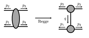
Figure 4: Illustration of the Regge-kinematic region (right), obtained from general kinematics (left) by taking the limit eq. 292. The grey blobs group final-state momenta where no strict rapidity ordering is assumed.

The MRK limit is the straightforward generalisation of this limit to the multi-parton case. In this paper we only consider the MRK limit of $2\to 3$ scattering,

$$y_{3}\gg y_{4}\gg y_{5}\,,\qquad\qquad|p_{3\perp}|\sim|p_{4\perp}|\sim|p_{5\perp}|\,.$$ (293)

The momenta flowing in the $t$-channels are $q_{1}=-p_{2}-p_{3}$ and $q_{2}=p_{5}+p_{1}$, that is, $t_{1}=q_{1}^{2}$ and $t_{2}=q_{2}^{2}$.

As stated in the introduction, the NMRK limit (also known as a quasi-multi-Regge kinematic or QMRK limit) is given by relaxing one of these strict rapidity orderings. The focus of this paper is on $2\to 3$ scattering, which has a rich structure of nested NMRK and MRK limits, illustrated in fig. 5. We restrict to the canonical ordering of particles, and, without loss of generality, only consider the forward NMRK limit, that is,

$$y_{3}\sim y_{4}\gg y_{5}\,,\qquad\qquad|p_{3\perp}|\sim|p_{4\perp}|\sim|p_{5\perp}|\,.$$ (294)

We note that two different MRK limits can be reached from eq. 294. In addition to the canonical MRK limit eq. 293, the limit

$$y_{4}\gg y_{3}\gg y_{5}\,,\qquad\qquad|p_{3\perp}|\sim|p_{4\perp}|\sim|p_{5\perp}|\,,$$ (295)

is also a boundary of the forward NMRK limit. We will refer to the region eq. 295 as the ${\mathrm{MRK}^{\prime}}$ limit, and likewise denote the relevant $t$-channel invariant by a prime, that is, $t_{1}^{\prime}=(q_{1}^{\prime})^{2}$ with $q_{1}^{\prime}=-p_{2}-p_{4}$. The relationship between the MRK, ${\mathrm{MRK}}^{\prime}$ and forward NMRK limits is depicted in fig. 6.

In practice, to obtain the (N)MRK limit of rational functions, we first implement the explicit representation of spinor products given in section A.1, and then map to the minimal set of variables described in section 3.

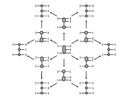
Figure 5: Illustration of the 3 forward NMRK, 3 backward NMRK and 3! MRK limits which can be obtained from a $2\to 3$ scattering process in general kinematics.

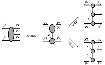
Figure 6: Illustration of the heirarchy of limits relevant for this paper. Starting from general kinematics (left) the forward NMRK region (centre) is reached by taking the limit eq. 294. The further MRK and ${\mathrm{MRK}}^{\prime}$ regions can be reached by taking the limits eq. 293 or eq. 295 respectively, which are the rapidity boundaries of the NMRK region.

Appendix B Special Functions

In this section we list the special functions used in this paper. The only divergent special function we us is the massless bubble integral,

$$K_{0}(x)=\frac{1}{\epsilon}+2-\log(-x)+\mathcal{O}(\epsilon)\,.$$ (296)

We use the following weight-1 functions, which are non-singular as $x\to 1$ Bern:1993mq

$$L_{0}(x) =\frac{\log(x)}{1-x}\,,$$ (297)

$$L_{1}(x) =\frac{\log(x)+1-x}{(1-x)^{2}}\,,$$ (298)

$$L_{2}(x) =\frac{1}{(1-x)^{3}}\left[\log(x)-\frac{x}{2}+\frac{1}{2x}\right]\,,$$ (299)

and we use the following weight-2 functions, which are non-singular as $x+y\to 1$

$$Ls_{-1}(x,y) ={\rm Li_{2}}(1-x)+{\rm Li_{2}}(1-y)+\log(x)\log(y)-\frac{\pi^{2}}{6}\,,$$ (300)

$$Ls_{1}(x,y) =\frac{1}{(1-x-y)^{2}}\bigg{[}Ls_{-1}(x,y)+(1-x-y)\left[L_{0}(x)+L_{0}(y)\right]\bigg{]}\,.$$ (301)

For $x>0$, the argument of the $L_{i}$ functions can be inverted using

$$L_{0}\left(\frac{1}{x}\right) =x\,L_{0}(x)\,,$$ (302)

$$L_{1}\left(\frac{1}{x}\right) =-x^{2}\,L_{1}(x)-x\,,$$ (303)

$$L_{2}\left(\frac{1}{x}\right) =x^{3}\,L_{2}(x)\,.$$ (304)

It is often necessary to write the $L_{i}$ functions in terms of functions with a higher or lower index so that the resulting coefficients are free from unphysical singularities. To this end we list explicitly the identities

$$L_{0}\left(x\right) =(1-x)\,L_{1}(x)-1=(1-x)^{2}\,L_{2}\left(x\right)-\left(\frac{1+x}{2x}\right)\,,$$ (305)

$$L_{1}\left(x\right) =(1-x)\,L_{2}(x)-\frac{1}{2x}\,.$$ (306)

We analytically continue these functions by giving all Mandelstam invariants a small positive imaginary part, $s\to s+i0$. For logarithms of ratios of invariants, this prescription yields

$$\log\left(\frac{-s_{1}}{-s_{2}}\right)=\log\left(\left|\frac{s_{1}}{s_{2}}\right|\right)-i\pi\left(\Theta(s_{1})-\Theta(s_{2})\right)$$ (307)

The analytic continuation of the dilogarithm is given in ref. vanHameren:2005ed .

References

- (1) L.N. Lipatov, Reggeization of the Vector Meson and the Vacuum Singularity in Nonabelian Gauge Theories, Sov. J. Nucl. Phys. 23 (1976) 338.
- (2) V. Del Duca, S. Druc, J.M. Drummond, C. Duhr, F. Dulat, R. Marzucca et al., All-order amplitudes at any multiplicity in the multi-Regge limit, Phys. Rev. Lett. 124 (2020) 161602 [1912.00188].
- (3) V. Del Duca, C. Duhr and V.A. Smirnov, An Analytic Result for the Two-Loop Hexagon Wilson Loop in = 4 SYM, JHEP 03 (2010) 099 [0911.5332].
- (4) V. Del Duca, C. Duhr and V.A. Smirnov, The Two-Loop Hexagon Wilson Loop in = 4 SYM, JHEP 05 (2010) 084 [1003.1702].
- (5) L.J. Dixon and M. von Hippel, Bootstrapping an NMHV amplitude through three loops, JHEP 10 (2014) 065 [1408.1505].
- (6) J.M. Henn and B. Mistlberger, Four-Gluon Scattering at Three Loops, Infrared Structure, and the Regge Limit, Phys. Rev. Lett. 117 (2016) 171601 [1608.00850].
- (7) S. Caron-Huot, L.J. Dixon, A. McLeod and M. von Hippel, Bootstrapping a Five-Loop Amplitude Using Steinmann Relations, Phys. Rev. Lett. 117 (2016) 241601 [1609.00669].
- (8) O. Almelid, C. Duhr, E. Gardi, A. McLeod and C.D. White, Bootstrapping the QCD soft anomalous dimension, JHEP 09 (2017) 073 [1706.10162].
- (9) S. Caron-Huot, L.J. Dixon, F. Dulat, M. von Hippel, A.J. McLeod and G. Papathanasiou, Six-Gluon amplitudes in planar = 4 super-Yang-Mills theory at six and seven loops, JHEP 08 (2019) 016 [1903.10890].
- (10) G. Falcioni, E. Gardi, N. Maher, C. Milloy and L. Vernazza, Scattering amplitudes in the Regge limit and the soft anomalous dimension through four loops, JHEP 03 (2022) 053 [2111.10664].
- (11) F. Caola, A. Chakraborty, G. Gambuti, A. von Manteuffel and L. Tancredi, Three-loop gluon scattering in QCD and the gluon Regge trajectory, 2112.11097.
- (12) A.R. White, Signature, factorization and unitarity in multi-regge theory - the five-point function, Nucl. Phys. B 67 (1973) 189.
- (13) R.C. Brower, C.E. DeTar and J.H. Weis, Regge Theory for Multiparticle Amplitudes, Phys. Rept. 14 (1974) 257.
- (14) J. Bartels, L.N. Lipatov and A. Sabio Vera, BFKL Pomeron, Reggeized gluons and Bern-Dixon-Smirnov amplitudes, Phys. Rev. D 80 (2009) 045002 [0802.2065].
- (15) E.P. Byrne, V. Del Duca, L.J. Dixon, E. Gardi and J.M. Smillie, One-loop central-emission vertex for two gluons in = 4 super Yang-Mills theory, JHEP 08 (2022) 271 [2204.12459].
- (16) E.A. Kuraev, L.N. Lipatov and V.S. Fadin, Multi - Reggeon Processes in the Yang-Mills Theory, Sov. Phys. JETP 44 (1976) 443.
- (17) P.D.B. Collins, An Introduction to Regge Theory and High-Energy Physics, Cambridge Monographs on Mathematical Physics, Cambridge Univ. Press, Cambridge, UK (5, 2009), 10.1017/CBO9780511897603.
- (18) C.D. White, Aspects of High Energy Scattering, SciPost Phys. Lect. Notes 13 (2020) 1 [1909.05177].
- (19) S. Mizera, Physics of the analytic S-matrix, Phys. Rept. 1047 (2024) 1 [2306.05395].
- (20) E.A. Kuraev, L.N. Lipatov and V.S. Fadin, The Pomeranchuk Singularity in Nonabelian Gauge Theories, Sov. Phys. JETP 45 (1977) 199.
- (21) I.I. Balitsky and L.N. Lipatov, The Pomeranchuk Singularity in Quantum Chromodynamics, Sov. J. Nucl. Phys. 28 (1978) 822.
- (22) V. Del Duca, An introduction to the perturbative QCD pomeron and to jet physics at large rapidities, hep-ph/9503226.
- (23) J.R. Forshaw and D.A. Ross, Quantum Chromodynamics and the Pomeron, vol. 9, Oxford University Press (1998), 10.1017/9781009290111.
- (24) V.S. Fadin, BFKL news, in LAFEX International School on High-Energy Physics (LISHEP 98) Session A: Particle Physics for High School Teachers - Session B: Advanced School in HEP - Session C: Workshop on Diffractive Physics, pp. 742–776, 7, 1998 [hep-ph/9807528].
- (25) V.S. Fadin, R. Fiore, M.G. Kozlov and A.V. Reznichenko, Proof of the multi-Regge form of QCD amplitudes with gluon exchanges in the NLA, Phys. Lett. B639 (2006) 74 [hep-ph/0602006].
- (26) V.S. Fadin, M.G. Kozlov and A.V. Reznichenko, Gluon Reggeization in Yang-Mills Theories, Phys. Rev. D92 (2015) 085044 [1507.00823].
- (27) V.S. Fadin and L.N. Lipatov, BFKL pomeron in the next-to-leading approximation, Phys. Lett. B429 (1998) 127 [hep-ph/9802290].
- (28) M. Ciafaloni and G. Camici, Energy scale(s) and next-to-leading BFKL equation, Phys. Lett. B430 (1998) 349 [hep-ph/9803389].
- (29) A.V. Kotikov and L.N. Lipatov, NLO corrections to the BFKL equation in QCD and in supersymmetric gauge theories, Nucl. Phys. B582 (2000) 19 [hep-ph/0004008].
- (30) A.V. Kotikov and L.N. Lipatov, DGLAP and BFKL equations in the =4 supersymmetric gauge theory, Nucl. Phys. B661 (2003) 19 [hep-ph/0208220].
- (31) V. Fadin, Chapter 4: BFKL — Past and Future, in From the Past to the Future, J. Bartels, V. Fadin, E. Levin, A. Levy, V. Kim and A. Sabio-Vera, eds., pp. 63–90 (2021), DOI [2012.11931].
- (32) S. Caron-Huot, E. Gardi and L. Vernazza, Two-parton scattering in the high-energy limit, JHEP 06 (2017) 016 [1701.05241].
- (33) V. Del Duca and E.W.N. Glover, The High-energy limit of QCD at two loops, JHEP 10 (2001) 035 [hep-ph/0109028].
- (34) V.S. Fadin and L.N. Lipatov, Reggeon cuts in QCD amplitudes with negative signature, Eur. Phys. J. C 78 (2018) 439 [1712.09805].
- (35) G. Falcioni, E. Gardi, N. Maher, C. Milloy and L. Vernazza, Disentangling the Regge Cut and Regge Pole in Perturbative QCD, Phys. Rev. Lett. 128 (2022) 132001 [2112.11098].
- (36) V.S. Fadin, Three-Reggeon Cuts in QCD Amplitudes, Phys. Atom. Nucl. 84 (2021) 100.
- (37) V. Del Duca, R. Marzucca and B. Verbeek, The gluon Regge trajectory at three loops from planar Yang-Mills theory, JHEP 01 (2022) 149 [2111.14265].
- (38) F. Caola, A. Chakraborty, G. Gambuti, A. von Manteuffel and L. Tancredi, Three-loop helicity amplitudes for quark-gluon scattering in QCD, JHEP 12 (2022) 082 [2207.03503].
- (39) V.S. Fadin, M. Fucilla and A. Papa, One-loop Lipatov vertex in QCD with higher -accuracy, JHEP 04 (2023) 137 [2302.09868].
- (40) B. Agarwal, F. Buccioni, F. Devoto, G. Gambuti, A. von Manteuffel and L. Tancredi, Five-Parton Scattering in QCD at Two Loops, 2311.09870.
- (41) G. De Laurentis, H. Ita, M. Klinkert and V. Sotnikov, Double-Virtual NNLO QCD Corrections for Five-Parton Scattering: The Gluon Channel, 2311.10086.
- (42) G. De Laurentis, H. Ita and V. Sotnikov, Double-Virtual NNLO QCD Corrections for Five-Parton Scattering: The Quark Channels, 2311.18752.
- (43) V. Del Duca, G. Falcioni, L. Magnea and L. Vernazza, Analyzing high-energy factorization beyond next-to-leading logarithmic accuracy, JHEP 02 (2015) 029 [1409.8330].
- (44) V.S. Fadin and L.N. Lipatov, Higher order corrections to QCD scattering amplitudes in a multi-Regge kinematics, Nucl. Phys. B Proc. Suppl. 29 (1992) 93.
- (45) V.S. Fadin and R. Fiore, Quark contribution to the gluon-gluon - reggeon vertex in QCD, Phys. Lett. B 294 (1992) 286.
- (46) V.S. Fadin, R. Fiore and A. Quartarolo, Reggeization of quark quark scattering amplitude in QCD, Phys. Rev. D 53 (1996) 2729 [hep-ph/9506432].
- (47) V. Del Duca and C.R. Schmidt, Virtual next-to-leading corrections to the impact factors in the high-energy limit, Phys. Rev. D 57 (1998) 4069 [hep-ph/9711309].
- (48) V. Del Duca, A. Frizzo and F. Maltoni, Factorization of tree QCD amplitudes in the high-energy limit and in the collinear limit, Nucl. Phys. B 568 (2000) 211 [hep-ph/9909464].
- (49) E.N. Antonov, L.N. Lipatov, E.A. Kuraev and I.O. Cherednikov, Feynman rules for effective Regge action, Nucl. Phys. B 721 (2005) 111 [hep-ph/0411185].
- (50) C. Duhr, New techniques in QCD, Ph.D. thesis, Louvain U., CP3, 2009.
- (51) M. Canay and V. Del Duca, One-loop impact factor for the emission of two gluons, JHEP 06 (2021) 034 [2103.16593].
- (52) Z. Bern, L.J. Dixon and D.A. Kosower, One loop corrections to five gluon amplitudes, Phys. Rev. Lett. 70 (1993) 2677 [hep-ph/9302280].
- (53) Z. Bern, L.J. Dixon and D.A. Kosower, One loop corrections to two quark three gluon amplitudes, Nucl. Phys. B 437 (1995) 259 [hep-ph/9409393].
- (54) M. Sjödahl, ColorMath - A package for color summed calculations in SU(Nc), Eur. Phys. J. C 73 (2013) 2310 [1211.2099].
- (55) V. Del Duca, Equivalence of the Parke-Taylor and the Fadin-Kuraev-Lipatov amplitudes in the high-energy limit, Phys. Rev. D 52 (1995) 1527 [hep-ph/9503340].
- (56) V. Del Duca, Next-to-leading corrections to the BFKL equation, Frascati Phys. Ser. 5 (1996) 463 [hep-ph/9605404].
- (57) V.S. Fadin and L.N. Lipatov, Radiative corrections to QCD scattering amplitudes in a multi - Regge kinematics, Nucl. Phys. B 406 (1993) 259.
- (58) S. Catani, M.H. Seymour and Z. Trocsanyi, Regularization scheme independence and unitarity in QCD cross-sections, Phys. Rev. D 55 (1997) 6819 [hep-ph/9610553].
- (59) V.S. Fadin, R. Fiore and A. Quartarolo, Radiative corrections to quark quark reggeon vertex in QCD, Phys. Rev. D 50 (1994) 2265 [hep-ph/9310252].
- (60) J. Bartels, High-Energy Behavior in a Nonabelian Gauge Theory (II): First Corrections to Beyond the Leading Approximation, Nucl. Phys. B 175 (1980) 365.
- (61) V.S. Fadin, R. Fiore and A. Quartarolo, Quark contribution to the reggeon - reggeon - gluon vertex in QCD, Phys. Rev. D 50 (1994) 5893 [hep-th/9405127].
- (62) V. Del Duca and C.R. Schmidt, Virtual next-to-leading corrections to the Lipatov vertex, Phys. Rev. D 59 (1999) 074004 [hep-ph/9810215].
- (63) M.D. Schwartz, K. Yan and H.X. Zhu, Factorization Violation and Scale Invariance, Phys. Rev. D 97 (2018) 096017 [1801.01138].
- (64) V. Del Duca, Real next-to-leading corrections to the multi - gluon amplitudes in the helicity formalism, Phys. Rev. D 54 (1996) 989 [hep-ph/9601211].
- (65) M.T. Grisaru, H.N. Pendleton and P. van Nieuwenhuizen, Supergravity and the S Matrix, Phys. Rev. D 15 (1977) 996.
- (66) V. Del Duca, L.J. Dixon and F. Maltoni, New color decompositions for gauge amplitudes at tree and loop level, Nucl. Phys. B 571 (2000) 51 [hep-ph/9910563].
- (67) Z. Bern, L.J. Dixon, D.C. Dunbar and D.A. Kosower, One loop n point gauge theory amplitudes, unitarity and collinear limits, Nucl. Phys. B425 (1994) 217 [hep-ph/9403226].
- (68) Z. Bern, L.J. Dixon, D.C. Dunbar and D.A. Kosower, Fusing gauge theory tree amplitudes into loop amplitudes, Nucl. Phys. B 435 (1995) 59 [hep-ph/9409265].
- (69) Z. Bern and D.A. Kosower, The Computation of loop amplitudes in gauge theories, Nucl. Phys. B 379 (1992) 451.
- (70) Z. Kunszt, A. Signer and Z. Trocsanyi, One loop helicity amplitudes for all 2 — 2 processes in QCD and N=1 supersymmetric Yang-Mills theory, Nucl. Phys. B 411 (1994) 397 [hep-ph/9305239].
- (71) M.B. Green, J.H. Schwarz and L. Brink, N=4 Yang-Mills and N=8 Supergravity as Limits of String Theories, Nucl. Phys. B 198 (1982) 474.
- (72) A. van Hameren, J. Vollinga and S. Weinzierl, Automated computation of one-loop integrals in massless theories, Eur. Phys. J. C 41 (2005) 361 [hep-ph/0502165].