Interactive Visualization of Time-Varying Flow Fields
Using Particle Tracing Neural Networks

Abstract

Lagrangian representations of flow fields have gained prominence for enabling fast, accurate analysis and exploration of time-varying flow behaviors. In this paper, we present a comprehensive evaluation to establish a robust and efficient framework for Lagrangian-based particle tracing using deep neural networks (DNNs). Han et al. (2021) first proposed a DNN-based approach to learn Lagrangian representations and demonstrated accurate particle tracing for an analytic 2D flow field. In this paper, we extend and build upon this prior work in significant ways. First, we evaluate the performance of DNN models to accurately trace particles in various settings, including 2D and 3D time-varying flow fields, flow fields from multiple applications, flow fields with varying complexity, as well as structured and unstructured input data. Second, we conduct an empirical study to inform best practices with respect to particle tracing model architectures, activation functions, and training data structures. Third, we conduct a comparative evaluation against prior techniques that employ flow maps as input for exploratory flow visualization. Specifically, we compare our extended model against its predecessor by Han et al. (2021), as well as the conventional approach that uses triangulation and Barycentric coordinate interpolation. Finally, we consider the integration and adaptation of our particle tracing model with different viewers. We provide an interactive web-based visualization interface by leveraging the efficiencies of our framework, and perform high-fidelity interactive visualization by integrating it with an OSPRay-based viewer. Overall, our experiments demonstrate that using a trained DNN model to predict new particle trajectories requires a low memory footprint and results in rapid inference. Following the best practices for large 3D datasets, our deep learning approach is shown to require approximately 46 times less memory while being more than 400 times faster than the conventional methods.

Our web-based visualization interface, integrated with our particle tracing neural networks, enables users to visualize and explore large 3D time-varying flow fields interactively. The interface offers 3D visualization of pathlines and user-uploaded scalar fields, along with a variety of configuration options for seed placement and rendering parameter adjustments. In this example, the model trained on the ScalarFlow dataset was used to display pathlines, with the FTLE of the dataset serving as the scalar field defining the background volume and pathlines’ color mapping. The training dataset was generated using 100,000 seeds placed in the injection area of $[44,64]\times[0,7]\times[38,58]$ over 90 time steps. Three deep learning models, each trained for 30 time steps, were utilized in this case. It took one second to load the models and 2.7 seconds to infer 300 pathlines displayed in the visualization using a dual-socket workstation equipped with an NVIDIA Titan RTX GPU. The trained model’s total storage size is 78.6 MB, further reducing the space consumption required for saving the original flow maps by 46 times.

Introduction

Time-varying flow visualization is useful for validating, exploring, and gaining insight from computational fluid dynamics simulations. It typically requires the computation and rendering of a large number of particle trajectories, such as pathlines and finite-time Lyapunov exponents (FTLEs), which can be computationally expensive and memory intensive. Furthermore, these computational challenges limit the interactivity of flow visualization. To address these challenges, conventional approaches decouple the particle advection and the rendering process to accelerate the visualization performance. For instance, pathlines are pre-computed and then visualized by a texture-based approach [31] or distributed to a high-performance computing system [3].

Deep learning techniques are promising in addressing these computational challenges in time-varying flow visualization. They provide compact representations, have reduce memory footprints, and provide fast inference capabilities. There have been recent advancements in applying deep learning to various aspects of fluid dynamics [8]. Concurrently, the scientific visualization community has increasingly utilized deep learning in the visualization pipeline [40, 59], and specifically in the analysis and visualization of time-varying flow fields [30, 48, 4, 29].

Recently, Han et al. [30] provided a first step toward utilizing a deep learning approach for time-varying particle tracing. They employed a multi-layer perceptron (MLP) model to reconstruct Lagrangian-based flow maps. Whereas their results highlighted the advantages of scientific deep learning such as reduced memory footprints and efficient inference, their method was limited to a 2D analytic flow and lacked empirical evidence to showcase the broader applicability of deep learning in time-varying flow visualization.

In this paper, we provide an in-depth study of MLP-based particle tracing deep learning models in capturing Lagrangian representations of time-varying flows and demonstrate their capability in enabling fast and accurate visualization of various flow regimes. The workflow of our deep learning approach is illustrated in Fig. 1. We advance beyond the particle tracing model of Han et al. [30] by conducting a comprehensive evaluation of the MLP-based models against the conventional approach. Our long term goal is to build a robust and efficient framework for Lagrangian-based flow visualization using deep learning. To that end, we empirically establish best practices in designing MLP-based models for flow reconstruction. Our contributions include:

• We evaluate how effectively MLP-based models reconstruct particle trajectories across a diverse collection of 2D and 3D flow fields, encompassing structured and unstructured data.

• We perform an in-depth analysis of particle tracing MLP models that includes: examining the effects of various activation functions, discerning the influence of model architectures, gauging the impact of flow complexity, and evaluating the effects of different training data structures.

• We performed a comparative analysis of our MLP models against prior particle tracing methods that utilize flow maps for exploratory flow visualization, including the MLP model of Han et al. [30] and conventional interpolation techniques.

• We assess the practical performance of deploying our trained models through both web-based Javascript and high-performance C++ libraries. This evaluation offers an in-depth understanding of how the neural network performs in real-world applications.

• We investigate model pruning techniques that enhance inference efficiency without compromising accuracy by judiciously discarding non-essential model weights.

• We introduce web-based and OSPRay-integrated viewers to assess the practical performance of our particle tracing models. Using Lagrangian-based flow representations, these tools provide interactive and seamless post hoc analysis and visualization of time-varying flow fields.

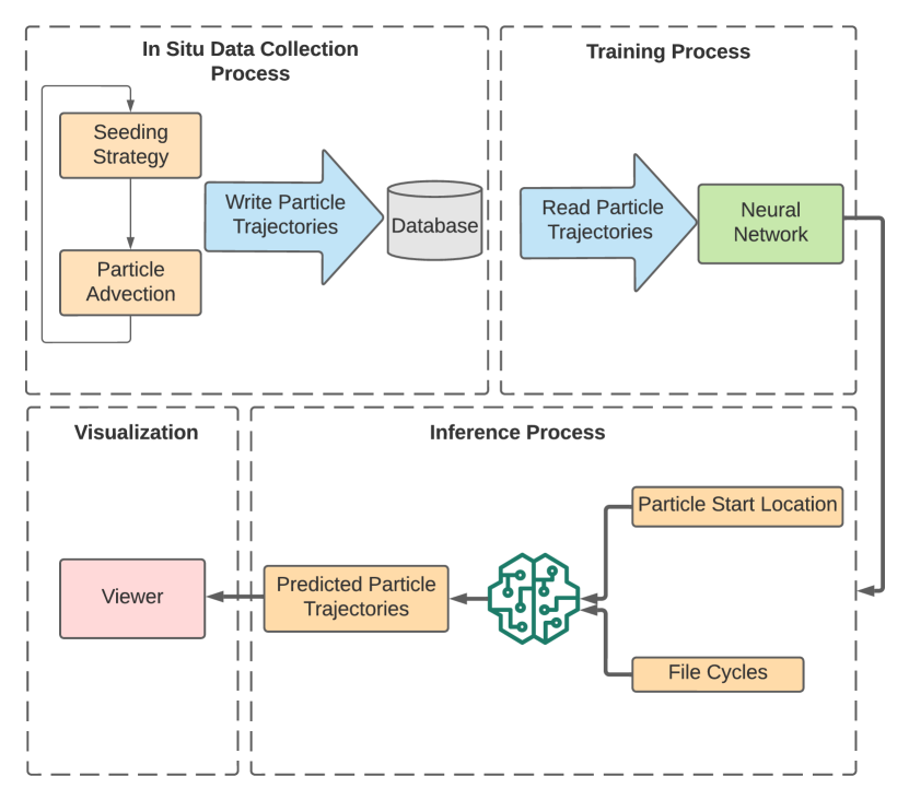
Figure 1: The workflow of our deep learning-based particle tracing model. The Lagrangian flow maps are created using in situ processing, saved to the database, and input into a neural network to learn the corresponding end locations based on particle start locations and file cycles. Once the model has been fully trained, new particle trajectories can be inferred from the model and visualized using the developed viewer.

1 Related Work

1.1 Lagrangian Flow Reconstruction and Visualization

Eulerian and Lagrangian reference frames are used to represent time-dependent vector fields. Eulerian-based representations store the velocity fields directly and calculate particle trajectories by integrating the velocity fields. Lagrangian representations encode the flow behaviors using flow maps $F^{t}_{t_{0}}$, which store the particle start location and end location from time $t_{0}$ to time $t$ and calculate arbitrary particle trajectories using interpolation. Even though the Eulerian method is fast to calculate, it requires dense temporal settings to reconstruct accurate results [11, 44, 1, 49, 46, 52]. In contrast, the Lagrangian-based method has received increased attention because it provides strong accuracy-storage proportions for exploration in temporally sparse settings [1, 45, 52, 51]. It also directly supports feature extraction [22, 53, 26, 21, 34].

In the Lagrangian representation of a time-varying vector field, information is encoded using flow maps, computed using in situ processing and analyzed post hoc. The reconstruction of new trajectories from the flow maps is a crucial aspect of post hoc analysis. Agranovsky et al. presented a multi-resolution interpolation scheme that begins with a base resolution and adds additional trajectories if the region contains interesting behaviors [2]. Bujack et al. [9] proposed representing particle trajectories by parameter curves, such as Bézier curves and Hermite splines, to improve the aesthetics of the derived trajectories. Chandler et al. [10] developed a k-d tree for efficient lookup of the particle neighborhoods during interpolation. However, to the best of our knowledge, none of the existing works investigate real-time exploration and visualization of Lagrangian-based flows. Two of the main challenges of interactive visualization during the post hoc analysis include reducing the I/O overhead of loading high-resolution flow maps, and accelerating the cell lookup of the particle neighborhoods. In addition, unstructured flow maps require time-consuming triangulation or tetrahedralization, making the interpolation process even slower.

In this paper, we empirically evaluate the use of deep learning for post hoc reconstruction and demonstrate the framework using an interactive web-based viewer for visualizing and analyzing the flow field. Using deep learning, flow maps can be represented by a model to conserve storage space. Importantly, interactive queries for arbitrary particle trajectories are possible without requiring intensive I/O operations for loading flow maps or computing the cell lookup procedure.

1.2 Deep Learning for Flow Visualization

Deep learning methods have become increasingly popular for flow visualization [40]. Examples of their widespread applications include the detection of eddies and vortices [38, 61, 56, 6, 14, 41, 12, 60, 20, 35, 7, 57], the segmentation of streamlines [39], the extraction of a stable reference frame from unsteady 2D vector fields [36], the optimization of data access patterns to boost computational performance in distributed memory particle advection [33], and the selection of a representative set of particle trajectories [50] using clustering methods grounded in deep learning [27, 37]. Furthermore, due to the scale of the flow data, data reduction and reconstruction is a widely discussed topic. Recent works have used low-resolution data [25, 23, 32] or 3D streamlines [28, 47] to reconstruct high-resolution vector fields. Using an efficient sub-pixel convolutional neural network (ESPCN) [54] and a super-resolution convolutional neural network (SRCNN) [13], Jakob et al. [34] upsampled 2D FTLE scalar fields produced from Lagrangian flow maps. Sahoo et al. [48] proposed a reconstruction technique for compressing time-varying vector fields by employing implicit neural networks. This approach involved learning through the integration scheme for vector fields.

Successfully visualizing flow map data relies on two critical factors: (1) accurate reconstruction of particle trajectories and (2) interactive visualization and exploration of these trajectories. Han et al. [30] employed a multi-layer perceptron (MLP) architecture to reconstruct Lagrangian-based flow maps for a 2D analytic dataset. Whereas they demonstrated the accuracy of reconstructing flow fields using a neural network, their study lacked quantitative and qualitative assessments across various datasets and an exploration of potential model architecture modifications. Furthermore, they did not investigate the benefits of rapid inference provided by deep learning models for interactive flow field visualization. Our research utilizes the exact Lagrangian representation of time-varying vector fields as data for neural networks, constructed using MLP and sinusoidal activation functions [55]. We assess our method through both qualitative and quantitative analyses on a variety of 2D and 3D datasets, including both structured and unstructured data. We conduct comprehensive experiments to investigate the impact of model architecture, flow complexity, and activation function. We also compare the performance of our deep-learning-based approach with the conventional post hoc interpolation method. Moreover, we utilize deep learning for interactive visualization and exploration during post hoc analysis of the Lagrangian-based flow field. We demonstrate that the neural network can be seamlessly integrated with various rendering APIs written in different programming languages and deployed on different platforms.

2 Lagrangian Analysis Using Deep Learning

Our neural network is designed to learn the behavior of a time-varying flow field. Before model training, we compute the Lagrangian flow maps by advecting massless particles in a time-varying flow field to generate the training datasets (Section 2.1). We adapt the MLP network architecture from Han et al. [30], which consists of an encoder and a decoder built with a series of fully connected (FC) layers. The starting location of a seed and a file cycle are individually input into encoders equipped with FC layers. The resulting encoded latent vectors are then concatenated and fed into the decoding layers, which predict the seed’s end location at the specified file cycle. Our neural network uses the same number of FC layers for the encoders of the seeds’ start location and file cycles to investigate the impact of the number of layers and the size of the latent vector on the performance. Moreover, we replace the ReLU activation function with the sinusoidal activation function, which Sitzmaan et al. [55] have validated to be suited for representing complex natural signals (Section 2.2).

2.1 Training Data Generation

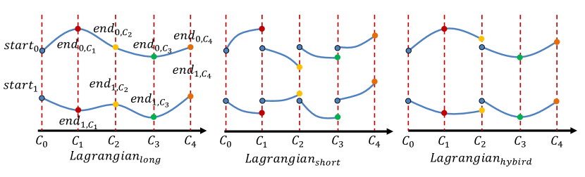
Figure 2: Illustration for $Lagrangian_{long}$, $Lagrangian_{short}$ and $Lagrangian_{hybird}$ methods using 1D particle trajectories. The x-axis represents the file cycle. Circles sharing the same color denote the same notation. The $Lagrangian_{long}$ extracts a single flow map with end locations at uniform time intervals along the trajectories. In contrast, the $Lagrangian_{short}$ extracts several short flow maps, resetting start seeds for each time interval. The $Lagrangian_{hybird}$ combines the strengths of both $Lagrangian_{long}$ and $Lagrangian_{short}$: it extracts the $Lagrangian_{short}$ flow maps, where each individual flow map follows the structure of a $Lagrangian_{long}$ flow map. $Lagrangian_{hybird}$ achieves both comprehensive domain coverage and comparable accuracy.

In this study, we replicate the training data generation of Han et al. [30], which uses two methods to extract flow maps — $Lagragian_{long}$ and $Lagrangian_{short}$ (Fig. 2). The $Lagrangian_{long}$ method extracts a single flow map composed of long particle trajectories with uniform temporal sampling for each integral curve. In contrast, the $Lagrangian_{short}$ method extracts multiple short flow maps, each comprising a set of seed locations and a set of end locations for each seed, where each end location corresponds to the displacement from the start location over non-overlapping intervals. Each method has its advantages and disadvantages. $Lagrangian_{short}$ flow maps provide good domain coverage since particles are periodically reset, but they may incur error propagation and accumulation when deriving new particle trajectories. $Lagrangian_{long}$ flow maps enable the derivation of new trajectories free of error propagation. However, as the integration time increases, the domain coverage of this method deteriorates and interpolation accuracy may reduce as particles diverge. To leverage the benefits of both methods, we introduce a hybrid method called $Lagrangian_{hybrid}$ (Fig. 2). This method extracts multiple $Lagrangian_{short}$ flow maps, where each map itself is a $Lagrangian_{long}$ flow map composed of particle trajectories with uniform temporal sampling for each integral curve instead of just storing the end locations. The training data structure is consistent across all three methods. However, there are slight differences in the inference processes for each method. We explore these differences and provide an accuracy comparison in Section 3.2.3.

For the seeding method, we place the initial seeds using a Sobol quasirandom sequence (Sobol), which has performed better than the pseudorandom number sequence and uniform grid [30]. The initial step in the production of training data is the placement of seeds in the spatial domain. After the placement of the seeds, particle trajectories are determined by shifting particles from $t$ to $t+\delta$, where $\delta$ represents one simulation time step. We refer to one simulation time step as a cycle. The cycle on which the end locations are saved is a file cycle, and the number of cycles between two successive file cycles is an interval.

Given a total temporal duration of $T$, seeds are inserted once at the beginning of time $t_{0}$ and traced until $T$ to produce flow maps using the $Lagrangian_{long}$ method. During the particle tracing process, intermediate locations are saved. Using the $Lagrangian_{short}$ method, particle tracing begins at time $t_{0}$ and concludes at time $t_{1}=t_{0}+\delta\times c$, where $c$ is the interval. The location at $t_{1}$ is then recorded, and the tracing seeds are reset until the next file cycle. This process is repeated until the last file cycle.

The $Lagrangian_{hybrid}$ method also begins particle tracing at time $t_{0}$ and terminates at $t_{1}=t_{0}+\delta\times c\times p$, where $C$ is the interval between the file cycle and $p$ is the number of intermediate locations to trace. The intermediate locations between $(t_{0},t_{1}]$ are recorded, and at time $t_{1}$, the seeds are reset. This process is continued until the final file cycle. The datasets used for training are saved in the NPY file format for efficient Python loading.

We built an $m\times n\times n$ array to store seed start locations and end locations across file cycles, where $m$ represents the number of seeds, $n$ represents the number of flow maps (file cycles). These training samples are arranged according to Eq. 1. Each training sample includes a start location $s_{i}$, the queried file cycle $c_{j}$, and the target end location at the queried file cycle $t_{i,j}$ (where $0\leq i\leq m-1$, $0\leq j\leq n-1$). We normalize the start location, the end location, and the queried file cycle to $[-1,1]$ before training. These bounds are used to scale the domain back to the original bounds during inference. The training dataset to our model is therefore

$$Input= \{\{s_{0},\,c_{0},\,t_{0,0}\},$$ (1)

$$\{s_{0},\,c_{1},\,t_{0,1}\},...,$$

$$\{s_{0},\,c_{n-1},\,t_{0,{n-1}}\},...,$$

$$\{s_{m-1},\,c_{n-1},\,t_{m-1,{n-1}}\}\}.$$

2.2 Network Architecture

Our neural network is based on the MLP architecture developed by Han et al. [30]. The encoder E takes the particle start locations coupled with file cycles as input and passes them through two sequences of FC layers that are then concatenated to form the latent vector input for the decoder D. The decoder D outputs the predicted end location, which is compared to the desired end location to calculate the loss. Although there is no universal model architecture suitable for all datasets, MLP offers flexibility in adjusting the size of the hidden vector and the number of layers to better suit different datasets. In Section 3.2.1, we examine how changing the number of layers and the dimension of the hidden vector affects the model performance. Additionally, Han et al. [30] observed that reconstruction errors increased as the number of file cycles a model learned increased. As flow maps store non-overlapping intervals, we train multiple models by partitioning the flow maps. However, using multiple models involves a trade-off between memory consumption and precision, which we investigate in Section 3.2.3.

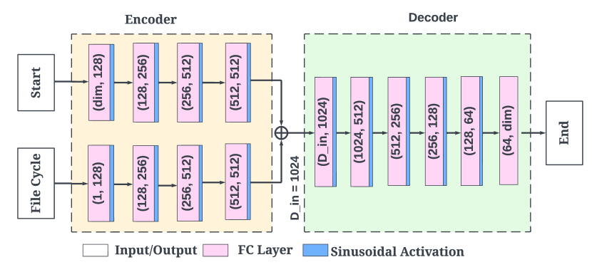
Figure 3: The MLP architecture of our neural network. The network takes the particle start location and the file cycles as input and outputs the particle end locations. The sinusoidal activation function is used after the fully connected layers in the model except the output layer.

The neural network is developed using Pytorch. We use the Adam optimizer with the hyperparameters $\beta_{1}=0.9$, $\beta_{2}=0.999$, and $\epsilon=1e-6$ along with a learning rate scheduler to reduce the current learning rate by a factor of 2 if the validation loss had not dropped for 5 epochs. We utilize an L1 loss as our loss function, which calculates the mean absolute error between the target and the predicted end locations:

$$loss(t_{i,j},\hat{t}_{i,j})=L1Loss(t_{i,j},\hat{t}_{i,j}),$$ (2)

where $t_{i,j}$ represents the target (ground truth) end location of seed $i$ at file cycle $c_{j}$ and $\hat{t}_{i,j}$ denotes the predicted end location ($0\leq i\leq m-1$ and $0\leq j\leq n-1$).

3 Results and Discussion

We first describe the datasets used in our evaluation (Section 3.1). To investigate the best practices involving deep-learning based particle tracing, we then evaluate the impact of model architecture, activation function, flow field complexity, and the training data structure on the performance of our model (Section 3.2). Additionally, we discuss model pruning to reduce the size of trainable parameters and evaluate the inference performance of our proposed neural network deployed by web-based JavaScript and high-performance C++ application (Section 3.3). We also conduct a comparative analysis against prior techniques that employ flow maps as input for exploratory flow visualization, such as the predecessor model of Han et al.[30] (Section 3.2.2) and the conventional Barycentric coordinate interpolation method (Section 3.4). Finally, we introduce a web-based viewer and an OSPRay-based viewer, offering two deployment options for the trained model and facilitating interactive flow visualization and exploration (Section 3.5). Our experiments employ a Dual RTX 3090s GPU for model training in a dual-socket workstation with two Intel Xeon E5-2640 v4 CPUs (40 logical cores at 2.4 GHz and 128 GB RAM) and an NVIDIA Titan RTX GPU for evaluation.

3.1 Datasets

In our studies, we utilize seven datasets, including four 3D datasets: ABC, Structured/Unstructured Half Cylinder ensembles, ScalarFlow, and Hurricane; and three 2D datasets: Double Gyre, Gerris Flow ensembles, and Structured/Unstructured Heated Cylinder.

Standard benchmark datasets such as the Double Gyre and ABC are commonly employed in fluid dynamics research, specifically for developing flow visualization techniques and tools. The Double Gyre flow field is defined within the spatial domain of $[0,2]\times[0,1]$, while the ABC flow field is defined within the spatial domain of $[0,2\pi]\times[0,2\pi]\times[0,2\pi]$. The equations used for the simulations are available in the supplemental material.

Heated Cylinder is a 2D unsteady simulation generated by a heated cylinder with Boussinesq Approximation [43, 24]. The simulation domain is $[-0.5,0.5]\times[-0.5,2.5]\times[0,20]$. Our experiments utilized the time span from 0 to 10. To demonstrate our approach, we employed both structured and unstructured datasets. The structured data possesses a grid resolution of $150\times 450$.

Gerris Flow is a 2D ensemble simulation done by Gerris flow solver [43, 34]. It contains 8000 datasets with the value of Reynolds number (Re) varying from a steady regime ($Re<50$) to periodic vortex shedding ($Re<200$) to turbulent flows ($Re>2000$) [34]. We have chosen datasets with Re value of 23.2, 101.6, 445.7, and 2352.5 to showcase the performance of our method for varying degrees of flow complexity. The grid resolution is $[X\times Y\times T]$ is $[512\times 512\times 1001]$ with the simulation domain as $[0,1]\times[0,1]\times[0,10]$.

Half Cylinder is a 3D ensemble of numerical simulations of an incompressible 3D flow around a half cylinder [43, 5]. We experimented with both structured and unstructured grids, selecting Re values of 160 and 320 to investigate the effects of varying turbulence degrees. The domain of the simulation is identified as $[-0.5,7.5]\times[-0.5,1.5]\times[-0.5,0.5]$. Both structured and unstructured datasets span 80 time steps. The structured dataset is designed with a grid resolution of $640\times 240\times 80$.

ScalarFlow is a large-scale, 3D reconstructions of real-world smoke plumes [15]. The spatial dimension is $[100\times 178\times 100]$, and the number of time steps is 150.

Hurricane is a simulation from the National Center for Atmospheric Research. The data dimension is $[500\times 500\times 100]$ with 47 time steps. We used the first 40 time steps and the region $[150,399]\times[150,399]\times[0,99]$ that contains the interesting features – the hurricane eye in our studies.

In our experiments, we considered a $\delta=0.01$ step size and $interval=5$ for the Double Gyre, ABC, Unstructured Heated Cylinder, and Gerris Flow datasets, a $\delta=0.1$ and $interval=1$ for the Half Cylinder, ScalarFlow and Hurricane datasets.

3.2 Model Evaluation

To evaluate the performance of the neural network, we first investigate the effect of model architecture parameters on performance, such as the number of layers and the size of the hidden vector (Section 3.2.1). Next, we compare our model using the sinusoidal activation function with previous work [30] that uses the ReLU activation function to demonstrate the advantages of the sinusoidal activation function (Section 3.2.2). Finally, we illustrate the performance of the neural network on the flow complexity using ensemble datasets and enhance the accuracy by training multiple models along the pathlines and examining the effectiveness of our $Lagrangian_{hybird}$ method (Section 3.2.3).

During the training phase, we generated an additional 10% of training data samples for validation. In the following testing results, each error instance represents the average distance between the predicted and target (ground truth) locations along a trajectory, as defined in Eq. 3.

$$error_{i}=\frac{1}{n}\sum_{j=0}^{n-1}loss(t_{i,j},\hat{t}_{i,j})$$ (3)

where $i$ represents the index of the new seed and $n$ is the number of end locations (file cycles) along the trajectories. $t_{i,j}$ is the target (ground truth) end location, and the $\hat{t}_{i,j}$ is the predicted end location. We placed 5,000 random seeds in the domain for all testing results presented below.

3.2.1 Impact of Model Architecture

In our experiments, we evaluated the qualitative and quantitative effects of varying the number of layers in the encoder and decoder as well as the dimension of the encoded latent vector. To evaluate our model, we used several datasets, including the Double Gyre, Gerris Flow with Reynolds numbers $Re=101.6$ and $Re=445.7$, ABC flow, and the unstructured Half Cylinder with Reynolds numbers $Re=160$ and $Re=320$. For benchmarking our model’s performance, we utilized 100 flow maps for each 2D dataset and 50 flow maps for each 3D dataset. For all datasets, we distributed seeds with the number of half of the grid resolution. However, in the case of the Half Cylinder datasets, to optimize training time, we strategically placed seeds only within the region defined by $[-0.5,0.5]\times[-0.5,0.5]\times[-0.5,0.5]$. This region encompasses the obstruction and areas of interest, allowing for more focused training.

In the experiments, we opted for encoder layer and decoder layer count of four, six, and eight. The encoded latent vector has dimensions of 1024 and 2048. Tab. 1 in the supplemental material displays the maximum, minimum, mean, and median errors associated with various combinations of encoder layers, decoder layers, and latent vector dimensions.

	Model(MB)		Training (hrs)		Inference (s)
[#E, #D]	1024	2048	1024	2048	1024	2048
[4, 4]	8.5	33.9	0.348	0.478	0.297	0.343
[4, 6]	8.6	34.5	0.368	0.488	0.277	0.397
[4, 8]	8.7	34.6	0.380	0.499	0.308	0.351
[6, 4]	8.6	34.3	0.379	0.491	0.282	0.375
[6, 6]	8.7	34.9	0.396	0.502	0.285	0.360
[6, 8]	8.8	35.0	0.410	0.511	0.279	0.354
[8, 4]	8.6	34.3	0.409	0.502	0.329	0.359
[8, 6]	8.8	35.0	0.425	0.512	0.283	0.376
[8, 8]	8.8	35.0	0.438	0.521	0.289	0.366

Table 1: The training and inference time results for models of varying sizes. Each row ($[E,D]$) represents the number of encoding layers ($E$) and decoding layers ($D$), and the hidden vector dimension is either 1024 or 2048. Training time was measured on 100K training samples with 20 flow maps, trained for 100 epochs, utilizing distributed data parallel. Inference time was evaluated on 5,000 seeds with 20 flow maps, using Pytorch in Python with CUDA.

Our model design achieved an acceptable error rate for all datasets. Our experiments revealed that the optimal model architecture depends on the specific dataset. For steady flow regimes, such as those observed in the Double Gyre and Gerris (Re 23.2), a smaller latent vector dimension resulted in higher accuracy. Conversely, for datasets exhibiting periodic vortex shedding, like Gerris (Re 101.6), and in 3D datasets, a larger latent vector dimension proved to be more effective than a smaller one. Furthermore, we observed a trend regarding the depth of encoding and decoding layers. In most cases, models with deeper layers, particularly those with 8 encoding or decoding layers, yielded less accurate inferences, performing the least effectively in our tests (Tab. 1 in supplemental material). When evaluating a neural network, model size is an important consideration, in addition to its inference accuracy. As shown in Table 1, model size increases with an increasing number of layers in both the encoder and decoder, and doubles when increasing the hidden vector size from 1024 to 2048. Moreover, a neural network with more parameters requires more time for both training and inference.

3.2.2 Impact of Activation Function

We compared our approach to the ReLU-based MLP model proposed by Han et al.[30] with the same model architecture, which includes five encoding layers for the seeds’ start location, seven encoding layers for the file cycles, a latent vector of dimension 1024, and six decoding layers. As recommended by Sitzmann et al. [55], we removed the LayerNorm and replaced the ReLU activation function in the original architecture with the sinusoidal function for our comparative study. For our experiments, we used the same datasets as described in Section 3.2.1. We set the learning rate to be $1e^{-4}$ for the ReLU-based MLP, as demonstrated to be the optimal choice in [30] and confirmed by our experiments. For our approach using the sinusoidal function, we used an optimal learning rate of $5e^{-4}$.

Fig. 4 shows the inference error of our sinusoidal-based MLP and the ReLU-based MLP. Our results indicate that the sinusoidal activation function significantly outperformed the ReLU activation function on all datasets tested. Furthermore, our method achieved these results using the same storage space as the model in [30] (which had a size of 8.4 MB), while greatly improving the accuracy.

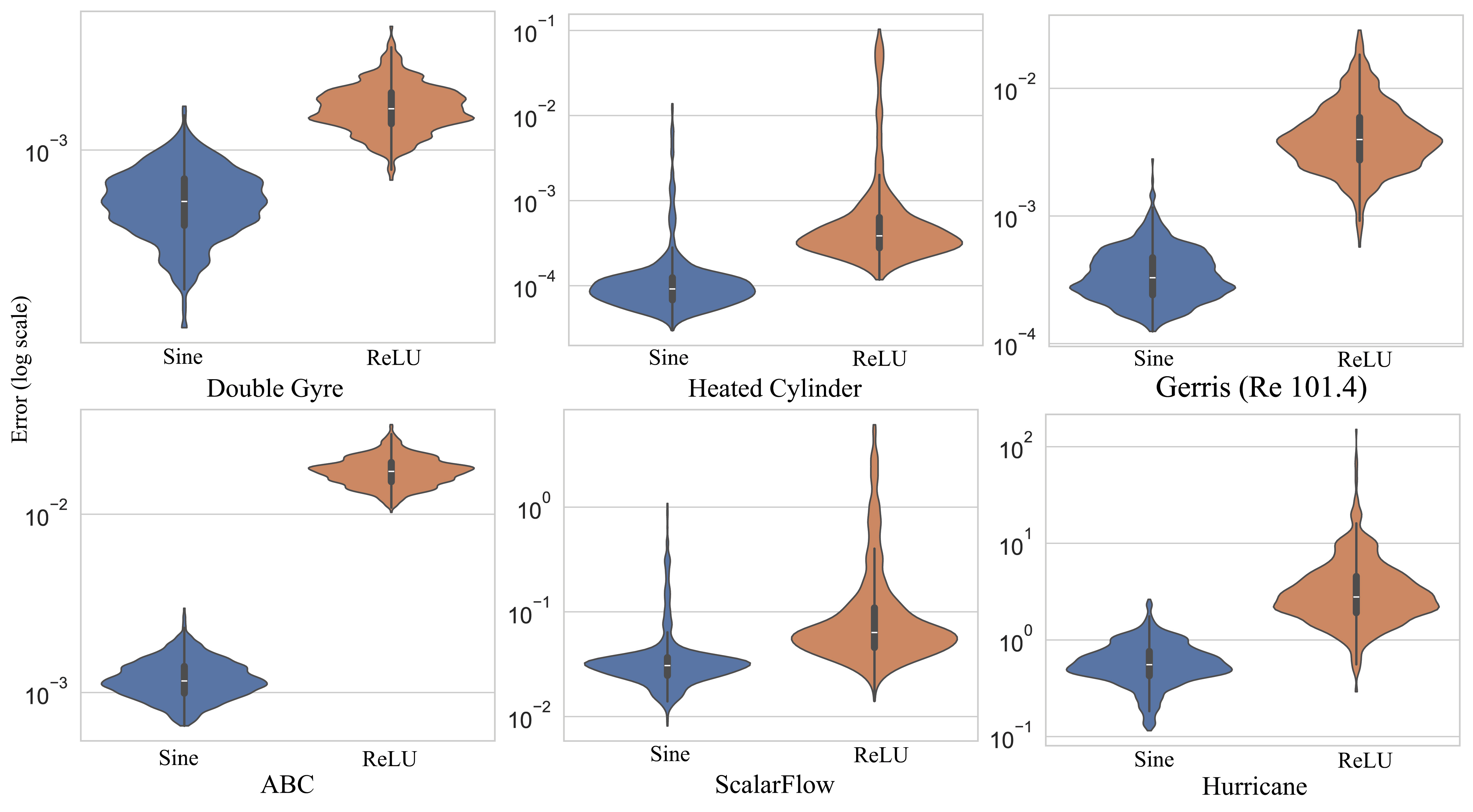
Figure 4: The error plot compares our sinusodial-based MLP with the ReLU-based MLP of Han et al. [30]. The sinusoidal activation function improves the inference accuracy significantly.

3.2.3 Impact of Flow Complexity

The optimal model architecture varies among datasets. Based on these findings, we investigated how the complexity of the flow affects the performance of our proposed deep learning model. We conducted an analysis on four different Gerris Flow datasets with varying Reynolds (Re) values: 23.2, 101.6, 445.7, and 2352.5, covering a range of flow regimes from steady ($Re<50$), periodic vortex shedding ($50<Re<200$), to turbulent flows ($Re>2000$) [34]. Each training dataset consisted of 500 time steps with an interval of 5, resulting in 100 flow maps for each dataset. To train our model, we used 262,144 seeds for each dataset and designed the model with four encoding layers, six decoding layers, and a 2048D latent vector.

Our results revealed that one of the limitations of our suggested method is the decline in inference accuracy as the underlying flow behavior becomes more complex. Specifically, we observed that the turbulence flow feature (Gerris with $Re=2352.5$) was the most challenging to learn (Fig. 5). Improving the ability to infer turbulent flow could be a focus of future research.

Prior work by Han et al. [30] showed that the $Lagrangian_{long}$ method results in fewer errors compared to the $Lagrangian_{short}$ method, despite a reduction in domain coverage over time. Consequently, our experiments focused solely on comparing the $Lagrangian_{long}$ and $Lagrangian_{hybrid}$ methods (Fig. 2). As shown in Fig. 5, the $Lagrangian_{hybrid}$ method consistently reduces median errors across all datasets when compared to the $Lagrangian_{long}$ method. In addition, our study explored the effect of diminishing the number of flow maps used per model on training accuracy. This was achieved by training two separate models, each with 50 flow maps, as opposed to a single model trained with 100 flow maps.

The findings, as depicted in Fig. 5, indicate that reducing the number of flow maps per model does not improve training accuracy when employing the $Lagrangian_{long}$ method. However, a slight decrease in errors was observed when implementing the $Lagrangian_{hybrid}$ method. Throughout the training phase, it was observed that the second model employing the $Lagrangian_{long}$ method exhibited errors approximately five times greater than those of the first model. We hypothesize that this increased error may be due to the greater difficulty in achieving model convergence, possibly attributed to the larger spatial gap between the initial seed locations and their corresponding end points in the second model.

Our findings suggest that $Lagrangian_{hybrid}$ has a higher accuracy than $Lagrangian_{long}$, and can also mitigate the error propagation issue of $Lagrangian_{short}$.

Figure 5: Violin plot depicting the inference errors for models trained on Gerris Flow datasets with varying Reynolds numbers, using either the $Lagrangian_{long}$ method with one or two models or the $Lagrangian_{hybrid}$ method with one or two models. These evaluations, conducted with 5,000 testing seeds, calculate errors as defined by Eq. 3. A comparison of violin plots of the same color across different datasets reveals that errors tend to increase as the flow behavior becomes more turbulent. Interestingly, using fewer flow maps for training in the $Lagrangian_{long}$ approach did not improve accuracy. Conversely, in the $Lagrangian_{hybrid}$ approach, using fewer flow maps actually led to a slightly decrease in median errors. Furthermore, the $Lagrangian_{hybrid}$ method effectively reduces error propagation while maintaining domain coverage.

3.3 Model Pruning and Inference Performance

3.3.1 Model Pruning

An MLP model can often contain more weights than necessary for a given task. The lottery ticket hypothesis suggests that a smaller subset of the network is responsible for the majority of the task [19]. This implies that a smaller model within the larger one can achieve the same level of accuracy. In order to create more efficient neural networks, we utilize model pruning techniques, specifically the novel algorithm proposed by Fang et al. [18] using DepGraph. This approach uses a magnitude pruning technique [16] that automatically identifies the most important connections in the neural network, resulting in a smaller, more efficient model. We perform the pruning interactively, removing some weights and then fine-tuning the model for an epoch before repeating the process until a certain percentage of the model is pruned. Note that we do not prune important layers, such as the last layer of the model, to ensure that the model’s output remains the same format. Utilizing structured pruning techniques allows us to create smaller, more efficient models that maintain the same level of accuracy as their larger counterparts.

A prime example of this is demonstrated in our experiments with the Hurricane dataset, where we were able to reduce the size of a model from 34.5 MB to just 13.7 MB while maintaining the same level of accuracy. This reduction in model size can lead to faster inference times, decreased memory requirements, and improved overall efficiency in neural network applications.

3.3.2 Inference Performance

In Section 3.2.1, we evaluated the inference speed of our models with different sizes using Pytorch in Python. In this section, we evaluated the inference performance of our neural network in the web-based viewer and OSPRay integration using the ABC and Hurricane datasets. For the ABC dataset, we built a model with a 1024D hidden vector, three encoding layers, and six decoding layers, resulting in a model size of 8.4 MB. For the Hurricane dataset, we constructed a model with a 2048D hidden vector, five encoding layers, and eight decoding layers. The original model had a size of 34.5 MB, but after pruning, the size reduced to 13.7 MB. The ABC dataset contains 20 flow maps, while the Hurricane dataset contains 30 flow maps.

We evaluated the performance of our viewers on two workstations - one with an Intel Xeon CPU and an NVIDIA Titan RTX GPU, and the other with an Intel NUC i7-8809G CPU (8 logical cores and 32 GB RAM). We measured the speed of rendering by scattering 100, 200, 300, 400, 500, and 1000 seeds across the domain for each dataset.

ABC - $Lagrangian_{long}$ - 8.4 MB
	Model Loading (s)	#100 (s)	#200 (s)	#300 (s)	#400 (s)	#500 (s)	#1000 (s)
ONNX + GPU	2.12	0.45	0.52	0.58	0.64	0.65	1.07
ONNX + CPU	1.69	0.39	0.82	1.06	1.41	1.84	3.19
Hurricane - $Lagrangian_{long}$ - 13.7 MB
ONNX + GPU	2.48	0.57	0.76	0.92	0.97	1.21	1.85
ONNX + CPU	1.81	0.72	1.45	2.48	2.99	3.32	6.07

(a) Performance evaluation of the web-based viewer deployed by ONNX Runtime web in JavaScript.

ABC - $Lagrangian_{long}$ - 8.4 MB
	Model Loading (s)	#100 (s)	#200 (s)	#300 (s)	#400 (s)	#500 (s)	#1000 (s)
ONNX + GPU	1.15	0.003	0.005	0.007	0.009	0.014	0.032
ONNX + CPU	0.072	0.11	0.22	0.33	0.41	0.54	0.95
Hurricane - $Lagrangian_{long}$ - 13.7 MB
ONNX + GPU	1.18	0.004	0.007	0.009	0.012	0.018	0.037
ONNX + CPU	0.11	0.16	0.26	0.41	0.54	0.68	1.29

(b) Performance evaluation of the OSPRay integration deployed by ONNX Runtime in C++.

Table 2: The inference performance of our web-based viewer (Table 2(a)) and OSPRay integration (Table 2(b)) with increasing numbers of seeds (#N where N represents the seed count) for the ABC and Hurricane datasets. We deployed the trained model using ONNX Runtime API. Performance is measured in seconds and experiments were conducted on a workstation using a CPU (20 threads) or a GPU (CUDA). Our viewers enable interactive inference and visualization of new trajectories with the $Lagrangian_{long}$ method using the GPU. The C++ API is at least five times faster than the JavaScript API. Furthermore, while the GPU outperforms the CPU in inference, it is slower in loading the model.

ABC - $Lagrangian_{long}$ - 8.4 MB
	Model Loading	#100	#200	#300	#400	#500	#1000
ONNX + CPU (s)	0.83	0.42	0.97	1.11	1.46	1.82	3.63
Hurricane - $Lagrangian_{long}$ - 13.7 MB
ONNX + CPU (s)	0.84	0.98	1.74	2.51	3.31	4.10	7.72

Table 3: Performance evaluation of our web-based viewer with increasing numbers of seeds for the ABC and Hurricane datasets. The experiments were conducted on an Intel NUC using a CPU with all eight threads. The ONNX Runtime API was used to deploy the trained model. The performance of using this low-end desktop has similar performance compared to the workstation, indicating the parallelism scheme of ONNX is not optimal. Further accelerations are required for interactive inference for the web-based viewer in future work.

Table 2 presents the model loading and inference speeds of our web viewer and OSPRay integration using a CPU with 20 threads and a GPU with CUDA on the workstation. With CUDA, our developed viewers can enable full interactivity for up to 1,000 new seeds in the inference pathlines. The motivation of deploying the trained neural network on a web browser is to enable users to access post hoc exploration more easily, without requiring a high-performance computer. As shown in Table 3, we observed similar performance results to those using the workstation (Table 2(a)), indicating that the parallel algorithm used by ORT is not optimal. Therefore, further improvement and acceleration of web-based deployment is required. Although the web-based viewer with a CPU is not fully interactive, it is still much faster than the conventional interpolation approach (Section 3.4).

3.4 Comparison with Interpolation Methods

To compute the trajectories of new start seeds, post hoc interpolation methods are applied after saving the basis Lagrangian flow maps through particle tracing. Conventional interpolation methods, including Barycentric coordinate and Shepard’s method, require the identification of the vicinity of the new seeds in the basis trajectories for computing a new particle trajectory. The methods for determining the neighborhoods rely on the structure of the basis flow maps. Delaunay triangulation can locate a cell in either a structured or unstructured data source containing a Lagrangian representation.

In our experiments, we compared the performance of our proposed approach to that of the conventional post hoc interpolation method, which includes loading the basis flow maps, creating the triangulation structure, and performing Barycentric coordinate interpolation.

			BC		DL
Datasets	#FM	Resolution	Computation (hrs)	Storage (MB)	Training (hrs)	Storage (MB)
Gerris (Re 23.2) [S]	100	$512\times 512$	0.072	683.8	0.93	8.6
Hurricane [S]	30	$150\times 150\times 100$	6.	1640.9	11.25	35.0
Heated Cylinder [U]	100	49,610	0.03	101.3	0.25	35.0
Heated Cylinder [S]	100	$150\times 450$	0.03	137.4	3.45	35.0
Half Cylinder (Re 160) [U]	50	102,752	0.71	139.2	0.50	34.5
Half Cylinder (Re 160) [S]	50	$80\times 80\times 80$	0.57	720.0	2.50	34.5

Table 4: Comparing the computation time and storage requirements of the deep-learning-based approach (DL) vs. the conventional post hoc interpolation (BC) using Delaunay triangulation and Barycentric coordinate interpolation. This table evaluates the time to compute basis flow maps and the duration of neural network training across various structured (S) and unstructured (U) datasets. It includes the number of flow maps ($\#FM$) and the resolution for each dataset. Additionally, it details the storage space needed for the basis flow map and the neural network. While our approach requires more time for neural network training, it consistently outperforms the conventional method in speed across all experiments (refer to Fig. 6) and reduces storage space requirements by three to 46 times compared to the conventional approach.

In our implementation, we utilized the CGAL [17] library to generate the triangulation structure and employed Threading Building Blocks [42] (TBB) to parallelize all processes, including (1) loading the basis flow maps, (2) triangulation, and (3) interpolation. Our deep learning strategy consists of three steps: (1) loading the learned model, (2) generating the input using seed start locations and file cycles, and (3) inferring results using the training model. In our studies, we implemented both methods in C++ and utilized ORT  with CUDA for the inference procedure of deep learning. For evaluations, we used two structured datasets (Gerris with Re 23.2 and Hurricane) and other two datasets (Heated Cylinder and Half Cylinder with Re 160) in both structured and unstructured formats. We computed the basis flow maps for structured datasets by placing seeds at each grid vertex to compute basis flow maps and utilizing Sobol seeds to generate training data. In the case of unstructured data, we used sparse seeds at the center of each cell.

Figure 6: Computation time comparison of deep-learning-based approach (DL) vs. conventional Barycentric coordinate interpolation approach (BC). This figure illustrates the time required for various tasks in both methods: loading basis flow maps, triangulation, and interpolation for the conventional approach, and training, model loading, and inference for the deep learning approach, across different structured and unstructured datasets. Both approaches utilized an equal number of seeds. Our results indicate that the DL approach was consistently faster than the BC approach in all experiments. Notably, it was about 426 times quicker for the hurricane dataset and at least three times faster for unstructured datasets. This significant speed advantage enables interactive flow visualization and exploration in large 3D datasets.

Figure 7: Violin plot showing a comparison of errors between our deep-learning-based method (DL) and the conventional Barycentric coordinate interpolation (BC) approach. ’S’ denotes structured data, while ’U’ signifies unstructured data. Overall, our approach achieves a threefold reduction in median error for structured datasets. Nevertheless, it is observed that our method tends to yield higher errors for unstructured datasets, particularly those trained with sparse seeding.

In Fig. 6 and Table 4, we compare the execution times and storage requirements of our proposed method with those of the conventional methods. Our approach is significantly faster than loading the basis flow maps for all structured datasets, taking less than two seconds to load the model. As shown in Fig. 6, our deep-learning strategy is approximately 426 times faster on the hurricane dataset and at least three times faster on the smallest unstructured heated cylinder dataset. Even without comparing the triangulation process, using a trained model saves significant time for interpolation.

Furthermore, our approach also requires less storage space. For instance, for the hurricane dataset, saving the trained model reduces storage space by a factor of 46. For the smallest unstructured heated cylinder dataset, our method reduces storage requirements by three times. Additionally, we can save even more space using our model pruning strategy (Section 3.3) in our deep learning-based approach.

While our approach has shown promising results, one limitation to consider is the extensive training time required. For instance, the hurricane dataset of 2.25 million seeds and 30 flow maps took approximately 11 hours to complete 100 epochs. However, it is important to note that this is a common issue associated with deep learning and can be potentially mitigated by utilizing more powerful hardware or developing new training procedures in the future.

As depicted in Fig. 7, we evaluated the inference accuracy of our approach in comparison to the conventional approach using Barycentric coordinate. On average, our proposed strategy reduces the inaccuracy by a factor of three for all structured datasets.

Fig. 8(b) showcases a comparison between the trajectories and FTLE as computed by our method and the established ground truth. This illustration highlights the effectiveness of our approach in predicting results more accurately than the conventional interpolation method, achieving this with a notable absence of visible visual artifacts.

However, it is worth noting that our current model exhibits a larger error rate when dealing with unstructured data, particularly for the 3D dataset such as the half cylinder, which employs sparse seeds for training. To overcome this limitation, we intend to explore an adaptive sampling strategy in our future work, which could aid in selecting important seeds for generating training data.

In summary, our proposed deep-learning-based method has the potential to substantially improve the accuracy on structured datasets, while also minimizing their storage requirements and expediting the interpolation procedure, when compared to the conventional post hoc interpolation approach.

(a) Gerris (Re 101.6).

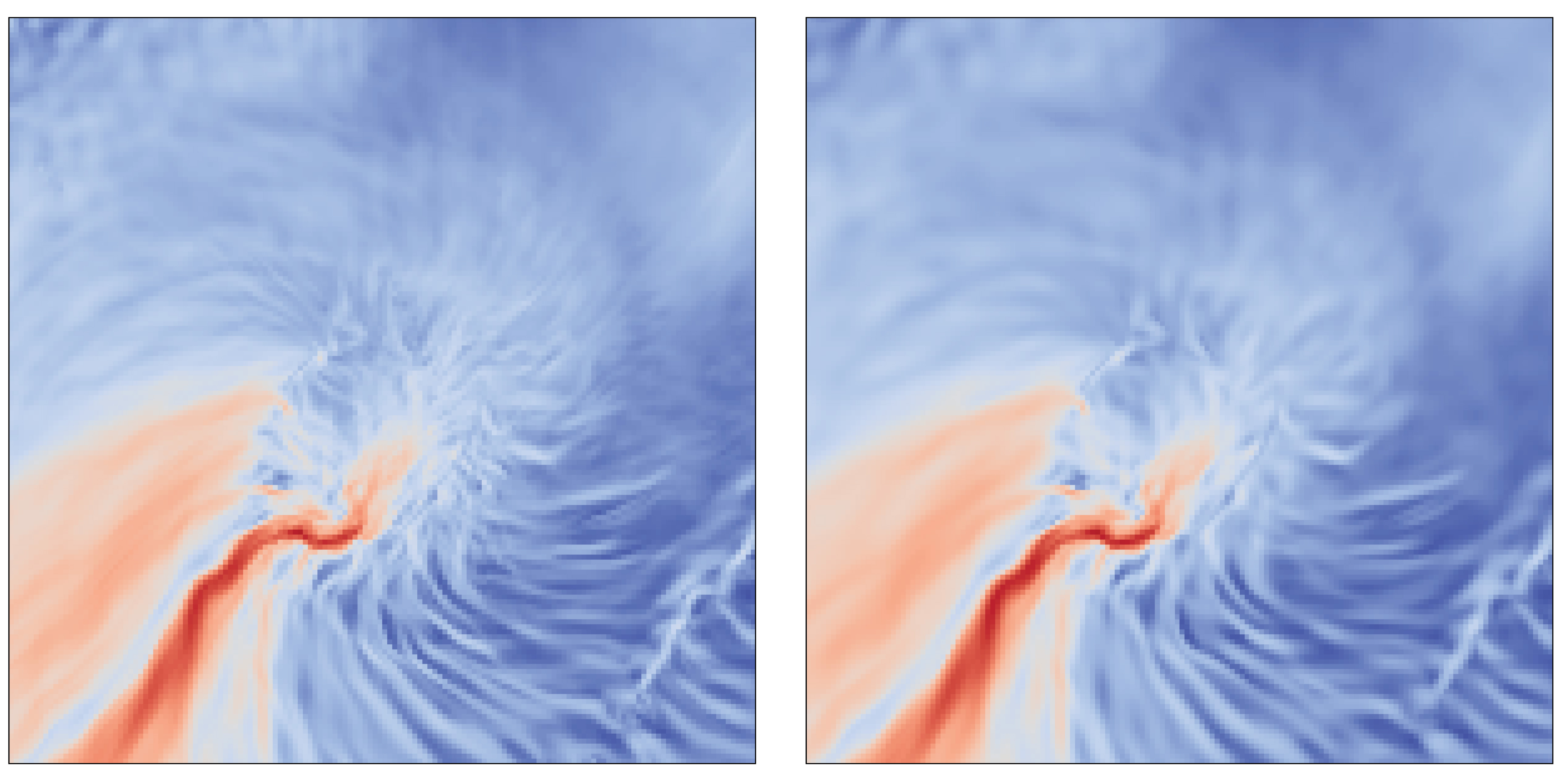
(b) Hurricane.

Fig. 8(a) provides a visual comparison against the ground truth trajectories (marked in red). The left side of the figure shows results from the Barycentric coordinate interpolation (BC), whereas the right side presents outcomes from our deep-learning approach (DL), with the computed trajectories highlighted in blue. Furthermore, Fig. 8(b) compares the ground truth FTLE on the left with the results computed using our method on the right. Our approach not only accurately traces pathlines but also yields FTLE visualizations that are in close alignment with the ground truth and are devoid of visual artifacts.

3.5 Interactive Visualization Tool for Post Hoc Analysis

Benefiting from our model’s minimal memory footprint and fast inference, we build a deep learning approach to accelerate the post hoc interpolation and visualization of Lagrangian flow maps, which is typically expensive due to I/O constraints and interpolation performance (Section 3.4). To facilitate the exploration of flow maps without requiring a powerful computer, we developed a web-based viewer that utilizes our neural network as the backend to accelerate the interpolation and visualization process. The viewer is implemented in JavaScript and is compatible with multiple platforms and popular web browsers, such as Safari, Chrome, and Firefox. The user interface of the web-based viewer includes control panels for model loading, seed placement, seed box configuration, scalars configuration, transfer function editing, and tracing. It also provides a primary viewer for presenting the visualization of pathlines, surfaces, and volumes, allowing users to engage with seed placement and visualization outcomes (Fig. 10). Details of the web viewer are described in supplemental material. We highlight a couple of visualization results in Fig. 9 and Fig. 10 respectively.

In addition to the web-based viewer, we have also integrated our neural network with the OSPRay [58] rendering engine to enable C++ implementation (see supplemental material). Our integration with the web-based viewer and OSPRay rendering engine is independent of the model architecture, allowing users to integrate their models easily by simply replacing the trace function. We highlight the visualization result of ScalarFlow in Fig. 11.

All of our source code is available on GitHub.

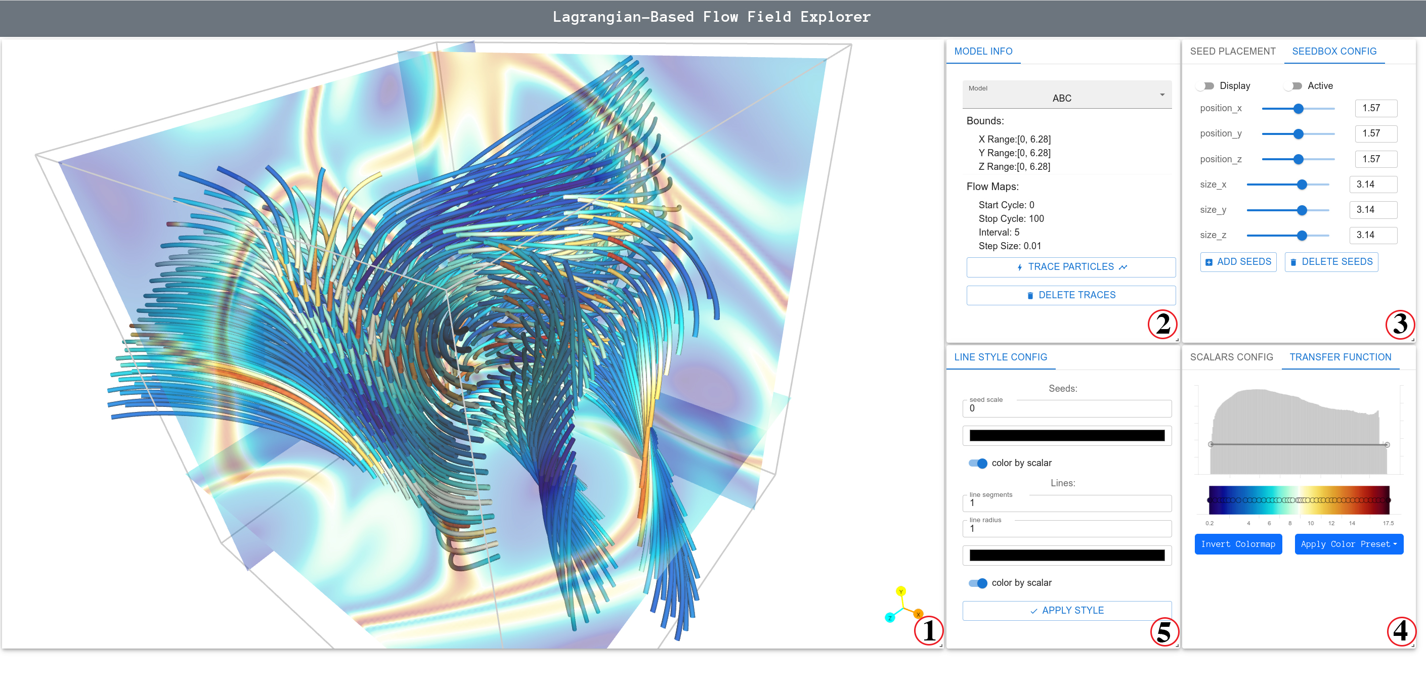
Figure 9: Illustration of our web-based viewer for visualizing inferred pathlines using our pre-trained model in the ABC dataset. The interface includes panels for (1) main display, (2) model loading, data information and particle tracing, (3) seed box configuration, (4) transfer function for scalar field data visualization, and (5) seed and line style configuration.

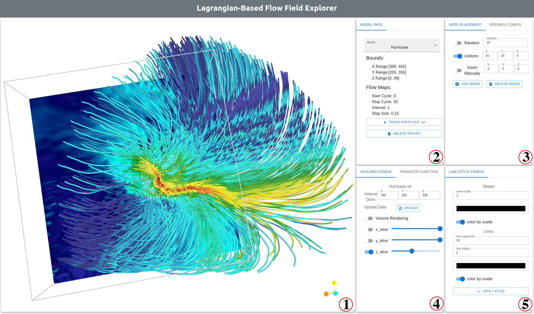
Figure 10: Illustration of our web-based viewer for visualizing inferred pathlines using our pre-trained model in a Hurricane dataset. The interface includes panels for (1) main display, (2) model loading, dataset information and particle tracing, (3) seed placement, (4) scalar field data visualization, and (5) seed and line style configuration.

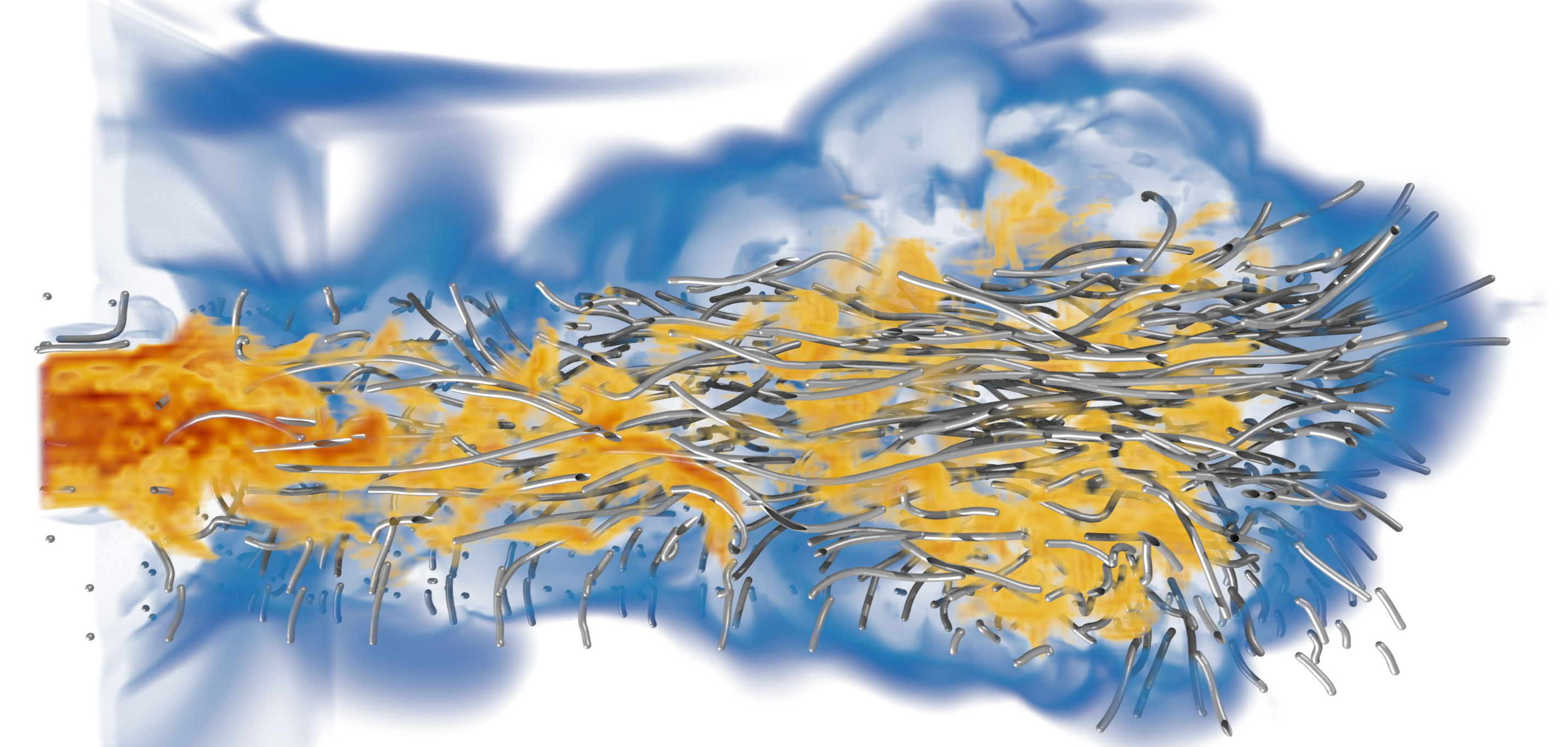
Figure 11: Multi-workflow visualization of the ScalarFlow dataset using our OSPRay-based viewer, which integrates our neural network with the OSPRay renderer. The visualization displays the FTLE as a volume and the pathlines inferred using our neural network. A clipping plane is aligned along the y-axis. The model was trained with the $Lagrangian_{hybrid}$ method. Each pathline encompasses 15 time steps, ranging from time step 135 to time step 150.

4 Conclusion and Future Work

In this paper, we conduct a comprehensive evaluation of a deep learning approach that uses Lagrangian representations to accelerate the post hoc interpolation and visualization of time-varying vector fields.

Our empirical results help identify best practices for using MLP-based models to reconstruct Lagrangian flow maps. Our key findings include:

• Shallow neural networks generally perform better than deep neural networks in reconstructing Lagrangian flow maps;

• The reconstruction errors tend to increase with increased turbulence in flow behaviors. A larger hidden layer (with a higher latent dimension) is more effective than a smaller one for capturing complex flow dynamics;

• The Sinusoidal activation function demonstrates superior performance compared to the ReLU activation function;

• Employing the $Lagrangian_{hybrid}$ method for generating training data effectively minimizes error propagation while preserving domain coverage, in contrast to the $Lagrangian_{long}$ method;

• Model pruning is essential for reducing model size and enhancing the efficiency of the inference process.

By comparing the deep learning approach to the conventional method based on Delaunay triangulation and Barycentric coordinate interpolation, we demonstrate that our approach is at least three times faster on small datasets and over 400 times faster on large 3D datasets. Our method improves interpolation accuracy by three times on average for structured datasets. In terms of storage space, our method reduces memory usage by 46 times for the hurricane dataset, by saving 30 basis flow maps with 1.6 GB storage.

By leveraging the rapid inference and small memory footprint of our MLP model, we provide a web-based viewer to offer an easy way to visualize and explore the post hoc interpolation process. Accessible from any computer regardless of processing capacity, the web-based viewer supports multiple platforms and web browsers. It also provides various seeding strategies and supports both volume and slice representations of other scalar fields, enabling users to select regions of interest and explore them interactively.

When using CUDA-supported devices, our approach can generate pathlines interactively. Inferring 1,000 pathlines with 30 flow maps takes only one second. However, on a low-end device with a single CPU, the inference speed is slower, requiring three seconds to infer 1,000 pathlines with 30 flow maps. Despite the slower performance on low-end devices, interactive pathline generation remains significantly faster than the conventional approach.

Whereas the current parallel scheme for deploying the neural network on the website using a CPU is sub-optimal, we are optimistic that performance can be substantially improved with a more efficient parallel API in the future.

Additionally, we have integrated our neural network into the OSPRay rendering engine to support C++ developers and enable fast, high-fidelity rendering performance. Our integration is general and can be applied to other model architectures with similar tasks. We have made all the source code available on GitHub, allowing users to easily integrate their own neural networks by replacing the trace function.

In addition, our study demonstrates that the proposed neural network, featuring a sinusoidal activation function, significantly improves inference accuracy compared to a prior study [30]. We also investigated the impact of different model architectures on various 2D and 3D datasets, and assessed our model’s ability to handle datasets with increasing flow complexity. Moreover, we evaluated a $Lagrangian_{hybrid}$ training data structure that conceptually combines the $Lagrangian_{long}$ and $Lagrangian_{short}$ methods utilized in [30], ensuring domain convergence while minimizing error propagation’s impact.

While our approach has shown promising results, certain limitations exist. We observed larger errors in unstructured datasets with sparse seeds. To address this, we plan to investigate adaptive seeding approaches that place seeds based on flow features and mesh refinement instead of uniform seeding. Additionally, training the model for large 3D datasets is computationally expensive. We plan to explore ways to reduce training time while maintaining accuracy, such as utilizing transfer learning. Lastly, our model is less effective at inferring long trajectories, especially in complex flow behavior. Improving the model’s capability to handle large-scale datasets is also an area of future research.

References

- [1] A. Agranovsky, D. Camp, C. Garth, E. W. Bethel, K. I. Joy, and H. Childs. Improved Post Hoc Flow Analysis Via Lagrangian Representations. In 2014 IEEE 4th Symposium on Large Data Analysis and Visualization (LDAV), pages 67–75, 2014.
- [2] A. Agranovsky, H. Obermaier, C. Garth, and K. I. Joy. A Multi-Resolution Interpolation Scheme for Pathline Based Lagrangian Flow Representations. In Visualization and Data Analysis 2015, volume 9397, page 93970K, 2015.
- [3] A. S. Ali, A. S. Hussien, M. F. Tolba, and A. H. Youssef. Visualization of Large Time-Varying Vector Data. In 2010 3rd International Conference on Computer Science and Information Technology, volume 4, pages 210–215. IEEE, 2010.
- [4] Y. An, H.-W. Shen, G. Shan, G. Li, and J. Liu. STSRNet: Deep Joint Space-Time Super-Resolution for Vector Field Visualization. IEEE Computer Graphics and Applications, 41(6):122–132, 2021.
- [5] I. Baeza Rojo and T. Günther. Vector Field Topology of Time-Dependent Flows in a Steady Reference Frame. IEEE Transactions on Visualization and Computer Graphics (Proc. IEEE Scientific Visualization), 2019.
- [6] X. Bai, C. Wang, and C. Li. A Streampath-Based RCNN Approach to Ocean Eddy Detection. IEEE Access, 7:106336–106345, 2019.
- [7] A. D. Beck, J. Zeifang, A. Schwarz, and D. G. Flad. A Neural Network based Shock Detection and Localization Approach for Discontinuous Galerkin Methods. Journal of Computational Physics, 423:109824, 2020.
- [8] S. L. Brunton, B. R. Noack, and P. Koumoutsakos. Machine Learning for Fluid Mechanics. Annual Review of Fluid Mechanics, 52:477–508, 2020.
- [9] R. Bujack and K. I. Joy. Lagrangian Representations of Flow Fields with Parameter Curves. In 2015 IEEE 5th Symposium on Large Data Analysis and Visualization (LDAV), pages 41–48. IEEE, 2015.
- [10] J. Chandler, H. Obermaier, and K. I. Joy. Interpolation-Based Pathline Tracing in Particle-Based Flow Visualization. IEEE transactions on visualization and computer graphics, 21(1):68–80, 2014.
- [11] M. V. Da Costa and B. Blanke. Lagrangian methods for flow climatologies and trajectory error assessment. Ocean Modelling, 6(3-4):335–358, 2004.
- [12] L. Deng, Y. Wang, Y. Liu, F. Wang, S. Li, and J. Liu. A CNN-based Vortex Identification Method. Journal of Visualization, 22(1):65–78, 2019.
- [13] C. Dong, C. C. Loy, K. He, and X. Tang. Image Super-Resolution Using Deep Convolutional Networks. IEEE transactions on pattern analysis and machine intelligence, 38(2):295–307, 2015.
- [14] Z. Duo, W. Wang, and H. Wang. Oceanic Mesoscale Eddy Detection Method Based on Deep Learning. Remote Sensing, 11(16):1921, 2019.
- [15] M.-L. Eckert, K. Um, and N. Thuerey. ScalarFlow: A Large-Scale Volumetric Data Set of Real-world Scalar Transport Flows for Computer Animation and Machine Learning. ACM Transactions on Graphics (TOG), 38(6):1–16, 2019.
- [16] B. Elesedy, V. Kanade, and Y. W. Teh. Lottery Tickets in Linear Models: An Analysis of Iterative Magnitude Pruning. arXiv preprint arXiv:2007.08243, 2020.
- [17] A. Fabri and S. Pion. CGAL: The Computational Geometry Algorithms Library. In Proceedings of the 17th ACM SIGSPATIAL international conference on advances in geographic information systems, pages 538–539, 2009.
- [18] G. Fang, X. Ma, M. Song, M. B. Mi, and X. Wang. DepGraph: Towards Any Structural Pruning. arXiv preprint arXiv:2301.12900, 2023.
- [19] J. Frankle and M. Carbin. The Lottery Ticket Hypothesis: Finding Sparse, Trainable Neural Networks. arXiv preprint arXiv:1803.03635, 2018.
- [20] K. Franz, R. Roscher, A. Milioto, S. Wenzel, and J. Kusche. OCEAN EDDY IDENTIFICATION AND TRACKING USING NEURAL NETWORKS. In IGARSS 2018-2018 IEEE International Geoscience and Remote Sensing Symposium, pages 6887–6890. IEEE, 2018.
- [21] G. Froyland and O. Junge. Robust FEM-Based Extraction of Finite-Time Coherent Sets Using Scattered, Sparse, and Incomplete Trajectories. SIAM Journal on Applied Dynamical Systems, 17(2):1891–1924, 2018.
- [22] G. Froyland and K. Padberg-Gehle. A rough-and-ready cluster-based approach for extracting finite-time coherent sets from sparse and incomplete trajectory data. Chaos: An Interdisciplinary Journal of Nonlinear Science, 25(8):087406, 2015.
- [23] H. Gao, L. Sun, and J.-X. Wang. Super-resolution and denoising of fluid flow using physics-informed convolutional neural networks without high-resolution labels. Physics of Fluids, 33(7):073603, 2021.
- [24] T. Günther, M. Gross, and H. Theisel. Generic Objective Vortices for Flow Visualization. ACM Transactions on Graphics (Proc. SIGGRAPH), 36(4):141:1–141:11, 2017.
- [25] L. Guo, S. Ye, J. Han, H. Zheng, H. Gao, D. Z. Chen, J.-X. Wang, and C. Wang. SSR-VFD: Spatial Super-Resolution for Vector Field Data Analysis and Visualization. In 2020 IEEE Pacific Visualization Symposium (PacificVis), pages 71–80. IEEE Computer Society, 2020.
- [26] A. Hadjighasem, M. Farazmand, D. Blazevski, G. Froyland, and G. Haller. A Critical Comparison of Lagrangian Methods for Coherent Structure Detection. Chaos: An Interdisciplinary Journal of Nonlinear Science, 27(5):053104, 2017.
- [27] J. Han, J. Tao, and C. Wang. FlowNet: A Deep Learning Framework for Clustering and Selection of Streamlines and Stream Surfaces. IEEE transactions on visualization and computer graphics, 26(4):1732–1744, 2018.
- [28] J. Han, J. Tao, H. Zheng, H. Guo, D. Z. Chen, and C. Wang. Flow Field Reduction Via Reconstructing Vector Data From 3-D Streamlines Using Deep Learning. IEEE computer graphics and applications, 39(4):54–67, 2019.
- [29] J. Han and C. Wang. TSR-VFD: Generating Temporal Super-Resolution for Unsteady Vector Field Data. Computers & Graphics, 103:168–179, 2022.
- [30] M. Han, S. Sane, and C. R. Johnson. Exploratory Lagrangian-Based Particle Tracing Using Deep Learning. Journal of Flow Visualization and Image Processing, 2022.
- [31] A. Helgeland and T. Elboth. High-Quality and Interactive Animations of 3D Time-Varying Vector Fields. IEEE Transactions on Visualization and Computer Graphics, 12(6):1535–1546, 2006.
- [32] K. Höhlein, M. Kern, T. Hewson, and R. Westermann. A comparative study of convolutional neural network models for wind field downscaling. Meteorological Applications, 27(6):e1961, 2020.
- [33] F. Hong, J. Zhang, and X. Yuan. Access Pattern Learning with Long Short-Term Memory for Parallel Particle Tracing. In 2018 IEEE Pacific Visualization Symposium (PacificVis), pages 76–85. IEEE, 2018.
- [34] J. Jakob, M. Gross, and T. Günther. A Fluid Flow Data Set for Machine Learning and its Application to Neural Flow Map Interpolation. IEEE Transactions on Visualization and Computer Graphics, 27(2):1279–1289, 2020.
- [35] B. Kashir, M. Ragone, A. Ramasubramanian, V. Yurkiv, and F. Mashayek. Application of fully convolutional neural networks for feature extraction in fluid flow. Journal of Visualization, 24(4):771–785, 2021.
- [36] B. Kim and T. Günther. Robust Reference Frame Extraction from Unsteady 2D Vector Fields with Convolutional Neural Networks. In Computer Graphics Forum, volume 38, pages 285–295. Wiley Online Library, 2019.
- [37] J.-Y. Lee and J. Park. Deep Regression Network-Assisted Efficient Streamline Generation Method. IEEE Access, 9:111704–111717, 2021.
- [38] R. Lguensat, M. Sun, R. Fablet, P. Tandeo, E. Mason, and G. Chen. EddyNet: A Deep Neural Network for Pixel-Wise Classification of Oceanic Eddies. In IGARSS 2018-2018 IEEE International Geoscience and Remote Sensing Symposium, pages 1764–1767. IEEE, 2018.
- [39] Y. Li, C. Wang, and C.-K. Shene. Extracting Flow Features via Supervised Streamline Segmentation. Computers & Graphics, 52:79–92, 2015.
- [40] C. Liu, R. Jiang, D. Wei, C. Yang, Y. Li, F. Wang, and X. Yuan. Deep Learning Approaches in Flow Visualization. Advances in Aerodynamics, 4(1):1–14, 2022.
- [41] Y. Liu, Y. Lu, Y. Wang, D. Sun, L. Deng, F. Wang, and Y. Lei. A CNN-based shock detection method in flow visualization. Computers & Fluids, 184:1–9, 2019.
- [42] C. Pheatt. Intel® Threading Building Blocks. Journal of Computing Sciences in Colleges, 23(4):298–298, 2008.
- [43] S. Popinet. Free Computational Fluid Dynamics. ClusterWorld, 2(6), 2004.
- [44] X. Qin, E. van Sebille, and A. S. Gupta. Quantification of errors induced by temporal resolution on Lagrangian particles in an eddy-resolving model. Ocean Modelling, 76:20–30, 2014.
- [45] T. Rapp, C. Peters, and C. Dachsbacher. Void-and-Cluster Sampling of Large Scattered Data and Trajectories. IEEE transactions on visualization and computer graphics, 26(1):780–789, 2019.
- [46] M. P. Rockwood, T. Loiselle, and M. A. Green. Practical concerns of implementing a finite-time lyapunov exponent analysis with under-resolved data. Experiments in Fluids, 60(4):1–16, 2019.
- [47] S. Sahoo and M. Berger. Integration-Aware Vector Field Super Resolution. 2021.
- [48] S. Sahoo, Y. Lu, and M. Berger. Neural Flow Map Reconstruction. In Computer Graphics Forum, volume 41, pages 391–402. Wiley Online Library, 2022.
- [49] S. Sane, R. Bujack, and H. Childs. Revisiting the Evaluation of In Situ Lagrangian Analysis. In EGPGV@ EuroVis, pages 63–67, 2018.
- [50] S. Sane, R. Bujack, C. Garth, and H. Childs. A Survey of Seed Placement and Streamline Selection Techniques. In Computer Graphics Forum, volume 39, pages 785–809. Wiley Online Library, 2020.
- [51] S. Sane and H. Childs. Exploratory Time-Dependent Flow Visualization via In Situ Extracted Lagrangian Rßepresentations. In In Situ Visualization for Computational Science, pages 91–109. Springer, 2022.
- [52] S. Sane, C. R. Johnson, and H. Childs. Investigating In Situ Reduction via Lagrangian Representations for Cosmology and Seismology Applications. In International Conference on Computational Science, pages 436–450. Springer, 2021.
- [53] K. L. Schlueter-Kuck and J. O. Dabiri. Coherent structure colouring: identification of coherent structures from sparse data using graph theory. Journal of Fluid Mechanics, 811:468–486, 2017.
- [54] W. Shi, J. Caballero, F. Huszár, J. Totz, A. P. Aitken, R. Bishop, D. Rueckert, and Z. Wang. Real-Time Single Image and Video Super-Resolution Using an Efficient Sub-Pixel Convolutional Neural Network. In Proceedings of the IEEE conference on computer vision and pattern recognition, pages 1874–1883, 2016.
- [55] V. Sitzmann, J. Martel, A. Bergman, D. Lindell, and G. Wetzstein. Implicit Neural Representations with Periodic Activation Functions. Advances in Neural Information Processing Systems, 33, 2020.
- [56] C. M. Ströfer, J. Wu, H. Xiao, and E. Paterson. Data-Driven, Physics-Based Feature Extraction from Fluid Flow Fields Using Convolutional Neural Networks. Communications in Computational Physics, 25(3):625–650, 2018.
- [57] D. Tatarenkova. Edge Detection and Machine Learning Approach to Identify Flow Structures on Schlieren and Shadowgraph Images. 2020.
- [58] I. Wald, G. P. Johnson, J. Amstutz, C. Brownlee, A. Knoll, J. Jeffers, J. Günther, and P. Navrátil. OSPRay-A CPU Ray Tracing Framework for Scientific Visualization. IEEE transactions on visualization and computer graphics, 23(1):931–940, 2016.
- [59] C. Wang and J. Han. DL4SciVis: A State-of-the-Art Survey on Deep Learning for Scientific Visualization. IEEE Transactions on Visualization and Computer Graphics, 2022.
- [60] Y. Wang, L. Deng, Z. Yang, D. Zhao, and F. Wang. A Rapid Vortex Identification Method Using Fully Convolutional Segmentation Network. The Visual Computer, 37(2):261–273, 2021.
- [61] T. B. L. Yi. CNN-based Flow Field Feature Visualization Method. International Journal of Performability Engineering, 14(3):434, 2018.