Optimal coordination in Minority Game: A solution from reinforcement learning
Abstract
Efficient allocation is important in nature and human society where individuals often compete for finite resources. The Minority Game is perhaps the simplest model that provides deep insights into how human coordinate to maximize the resource utilization. However, this model assumes the static strategies that are provided a priori, failing to capture their adaptive nature. Here, we turn to the paradigm of reinforcement learning, where individuals’ strategies are evolving by evaluating both the past experience and rewards in the future. Specifically, we adopt the Q-learning algorithm, each player is endowed with a Q-table that guides their decision-making. We reveal that the population is able to reach the optimal allocation when individuals appreciate both the past experience and rewards in the future, and they are able to balance the exploitation of their Q-tables and the exploration by randomly acting. The optimal allocation is ruined when individuals tend to use either exploitation-only or exploration-only, where only partial coordination and even anti-coordination are observed. Mechanism analysis reveals that a moderate level of exploration can escape local minimums of metastable periodic states, and reaches the optimal coordination as the global minimum. Interestingly, the optimal coordination is underlined by a symmetry-breaking of action preferences, where nearly half of the population choose one side while the other half prefer the other side. The emergence of optimal coordination is robust to the population size and other game parameters. Our work therefore provides a natural solution to the Minority Game and sheds insights into the resource allocation problem in general. Besides, our work demonstrates the potential of the proposed reinforcement learning paradigm in deciphering many puzzles in the socio-economic context.
I 1. Introduction
Scarcity is the fundamental property in most economic problems Samuelson and Nordhaus (2005), where the society is incapable to fulfill the ever-increasing wants and needs in a world of finite resource, and is the root of most wars. The efficient allocation of resource thus becomes a core concern of economy. However, this issue is conceptually different from the commonly seen optimization problems, where a single objective function can be defined to be optimized; instead it is a Paretto problem Hwang and Masud (2012), the improvement of one’s well-being is accompanied with the benefit deterioration of someone else since individuals have typically conflicting goals.
A remarkable insight in Economics is that markets themselves in most of time are able to reach such an optimal allocation. This comes from the self-organization of markets, and is well explained according to Adam Smith Smith (2003) in his famous quote “It is not from the benevolence of the butcher, the brewer, or the baker, that we expect our dinner, but from their regard to their own interest.” The key question to be addressed here is that, in the pursuit of self-interests for individuals, how the optimal allocation is achieved for the the population as a whole? This is also the key question behind the market efficiency. As the mainstream theory in economy, the general equilibrium theory Arrow (1974) has provided important insights into the properties of optimal allocation when reached, yet it fails to understand how the optimal allocation is achieved and under what conditions.
Important progress comes from the complexity science, which is initialized by the EI Farol bar problem (EFBP) proposed by Brian Arthur Arthur (1994). In this problem, a fixed number of residents face the question of whether or not go to the bar. If the bar is not crowded, as measured by the capacity of bar like the number of seats, one wins if the player decides to attend. If the bar is crowded, one wins if stays at home. Each person makes decisions based on the attendance records, and Arthur showed how the equilibrium can be reached by inductive thinking Arthur (1994).
Inspired by the EFBP, the Minority Game (MG) introduced by Challet and Zhang Challet and Zhang (1997); Challet et al. (2005) mainly focuses on fluctuations around the equilibrium, and provides possibly the simplest formulation to understand the competition for the finite resource. The scenario can be simplified as follows: an odd number of agents repeatedly choose to go two rooms, those who are within the less crowded room win, the other lose. The system is intrinsically frustrated, because no solution can satisfy everyone. A fundamental difference from the EFBP is that the MG focuses on fluctuations around the equilibrium, a smaller fluctuation means better utilization of the resource. Specifically, in the scheme proposed in Ref. Challet and Zhang (1997), each agent is assigned with a recipe of lookup tables based upon the historic record sampling from a common strategy pool, the strategy with a higher score is reinforced to adopt. If is large, the agents would necessarily employ many similar strategies, the population shows the herding behaviors; In the opposite case, their strategies virtually never meet, where each agent behaves independently and randomly; Somewhere in between, the fluctuation around the equilibrium is minimized, meaning the more resources are utilized.
To reveal mechanism behind the coordination based upoon the MG, there are two lines of research Marsili et al. (2000); Marsili and Challet (2001); Hart et al. (2001); Chakraborti et al. (2015); Paczuski et al. (2000); Huang et al. (2012); Li et al. (2000); Liaw et al. (2007); Dyer et al. (2008); Zhang et al. (2013). One line, primarily developed by statistical physicists, utilizes replica calculus combining with partition function Marsili et al. (2000); Marsili and Challet (2001); Hart et al. (2001) or generating functionals Heimel and Coolen (2001); De Martino and Galla (2011); Galla et al. (2003) to establish a connection between the Minority Game and nonequilibrium phase transitions Chakraborti et al. (2015); Galla and De Martino (2008); Bottazzi et al. (2002). Building upon these studies, numerous modifications and extensions of the Minority Game also have been invented and thoroughly investigated after taking into account factors such as payoffs Li et al. (2000); Liaw et al. (2007), strategy distributions Coolen and Shayeghi (2008); Garrahan et al. (2001) and learning algorithms Montague et al. (2006); Catteeuw and Manderick (2011), etc. The other line applies Boolean game dynamics, assuming each agent possess local information about it interacts with, enabling the agent to respond accordingly for the sake of entering the minority group Paczuski et al. (2000); Huang et al. (2012); Dyer et al. (2008); Zhang et al. (2013, 2016); Zhou et al. (2005). However, part of the success is due to the handcrafted rules. A recipe by design in Ref. Challet and Zhang (1997) is composed of fixed number of strategies, but it’s hard to expect in the real life that players have the same number of rules sampled from a common pool. Within the recipe, the strategies themselves remain unchanged, which also fail to capture the adaptive nature of strategies in the real world.
Here, we turn to the paradigm of reinforcement learning to provide a different solution to the MG. As one main category of machine learning algorithms, reinforcement learning specializes the decision-making in complex scenarios, and has shown its great potential in autonomous driving, natural language processing, gaming Silver et al. (2016) etc. In fact, the design of RL was motivated by the behavior modes observed across different species and has a solid foundation in neuroscience Lee et al. (2012); Rangel et al. (2008). The paradigm of RL is supposed to well suited to the study of the evolution of human behaviors, like the resource allocation problem here. Recently, researchers start to combine the RL with the evolutionary game theory to understand the cooperation Zhang et al. (2020a); Song et al. (2022); Ding et al. (2023), the resource allocation Andrecut and Ali (2001a); Zhang et al. (2019a), trust Zheng et al. (2023), and other collective behaviors in complex systems Zhang et al. (2020b); Tomov et al. (2021); He et al. (2022); Shi and Rong (2022). These early efforts have released the potential of RL in deciphering the puzzles in social and economic contexts, though the full unleash of its power is so yet to come.
Actually, a few previous studies have combined RL to study the MG. Ref. Andrecut and Ali (2001b) presents an earliest attempt by applying Q-learning to the MG, where the herding effect is suppressed. Similar observations are made in a larger population in Ref. Zhang et al. (2019b), where they also adopt Q-learning. There, they claimed that the population evolves toward the optimal allocation state, but with persistent large fluctuations. These fluctuations are so large, it’s not convincing that’s a satisfactory solution to the MG problem. Till now, the key questions that how whether the optimal allocation is learnable by RL, and what insights RL can provide to the solution of the MG still remain open.
In this study, we propose a reinforcement learning paradigm Sutton and Barto (2018) to perfectly solve the Minority Game, where individuals revise their strategies by evaluating the long-term returns through accumulated experience. Specifically, we adopt an Q-learning algorithm Watkins (1989, 1992), where each agent has a Q-table in hand to guide one’s decision-making. Besides, there is a temperature-like parameter controlling the tradeoff between the exploitation of the past experience and the random exploration. Surprisingly, within the proposed framework, we reveal that a rich spectrum of collective modes of the aggregate are observed, including partial coordination, optimal coordination, anti-coordination. Physically, in the exploitation-only scenario, the population is prone to be trapped in the local minimums in the form of periodic states. The presence of exploration acts as perturbations helping to escape the local minimums, an appropriate level of exploration is able to balance the two that the optimal coordination as the global minimum is reached. However, too much exploration ruins the stability of optimal coordination and could lead to anti-coordination. We also examine the impact of the learning parameters on different collective modes.
II 2. Model
Let’s adopt the El Farol bar as our context. The problem of the Minority Game is then rephrased as follows: Given an odd number of players, say , in each round each has to independently make a binary choice – go or not go to the bar. For simplicity, the bar capacity is assumed . Thus, the winners are those who end up at the minority side, and each gets 1 point. Losers are at the majority side, get zero.
| Go () | Not go () | |
|---|---|---|
| 0 | ||
| 1 | ||
| 2 | ||
| 3 | ||
| … | … | … |
| N |
Instead of distributing ready-made strategies to the individuals as in Challet and Zhang (1997), each has to learn a policy. Specifically, they adopt a model-free and value-based reinforcement learning – the Q-learning algorithm Watkins (1989, 1992). Within this algorithm, each player has a Q-table in mind that directs the action choice of going or not going to the bar, see Table 1. The states are the number of people went to the bar in the last round denoted as , and the action set includes two binary choices , corresponding to going or not going to the bar respectively. The elements in Table 1 is the value function, measuring the value of action within in the given state . The action with a larger value of is supposed to be more preferred within the given state , according to the Q-learning algorithm.
The evolution follows a synchronous updating scheme, where every single round includes two elementary processes – the game and learning processes. Without loss of generality, all Q values in the table are set to be zero, mimicking the status of no preference at the very beginning when entering in a new environment. In round , the first process is playing the Minority Game. To balance the trail-and-error exploration and the exploitation of Q-table, the softmax manner is employed by the player to choose an action, i.e. the probability of action being chosen for player is given by
| (1) |
where is the state of player , and represents the number of actions available, which is 2 in our case. Note that in the Minority Game, the states are identical for all players, i.e. , is the number of people went to the bar at the end of round . The parameter is a temperature-like quantity that controls the trade-off between the exploration and exploitation events. While the exploitation is to follow the guidance of the Q-table summarized from the past experience, the exploration goes beyond the Q-table by trying random actions to explore the environment. At a low temperature , the action with a larger Q-value is probably to be chosen, whereas a random action choice is more likely to be selected for the opposite scenario. In the extreme case of , players strictly choose the action with the larger value, i.e. only exploitation of the Q-table. In the other extreme of , players essentially make random choice of the two action irrespective of their Q-values, i.e. only the exploration is conducted. The ideal policies however generally require a balance of the two, the optimal temperature is supposed to be located in between the two extreme values. Once every player makes the choice of going or not going to the bar, the winning side can then be determined by comparing the total number of people going to the bar with the capacity , and those who are within the minority get one point as the reward, otherwise get nothing.
To this end, the evolution enters into the second process, where all players need to update their Q-tables as learning. Specifically, for player , the element in its Q-table is updated as follows
| (2) |
where and are respectively the state and the action taken at round , is the state for the next round , is the reward in this round, equal 1 or 0. is the learning rate that determines the evolution pace of the Q-table, a small corresponds to a slow evolution, the old value is largely kept, the historical experience is well preserved. A large value of can be instead interpreted as being forgetful. is the discount factor, determines the importance of future rewards, as the associated term gives the expected value in the new round . A larger value of means that players pay more attention to the future’s guidance, having a long-term vision. After every player completes their learning processes, the evolution of round is then finished. The two processes repeats until the population reach equilibrium or the evolution time reaches the desired long durations. The evolution protocol is summarized in Fig. S1 in SM for clarity.
In our study, we fix and the bar capacity in most of our studies if not stated otherwise. To measure the degree of utilization of bar, we define as the volatility Challet et al. (2005), where is the variance of around the capacity , i.e. . The smaller is the volatility, the better used is the bar. If , the bar maximizes its utilization as , and nearly as much as half of people are on the winning side in each round. As a benchmark, when individuals randomly choose to go or not to go to the bar, e.g. by flipping the coin, is expected Challet et al. (2005).
A key question for individuals in this RL paradigm is how to properly handle the exploration-exploitation dilemma Sutton and Barto (2018). On one hand, the scenario of exploitation-only strategy may fall into suboptimal solution without sufficiently exploring the untried possibilities; on the other hand, the individuals in the case of exploration-only neglect the lessons drawn from the past experiences, they decide whether go to the bar by simply flipping the coin, they certainly also fail to reach the optimal coordination. Therefore, how to balance the two is the primary question to be addressed in our study.
III 3. Results
We first report the impact of the temperature on the game evolution to examine the exploration-exploitation dilemma, where three qualitatively distinct phases are observed, as shown in Fig. 1.
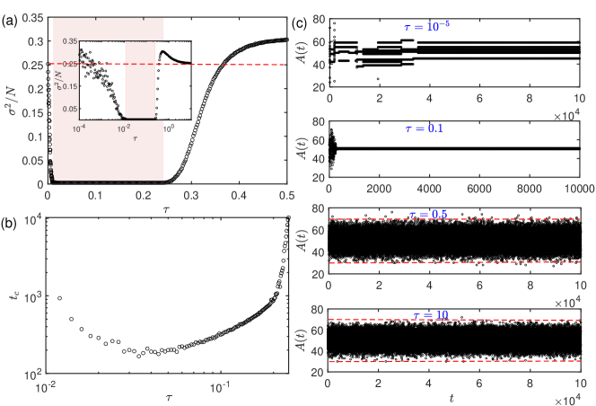
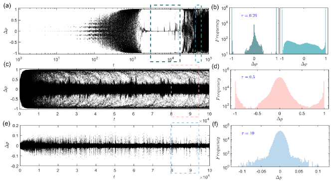
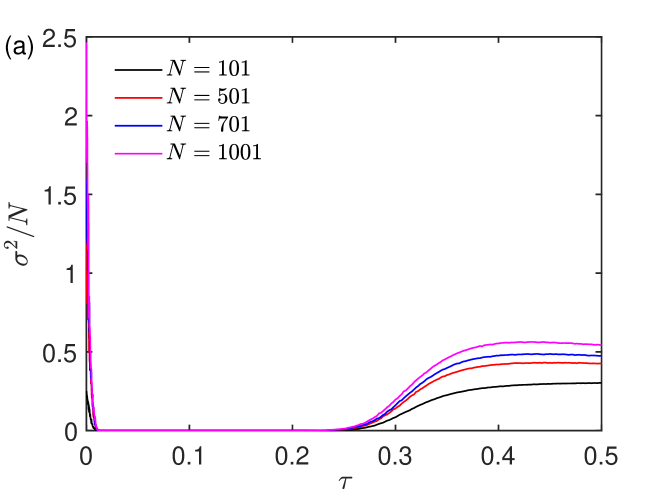
Fig. 1(a) shows the results of the volatility as a function of the temperature , which reveals an non-monotonic dependence as expected. As individuals are inclined to exploitation-only (), the volatility is as large as being around 0.25, meaning that the coordination is failed and as bad as the benchmark scenario. As increases, the trail-and-error explorations are on site, the fluctuations around the bar capacity are gradually reduced, meaning that the population start to learn how to coordinate to improve the utilization of bar. The outcome is, however, not optimal, thus can be termed as the partial coordination (PC) state. Surprisingly, as continues to increase (), the population enters into the optimal coordination (OC) state, where the attending number fluctuates around in the 50-51 manner, the volatility has reached its minimum, the optimal scenario one can expect. Further increase in (), however, the volatility starts to rise, and there is a region where , meaning the coordination is even worse than the benchmark scenario. We term this phenomena as anti-coordination (AC). Finally, as individuals tend to be exploration-only (), the volatility is approximately 0.25, equal to the benchmark value as expected. Detailed inspection shows that the AC scenario () is even worse where the distribution of the attending number is wider.
Typical time series are shown in Fig. 1(c), which respectively show the case of exploitation-only, OC, AC, and the exploration-only case from the top to the bottom. In the case of exploitation-only (), the number of people going to the bar evolve into some meta-stable periodic states, but obviously this state is not satisfactory as the value of deviates considerably from the bar capacity . In the case of optimal coordination (), the number of going to bar strictly fluctuate between the two cases of 50 and 51, the best solution one can expect in the setup of MG. In the other extreme (), the evolution of become quite random and is also unsatisfactory as expected.
Even though the solutions in the OC region () are all the same in the end, there the transient time differs for different temperature . Fig. 1(b) shows that there exists the shortest converging time towards the optimal solution at around . With this temperature, the population is able to reach the OC state within the shortest time.
Overall, the observations in Fig. 1 show that the population fails to coordinate in either extreme of exploitation-only or exploration-only, but they benefit from the trade-off between the exploration and exploitation, and the optimal scenario emerges in their dilemma.
IV 4. Dynamical mechanism
To understand how individuals succeed to coordinate in some cases and why fail in some other cases, we turn to the dynamical mechanism analysis in the this section. We fix the two learning parameters and in this section, where individuals appreciate both their historical experience and returns in the future.
IV.1 A. Exploitation-only
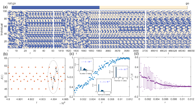
We first focus on the exploitation-only case (), where the decision-making is strictly guided by one’s Q-table. A typical spatial-temporal pattern within four different stages is shown in Fig. 2(a). It shows that, after the transient the population enters into some periodic states (the leftmost panel), but these periodic states are often metastable, they become destabilized and the system evolves into a new one (the two panels in the middle). This process repeats until a stable periodic state is reached (the rightmost panel).
The dynamical mechanism behind this evolution is caused by the “stubbornness” of individuals due to the small value of , which makes the population prone to fall into some metastable states. To be specific, let’s consider individual at round , after it chooses action , it falls into two situations:
(i) If happens to be on the winning side, the reward is obtained, this immediately makes the Q-value of the corresponding action larger than the opposite action denoted as , i.e. . This difference makes the individual firmly choose the action when the system enters the same state next time, as the small value of is able to turn a small advantage in the Q-value into a strong preference in the action selection, as shown in Eq. (1).
(ii) Otherwise, individual is on the losing side with . In this situation, there are two different scenarios: (1) the new state has not been experienced before, or the new state has been experienced but with two values still being zero; in both cases, there the expected value . Therefore , no preference is formed within the state . (2) But if the new state was experienced and individual got positive rewards, , this contributes to the increase in , the action is thus preferred next time when the system is within the state .
In the extreme of , a small difference between and yields a strong preference in action selection, one stubbornly chooses the action with the larger Q-value until this difference vanishes. Since the population is of finite size, a cycle of the is easily formed by evolution, i.e. the population falls into some periodic states.
Within such a periodic state, each individual has an clear preference for each state at the early stage after the cycle is formed, the evolution becomes almost deterministic. But why some periodic states become unstable? The reason lies in the fact that for individual , even though the preferences are formed for each state within this circle, but if no positive reward is obtained through the whole circle, the preference is weakened gradually for the decay relationship . Finally, the individual randomly chooses an action between the two actions when the two Q values become very close (i.e. ), and the stability of the cycle is broken and the cycle collapses, where a turbulence-like pattern or a quick arrangement may be seen as shown in the second and third snapshots in Fig. 2(a).
A periodic state is stable only when all individuals have at least one positive reward through the whole circle, whereby the expected value in each state within the cycle, and all the preferences are strengthened to confront their decay. Such a stable state is seen in the last snapshot in Fig. 2(a). The corresponding time series of the attending number is shown in Fig. 2(b), which is a periodic state with period-6.
IV.2 B. Partial coordination
As the temperature increases, the exploration events are engaged, the evolution to the periodic states becomes harder and harder. An evidence is that the transition time needed from one periodic state to another is increased [see Fig. SX in SM]. By contrast, the increase in prompts the probability towards the optimal coordination state. Fig. 2(c) shows that the probability that the system finally evolve into the OC state as a function of with . We can see that even in the extreme case of , there is already a probability around that the system falls into the OC state; as is creased, this probability continually increases and approaches 1 as . Detailed statistical analysis confirms this observation, as the probability density function (PDF) of the number of states in the final stable states show some relative long periodic states (such as periodic–7, 8) abound for small (e.g. ), but they become fewer (e.g. ), and almost disappear as becomes large (e.g. ), where the OC state dominates. But notice that, the OC state is not a periodic state, the randomly switches between and .
As a consequence, the resulting volatility also declines as the increase of in this range, and approaches the minimum 0.0025 for the OC state. This is due to the deviations of those periodic states from the capacity , compared to the scenario in the OC state. The shortened error bars indicate the decrease in the number of metastable states.
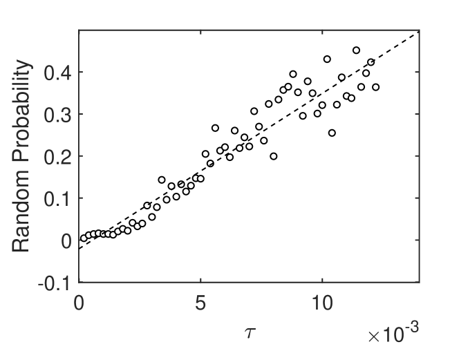
According to Eq. (1), increasing increases the probability of choosing the action with a smaller Q-value, which can be interpreted as that individuals become less stubborn, as they deviate the guidance of their Q-tables more frequently. As increases, this deviation probability increases, as shown in Fig. 3. From the physics point of view, those periodic states are suboptimal solutions and can be taken as local minimums in the phase space, and the temperature acts as the perturbation. With a small value of , the state of population is easily trapped in local minimums. Increasing , the perturbations destablize their stay in those local minimums, and the system escapes from local minimums and becomes more likely to fall into the global minimum — the OC state. As the temperature , none of these periodic states is stable and the system falls into the OC state in all realizations. An evolving pattern is shown in SM (Fig. SX in section X), where one can intuitively see the formation of OC state and the temporal evolution of the associated fluctuations.
IV.3 C. Optimal coordination
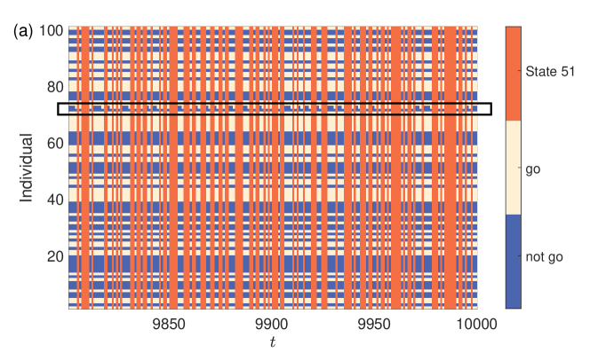
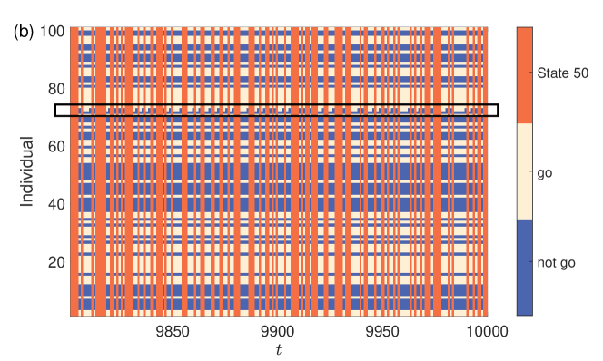
But how the OC states of the population are orchestrated at the individual level? Our analysis shows that within either state or , there is a symmetry-breaking in two action choices, the population is divided into two subgroups: 50 individuals are determined to go to the bar, 50 choose not to go, the rest one is irresolute who randomly switches between the two choices. This can be seen from the action patterns within the OC state shown in Fig. 4, where the system has reached the stationary state
Fig. 4(a) shows the case within the state . We can see that all individuals except the one labeled “71” in this example keep consistent choice of action. Specifically, individuals stick to going to the bar, the other ones not going to the bar. This leaves an awkward situation for individual-71: whichever side it chooses, the chosen side becomes 51 and is thus the losing side. The pathetic fact for individual-71 is that the same evolution repeats within the state that it always gets zero reward. The associated two Q-values , the two actions are selected with an equal probability, which explains the random choice in the OC state. For the rest individuals, the expected reward within for each, which in turn strengthens their preferences with in their Q-tables.
Similar observations are made within the state , where individual-71 still acts the pathetic one, see Fig. 4(b). Note that, the emergence of this pathetic individual in either state is purely by chance, whose preference is the least determined at the early stage of evolution. This makes the individual who restlessly switches its actions, and the continuous loss strengthens one’s indecisiveness. By contrast, the continuing return for the rest strengthens their preferences in the two states. Therefore, it is the pathetic individual who determines which of the two subgroups win and guarantees the frozen state of the rest, and this is crucial for the stability of the OC state. It is worthy noting that before reaching this stationary state, the pathetic individuals are generally different within the two states, their competition turns the less rewarded one into the pathetic individual in both states. This nontrivial dynamical process is discussed in Sec. SX in SM.
Interestingly, in an early work Whitehead et al. (2008), where the EFBP is revisited by a RL algorithm Erev and Roth (1998), this work predicted with a mathematical proof that the population is going to subdivided into two groups: those who invariably go to the bar and those who never do. Our work thus confirms the sorting phenomenon and provides an explanation, though the model details are different.
IV.4 D. Anti-coordination
As the temperature further increases, the OC state is ruined and the anti-coordination may arise. Here we focus on how the OC state is destabilized and the dynamical mechanism behind the emergence of AC state.
Fig. 5(a) provides an example of evolution with the temperature , slightly larger than the upper threshold 0.24 of the OC state. As can be seen, the preference characterized by shows that the population initially of no preference self-organize into the three subgroups — 50 individuals with , 50 with , and 1 with after around steps. The OC state is reached, where the corresponding PDF of is shown in the left panel of Fig. 5(b). However, this state becomes destabilised as time goes by as follows: the individuals in the two subgroups are not so determined to go or not to go to the bar for the given temperature , and they deviate by chance the actions suggested by their Q-tables. Once such action deviation occurs, this could lead to a cascade of action deviation for the rest, including the pathetic player, who may become stick to one of the two choices for a given state. As more and more action deviations occur, the average reward for the originally two subgroups cannot be guaranteed, and the individuals these two subgroups becomes even less determined. These again lead to more deviations, and finally the choice consistence of two subgroups collapses. This is what we see in the latter stage of evolution in Fig. 5(a), and the PDF shows a blurred distribution between the two peaks [the right panel of Fig. 5(b)]. Though two preferences suggested by the two peaks are still very strong.
As further increases to , the OC state is not reachable at all, and AC state could be seen. This is because the required self-organization fails, as observed in Fig. 5(c). The corresponding PDF of shown in Fig. 5(d) shows that the peak around zero dominates, meaning that most of actions taken are of weak preference. But, the two peaks around are still present and comparable to the middle one. Although PDF in Fig. 5(d) is statistically symmetrical regarding going or not going to the bar, there is a time-scale separation in weak and strong preference cases that will introduce a bias in superposition. Specifically, the preference switching for these determined has much longer time scale than the weak preference cases, see Fig.SX in SM. Given the slow-varying bias, the superposition of the aggregate of the weak determined actions results in a wider distribution of . This thus leads to an enhanced volatility compared to the purely weak determined actions and explains the emergence of anti-coordination.
Obviously, the occurrence of anti-coordination is different from the herding effect as observed in the original MG model Challet and Zhang (1997); Challet et al. (2005). The herding is the consequence of adopting the same lookup tables by some people, while the AC here is due to the strong preference in some states, and time scale separation for the preference switching, the attending number of the slow switching aggregate introduce a bias to the rest of fast switching aggregate.
V 5. Phase diagram
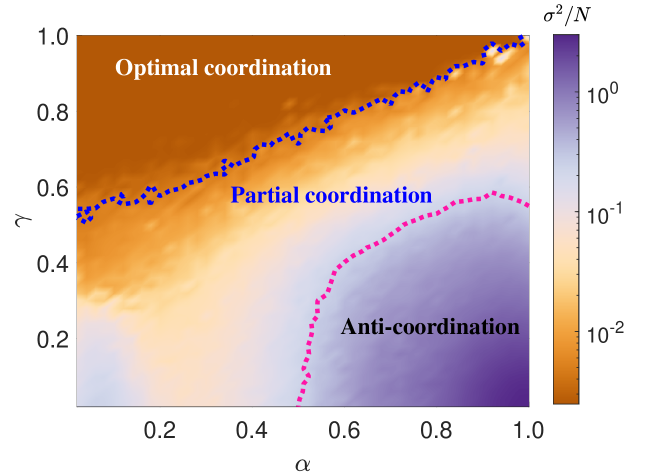
To systematically examine the impact of the parameters in Q-learning, we provide the phase diagram of the volatility in the parameter domain, as shown in Fig. 6. It shows that the domain can be divided into three regions: optimal coordination, partial coordination, and anti-coordination.
As seen, the OC region typically corresponds the combination of small and large , where the individuals both care about the historical experience and the long-term return. The opposite scenario with large and small correspond to the anti-coordination outcome where the volatility , the interactions among individuals through Q-learning bring the herd effect as discussed in Sec. 3D.The PC state locates between these two regions, where the volatility is larger than the value of optimal coordination but smaller than the benchmark value 0.25.
These observations are in line with our exception. Because once individuals are forgetful (with a large ), few lesson can be drawn from the history, the Q-learning loses its strength. With the premise of a small learning rate , the larger the discount factor is, the stronger guidance there is from the future, which generally better directs the system into a desired outcome as indeed seen in Fig. 6. The dependence of performance is qualitatively same as the previous work in Ding et al. (2023); Zheng et al. (2023), where high prevalence of trust or cooperation are observed when the Q-learning individuals are of small and large .
VI 6. Robustness
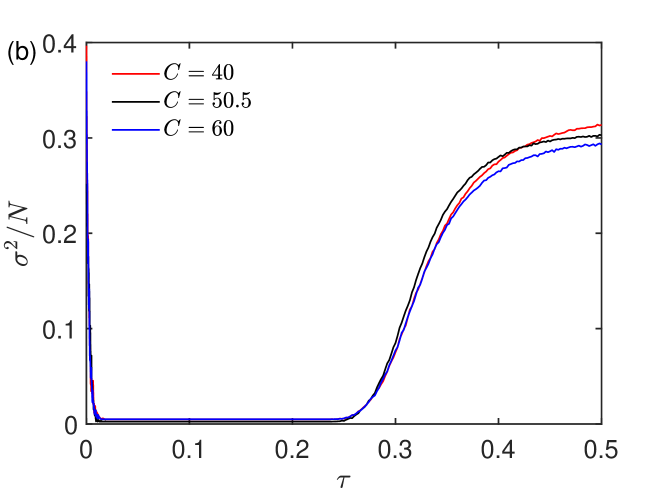
In fact, the observations made in population size and the bar capacity can be generalized in the different population sizes and bar capacities. Figure. 7(a) shows that when we increase the population size up to , and the phase transition and the regions for different phases remains almost unchanged. Similar robustness is seen when the bar capacity is varied, when the population size is fixed at in Figure. 7(b). We see the capacity of bar is not necessarily to be half of the population, as the setup of the of the Minority Game often assumes.
Furthermore, these observations can even be seen in an even number of population , where is a integer and the bar capacity . In this case, we need to make a rule that which side wins when the half-split case of is seen. We find that in either case (going to the bar or not-going to the bar wins), the observations made in the above odd number scenario remains the same. In particular, the orchestration of OC state is slightly different, where the two frozen subgroups are not strictly of the same size anymore. One pathetic player emerges that always be the loser, of the rest are determined to go (or not to go), players choose the opposite. A case for is shown in Sec. X in SM.
VII 7. Discussion
In summary, we provide a solution to the resource allocation problem within the reinforcement learning paradigm. Specifically, we adopt a Q-learning algorithm to solve the Minority Game, where each player is empowered with an evolving Q-table that guides one’s move. We reveal that the aggregate could evolve into different phases, depending on the trade-off between their exploitation of Q-tables and the exploration. With insufficient exploration, the population is prone to fall into periodic states, many of these periodic states are metastable and the coordination is suboptimal. With too much exploration on the other hand, the coordination is also bad since the individuals act just like by flipping the coin. To our surprise, when the trade-off of the two is balanced, we observe the emergence of optimal coordination, where the volatility is minimized around the capacity. Interestingly, there is a symmetry-breaking within the population’ preference, where nearly half of people invariably go to bar, the other half never do for the given state, and one ever-losing/irresolute individual who restlessly switches its action. Between the case of optimal coordination and exploration-only, there is an anti-coordination phase where the coordination is even worse than the flipping coin manner, due to the bias introduced by those individuals with a strong preference in some states.
As the scarcity is an intrinsic property of our world, the proposed paradigm provides a novel perspective to solve the resource allocation problems in our society. Our findings suggest that by integration of the past experience, the reward at present and in the future, amazingly the population is able to reach the optimal coordination during the process where the individuals seek to maximize their accumulate rewards. This reconciles the individuals’ self-interests and the resource allocation at the population level. Our results thus may also provide a plausible solution to the efficient market assumption Samuelson and Nordhaus (2005), and its failure may also be attributed to the balance-breaking of trade-off between exploitation and exploration.
Compared to the original scheme in Ref. Challet and Zhang (1997); Challet et al. (2005), our work shows that the Q-table as the policy is learnable, and is coevolving with the environment. In particular, to achieve the optimal coordination, their Q-tables self-organize into structured sorting. It is the policy heterogeneity that makes the optimal coordination possible. This heterogeneity spontaneously emerges in our Q-learning scheme but needs to be artificially tuned in Ref. Challet and Zhang (1997); Challet et al. (2005). Though, we have’t not yet develop any theoretic treatment as those for the original scheme Challet et al. (2005), and we leave to the future. Even so, the stability dependence of periodic states on the temperature-like parameter suggests the energy landscape theory Wales (2018); Fang et al. (2019) may be a good starting point.
Although the proposed paradigm provides a satisfactory solution to the allocation problem in Minority Game, we have no idea that to what extend the revealed mechanism works for realistic scenarios. We call for the behavioral experiments to be carried out to validate or falsify our findings and to further compare the realistic processes to the rich spectrum of dynamics uncovered here.
VIII Acknowledgments
This work is supported by the National Natural Science Foundation of China [Grants Nos. 12075144,12165014]. ZGZ is supported by Excellent Graduate Training Program of Shaanxi Normal University [Grants No. LHRCTS23064].
References
- Samuelson and Nordhaus (2005) P. Samuelson and W. Nordhaus, Economics (18th edition) (McGraw-Hil Education, 2005).
- Hwang and Masud (2012) C.-L. Hwang and A. S. M. Masud, Multiple objective decision making—methods and applications: a state-of-the-art survey, Vol. 164 (Springer Science & Business Media, 2012).
- Smith (2003) A. Smith, The wealth of nations [1776] (Bantam Classics, 2003).
- Arrow (1974) K. J. Arrow, The American Economic Review 64, 253 (1974).
- Arthur (1994) W. B. Arthur, The American Economic Review 84, 406 (1994).
- Challet and Zhang (1997) D. Challet and Y.-C. Zhang, Physica A: Statistical Mechanics and its Applications 246, 407 (1997).
- Challet et al. (2005) D. Challet, M. Marsili, and Y. C. Zhang, Minority Games: Interacting agents in financial markets (Oxford Finance Series, 2005).
- Marsili et al. (2000) M. Marsili, D. Challet, and R. Zecchina, Physica A: Statistical Mechanics and its Applications 280, 522 (2000).
- Marsili and Challet (2001) M. Marsili and D. Challet, Physical Review E 64, 056138 (2001).
- Hart et al. (2001) M. Hart, P. Jefferies, P. Hui, and N. Johnson, The European Physical Journal B-Condensed Matter and Complex Systems 20, 547 (2001).
- Chakraborti et al. (2015) A. Chakraborti, D. Challet, A. Chatterjee, M. Marsili, Y.-C. Zhang, and B. K. Chakrabarti, Physics Reports 552, 1 (2015).
- Paczuski et al. (2000) M. Paczuski, K. E. Bassler, and Á. Corral, Physical Review Letters 84, 3185 (2000).
- Huang et al. (2012) Z.-G. Huang, J.-Q. Zhang, J.-Q. Dong, L. Huang, and Y.-C. Lai, Scientific reports 2, 703 (2012).
- Li et al. (2000) Y. Li, A. VanDeemen, and R. Savit, Physica A: Statistical Mechanics and its Applications 284, 461 (2000).
- Liaw et al. (2007) S.-S. Liaw, C.-H. Hung, and C. Liu, Physica A: Statistical Mechanics and its Applications 374, 359 (2007).
- Dyer et al. (2008) J. R. Dyer, C. C. Ioannou, L. J. Morrell, D. P. Croft, I. D. Couzin, D. A. Waters, and J. Krause, Animal Behaviour 75, 461 (2008).
- Zhang et al. (2013) J.-Q. Zhang, Z.-G. Huang, J.-Q. Dong, L. Huang, and Y.-C. Lai, Physical Review E 87, 052808 (2013).
- Heimel and Coolen (2001) J. Heimel and A. Coolen, Physical Review E 63, 056121 (2001).
- De Martino and Galla (2011) A. De Martino and T. Galla, New Mathematics and Natural Computation 7, 249 (2011).
- Galla et al. (2003) T. Galla, A. Coolen, and D. Sherrington, Journal of Physics A: Mathematical and General 36, 11159 (2003).
- Galla and De Martino (2008) T. Galla and A. De Martino, Journal of Physics A: Mathematical and Theoretical 41, 324003 (2008).
- Bottazzi et al. (2002) G. Bottazzi, G. Devetag, and G. Dosi, Simulation Modelling Practice and Theory 10, 321 (2002).
- Coolen and Shayeghi (2008) A. Coolen and N. Shayeghi, Journal of Physics A: Mathematical and Theoretical 41, 324005 (2008).
- Garrahan et al. (2001) J. Garrahan, E. Moro, and D. Sherrington, Quantitative Finance 1, 246 (2001).
- Montague et al. (2006) P. R. Montague, B. King-Casas, and J. D. Cohen, Annu. Rev. Neurosci. 29, 417 (2006).
- Catteeuw and Manderick (2011) D. Catteeuw and B. Manderick, in International Workshop on Adaptive and Learning Agents (Springer, 2011) pp. 100–113.
- Zhang et al. (2016) J.-Q. Zhang, Z.-G. Huang, Z.-X. Wu, R. Su, and Y.-C. Lai, Scientific reports 6, 20925 (2016).
- Zhou et al. (2005) T. Zhou, B.-H. Wang, P.-L. Zhou, C.-X. Yang, and J. Liu, Physical Review E 72, 046139 (2005).
- Silver et al. (2016) D. Silver, A. Huang, C. J. Maddison, A. Guez, L. Sifre, G. Van Den Driessche, J. Schrittwieser, I. Antonoglou, V. Panneershelvam, M. Lanctot, et al., nature 529, 484 (2016).
- Lee et al. (2012) D. Lee, H. Seo, and M. W. Jung, Annual Review of Neuroscience 35, 287 (2012).
- Rangel et al. (2008) A. Rangel, C. Camerer, and P. R. Montague, Nature reviews neuroscience 9, 545 (2008).
- Zhang et al. (2020a) J.-Q. Zhang, S.-P. Zhang, L. Chen, and X.-D. Liu, Physical Review E 101, 042402 (2020a).
- Song et al. (2022) Z. Song, H. Guo, D. Jia, M. Perc, X. Li, and Z. Wang, Neurocomputing 513, 104 (2022).
- Ding et al. (2023) Z.-W. Ding, G.-Z. Zheng, C.-R. Cai, W.-R. Cai, L. Chen, J.-Q. Zhang, and X.-M. Wang, Chaos, Solitons & Fractals 175, 114032 (2023).
- Andrecut and Ali (2001a) M. Andrecut and M. Ali, Physical Review E 64, 067103 (2001a).
- Zhang et al. (2019a) S.-P. Zhang, J.-Q. Dong, L. Liu, Z.-G. Huang, L. Huang, and Y.-C. Lai, Physical Review E 99, 032302 (2019a).
- Zheng et al. (2023) G. Zheng, J. Zhang, J. Zhang, W. Cai, and L. Chen, arXiv , 2309.14598 (2023).
- Zhang et al. (2020b) S.-P. Zhang, J.-Q. Zhang, L. Chen, and X.-D. Liu, Nonlinear Dynamics 99, 3301 (2020b).
- Tomov et al. (2021) M. S. Tomov, E. Schulz, and S. J. Gershman, Nature Human Behaviour 5, 764 (2021).
- He et al. (2022) Z. He, Y. Geng, C. Du, L. Shi, and Z. Wang, New Journal of Physics 24, 123038 (2022).
- Shi and Rong (2022) Y. Shi and Z. Rong, IEEE Transactions on Circuits and Systems II: Express Briefs 69, 2463 (2022).
- Andrecut and Ali (2001b) M. Andrecut and M. K. Ali, Phys. Rev. E 64, 067103 (2001b).
- Zhang et al. (2019b) S.-P. Zhang, J.-Q. Dong, L. Liu, Z.-G. Huang, L. Huang, and Y.-C. Lai, Phys. Rev. E 99, 032302 (2019b).
- Sutton and Barto (2018) R. S. Sutton and A. G. Barto, Reinforcement learning: An introduction (MIT press, 2018).
- Watkins (1989) C. J. C. H. Watkins, Learning from delayed rewards (Ph.D. thesis), Ph.D. thesis (1989).
- Watkins (1992) P. Watkins, Christopher J. C. H.and Dayan, Machine Learning 8, 279 (1992).
- Whitehead et al. (2008) D. Whitehead et al., ESE discussion papers 186 (2008).
- Erev and Roth (1998) I. Erev and A. E. Roth, American economic review , 848 (1998).
- Wales (2018) D. J. Wales, Annual Review of Physical Chemistry 69, 401 (2018).
- Fang et al. (2019) X. Fang, K. Kruse, T. Lu, and J. Wang, Reviews of Modern Physics 91, 045004 (2019).