Non-Markovian character and irreversibility of real-time quantum many-body dynamics

Abstract

The presence of pairing correlations within the time-dependent density functional theory (TDDFT) extension to superfluid systems, is tantamount to the presence of a quantum collision integral in the evolution equations, which leads to an obviously non-Markovian behavior of the single-particle occupation probabilities, unexpected in a traditional quantum extension of kinetic equations. The quantum generalization of the Boltzmann equation, based on a collision integral in terms of phase-space occupation probabilities, is the most used approach to describe nuclear dynamics and which by construction has a Markovian character. By contrast, the extension of TDDFT to superfluid systems has similarities with the Baym and Kadanoff kinetic formalism, which however is formulated with much more complicated evolution equations with long-time memory terms and non-local interactions.

The irreversibility of quantum dynamics is properly characterized using the canonical wave functions/natural orbitals, and the associated canonical occupation probabilities, which provide the smallest possible representation of any fermionic many-body wave function. In this basis, one can evaluate the orbital entanglement entropy, which is an excellent measure of the non-equilibrium dynamics of an isolated system.

To explore the phenomena of memory effects and irreversibility, we investigate the use of canonical wave functions/natural orbitals in nuclear many-body calculations, assessing their utility for static calculations, dynamics, and symmetry restoration. As the number of single-particle states is generally quite large, it is highly desirable to work in the canonical basis whenever possible, preferably with a cutoff. We show that truncating the number of canonical wave functions can be a valid approach in the case of static calculations, but that such a truncation is not valid for time-dependent calculations, as it leads to the violation of continuity equation, energy conservation, and other observables, as well as an inaccurate representation of the dynamics. Indeed, in order to describe the dynamics of a fissioning system within a TDDFT framework all the canonical states must be included in the calculation. Finally, we demonstrate that the canonical representation provides a very efficient basis for performing symmetry projections.

I Introduction

We address the question of whether nuclear dynamics has a Markovian character or not, and the related aspect, whether the dynamics of a typically excited isolated nucleus is irreversible and how to describe its irreversibility. As we will show, the main technical tool needed to address these issues is the set of canonical wave functions or natural orbitals.

Canonical wave functions were introduced in 1957 by Bardeen, Cooper, and Schrieffer to describe superconductors Bardeen et al. (1957). A year earlier in 1956 Löwdin introduced a very similar set of single-particle wave functions, which he called natural orbitals  Löwdin (1956); Löwdin and Shull (1956); Coleman (1963a, b); Davidson (1972). It was proven Löwdin and Shull (1956); Löwdin (1956); Coleman (1963a) that the canonical wave functions/natural orbitals can serve as the most economical way to represent any many-body wave function as a sum over Slater determinants, each one of which obviously describes a system of $N$ independent fermions. The sum of many such Slater determinants however describes in general a strongly interacting system of particles. After determining the set of canonical wave functions/natural orbitals one can extract a unique and well-defined set of single-particle occupation probabilities, known as the canonical occupation probabilities, which allows one to evaluate the orbital entanglement entropy of the many-body wave function, which serves as a basis-independent characterization of its complexity. While such a set of single-particle wave functions is likely the best way to establish the complexity of a many-body wave function of an interacting system, the use of such set become problematic for time-dependent or non-equilibrium situations. The reason is quite obvious: due to particle-particle interactions the single-particle occupation probabilities are time-dependent, and so are also the canonical wave functions/natural orbitals, and so the appealing first thought that one can use the canonical wave functions defined at the initial time in time-dependent problems proves false right away, even after one time step.

Bardeen et al. (1957) (BCS) were the first to introduce a highly correlated many-body wave function to describe fermionic superfluids, immediately followed by similar suggestions due to Bogoliubov (1958) and Valatin (1958). The BCS wave function has the form

$$|\Phi\rangle=\prod_{k}(u_{k}+v_{k}a^{\dagger}_{k}a^{\dagger}_{\overline{k}})|0\rangle,\quad|u_{k}|^{2}+|v_{k}|^{2}=1,$$ (1)

$$\phi_{k}(\xi)=\langle\xi|a^{\dagger}_{k}|0\rangle,\,\phi_{\overline{k}}(\xi)=\langle\xi|a^{\dagger}_{\overline{k}}|0\rangle,$$ (2)

where $a^{\dagger}_{k}$ $a^{\dagger}_{\overline{k}}$ are single-particle creation operators for time-reversed states, $|0\rangle$ is the vacuum state, and $\phi_{k}(\xi),\,\phi_{\overline{k}}(\xi)$ are the corresponding single particle wave functions depending on the spatial and spin (and isospin for nuclear systems) coordinate $\xi=({\bm{r}},\sigma,\tau)$, known as the canonical wave functions.

In general, one follows Bogoliubov and now introduces a more general type of many-body wave function for a many-body system with pairing correlations, using creation and annihilation quasi-particle operators and the corresponding many-body wave function

$$\alpha_{k}^{\dagger}=\sumint_{\xi}\left[{\textrm{u}}_{k}(\xi)\psi^{\dagger}(\xi)+{\textrm{v}}_{k}(\xi)\psi(\xi)\right],$$ (3)

$$\alpha_{k}=\sumint_{\xi}\left[{\textrm{v}}_{k}^{*}(\xi)\psi^{\dagger}(\xi)+{\textrm{u}}_{k}^{*}(\xi)\psi(\xi)\right],$$ (4)

$$|\Phi\rangle={\cal N}\prod_{k}\alpha_{k}|0\rangle,$$ (5)

where ${\cal N}$ is an appropriate normalization constant and with the reverse relations

$$\psi^{\dagger}(\xi)=\sumint_{k}\left[{\textrm{u}}^{*}_{k}(\xi)\alpha^{\dagger}_{k}+{\textrm{v}}_{k}(\xi)\alpha_{k}\right],$$ (6)

$$\psi(\xi)=\sumint_{k}\left[{\textrm{v}}^{*}_{k}(\xi)\alpha^{\dagger}_{k}+{\textrm{u}}_{k}(\xi)\alpha_{k}\right],$$ (7)

where $\psi^{\dagger}(\xi)$ and $\psi(\xi)$ are the field operators for the creation and annihilation of a particle with coordinate $\xi=({\bm{r}},\sigma,\tau)$, $(u_{k}(\xi),v_{k}(\xi))^{T}$ are the quasi-particle wave functions, and the integral implies also a summation over discrete variables when appropriate. The quasi-particle wave functions ${\textrm{u}}_{k}(\xi),{\textrm{v}}_{k}(\xi)$ are determined by solving the Hartree-Fock-Bogoliubov (HFB) equations and are eigenstates of the corresponding HFB quasi-particle Hamiltonian.

The BCS approximate many-body wave function is an excellent candidate for an electronic superconductor, when the pairing correlations are limited to a very narrow energy interval around the Fermi level, and the single-particle wave functions have a negligible energy dependence. For nuclei, neutron and proton matter in neutron stars, and cold atoms however, when the pairing interactions are strong and the mixing occurs among states rather well separated in single-particle energy, the assumption that the $u_{k}(\xi)$ and $v_{k}(\xi)$ components of the quasi-particle wave functions have similar spatial dependence is not valid anymore. In the Hartree-Fock-Bogoliubov approximation, the quasi-particle components $u_{k}(\xi)$ and $v_{k}(\xi)$ have very different spatial behavior. In particular while the $v_{k}(\xi)$ components in the case of nuclei or isolated finite systems are always square integrable Bulgac (1980), the $u_{k}(\xi)$ components most of the time are continuum type of wave functions, which are not square integrable.

In Section II we will describe how canonical wave functions/natural orbitals are defined, subsection II.1, and relevant aspects of the Bloch-Messiah decomposition, subsection II.2. In Section III we will discuss generalized Bogoliubov quasiparticles, which become relevant in reactions, when both partners are superfluid, as in the case of nuclear fission or collision between heavy-ions. In Section IV we will discuss several particular aspects which are relevant in the subsequent analysis of the time-dependent equations for fermionic superfluids. In Section V we describe some new aspects of the particle projection for fermionic superfluids, which will be illustrated in the case of nuclear fission in the following section. In subsection VI.1 we discuss under what circumstances the use of a reduced set of canonical wave functions is beneficial. In subsection VI.2, we discuss the non-Markovian character of the fission dynamics. In subsection VI.3, we discuss the relevance of particle projection and also the use of the reduced set of canonical wave functions in dynamic simulations. And in subsection VI.4 we will illustrate the irreversible fission dynamics and its characterization by the means of the orbital entanglement entropy. In Section VII we will summarize our main findings.

II Canonical wave functions

The set of quasi-particle wave functions ${\textrm{u}}_{k}(\xi),{\textrm{v}}_{k}(\xi)$ is twice the size of the set of canonical wave functions $\phi_{k}(\xi),\,\phi_{\overline{k}}(\xi)$. These two sets of quasi-particle wave functions however are related and one can derive one set from the other and vice versa, see Ref. Bulgac et al. (2023) and below. Practice shows that using a significantly reduced set of functions $\phi_{k}(\xi),\,\phi_{\overline{k}}(\xi)$, with occupation numbers $n_{k}=|v_{k}|^{2}$ is often sufficient to represent the many-body wave function $|\Phi\rangle$ with sufficient accuracy  Bulgac et al. (2023). The quasi-particle wave functions ${\textrm{u}}_{k}(\xi),{\textrm{v}}_{k}(\xi)$ are very useful to describe low-energy excitations of the many-body system and their corresponding eigenvalues $E_{k}\geq 0$ play a similar role as the particle eigenstates in a normal system.

The canonical wave functions can be determined after diagonalizing the overlap Hermitian matrix

$${\cal O}_{kl}=\langle{\text{v}}_{k}|{\text{v}}_{l}\rangle,$$ (8)

and the resulting canonical $\tilde{v}_{k}$ components, defined below, satisfy the relations

$$\langle\tilde{{\textrm{v}}}_{k}|\tilde{{\textrm{v}}}_{l}\rangle=n_{k}\delta_{kl,}$$ (9)

where $n_{k}$ are the canonical occupation probabilities Bulgac et al. (2023). It follows that the overlap matrix of the $\tilde{\textrm{u}}_{k}$-components is also diagonal

$$\langle\tilde{{\textrm{u}}}_{k}|\tilde{{\textrm{u}}}_{l}\rangle=(1-n_{k})\delta_{kl},$$ (10)

and the average particle number is given by

$$N=\sum_{k}n_{k}=\sum_{k}\langle\tilde{{\textrm{v}}}_{k}|\tilde{{\textrm{v}}}_{k}\rangle=\sum_{k}\langle{{\textrm{v}}}_{k}|{{\textrm{v}}}_{k}\rangle.$$ (11)

One should note that the occupation probabilities $n_{k}=\langle\tilde{{\textrm{v}}}_{k}|\tilde{{\textrm{v}}}_{k}\rangle$ are different from $\langle{\textrm{v}}_{k}|{\textrm{v}}_{k}\rangle$, these latter ones not being gauge invariant. As a rule, the eigenvalues $n_{k}$ are double degenerate for even-even nuclei and, depending on the formulation, the eigenvalue spectrum is either discrete for systems in a finite box or a mixture of discrete and continuous spectrum in an infinite box. The number of ${\textrm{v}}_{k}$-components for either the proton or neutron subsystems is $2\Omega=2N_{x}N_{y}N_{z}$ for neutrons and protons respectively in a finite box, where $N_{x,y,z}$ are the number of lattice points in the corresponding cartesian direction.

It is useful to introduce the unitary transformation, and correspondingly the set of eigenvectors, which diagonalizes $O_{kl}$

$$\sum_{l}O_{kl}{\cal U}_{lm}={\cal U}_{km}n_{m},\quad\sum_{n}{\cal U}^{*}_{km}{\cal U}_{kn}=\delta_{mn},$$ (12)

$$O_{kl}=\sum_{m}{\cal U}_{km}n_{m}{\cal U}^{*}_{lm},$$ (13)

$${\textrm{v}}_{k}(\xi)=\sum_{m}{\cal U}_{km}^{*}\tilde{{\text{v}}}_{m}(\xi),\quad\tilde{\textrm{v}}_{n}(\xi)=\sum_{l}{\cal U}_{ln}{\textrm{v}}_{l}(\xi)$$ (14)

$${\textrm{u}}_{k}(\xi)=\sum_{m}{\cal U}_{km}^{*}\tilde{{\textrm{u}}}_{m}(\xi),\quad\tilde{\textrm{u}}_{n}(\xi)=\sum_{l}{\cal U}_{ln}{\textrm{u}}_{l}(\xi).$$ (15)

The columns of the matrix ${\cal U}_{mn}$ are the eigenvectors of the overlap matrix, and they are used to construct the canonical wave functions $\tilde{\textrm{v}}_{n}(\xi)$ and $\tilde{\textrm{u}}_{n}(\xi)$. As before, the spatial, spin, and isospin coordinates are labeled by $\xi=({\bm{r}},\sigma,\tau)$.

Recently Chen et al. (2022) implemented a solution of the HFB self-consistent equations directly in the canonical basis set of wave functions. Since the canonical wave functions are not the same as the quasi-particle wave functions, solving explicitly the HFB equation within such a basis set requires the introduction of a large number of Lagrange multipliers, which have to be evaluated at each iteration. One must re-diagonalize the canonical wave functions at each iteration, which makes a very cumbersome numerical implementation for large sets of canonical wave functions, which are needed in practice, as we show below. By contrast, solving the HFB equations self-consistently using standard diagonalization methods is a rather simple procedure, which is widely used in practice with rather large basis sets. After completing the iterative procedure, the determination of the canonical basis set requires only one diagonalization of the overlap matrix defined in Eq. (8), which is only half the size of the HFB matrix, followed by a unitary transformation from the original quasi-particle wave functions to the new canonical quasi-particle wave functions, see Eqs. (14, 15).

II.1 Relations between the canonical wave functions $\phi_{l,\pm\tau}(\xi)$ and the quasi-particle wave functions $\tilde{\textrm{u}}_{l,\pm\tau}(\xi),\tilde{\textrm{v}}_{l,\pm\tau}(\xi)$

The canonical occupation probabilities and wave functions for an even system are defined as

$$n(\xi,\xi^{\prime})=\sum_{k}{\text{v}}^{*}_{k}(\xi){\text{v}}_{k}(\xi^{\prime}),$$ (16)

$$\sumint_{\xi^{\prime}}d\xi^{\prime}n({\xi},\xi^{\prime})\phi_{l,\tau}(\xi^{\prime})={\text{n}}_{l}\phi_{l,\tau}(\xi),$$ (17)

$$\sum_{l,\tau}\phi_{l,\tau}(\xi)\phi^{*}_{l,\tau}(\xi^{\prime})=\delta_{\xi,\xi^{\prime}},$$ (18)

$$\langle\phi_{l,\tau}|\phi_{l^{\prime},\tau^{\prime}}\rangle=\delta_{l,l^{\prime}}\delta_{\tau,\tau^{\prime}},$$ (19)

where $\tau=\pm$, $l=1,...,\Omega$, and ${\text{n}}_{l}$ are double degenerate. This definition of the canonical wave functions has an ambiguity, as their phases are undefined. While the overall phases of the $\tilde{\text{v}}_{k}$ components are irrelevant for the definition of the normal number densities, the relative phases of the $\tilde{\text{u}}_{k}$ and $\tilde{\text{v}}_{k}$ components are crucial for the correct reproduction of the anomalous density. The set of wave functions $\phi_{l,\tau}(\xi)$ can be introduced for any many-body system and as such were introduced first by Löwdin in 1956 and called natural orbitals Löwdin (1956); Löwdin and Shull (1956); Davidson (1972); Coleman (1963a, b) and it can be shown that they represent the most economical way to represent accurately a many-body wave function.

Using canonical WFs one can show that the many-body wave function $|\Phi\rangle$ has the structure (up to an overall irrelevant phase)

$$|\Phi\rangle=\prod_{l=1}^{\Omega}(\sqrt{1-{\text{n}}_{l}}+\sqrt{{\text{n}}_{l}}a^{\dagger}_{l,+}a^{\dagger}_{l,-})|0\rangle$$ (20)

where $a^{\dagger}_{l,\tau}$ are creation operators for the canonical wave functions $\phi_{l,\tau}(\xi)=\langle\xi|a^{\dagger}_{l,\tau}|0\rangle$ defined in Eq. (17), and that $|\Phi\rangle$ is a quasi-particle vacuum for the canonical quasi-particle operators $\alpha_{l,\tau}|\Phi\rangle=0$,

$$\begin{pmatrix}\alpha^{\dagger}_{l,+}\\ \alpha^{\dagger}_{l,-}\\ \alpha_{l,+}\\ \alpha_{l,-}\end{pmatrix}=\begin{pmatrix}&0&u_{p}&v_{p}&0\\ &u_{p}&0&0&-v_{p}\\ &v_{p}&0&0&u_{p}\\ &0&-v_{p}&u_{p}&0\end{pmatrix}\begin{pmatrix}a^{\dagger}_{l,+}\\ a^{\dagger}_{l,-}\\ a_{l,+}\\ a_{l,-}\end{pmatrix},$$ (21)

$$\begin{pmatrix}a^{\dagger}_{l,+}\\ a^{\dagger}_{l,-}\\ a_{l,+}\\ a_{l,-}\end{pmatrix}=\begin{pmatrix}&0&u_{p}&v_{p}&0\\ &u_{p}&0&0&-v_{p}\\ &v_{p}&0&0&u_{p}\\ &0&-v_{p}&u_{p}&0\end{pmatrix}\begin{pmatrix}\alpha^{\dagger}_{l,+}\\ \alpha^{\dagger}_{l,-}\\ \alpha_{l,+}\\ \alpha_{l,-}\end{pmatrix},$$ (22)

where $p=(l,+)$ and $\overline{p}=(l,-)$ and $u_{p}=\sqrt{1-n_{l}}>0$ and $v_{p}=\sqrt{n_{l}}>0$ are assumed to be non-negative Ring and Schuck (2004); Bloch and Messiah (1962); Zumino (1962); Bulgac (2021). One can now introduce the corresponding quasi-particle wave functions

$$\tilde{\alpha}^{\dagger}_{l,\tau}=\sumint_{\xi}[\tilde{\text{u}}_{l,\tau}(\xi)\psi^{\dagger}(\xi)+\tilde{\text{v}}_{l,\tau}(\xi)\psi(\xi)],$$ (23)

$$\tilde{\alpha}_{l,\tau}=\sumint_{\xi}[\tilde{\text{v}}^{*}_{l,\tau}(\xi)\psi^{\dagger}(\xi)+\tilde{\text{u}}^{*}_{l,\tau}(\xi)\psi(\xi)],$$ (24)

$$\tilde{\text{u}}_{l,\tau}(\xi)=\sqrt{1-{\text{n}}_{l}}\phi_{l,-\tau}(\xi),$$ (25)

$$\tilde{\text{v}}_{l,\tau}(\xi)=\tau\sqrt{{\text{n}}_{l}},\phi^{*}_{l,\tau}(\xi),$$ (26)

or in matrix form

$$\begin{pmatrix}\tilde{\alpha}^{\dagger}_{l,\tau}\\ \tilde{\alpha_{l,\tau}}\end{pmatrix}=\sumint_{\xi}\begin{pmatrix}\tilde{\text{u}}_{l,\tau}(\xi)\quad\tilde{\text{v}}_{l,\tau}(\xi)\\ \tilde{\text{v}}^{*}_{l,\tau}(\xi)\quad\tilde{\text{u}}^{*}_{l,\tau}(\xi)\end{pmatrix}\begin{pmatrix}\psi^{\dagger}(\xi)\\ \psi(\xi)\end{pmatrix}.$$ (27)

The time-reversal symmetry between the two $\phi_{l,\tau}(\xi)$ of the doublet is not a necessary condition in order to uniquely evaluate the anomalous density, as one can show that a unitary transformation between the two time-reversed canonical wave functions $\phi_{l,\pm\tau}(\xi)$ do not change the Cooper pair wave function or the anomalous density

$$\Psi_{2}(\xi,\zeta)={\cal N}\sum_{l}\left[\tilde{\text{v}}^{*}_{l,\tau}(\xi)\tilde{\text{u}}_{l,\tau}(\zeta)-\tilde{\text{v}}^{*}_{l,\tau}(\zeta)\tilde{\text{u}}_{l,\tau}(\xi)\right],$$ (28)

as the quantity in square brackets is a $2\times 2$ Slater determinant, and where ${\cal N}$ is the normalization constant. This wave function is invariant with respect to an arbitrary unitary transformation between $\phi_{l,\pm\tau}(\xi)$ for fixed $l$, and therefore $\phi_{l,\pm\tau}(\xi)$ do not need to be related by time-reversal symmetry.

Since the anomalous density $\kappa(\xi,\xi^{\prime})=-\kappa(\xi^{\prime},\xi)$ is by definition antisymmetric, the representation of the many-body wave function in the canonical basis is well defined only if the two canonical wave functions $\phi_{l,\pm\tau}(\xi)$, and correspondingly the wave functions $\tilde{\text{u}}_{l,\tau}(\xi),\tilde{\text{v}}_{l,\tau}(\xi)$, have a well defined relative phase

$$\tilde{\text{u}}_{l,-\tau}(\xi)=\tau\sqrt{\frac{1-{\text{n}}_{l}}{{\text{n}}_{l}}}\tilde{\text{v}}^{*}_{l,\tau}(\xi),$$ (29)

$$\tilde{\text{u}}_{l,\tau}(\xi)=-\tau\sqrt{\frac{1-{\text{n}}_{l}}{{\text{n}}_{l}}}\tilde{\text{v}}^{*}_{l,-\tau}(\xi),$$ (30)

and if the WFs $\tilde{\text{u}}_{k}(\xi)$ and $\tilde{\text{v}}_{k}(\xi)$ are defined by Eqs. (14, 15). One can check that these relations ensure the antisymmetry of

$$\kappa(\xi,\zeta) =\sum_{l,\tau}\tilde{\text{v}}^{*}_{l,\tau}(\xi)\tilde{\text{u}}_{l,\tau}(\xi)$$

$$=\sum_{l,\tau}\tau\sqrt{\text{n}_{l}(1-\text{n}_{l})}\phi_{l,\tau}(\xi)\phi_{l,-\tau}(\zeta).$$ (31)

The issue with using the functions $\phi_{l,\tau}(\xi),\phi_{l,-\tau}(\zeta)$ as independent eigenfunctions is their relative phase ambiguity. The canonical $\phi_{l}(\xi)=\phi_{l,+}(\xi)$ and $\phi_{\overline{l}}(\xi)=\phi_{l,-}(\xi)$ with correct relative phases are

$$\phi_{l}(\xi)=\frac{\tilde{\text{v}}^{*}_{l,+}(\xi)}{\sqrt{{\text{n}}_{l}}},\quad\phi_{\overline{l}}(\xi)=\frac{\tilde{\text{u}}_{l,-}(\xi)}{\sqrt{1-{\text{n}}_{l}}}.$$ (32)

Specifying these phases correctly is necessary to obtain correct answers when computing overlaps between different HFB vacua using Pfaffians Robledo (2009); Bertsch and Robledo (2012); Carlsson and Rotureau (2021). Furthermore, the quasi-particle wave functions $\tilde{\text{u}}_{l,\tau}(\xi)$ and $\tilde{\text{v}}_{l,\tau}(\xi)$ are useful for evaluating density matrices between different HFB vacua.

II.2 Bloch and Messiah decomposition

Bloch and Messiah (1962); Ring and Schuck (2004) used the following relations between the quasi-particle and field operators (note that these authors used a reverse order of creation and annihilation operators)

$$\left(\begin{array}[]{c}\beta^{\dagger}\\ \beta\end{array}\right)={\cal W}^{\dagger}\left(\begin{array}[]{c}\psi^{\dagger}\\ \psi\end{array}\right)=\left(\begin{array}[]{cc}{U}^{T}&{V}^{T}\\ V^{\dagger}&U^{\dagger}\end{array}\right)\left(\begin{array}[]{c}\psi^{\dagger}\\ \psi\end{array}\right),$$ (41)

$${\cal W}=\left(\begin{array}[]{cc}U^{*}&V\\ V^{*}&U\end{array}\right)=\left(\begin{array}[]{cc}D^{*}&0\\ 0&D\end{array}\right)\left(\begin{array}[]{cc}\overline{U}&\overline{V}\\ \overline{V}&\overline{U}\end{array}\right)\left(\begin{array}[]{cc}C^{*}&0\\ 0&C\end{array}\right),$$ (50)

$${\cal W}^{\dagger}=\left(\begin{array}[]{cc}{C}^{T}&0\\ 0&C^{\dagger}\end{array}\right)\left(\begin{array}[]{cc}\overline{U}&\overline{V}\\ \overline{V}&\overline{U}\end{array}\right)\left(\begin{array}[]{cc}{D}^{T}&0\\ 0&D^{\dagger}\end{array}\right),$$ (57)

where we have dropped the quasi-particle labels and particle coordinates $\xi$, $\overline{U}$ is a $2\times 2$ real block-diagonal matrix and $\overline{V}$ is a $2\times 2$ real block skew-symmetric matrix if $0<n_{k}<1$. Otherwise, if $n_{k}=0$ or 1 the corresponding $2\times 2$ matrices are real-diagonal. Comparing these relations with Eqs. (14, 15) it is easy to see that the matrix ${C}^{-1}={\cal U}^{T}$. We use ${M}^{T}$ for a transpose of a matrix ${M}$.

III Generalized Bogoliubov quasi-particles

We will describe here a generalization of the Bogoliubov quasi-particle creation and annihilation operators, which can be useful in several applications, which we describe below. Let us separate the space into two regions defined by the Heaviside functions

$$\Theta_{L}(\xi)+\Theta_{R}(\xi)=1,\quad\Theta_{L}(\xi)\Theta_{R}(\xi)=0,$$ (58)

$$\Theta_{R}(\xi)=\left\{\begin{matrix}1\quad z\leq 0,\\ 0\quad z>0.\end{matrix}\right.$$ (59)

and introduce also the field operators

$$\psi^{\dagger}_{L,R}(\xi)=\psi^{\dagger}(\xi)\Theta_{L,R}(\xi).$$ (60)

The separation of the space into two parts can be perform in any manner, e.g. a Swiss cheese type, with hole belonging to one part and the filled part to the other.

One can then define the generalized Bogoliubov quasi-particles

$$\begin{pmatrix}\alpha_{L,k}^{\dagger}\\ \alpha_{R,k}^{\dagger}\\ \alpha_{L,k}\\ \alpha_{R,k}\end{pmatrix}$$ (61)

$$=\sumint_{\xi}\begin{pmatrix}&u_{L,k}(\xi)&0&v_{L,k}(\xi)&0\\ &0&u_{R,k}(\xi)&0&v_{L,k}(\xi)\\ &v_{L,l}^{*}(\xi)&0&u_{L,k}^{*}(\xi)&0\\ &0&v_{R,k}^{*}(\xi)&&u_{R,k}^{*}(\xi)\ \end{pmatrix}\begin{pmatrix}\psi^{\dagger}_{L}(\xi)\\ \psi^{\dagger}_{R}(\xi)\\ \psi_{L}(\xi)\\ \psi_{R}(\xi)\end{pmatrix},$$

and one can then define the many-body wave function

$$|\Phi\rangle={\cal N}\prod_{k}\alpha_{L,k}\alpha_{R,k}|0\rangle,$$ (62)

which will describe two uncorrelated superfluid fermion systems in two different parts of the space. By defining a new set of Bogoliubov quasi-particles through a unitary transformation

$$\begin{pmatrix}\alpha^{\dagger}_{k,+}\\ \alpha^{\dagger}_{k,-}\\ \end{pmatrix}=\sum_{l}\begin{pmatrix}&U_{k,l}&V_{k,l}\\ &V^{*}_{k,l}&U^{*}_{k,l}\end{pmatrix}\begin{pmatrix}\alpha^{\dagger}_{L,l}\\ \alpha^{\dagger}_{R,l}\end{pmatrix}$$ (63)

and a similar transformation for the corresponding annihilation operators one recovers the original definition of the Bogoliubov creation and annihilation operators and the usual definition of the quasi-particle vacuum

$$|\Phi\rangle={\cal N}\prod_{k}\alpha_{k,+}\alpha_{k,-}|0\rangle.$$ (64)

These new type of Bogoliubov quasi-particles are useful when studying the importance of the relative phase between two condensates, prepared either independently or in a controlled manner as discussed in Refs. Magierski et al. (2017, 2022); Bulgac and Jin (2017).

The interaction of two superfluids, which at some point in time are spatially separated, is a quantum problem likely even more mysterious than quantum entanglement. To appreciate how unusual this problem is one has to invoke the description of either Bose-Einstein condensates or fermionic superfluid systems. In both cases one introduces the Bogoliubov quasi-particles, see Eqs. (3, 4), in which one has the ${\text{u}}_{k}(\xi)$- and the ${\text{v}}_{k}(\xi)$-components of the quasi-particle wave functions. The ${\text{v}}_{k}(\xi)$-component is a wave function of a spin 1/2 particle, for which according to Max Born’s Quantum Mechanics “dogma” Born (1926a, b); Heilbron and Rovelli (2023), the quantity $|{\text{v}}_{k}({\bm{r}},\sigma,\tau)|^{2}d^{3}r$ is interpreted as the probability to find a fermion with spin $\sigma$ and isospin $\tau$, in the 3D spatial volume $d^{3}r$, and which in principle can be measured, in a similar manner as the spin $\sigma$ or the isospin $\tau$ can be measured. On the other hand it is totally unclear what the ${\text{u}}_{k}(\xi)$-component describes, apart from the fact that $\sumint_{\xi}|{\text{u}}_{k}({\bm{r}},\sigma,\tau)|^{2}d^{3}r$ is the probability for the specific single-particle quantum state to be unoccupied, basically a “ghost particle.” In spite of this lack of interpretation of the components of the quasi-particle wave functions, for many decades now theorists happily use the Hartree-Fock-Bogoliubov (HFB) approximation without ever wondering what is the meaning of the ${\text{u}}_{k}({\bm{r}},\sigma,\tau)$-component of the quasi-particle wave function. Moreover, the pairing potential explicitly depends on these u-components and it extends in space, much further than the matter distribution of the many-body fermion wave function Bulgac (1980). Therefore, the ground state properties evaluated in the HFB approximation depend in a critical manner on the “mysterious” properties of the u-components of the quasi-particle wave functions, which “describe” the probability to find a “ghost particle,” with corresponding wave functions which have coordinates and even a time-dependence, with a finite probability to “find” it in little volume in space $d^{3}r$.

The list of questions arising in the treatment of superfluids, which have not been asked yet, is even longer. Assume that a fermionic superfluid, and even a bosonic one as well Anderson ; Bulgac and Jin (2017), approaches another normal system, and it is a relatively “safe” distance such that the matter distributions of the two systems have a negligible overlap and that the particle-particle interaction is short-ranged. The pairing field of the superfluid system however, since it extends well beyond its own matter distribution, creates an “external” pairing field in the normal system and as a result pairing correlations are induced in the normal system. In condensed matter systems, similar situations are well-known at the interface of a superfluid and an insulator, but in that case the “border region” between the superfluid and the insulator is of the order of the atomic distances and the two system basically touch each other. In the case of nuclei and cold atom systems Magierski et al. (2017, 2022); Bulgac and Jin (2017) this is clearly not the case when two nuclei collide, and before the matter overlap between the reaction partners occurs, the pairing fields of the two partners already “know” about the presence of each other, neglecting for the sake of the argument the presence of the long-ranged Coulomb interaction between protons in the two nuclei.

And this “communication” problem and exchange of “information” between spatially separated superfluid systems is even more complicated than the mere influence of the pairing field of one system on another system. For the sake of the argument imagine that two hypothetical nuclei with zero electric charge (in order to exclude long-range Coulomb interaction) or two fermionic neutral superfluid cold atomic clouds are separated by a distance much larger than the average interparticle separation in each system or larger than the range of the interparticle interaction. Such systems are still able to “communicate” due to the fact that the ${\text{u}}_{k}(\xi)$-quasi-particle wave function components are continuum wave functions. Thus any change in one system, due to its own quantum evolution due to the short-range interaction between the particles localized in that system, is “communicated” via the ${\text{u}}_{k}(\xi)$-quasi-particle wave function components to the other system, which in principle could be at the other end of the universe. One might argue that this is simply an artifact of mixing systems with different particle numbers in the HFB approximation. However, this argument cannot be valid for systems with a finite number of particles, where the probability to have a system with a very large number of particle is exponentially small and insufficient to bring in material contact the two systems, as can be easily shown by performing a particle projection, see Section V.

Moreover, even after particle projection of the HFB equations the anomalous densities and the corresponding pairing fields have tails much longer than the matter distribution of the two subsystems. It is not clear yet whether within a theoretical treatment of the pairing correlations, where the particle numbers are exactly conserved, the pairing field will cease to have longer tails than the regular mean field. Even after particle projection the tails of the pairing fields are not affected, see Section V. Using the two type of generalized Bogoliubov quasi-particle described above one can address these questions at least within the HFB approximation after particle projection.

IV Time-dependent equations

One can prove that using either the full set of the original quasi-particle wave functions ${\textrm{u}}_{k},{\textrm{v}}_{k}$ or the canonical set $\tilde{\textrm{u}}_{k},\tilde{\textrm{v}}_{k}$ by solving the corresponding time-dependent evolution equations

$$i\hbar\frac{\partial}{\partial t}\left(\begin{array}[]{c}\tilde{\textrm{u}}_{k}\\ \tilde{\textrm{v}}_{k}\end{array}\right)=\left(\begin{array}[]{cc}h&\Delta\\ \Delta^{\dagger}&-h^{*}\end{array}\right)\left(\begin{array}[]{c}\tilde{\textrm{u}}_{k}\\ \tilde{\textrm{v}}_{k}\end{array}\right),$$ (65)

one obtains the same normal $n(\xi,\zeta)$ and anomalous $\kappa(\xi,\zeta)$ density matrices. The explicit time-dependence was here suppressed.

The main difference with the static case is that if one starts with a system of canonical quasi-particle states at any time $t$, at the next time step the new set of quasi-particle states ceases to be canonical. In practice this is not a problem if one uses at all times the full set of quasi-particle states. However, it is known that if at any given time one chooses to represent the density matrices using canonical quasi-particle states, for a sufficient accuracy one can obtain their representation with a significantly reduced number of states. For example, in performing fission dynamics simulations of an actinide nucleus one needs to represent the quasi-particle states on a spatial lattice of typical size $N_{x}N_{y}N_{z}=30\times 30\times 60$ Bulgac et al. (2019, 2020); Jin et al. (202), in which case the total number of proton and neutron quasi-particle states is $2\times 2\times N_{x}N_{y}N_{z}=216,000$. At any time during the time evolution one can however introduce the set of canonical quasi-particle states and represent the same normal and anomalous densities with a comparable numerical accuracy with about 5,000 states or less, see Ref. Bulgac et al. (2023) and also Section VI. As a matter of fact, in static calculations accurate solutions were obtained with a significantly reduced set of canonical wave functions Chen et al. (2022), for example in the case of ²⁴⁰Pu these authors reproduced the static states binding energies with at most 400 neutron orbitals and 300 proton orbitals, but see also Section VI.

The main reason one needs a number of orbitals greater than the particle number for static calculations is the need to reproduce the anomalous density $\kappa({\bm{r}},\sigma,{\bm{r}}^{\prime},\sigma^{\prime})$, which in the case of a local pairing potential diverges as $1/|{\bm{r}}-{\bm{r}}^{\prime}|$ in the limit when $|{\bm{r}}-{\bm{r}}^{\prime}|\rightarrow 0$, as was shown in Ref. Bulgac (1980). This type of divergence is similar to the divergences one encounters in quantum field theory and they require a renormalization and regularization of the anomalous density, which was performed for the first time in Refs. Bulgac and Yu (2002); Bulgac (2002) and implemented in a more accurate manner later Bulgac et al. (2019, 2020); Jin et al. (202). The physical reason why such a divergence appears is that for most fermionic superfluids one has a range of scales, from the range of interaction $r_{0}$, the average interparticle separation $1/\sqrt[3]{n}$, and the $s$-wave scattering length $a$ satisfying approximately the inequality

$$r_{0}\ll\frac{1}{\sqrt[3]{n}}\ll|a|$$ (66)

for example in dilute neutron matter in the neutron star crust or in cold fermionic atoms in the unitary regime when $r_{0}\rightarrow 0$ and $|a|\rightarrow\infty$ Bulgac (2007); Tan (2008a, b, c); Bulgac et al. (2011, 2012); Zwerger (2012); Braaten (2012); Castin and Werner (2012); Bulgac (2013); Bulgac et al. (2016a); Bulgac (2019). As Tan (2008a, b, c) has proven this singularity is present at all energies and all temperatures, irrespective of whether the system is superfluid or not, and in nuclei this behavior is related to the short-range correlation between nucleons, a phenomenon known since the 1950’s Levinger (1951, 1979, 2002); Tropiano et al. (2022, 2021) and observed in the last few years in experiments at JLAB O. Hen et al. (2014); Hen et al. (2017); Cruz-Torres et al. (2018, 2021) and studied theoretically by many Frankfurt and Strikman (1981, 1988); Piasetzky et al. (2006); Sargsian et al. (2005); Carlson et al. (2015); Schiavilla et al. (2007); Magierski et al. (2022). Upon regularization one can limit the sum over the quasi-particle wave functions to an energy interval close to the Fermi level, and at the same time renormalize the strength of the pairing interaction, so as obtain the same pairing field $\Delta(\xi)$, irrespective of the quasi-particle energy cutoff.

The singularity of the anomalous density matrix $\kappa(\xi,\zeta)$ leads to a universal behavior of the occupation probabilities of the canonical states at large momenta $n(p)\propto 1/p^{4}$ Tan (2008a, b, c), which is also observed in simulations of nuclear systems, both in the static and time-dependent cases Bulgac (2022, 2023a, 2023b); Bulgac et al. (2023). It is easy to check that the anomalous density matrix diverges in the same manner even in the BCS-approximation, when

$$n_{k}=\frac{1}{2}\left(1-\frac{\varepsilon_{k}-\mu}{\sqrt{(\varepsilon_{k}-\mu)^{2}+\Delta^{2}}}\right)$$ (67)

as

$$\Delta=-g\sum_{k}\sqrt{n_{k}(1-n_{k})},$$ (68)

where $\varepsilon_{k}$, $\mu$, $\Delta$ and $g$ are the (canonical) single-particle energies, the chemical potential, the pairing gap, and the strength of the pairing interaction, unless the sum in Eq. (68) is “artificially” cutoff and the strength of the pairing interaction $g$ is renormalized accordingly, a procedure widely used in nuclear physics for decades Ring and Schuck (2004), after the necessary “excuses” have been expressed, such as the “total energy of the ground state has converged.”

If one uses an incomplete set of quasi-particle wave functions the antisymmetry of the anomalous density $\kappa(\xi,\zeta)$ is lost and one should enforce it by hand as follows, see also Eq. (28),

$$\kappa({\bm{r}},\sigma,{\bm{r}},-\sigma) \equiv-\kappa({\bm{r}},-\sigma,{\bm{r}},\sigma)=\langle\Phi|\psi({\bm{r}},\sigma)\psi({\bm{r}},-\sigma)|\Phi\rangle$$

$$=\frac{1}{2}\sum_{\tau=\pm}\sum_{l=1}^{\Omega}\tilde{\text{v}}_{l,\tau}^{*}({\bm{r}},-\sigma)\tilde{\text{u}}_{l,\tau}({\bm{r}},\sigma)$$

$$-\frac{1}{2}\sum_{\tau=\pm}\sum_{l=1}^{\Omega}\tilde{\text{v}}_{l,\tau}^{*}({\bm{r}},\sigma)\tilde{\text{u}}_{l,\tau}({\bm{r}},-\sigma),$$ (69)

where ${\bm{r}}={\bm{r}}^{\prime}$, since one needs only the spatial diagonal part of the anomalous density in typical simulations, or equivalently considering only local pairing fields. Implementing this simple correction ensures that in simulations with an incomplete set of quasi-particle/canonical wave functions the total particle number is conserved, even though other quantities are not reproduced correctly, see Section VI.

V Particle projection

For particle number projections we need to evaluate density matrices Bulgac (2021)

$$\tilde{n}(\xi,\xi^{\prime}|\eta_{0}) =\langle\Phi|\psi^{\dagger}(\xi^{\prime})\psi(\xi)|\Phi(\eta_{0})\rangle,$$ (70)

$$\tilde{\kappa}(\xi,\xi^{\prime}|\eta_{0}) =\langle\Phi|\psi(\xi^{\prime})\psi(\xi)|\Phi(\eta_{0})\rangle,$$ (71)

$$\tilde{\overline{\kappa}}(\xi,\xi^{\prime}|\eta_{0}) =\langle\Phi|\psi^{\dagger}(\xi)\psi^{\dagger}(\xi^{\prime})|\Phi(\eta_{0})\rangle,$$ (72)

where $|\Phi(\eta_{0})\rangle=\exp(i\hat{N}\eta_{0})|\Phi\rangle$, which in terms of canonical QPWFs

$$\!\!\!\!\!\!\tilde{n}(\xi,\xi^{\prime}|\eta_{0}) =\langle\Phi|\Phi(\eta_{0})\rangle\sum_{k=1}^{2\Omega}\frac{\tilde{{\textrm{v}}}_{k}^{*}(\xi)\tilde{{\textrm{v}}}_{k}(\xi^{\prime})e^{2i\eta_{0}}}{1+(e^{2i\eta_{0}}-1)n_{k}},$$ (73)

$$\!\!\!\!\!\!\tilde{\kappa}(\xi,\xi^{\prime}|\eta_{0}) =\langle\Phi|\Phi(\eta_{0})\rangle\sum_{k=1}^{2\Omega}\frac{\tilde{{\textrm{v}}}_{k}^{*}(\xi)\tilde{{\textrm{u}}}_{k}(\xi^{\prime})e^{2i\eta_{0}}}{1+(e^{2i\eta_{0}}-1)n_{k}},$$ (74)

$$\!\!\!\!\!\!\tilde{\overline{\kappa}}(\xi,\xi^{\prime}|\eta_{0}) =\langle\Phi|\Phi(\eta_{0})\rangle\sum_{k=1}^{2\Omega}\frac{\tilde{{\textrm{v}}}_{k}(\xi)\tilde{{\textrm{u}}}^{*}_{k}(\xi^{\prime})}{1+(e^{2i\eta_{0}}-1)n_{k}},$$ (75)

where $\Omega=N_{x}N_{y}N_{z}$ and with the overlap given by

$$\langle\Phi|\Phi(\eta_{0})\rangle=\prod_{k=1}^{\Omega}[u_{k}^{2}+e^{2i\eta_{0}}v_{k}^{2}]$$

$$=\prod_{k=1}^{\Omega}[1+(e^{2i\eta_{0}}-1)n_{k}],$$ (76)

$$|\Phi(\eta_{0})\rangle=\prod_{\mu=1}^{\Omega}\left(u_{\mu}+e^{2i\eta_{0}}v_{\mu}a^{\dagger}_{\mu}a^{\dagger}_{\overline{\mu}}\right)|0\rangle=$$

$$=\prod_{\mu=1}^{\Omega}\left[u_{\mu}\exp\left(e^{2i\eta_{0}}\frac{v_{\mu}}{u_{\mu}}a^{\dagger}_{\mu}a^{\dagger}_{\overline{\mu}}\right)\right]|0\rangle$$ (77)

The particle distribution is given by $P(N)=\langle\Phi|\hat{P}|\Phi\rangle$ where the particle projector is

$$\hat{P}=\int_{-\pi}^{\pi}\frac{d\eta_{0}}{2\pi}e^{i\eta_{0}(\hat{N}-N)},$$ (78)

$$P(N)=\int_{-\pi}^{\pi}\frac{d\eta_{0}}{2\pi}e^{-iN\eta_{0}}\prod_{k=1}^{\Omega}[u_{k}^{2}+e^{2i\eta_{0}}v_{k}^{2}],$$ (79)

$$\sum_{N}P(N)=1.$$ (80)

One can show that the $N$-particle projected many-body wave function is given by

$$|\Phi^{N}\rangle=\frac{\prod_{\mu=1}^{\Omega}u_{\mu}}{\sqrt{P(N)}}\frac{1}{\sqrt{(N/2)!}}\left(\sum_{\mu=1}^{\Omega}\frac{v_{\mu}}{u_{\mu}}a_{\mu}^{\dagger}a^{\dagger}_{\overline{\mu}}\right)^{N/2}|0\rangle,$$ (81)

where

$$|\Psi\rangle=\frac{1}{\sqrt{\sum_{\mu=1}^{\Omega}\frac{v_{\mu}^{2}}{u_{\mu}^{2}}}}\left(\sum_{\mu=1}^{\Omega}\frac{v_{\mu}}{u_{\mu}}a_{\mu}^{\dagger}a^{\dagger}_{\overline{\mu}}\right)|0\rangle$$ (82)

is the wave function of a “Cooper pair,” also known in the literature as a geminal. The number projected wave function $|\Phi^{N}\rangle$ is a sum of linearly independent $N$-particle Slater determinants.

For an arbitrary operator $\hat{O}$ the particle projected value in a state with exactly $N$ particles is defined as Bulgac (2021)

$$\langle\hat{O}^{N}\rangle=\langle\Phi^{N}|\hat{O}|\Phi^{N}\rangle,$$ (83)

$$\langle\Phi|\hat{O}|\Phi\rangle=\sum_{N}P(N)\langle\hat{O}^{N}\rangle.$$ (84)

where the fact that the operator $\hat{P}=\int_{-\pi}^{\pi}\tfrac{d\eta_{0}}{2\pi}e^{i\eta_{0}(\hat{N}-N)}$ is a projector was used. The particle projected number density matrix is

$$\tilde{n}(\xi,\xi^{\prime}|N)=\frac{1}{P(N)}\int_{-\pi}^{\pi}\frac{d\eta_{0}}{2\pi}e^{-i\eta_{0}N}\tilde{n}(\xi,\xi^{\prime}|\eta_{0}),$$ (85)

$$N=\int d\xi\,\tilde{n}(\xi,\xi|N),$$ (86)

$$\sum_{k=0}^{2\Omega}{\text{n}}_{k}=\sum_{N=0}^{2\Omega}NP(N),$$ (87)

$$\sum_{N}P(N)\tilde{n}(\xi,\xi^{\prime}|N)e^{i\eta N}=\tilde{n}(\xi,\xi^{\prime}|\eta)$$ (88)

and similar corresponding equations for the anomalous number densities $\tilde{\kappa}(\xi,\xi^{\prime}|N),\tilde{\overline{\kappa}}(\xi,\xi^{\prime}|N)$.

In order to evaluate various particle projected number densities it is helpful to introduce an additional new set of particle projected occupation probabilities

$$\!\!\!\!\tilde{\text{n}}_{k}^{N}=\int_{-\pi}^{\pi}\frac{d\eta_{0}}{2\pi}\frac{e^{-i\eta_{0}N}}{P(N)}\frac{\langle\Phi|\Phi(\eta_{0})\rangle e^{2i\eta_{0}}}{u_{k}^{2}+e^{2i\eta_{0}}v_{k}^{2}}\equiv\frac{P_{k}(N-2)}{P(N)},$$ (89)

$$\!\!\!\!\tilde{{\text{m}}}_{k}^{N}=\int_{-\pi}^{\pi}\frac{d\eta_{0}}{2\pi}\frac{e^{-i\eta_{0}N}}{P(N)}\frac{\langle\Phi|\Phi(\eta_{0})\rangle}{u_{k}^{2}+e^{2i\eta_{0}}v_{k}^{2}}\equiv\frac{P_{k}(N)}{P(N)},$$ (90)

with $\tilde{\text{n}}_{k}^{N}\geq 0$ and $\tilde{\text{m}}_{k}^{N}\geq 0$. The particle projected density matrices have then the form

$$\tilde{n}(\xi,\xi^{\prime}|N) =\sum_{k=1}^{2\Omega}\tilde{\text{n}}_{k}^{N}\tilde{{\textrm{v}}}_{k}^{*}(\xi)\tilde{{\textrm{v}}}_{k}(\xi^{\prime}),$$ (91)

$$\tilde{\kappa}(\xi,\xi^{\prime}|N) =\sum_{k=1}^{2\Omega}\tilde{\text{n}}_{k}^{N}\tilde{{\textrm{v}}}_{k}^{*}(\xi)\tilde{{\textrm{u}}}_{k}(\xi^{\prime}),$$ (92)

$$\tilde{\overline{\kappa}}(\xi,\xi^{\prime}|N) =\sum_{k=1}^{2\Omega}\tilde{{\text{m}}}_{k}^{N}\tilde{{\textrm{v}}}_{k}(\xi)\tilde{{\textrm{u}}}^{*}_{k}(\xi^{\prime}).$$ (93)

One can show that

$$(1-{\text{n}}_{k})\tilde{\text{m}}_{k}^{N}+{\text{n}}_{k}\tilde{\text{n}}_{k}^{N}=1,\quad N=\sum_{k}{\text{n}}_{k}\tilde{\text{n}}_{k}^{N}.$$ (94)

For $\tilde{\text{n}}_{k}=\tilde{\text{m}}_{k}\equiv 1$ Eqs. (91-93) lead to the corresponding particle unprojected number density matrices. In Eqs. (91-93) the probabilities $P_{k}(N-2),P_{k}(N)$ are evaluated as in Eq. (79), but with a missing contribution from quasi-particle state $k$

$$P_{k}(N)=\int_{-\pi}^{\pi}\frac{d\eta_{0}}{\pi}e^{-iN\eta_{0}}\prod_{l\neq k}^{\Omega}[u_{l}^{2}+e^{2i\eta_{0}}v_{l}^{2}].$$ (95)

From these expressions one can write in straightforward manner the corresponding expressions for the particle projected normal number, kinetic, current, spin, spin-current and anomalous densities. What is notable about Eqs. (91-93) is that the contribution of the troublesome self-interacting term is excluded in all these one-body densities and their use is free of the self-energy problem widely discussed in literature Stringari and Brink (1978); Perdew and Zunger (1981); Stoitsov et al. (2007); Bender et al. (2003); Dobaczewski et al. (2007); Duguet et al. (2009); Bender et al. (2009); Lacroix et al. (2009); Hupin et al. (2011); Duguet et al. (2015). Hupin et al. (2011) have obtained similar, though somewhat more complicated, relations.

A serious issue, which is not completely resolved within DFT and other mean field frameworks is the so called self-interaction often raised as a limitation of DFT for either normal and superfluid systems, see Ref. Sheikh et al. (2021) for a recent review and many earlier references. Within Kohn-Sham framework Kohn and Sham (1965) the exchange and correlation contribution to the energy density functional are “parametrized” on an equal footing as a functional or function of the number density, and for that reason it appears that the single particle contribution to the number density appears as a self-interaction for a system with one particle only in particular. In the case when only two-body interactions are present, in order to evaluate the total energy of the system one needs to evaluate the two-body density matrix

$${\text{n}}_{2}(\xi,\zeta,\zeta^{\prime},\xi^{\prime})=\langle\Phi|\psi^{\dagger}(\xi)\psi^{\dagger}(\zeta)\psi(\zeta^{\prime})\psi(\xi^{\prime})|\Phi\rangle$$

$$=\frac{1}{2}[{\text{n}}_{1}(\xi,\xi^{\prime}){\text{n}}_{1}(\zeta,\zeta^{\prime})-{\text{n}}_{1}(\xi,\zeta^{\prime}){\text{n}}_{1}(\zeta,\xi^{\prime})]$$

$$+{\text{n}}_{corr}(\xi,\zeta,\zeta^{\prime},\xi^{\prime}),$$ (96)

$${\text{n}}_{1}(\xi,\zeta)=\langle\Phi|\psi^{\dagger}(\zeta)\psi(\xi))|\Phi\rangle,$$ (97)

$${\text{n}}_{corr}(\xi,\zeta,\zeta^{\prime},\xi^{\prime})=\kappa(\xi,\zeta)\kappa^{*}(\xi^{\prime},\zeta^{\prime}),$$ (98)

where ${\text{n}}_{corr}(\xi,\zeta,\zeta^{\prime},\xi^{\prime})$ here is given only in the case of a HFB many-body wave function $|\Phi\rangle$. Clearly the two-body density matrix vanishes when either $\xi=\zeta$ or $\xi^{\prime}=\zeta^{\prime}$ by definition, and so does its explicit form in case of an HFB many-body wave function, see Eq. (69), which is used in the extension of DFT, in the spirit of the Kohn-Sham DFT approach, to superfluid systems, called the Superfluid Local Density Approximation (SLDA) Bulgac (2007); Bulgac et al. (2012); Bulgac and Forbes (2013); Bulgac (2019). It is clear that self-interacting contribution arising from the pairing correlations to the correlation energy is absent.

Therefore, the only source for a self-interacting energy contribution can appear from the parameterization of the exchange contribution in DFT, a problem which is absent when using the particle projected number density. In the treatment of the unitary Fermi gas in Refs. Bulgac (2007); Bulgac et al. (2012) a relatively large discrepancy was observed when comparing the Quantum Monte Carlo (QMC) results to the SLDA results only in the case of two fermions with opposite spins, where exchange is absent, but the self-interacting energy is present in the energy density functional, as the unprojected particle number density was used. For larger particle numbers the agreement between QMC and SLDA results was always within the QMC statistical errors.

With the particle projected densities one can evaluate the energy of a nucleus for a fixed particle number within DFT, as in the ideology of DFT the energy is well defined once the energy density functional is known and the relevant number densities as well. In the mean field framework, theorists refer to this recipe as the projection either before or after energy variation. The difference between “variation before” or “variation after” recipes is only in the manner the quasi-particle wave functions are determined. In the “after variation” approach, one solves the unprojected mean field equations and determines the energy minimum and the particle and/or the angular and/or parity projection are performed after the minimum is found and the projected energy is calculated. In the projection-before-variation approach, one performs the variation on the projected energy functional at first and determines the minimum energy subsequently. In determining the next step in a self-consistent procedure one can use however the number projected densities instead of the particle unprojected energies, and in principle arrive at the same result. We want to stress that particle projection is very inexpensive to perform and as a result one can perform DFT calculation for superfluid systems with exact particle numbers and in this case the self-energy terms are entirely absent. In “parameterizing” the energy density function therefore one can treat independently the exchange and the pairing correlation energies, thus removing a difficulty with the theoretical treatment of such systems Sheikh et al. (2021).

VI Examples from fission simulations

VI.1 On the use of a reduced set of canonical wave functions

All our fission dynamics simulations were perform using a fully self-consistent set of quasi-particle wave functions on a spatial lattice $30^{2}\times 60$ fm³ with a lattice constant of $l=1$ fm, corresponding to a momentum cutoff in one direction $p_{cut}=\pi\hbar/l\approx 600$ MeV/c, corresponding to a nucleon kinetic energy of more $\approx$ 180 MeV (or more than 360 MeV kinetic energy in the center of mass for two colliding nucleons), significantly larger than the Fermi energy of symmetric nuclear matter, and very close to the upper energy considered in chiral EFT approaches. The self-consistent equations were solved for the nuclear density functional SeaLL1 Bulgac et al. (2018), at first using the HFBTHO code  Navarro Perez et al. (2017), after which we ported the proton and neutron number, current, kinetic energy and anomalous densities to our 3D spatial lattice and continued the self-consistent procedure until full convergence. The size of the HFBTHO basis set for either proton or neutron system was about 8,000 compared to the basis set of our 3D spatial lattice, which was 108,000. In Table 1 we display some properties of the initial state at the top of the outer fission barrier, evaluated either with the full set of quasi-particle wave functions obtained in the self-consistent procedure described here, or using the entire set of canonical wave functions instead, or only a reduced set of canonical wave functions, selected with the largest occupation probabilities. As expected the last two entries in the Table 1 are identical. It is important to compare however the initial converged energy obtained with the HFBTHO code $-1,780.73$ MeV, which is considerably above the energy $-1,785.41$ MeV we obtain on the 3D lattice.

# States	Energy	N	Z	$Q_{20}$	$Q_{30}$
500	-1779.19	143.94	91.99	169.73	22.29
1,000	-1780.64	143.97	92.00	169.76	22.29
2,000	-1782.64	143.99	92.00	169.78	22.29
5,000	-1785.31	144.01	92.00	169.79	22.30
50,000	-1785.41	144.01	92.00	169.79	22.30
108,000 (Canonical)	-1785.41	144.01	92.00	169.79	22.30
108,000 (Standard)	-1785.41	144.01	92.00	169.79	22.30

Table 1: In the first column we state the number of canonical wave functions with the largest occupation probabilities, for equal number of proton and neutron states, for a specific initial state near the outer fission barrier for ²³⁶U, used by us in fission dynamics simulations. In the last row we show the corresponding quantities evaluated with the full set of quasi-particle wave functions, obtained by solving the static self-consistent DFT equations with appropriate constraints Jin et al. (202). In the subsequent columns we show the total energy (in MeV), total neutron and proton particle numbers, and total quadrupole (in b) and octupole (in b^3/2) deformations evaluated with the corresponding set of quasi-particle wave functions. The calculations were performed on spatial lattice $\Omega=N_{x}N_{y}N_{z}=30^{2}\times 60$ with a lattice constant of 1 fm, and the size of the full set of quasi-particle wave function is $2\Omega=2\times 30^{2}\times 60=108,000$, for either proton or neutron systems. For this simulation trajectory the initial state was given a 1.17 MeV energy boost for the collective quadrupole modes Jin et al. (202). All densities were evaluated with either the usual quasi-particle or the canonical wave functions, as specified in the first column, at the beginning of the simulation.

# States	$Z_{i}$	$Z_{f}$	$\Delta Z$	$N_{i}$	$N_{f}$	$\Delta N$
500	91.99	91.87	0.12	143.94	141.74	2.20
1000	92.00	91.89	0.11	143.97	141.86	2.11
2000	92.00	91.90	0.11	143.99	141.95	2.04
5000	92.00	91.91	0.09	144.01	142.11	1.90
50,000	92.00	92.00	0.01	144.01	143.48	0.52
108,000	92.00	92.00	$1.0\times 10^{-6}$	144.01	144.01	$2.9\times 10^{-5}$

Table 2: In the fission run performed with initial set being the entire set of canonical wave functions as in table 1, we have evaluated the final proton and neutron numbers in the final states, but using only the states $500,\ldots,50,000$ with the largest initial canonical occupation probabilities, using initial conditions listed in Table 1 with boosting.

# States	$Z_{i}$	$Z_{f}$	$\Delta Z$	$N_{i}$	$N_{f}$	$\Delta N$
500	91.97	91.61	0.36	143.96	139.74	4.21
1000	91.98	91.64	0.34	144.00	139.92	4.07
2000	91.99	91.66	0.33	144.02	140.06	3.96
5000	91.99	91.69	0.30	144.03	140.33	3.70
50,000	91.99	91.97	0.017	144.03	143.23	0.80
108,000	91.99	91.99	$6.5\times 10^{-6}$	144.03	144.03	$1.1\times 10^{-4}$

Table 3: Initial and final state convergence, same as Table 2, with initial $Q_{20}=140.02$ b and $Q_{30}=14.63$ b^3/2.

On the other hand the total initial energy, particle numbers, and deformations are reproduced adequately only when at least 5,000 canonical wave functions are taken into account. One might have naively assumed that using 500 canonical wave functions for both proton and neutron systems the properties of the initial state would be quite well reproduced, as Chen et al. (2022) expected. These authors used used 400 and 300 canonical wave functions for the neutron and proton systems in order to evaluate the energy of the fission isomer ²⁴⁰Pu, which should be compared with our claim that at least 5,000 canonical wave functions are needed to obtain a comparable accuracy for the total energy of a similar nucleus. Reducing the number of canonical wave functions from 5,000 to 2,000, see Table 1, leads to a significant error in the energy. In Table 2 we have evaluated the final proton and neutron numbers, where we used the entire set of canonical wave functions to evolve the system, see penultimate row in Table 1, within a reduced set of quasi-particle wave functions with the corresponding largest initial occupation probabilities, in the range from 500 to 50,000, for both neutron and proton subsystems. This demonstrates that the naive choice of a reduced set initial quasi-particle wave functions, which however reproduced accurately the initial neutron and proton numbers cannot reproduce the corresponding final total neutron and proton numbers.

It is important to appreciate that in the results reported in this subsection, we have always performed the simulations with either the full set of quasiparticle wave functions or equivalently with the full set of canonical wave functions, and we have always obtained perfect agreement between these runs, as expected. The point we are making is that if one assumes that only a reduced set of canonical wave functions would be numerically accurate, simply selecting a reduced set of canonical wave functions with initially largest occupation probabilities $n_{k}(0)$ in evaluating the properties of the final state one does not obtain correct results, see also Table 3. We will come back to this aspect from a different point of view in the subsection VI.3.

A feature we generally observe in our time-dependent simulations is that the quality of the initial state plays a significant role in the accuracy of the entire simulation until the FFs are fully separated. Better converged solutions for the initial state lead to significant increase in the accuracy of the simulations, judged by either the conservation of the particle numbers or total energy. Comparing the results obtained with either the full set of quasi-particle wave functions, last row in Table 1, with the full set of the canonical wave functions we observed relative errors at the level of $10^{-4\ldots-8}$, after performing about 30,000 time-steps, depending on the quantity. The total particle number is conserved at the level of $10^{-7\ldots-8}$ and the total energy at the level of noticeably less than 1 KeV, thus a relative error less than $10^{-6}$.

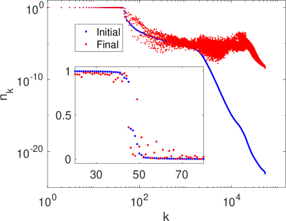
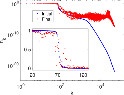
Figure 1: In the upper and lower panels we show the initial and final proton and neutron single-particle occupation probabilities, evaluated performing a fission simulation of ²³⁶U with the NEDF SeaLL1, starting near the top of the outer fission barrier, with the full set of initial quasi-particle wave functions, see Table 3, until the FFs are partially fully separated. Since the occupation probabilities are double degenerate, we display only 1/2 of their spectrum, in this case only $\Omega=54,000$. The results presented in this figure were obtained with $Q_{20}=140.02$ b and $Q_{30}=14.63$b^3/2 set of initial conditions.

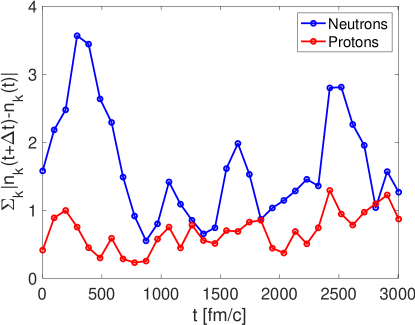
Figure 2: Total absolute difference between single-particle occupation probabilities at time $t$ and time $t+\Delta t$, where $\Delta t$ = 97 fm/c. Initial conditions are the same as in Fig. 1.

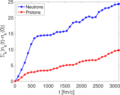
Figure 3: The sum of the absolute differences between the single-particle occupation probabilities at the initial time and at time $t$. Initial conditions are the same as in Fig. 1.

VI.2 Non-Markovian character of fission dynamics

In Fig. 1 we compare the initial canonical occupation probabilities $n_{k}(0)$ for both neutrons and protons, which change by more than 20 orders of magnitude, numbers we claim are numerically accurate, see also Ref. Bulgac et al. (2023), with the final occupation probabilities $n_{k}(t)=\sumint d\xi|{\text{v}}_{k}(\xi,t)|^{2}$, obtained from the time evolved ${\text{v}}_{k}$-components of the quasiparticle wave functions. As we mentioned above and in Refs. Bulgac et al. (2023); Bulgac (2022, 2023a, 2023b), even if one starts with a set of canonical wave functions, at the next time-step these wave functions fail to remain canonical. This is understandable, as in a framework where particle collisions are allowed, and they are allowed when pairing is taken into account beyond the static BCS approximation, the single-particle occupation probabilities change Bertsch (1980); Bertsch et al. (1987); Bertsch and Flocard (1991); Bertsch (1994); Bertsch and Bulgac (1997); Stetcu et al. (2011); Bulgac et al. (2019, 2020, 2023) and the canonical occupation probabilities change in time, which means the entropy of the system changes. See the discussion of Figs. 11-12 below.

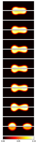
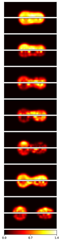
Figure 4: Time frames illustrating the profiles of the neutron (top) and proton number densities (first column) and the absolute value so the pairing gap (second column), separated in time by about 500 fm/c. The last row are for colorbars for the densities in units of fm^-3 and MeV for the pairing gaps. The initial state was the same as in Fig. 1.

In Figs. 2 and 3 we plot the sum of the absolute changes in the single-particle occupation probabilities $n_{k}(t)$ at some fixed time intervals $\Delta t=97$ fm/c and the absolute differences between the initial and time dependent single-particle occupation probabilities. Similar results have been reported in Ref. Bulgac (2022), however, with slightly different initial conditions for the same nucleus ²³⁶U with the same NEDF SeaLL1, but for smaller values of $\Delta t=37$ fm/c. In that case the initial quasiparticle wave functions were obtained using the code HFBTHO Navarro Perez et al. (2017), placed on the 3D spatial lattice, and only adjusting the proton and neutron chemical potentials to fix the correct average particle numbers. In all the simulations reported here we have run the static SLDA code on the 3D spatial lattice until full self-consistency was achieved. Since the phase space is much larger on a 3D spatial lattice than that used in HFBTHO code and since the kinetic energy and anomalous densities are formally diverging in a 3D space Bulgac (1980), the self-consistent SLDA equations need to be regularized and renormalized Bulgac and Yu (2002); Jin et al. (202). One important benefit of performing this additional self-consistency evaluation of the SLDA equations on the 3D spatial lattice is a much more numerically accurate solution of the TDSLDA equations.

These results demonstrate that during the entire fission dynamics, even after full the FF spatial separation, these occupation probabilities evolve with time, as expected for a non-equilibrium process of an isolated quantum system. These results provide a direct confirmation of the mechanism envisioned by Bertsch Bertsch (1980); Bertsch et al. (1987); Barranco et al. (1990, 1988); Bertsch and Bulgac (1997); Bulgac (2022), describing how nuclei experience shape changes through the redistribution of the single-particle occupation probabilities, facilitated by the pairing correlations and the correct implementation of the hydrodynamic continuity equation. The mechanism for nuclear shape change advocated by Bertsch implies that the single-particle occupation probabilities change through independent jumps at the single-particle level crossings and that these jumps are uncorrelated Bertsch (1980); Bertsch et al. (1987); Barranco et al. (1990, 1988); Bertsch and Bulgac (1997).

While the total particle number $\sum_{k}n_{k}(t)$ is conserved during the time evolution, the individual single-particle occupation probabilities change significantly, and one might be naively led to assume that the change of a particular occupation probability $0\leq n_{k}(t)\leq 1$ is random. If that would be the case, exactly as in the case of Brownian motion one would expect that

$$\sigma_{2}(t)=\sqrt{\sum_{k}(n_{k}(t)-n_{k}(0))^{2}}\propto\sqrt{t},$$ (99)

while the obviously, at large times, the closely related quantity $\sigma_{1}(t)$ illustrated in Fig. 3

$$\sigma_{1}(t)=\sum_{k}|n_{k}(t)-n_{k}(0)|\propto t,$$ (100)

which can be characterized as a “ballistic” behavior of the single-particle occupation probabilities $n_{k}(t)$, patently a non-stochastic and therefore non-Markovian behavior. Since we are solving quantum equations for quasiparticle wave functions the case can be made that instead of the quantity $\sigma_{1}(t)$ one should instead consider

$$\sigma_{0}(t)=\sum_{k}\left|\sqrt{n_{k}(t)}-\sqrt{n_{k}(0)}\right|,$$ (101)

since $\sqrt{n_{k}(t)}$ is proportional to the amplitude of each quasiparticle wave function ${\text{v}}_{k}(\xi,t)$, since these wave functions are the actual variables in the dynamic equations, similarly to the coordinates in the Langevin equation for example. The phases of the quasiparticle wave functions carry information about the currents, which to some extent were previously characterized by us when defining the collective flow kinetic energy Bulgac et al. (2019, 2020)

$$E_{coll}(t)=\int d{\bm{r}}\frac{mn({\bm{r}},t){\bm{v}}^{2}({\bm{r}},t)}{2},$$ (102)

where ${\bm{v}}({\bm{r}},t)$ is the hydrodynamic velocity of the nuclear matter. Unfortunately this quantity also includes after scission the accumulated FF kinetic energy due to their Coulomb repulsion, known as total kinetic energy of the FFs.

The quantum mechanical nature of the nuclear shape proves however to be more complex than envisioned by Bertsch Bertsch (1980); Bertsch et al. (1987); Barranco et al. (1990, 1988); Bertsch and Bulgac (1997); Bulgac (2022) and these jumps appear to be highly correlated in time, which is a qualitatively new aspect of fission dynamics in particular. This aspect is particularly interesting, since as we have proven in earlier fission simulations Bulgac et al. (2016b, 2019, 2020), the descent from the top of the outer barrier to the scission configuration is a highly dissipative process, in which case one would expect that stochasticity of the dynamics might play a crucial role. In the presence of a strong dissipation, stochasticity in case of classical dynamics and in numerous phenomenological fission models is modelled with a Langevin force Vogt et al. (2009); Vogt and Randrup (2013); Verbeke et al. (2018); Albertsson et al. ; Albertsson et al. (2020); Ishizuka et al. (2017); Randrup and Möller (2011); Randrup et al. (2011); Randrup and Möller (2013); Sierk (2017); Möller et al. (2001, 2004); Litaize et al. (2012); Becker et al. (2013). This is a qualitatively new situation in non-equilibrium dynamics, so far never discussed in literature as far as we can judge, where in the presence of strong dissipation, memory effects are also very strong and the single-particle occupation probabilities dynamics show a clear non-Markovian behavior.

The results in Figs. 2-3 show that the single-particle occupation probabilities, illustrated there at time intervals separated by $\Delta t=97$ fm/c change rather in a continuous manner and not as individual jumps. A jump at a “Landau-Zenner level crossing” is not instantaneous, but is coherently coupled with other jumps, which occur before or after a particular level crossing and that leads to a rather strong quantum coherence. In the end the change in the quantity $\sigma_{1}(t)$ instead of being random has a rather a well defined directed evolution, towards the equilibration of the quantum many-body system.

The quantity $\sigma_{1}(t)$ appears to change at two different rates for times smaller than 500-600 fm/c and at a slower rather for larger times. We see three different sources for this behavior. i) With time the strength of the pairing correlations and the absolute magnitude of the pairing gaps decreases, though it does never vanish, see Fig. 4 and  Bulgac et al. (2016b, 2019, 2020). ii) The fissioning nucleus and the FFs after separation still convert deformation energy into thermal energy, which leads to increasing occupation probabilities of higher energy single-particle states. iii) The neck appears to start forming at times 500-700 fm/c Bulgac et al. (2019); Bulgac (2022); Bulgac et al. (2023) and scission occurs at time 2,300-2,700 fm/c, depending on the initial conditions considered. In all TDDFT simulations one has to choose the initial nuclear shape but imposing a shape constraint and requiring that the total energy is near the outer fission barrier. The shape constraint is not inherent in the many-body Schrödinger equation and as in the initial Bohr and Wheeler (1939) paper this is merely a theoretical tool used since 1939. The nucleus during its descent from the top of the fission barrier needs to adjust to the absence of the artificial shape constraint imposed on the initial state. For times larger than 500-600 fm/c the nucleus appears to have settled to a different slower, but rather well defined rate, a bit higher for the neutron system than for the proton system. The neck, depending on its size, increasingly impedes matter, linear and angular momentum, and energy exchange between the two emerging FFs, and that is another reason why the rate of “equilibration” we see in Fig. 3 settles to a smaller value. At the same time, scission, which occurs at much later times, between 2,300-2,700 fm/c depending on the initial conditions and NEDF used, does not appear to affect this rate.

Ever since Boltzmann (1872) introduced the classical kinetic equations, and later on with their extension to quantum phenomena by Nordheim (1928) and Uehling and Uhlenbeck (1933), it was assumed that two-body collisions lead to a Markovian behavior of the many-body system, and thus to an absence of memory effects, similar to the case of Brownian motion of a single particle. The classical Boltzmann (1872) and the quantum extension of the collision integral due to Nordheim (1928) and Uehling and Uhlenbeck (1933) were stochastic in character. On the other hand, the extension of the TDDFT framework to superfluid phenomena is an extension of the time-dependent mean field dynamics to include a particular kind of collision term relevant in superfluids Bulgac (2022), as the action of the pairing field $\Delta(\xi,t)$ on the quasiparticle wave functions ${\text{u}}_{k}(\xi,t),{\text{v}}_{k}(\xi,t)$, see Eq. (65), which is not stochastic. The effect of this “quantum collision integral” is equivalent to the action of the collision term on the phase space occupation probabilities $f_{k}(q,p,t)$ in the Boltzmann-Nordheim (BN) Nordheim (1928) or Boltzmann-Uehling-Uhlenbeck (BUU) Uehling and Uhlenbeck (1933) kinetic equations. There is however a major difference: while in the “quantum” BN/BUU equations one operates with occupation probabilities, the TDSLDA equations Bulgac et al. (2011, 2012); Bulgac (2013, 2019, 2022) are formulated in terms of the quasiparticle wave functions, as expected in the case of a genuine quantum many-body framework. The consequences are quite fundamental, as TDSLDA can describe dynamical evolution of fermionic superfluids, in particular non-equilibrium dynamics; quantum turbulence; generation, life, dynamics, and decay of quantum vortices; entanglement; and nontrivial aspects of nuclear collisions Bulgac et al. (2011, 2016a); Magierski et al. (2017); Bulgac and Jin (2017); Pęcak et al. (2021); Magierski et al. (2022); Hossain et al. (2022), which are not accessible within a BN/BUU framework, since quantum interference and superpositions are not incorporated in the Boltzmann collision integral, either in its original classical form or that of Refs. Nordheim (1928); Uehling and Uhlenbeck (1933).

VI.3 Particle projection and use of a reduced set of canonical wave functions in time-dependent simulations

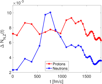
Figure 5: The standard deviation of the integrated proton and neutron particle projected densities $\Delta N_{Z,N}(t)$, defined in Eq. (103), as a functions of time. Somewhat surprisingly the differences between the integrated particle projected and unprojected number densities are very small, remembering that both $N$ and $Z$ are of ${\cal O}(100)$, thus the relative variance is at the level of ${\cal O}(10^{-4})$. The initial state was the same as in Table 1, but without the quadrupole collective energy boost.

We have estimated average discrepancies between the particle projected and unprojected number densities at various times

$$\Delta N_{N,Z}(t)=\sqrt{\sumint_{\xi}(n(\xi,\xi,t)-\tilde{n}(\xi,\xi,t|N))^{2}}.$$ (103)

and obtained a very similar relative trend, see Fig 5.

In Ref. Bulgac et al. (2023) we have established that the character of the canonical wave functions depends on the spatial resolution adopted in the numerical treatment, thus on the lattice constant $l$. The canonical wave functions with non-negligible occupation probabilities are localized in the region where the matter distribution of the system is non-vanishing and their number is typically much larger than the number of particles in the system, but significantly smaller than the size of the entire set, which is $2\Omega=2\times N_{x}N_{y}N_{z}$ for one type of nucleons. The spatial support for the canonical wave functions with negligible occupation probabilities is localized outside the region where matter distribution is localized. Obviously, the border between the two regions is not sharp. In this work we report more accurate estimates for the minimal number of canonical wave functions needed in order to obtain accurate enough numerical solutions in the case of heavy nuclei than in Ref. Bulgac et al. (2023).

In Fig. 6 we show the total energy ²³⁶U as a function of time, depending on various numbers of canonical wave functions used as an initial set. With the exception of the simulations with the entire set of quasi-particle wave functions and the entire set of canonical wave functions used as initial conditions, which are indistinguishable on this plot, every run performed with any number of wave functions as large as 50,000 initial canonical wave functions, failed to lead to fission, and moreover the total energy of the system is not conserved, the $Q_{20}$ of the entire system basically does not change in time. and the nucleus only keeps “heating up.” For any set of initial conditions, using the canonical wave functions with largest occupation probabilities in the interval $500,\ldots,50,000$, the nucleus does not fission, but only heats up. In the lower panel we display the behavior of the quadruple moment of the entire nucleus $Q_{20}(t)$ as a function of time for the same choice of initial conditions as for the upper panel. Only for the case when the entire set of quasi-particle or canonical wave functions is used the nucleus fissions, otherwise its size remains basically unchanged as a function of time. In this case the initial condition had an additional excitation energy of about 1.17 MeV and the simulations performed with a reduced set of canonical wave function still did not fission.

In Fig. 6, we report simulations performed with various limited sets of initial canonical quasi-particle wave functions. In past simulations, when we used a spherical cutoff for the pairing Bulgac and Yu (2002); Bulgac (2002); Bulgac et al. (2016b), which is extremely well suited for static calculations, we often observed that during time-evolution the system eventually failed numerically (overflow). Only after we gave up on using a spherical cutoff and implemented the entire spectrum Jin et al. (202) were we able to consistently obtain well behaved numerical solutions. It is remarkable to see that canonical states with an occupation number less that $10^{-10}$ acquire a significant occupation probability during the time-evolution. Furthermore, we have shown that the naive expectation that a reduced set of canonical quasi-particle wave functions, which reproduce nuclear properties of the initial state with very good accuracy, can be used to study the dynamics of fission, is incorrect.

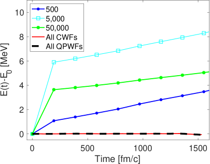
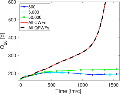
Figure 6: Plots of the time-dependence of the total energy of ²³⁶U, which theoretically should be conserved, as well as the time-dependence of the quadrupole moment, when various cutoffs are imposed on the initial set of canonical wave functions. The simulation with either the full set of quasi-particle or canonical wave functions are visually indistinguishable and in this case the total energy is conserved. These are results of simulation obtained with the set of initial deformation listed in Table 1.

The vast majority of simulations performed by other authors use the TDHF+BCS or TDHF+TDBCS approximation Zhang et al. (2023); Li et al. (2023a, b); Ren et al. (2022a, b); Bender and et al (2020); Scamps et al. (2015); Scamps and Simenel (2018); Scamps and Hashimoto (2019), where TD stands for time-dependent and HF for Hartree-Fock. Either the BCS or TDBCS approximations are further approximations to the TD Hartree-Fock-Bogoliubov (TDHFB) equations with cutoffs in the number of levels allowed to participate in pairing. Moreover, both BCS and TDBCS assume the spatial profiles of the $|{\text{u}}_{k}|^{2}$ and $|{\text{v}}_{k}|^{2}$-components of the quasi-particle wave functions are identical, as in the initial BCS approximation Bardeen et al. (1957) for weak pairing correlations. Even further, the continuity equation is violated in the TDHF+TDBCS approximation Scamps et al. (2012), which is still widely used today despite this Zhang et al. (2023); Li et al. (2023a, b); Ren et al. (2022a, b); Bender and et al (2020); Scamps et al. (2015); Scamps and Simenel (2018); Scamps and Hashimoto (2019) (to list a few studies).

Both BCS and TDBCS represent more limited approximations than evolving a truncated set of canonical quasi-particle wave functions, or using a spherical cutoff, as was originally done in Bulgac et al. (2016b). As described above, all trajectories performed in the canonical basis with a cutoff didn’t fission. This is likely the reason why BCS and TDBCS simulations of (induced) fission Zhang et al. (2023); Li et al. (2023a, b); Ren et al. (2022a, b); Bender and et al (2020); Scamps et al. (2015); Scamps and Simenel (2018); Scamps and Hashimoto (2019) start with initial compound nuclei on the potential energy surface of the fissioning nucleus that are well below the saddle point state of the nucleus considered. Only in such situations, for configurations where the Coulomb repulsion considerably exceeds the nuclear surface energy, could such simulations produce separated fission fragments.

As Meitner and Frisch (1939) correctly suggested, the nucleus during fission behaves like a liquid drop. Fission is due to the competition between the Coulomb and surface energies, and a correct hydrodynamic description of the nuclear shape dynamics is crucial, both at the classical and quantum level. How to achieve the correct description in the case of nuclei was not clear until Bertsch Bertsch (1980); Bertsch et al. (1987); Bertsch and Flocard (1991); Bertsch and Bulgac (1997) identified the crucial role played by the pairing dynamics in the shape evolution of a fissioning nucleus, which was confirmed in 2016 in the first correct implementation of pairing dynamics for this process Bulgac et al. (2016b).

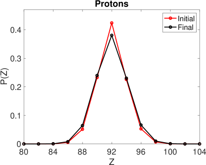
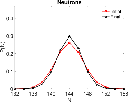
Figure 7: In the upper and lower panels we show the probabilities $P(N)$ defined in Eq. (79) for protons and neutrons respectively, in the initial and final states and used in producing Figs. 8-10, without any energy boost, as discussed in the text.

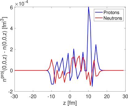
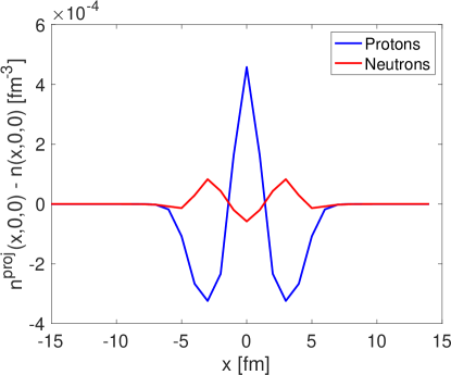
Figure 8: Differences between unprojected and particle projected number densities at the top of the outer barrier for ²³⁶U.

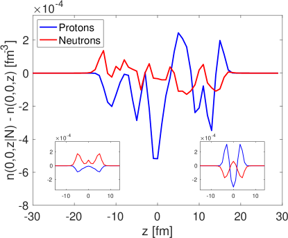
Figure 9: Differences between unprojected and particle projected number densities at the scission configuration, for the entire system along the fission direction $z$-axis and along the $x$-axis and at $y=0$ in the inserts, centered at the heavy on the left and at the light on the right fission fragments respectively at scission. In this case and in Figs. 8 and 10 the initial state was the same as in Table 1, but without a boost of the collective quadruple mode.

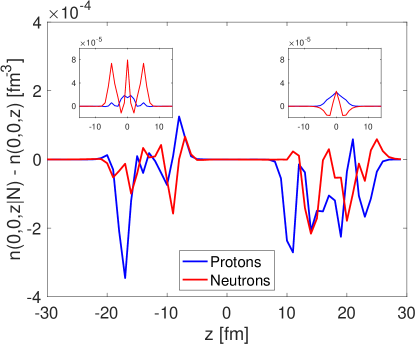
Figure 10: The same as in Fig. 9 but for the fully separated FFs.

The projected particle probability distributions $P(N)$, see Eq. (79), for protons and neutrons obtained are shown in Fig. 7, are slightly asymmetric with respect to the average proton $Z=92$ and neutron $N=144$ numbers. In Figs. 8-10 we show the differences between the unprojected and particle-projected number densities for protons and neutrons in the case of the induced fission of ²³⁶U at the top of the outer barrier, at the scission configurations, and for fully separated FFs. The densities were evaluated with 5,000 canonical quasi-particle wave functions, in which case the agreement at each time during the evolution with the entire set had very small relative errors, see also Fig 5.

VI.4 Irreversibility in isolated quantum systems

Another relevant aspect for the nuclear dynamics, which can be revealed with the help of canonical wave functions, is the irreversible time evolution of an isolated nuclear system, before it emits any nucleons or before it couples with the electromagnetic fields and emits photons or later on $\beta$-particles after coupling with the weak interactions. An isolated excited nucleus has a vanishing von Neumann or Shannon entropy, which naively would point to the absence of any irreversible time-evolution of such a system, which clearly is incorrect. At the classical level one can evaluate the Boltzmann entropy of an excited system, which would clearly characterize the irreversible time evolution of the system. The non-equilibrium evolution of isolated quantum systems can be characterized however with the help of the entanglement entropy Calabrese and Cardy (2005, 2006); Alba and Calabrese (2017). The entanglement entropy is non-vanishing even in the ground states of interacting systems Srednicki (1993). There is however no unique definition of the entanglement entropy, as it is well known Nordheim (1928); Uehling and Uhlenbeck (1933); Srednicki (1993); Klich (2006); Boguslawski and Tecmer (2014); Klich (2006); Amico et al. (2008); Horodecki et al. (2009); Haque et al. (2009); Eisert et al. (2010); Boguslawski and Tecmer (2014); Gigena and Rossignoli (2015); Bengtsson and Życzkowski (2017); Johnson (2018); Robin et al. (2021); Hoppe et al. (2021); Johnson and Gorton (2022); Bulgac (2022, 2023a, 2023b); Tichai et al. ; Fasano et al. (2022); Bulgac et al. (2023); Robin and Savage (2023); Gu et al. (2023); Pandharipande et al. (1984); Stoitsov et al. (1993); Reinhard et al. (1999); Dobaczewski et al. (1996); Tajima (2004); Tichai et al. (2019); Fasano et al. (2022); Chen et al. (2022); Hu et al. (2022); Hagen et al. (2022); Kortelainen et al. (2022). For nuclear systems, and particularly for heavy nuclei, which have an enormous number of degrees of freedom only the orbital entropy can be evaluated in the near future

$$S(t)= -g\sumint_{k}n_{k}(t)\ln n_{k}(t)$$

$$-g\sumint_{k}[1-n_{k}(t)]\ln[1-n_{k}(t)],$$ (104)

where $g$ is the spin-isospin degeneracy and the number of single-particle canonical occupation probabilities is of the order of ${\cal O}(10^{4\ldots 5})$, determined at each time shown with a symbol in Fig. 11. The entanglement entropy in addition provides an insight on the complexity, or the minimal number of independent Slater determinants, required to accurately describe a dynamic process as a function of time Bulgac et al. (2023). At different times during the evolution the complexity of the many-body wave function changes, depending on how effective is the repopulation of the single-particle states due to the particle-particle interactions, beyond the naive mean field. In a simple one Slater determinant time-dependent approximation, known as TDHF, the single particle occupation probabilities do not change in time.

Other authors have considered higher order entropies, such as two-body entropies Robin et al. (2021); Robin and Savage (2023); Gu et al. (2023), however, only in much smaller single-particle spaces than what is needed to simulate dynamics of complex nuclei, such as fission. The single-particle occupation probabilities are not well-defined, as their values depend of the basis set one uses in order to evaluate them, and a superfluid system is particular example. As it is well known for decades now, the canonical wave functions or the natural orbitals Löwdin and Shull (1956); Löwdin (1956); Coleman (1963a, b) are the smallest possible set to represent a many-body wave functions in terms of single-particle orbitals as a sum over $N$-particle Slater determinants, as in particular is needed in shell-model calculations Johnson (2018). For example, evaluating the entanglement two-body entropy Robin et al. (2021) would require defining the two-body density matrix

$$n_{2}(\xi,\zeta,\zeta^{\prime},\xi^{\prime})=\langle\Phi|\psi^{\dagger}(\xi^{\prime})\psi^{\dagger}(\zeta^{\prime})\psi(\zeta)\psi(\xi)|\Phi\rangle,$$ (105)

which in the case of nuclear systems simulated on a spatial lattice, is an object with $(2\times 2\times N_{x}N_{y}N_{z})^{4}$ coordinates, a quantity too large to fit in any classical supercomputers in the foreseeable future.

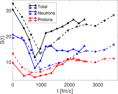
Figure 11: The orbital entropy $S(t)$ as a function for time for fission of ²³⁶U in a large simulation box $48^{2}\times 120$ fm³ for two of the simulations reported in Ref. Abdurrahman et al. (2023), for two different set of initial conditions. The initial deformations of the fissioning nuclei were $Q_{20}=159.64$ b and $Q_{30}=17.80$ b^3/2 for one trajectory (solid lines) and $Q_{20}=135.25$ b and $Q_{30}=12.44$ b^3/2 for the other trajectory (dashed lines), near the top of the outer barrier. The entropy is plotted separately for proton and neutron subsystems and for the entire fissioning system. For more details concerning these simulations see Ref. Abdurrahman et al. (2023).

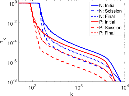
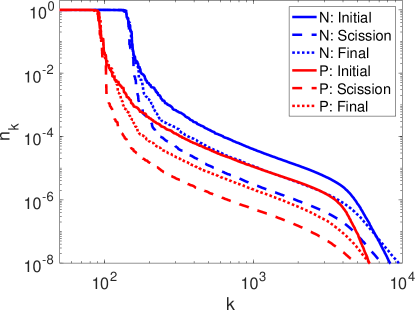
Figure 12: The time evolution of the canonical occupation probabilities for neutron and proton levels at the initial time, scission, and the final time, for the same data presented in Fig. 11. The upper panel correspond the trajectory shown with dashed limes, while the lower panel corresponds to the trajectory shown with solid lines in Fig. 11.

Here we will illustrate the irreversible fission dynamics in the largest simulation we have performed on a spatial lattice $48^{2}\times 120$, which required 4,609 nodes with 27,654 GPUs on the Summit supercomputer for about 15 wall-hours for a single fission trajectory, in one of the largest (if not the largest) direct numerical simulation ever reported, see Fig. 11. Similar results have been reported in Ref. Bulgac (2022, 2023a, 2023b); Bulgac et al. (2023) for both fission and for a ²³⁸U+²³⁸U collision at 1,500 MeV in center-of-mass frame, however for much smaller simulation boxes. The orbital entanglement entropy is very large initially, as expected in a system with very strong pairing correlations. As the nucleus evolves towards scission it heats up, achieving temperatures above 1 MeV Bulgac et al. (2016b, 2019, 2020) and the pairing correlations weaken, but they do not disappear, see Refs. Bulgac et al. (2016b, 2019, 2020) and Fig. 4. As Magierski et al. (2022) have recently shown, even in the high energy collisions of ⁹⁰Zr+⁹⁰Zr, due to the excitation of the Higgs pairing mode Barankov and Levitov (2006); Bulgac and Yoon (2009), pairing correlations, which are absent in the initial nuclei, acquire a large amplitude at very large excitation energies in the proximity of the Coulomb barrier of the colliding nuclei of the compound nucleus formed in this collision. While approaching the scission configuration, the matter exchange between the two halves of the fissioning nucleus slows down and completely stops after scission, which in the Fig. 11 is around 1,000 fm/c. After the two FFs separate, they are highly excited, and in particular the light FF is also very highly deformed, and both fragment relax, and the entanglement entropy increases with time, as the single-particle levels are repopulated, reaching values almost equal to the initial entanglement entropy of the cold strongly correlated nucleus near the top of the outer barrier. The temperature of the final FFs is significantly larger, the remaining pairing correlations are weaker, and while one process favors more occupation particle redistribution, the other works in the opposite direction.

In Fig. 3 and subsection VI.2 we observed the non-Markovian behavior of the quantity $\sigma_{1}(t)=\sum_{k}|n_{k}(t)-n_{k}(0)|$, which had a higher essentially linear rate of change before the neck is formed, and a slower, also almost linear rate for larger times. Between the initial state and scission the canonical occupation probability spectrum acquires a somewhat sharper Fermi surface, see Fig. 12, which explains why the orbital entropy decreases. In the final state the canonical occupation probability spectrum moves towards that of the initial state, which again explains why the orbital entanglement entropy increases. These two time-dependent behaviors of the $\sigma_{1}(t)$ and $S(t)$ are thus correlated and now we see how.

In the large simulation box we studied the fission of ²³⁶U we thus have clearly identified two regimes. In this very large simulation box the FFs still evolve in time when they reach the box walls and they clearly did not reach thermalization. One might be tempted to isolate each FF separately and follow its evolution in its own center-of-mass. This can appear physically motivated, as at sufficiently large spatial separations one expects that the FFs can hardly influence each other any longer, apart from the relatively weak Coulomb field. It is however not clear how one can formally proceed, since apart from the ${\text{v}}_{k}(\xi,t)$ quasiparticle wave functions, which can be very well localized inside a specific FF, the time evolution of a specific FF is also controlled by the ${\text{u}}_{k}(\xi,t)$ component of the quasiparticle wave functions, which are mostly fully delocalized, as we discussed in Section III, and through these components the two FFs can “communicate” with each other. This formal aspect of the TDDFT has not been developed yet.

This quantum non-equilibrium entanglement entropy Calabrese and Cardy (2005, 2006); Alba and Calabrese (2017) has an unexpected behavior at first sight, but this behavior is also observed in the evolution of other much simpler systems of strongly interacting fermions  Milburn et al. (1997); Chuchem et al. (2010); Cohen et al. (2016); Abanin et al. (2019); Sinha and Sinha (2020); Del Maestro et al. (2021, 2022); Thamm et al. (2022). As a final remark, even though we have illustrated the dynamics of a heavy nucleus with only a few examples, the same features were observed for several hundred fission trajectories and heavy-ion collisions we have performed over the years for various actinides and combination of heavy-ions, the latest still unpublished.

While we have not shown the occupation probability spectrum at scission, qualitatively it looks somewhat similar to the final occupation probability in the final state shown in Fig. 1. As we have discussed above, even if one starts a dynamical simulation with a set of canonical wave functions, they cease to be canonical at the next time step. The canonical occupation probability spectrum has to be determined separately at each time is needed, following the procedure outlined in Section II. In Fig. 12 we show canonical occupation probabilities, needed to evaluate the orbital entropy $S(t)$ at the initial, scission and final time. Unlike the final occupation probability spectrum shown in Fig. 1 the canonical occupation probability has a qualitatively similar character at any time. At scission however, both neutron and proton canonical occupation probabilities show noticeably shorter tails, which explains the non-monotonic behavior of the orbital entropy $S(t)$ illustrated in Fig. 11.

VII Conclusions

The use of a reduced set of canonical wave functions/natural orbitals could be a good approximation for treating a variety of static problems, when a reduced set of single-particle states with non-negligible occupation probabilities above a certain threshold are chosen. Unlike the normal number density, the anomalous number density and the kinetic energy density are strictly diverging in the case of local pairing potentials Bulgac (1980), since for large energies in 3D the single particle occupation probabilities behave as $n(\varepsilon(p))\propto 1/\varepsilon^{2}(p)\propto 1/p^{4}$, and regularization and renormalization are required in order to ensure accurate and reproducible results. The $1/p^{4}$ behavior of the canonical occupation probabilities is cutoff at momenta of the order of $\Lambda_{QCD}$ in nuclear systems or at $\hbar/r_{0}$, where $r_{0}$ is of the order of the range of the size of the particles. The canonical wave functions are also very useful when performing particle and/or angular momentum projections Scamps et al. (2023).

We have presented compelling arguments for the use of a full set of quasi-particle wave functions in time-dependent density functional theory simulations. The use of a smaller set of quasi-particle wave functions, or approximations such as TDBCS, lead to incorrect results or even fail to fission entirely. In a correct implementation of the dynamics, quasi-particle levels with even very small occupation probability, including those completely negligible at an initial time, quite often are populated at a later time to such a level that the final results could be qualitatively different between approximate and exact results. One should remember that the TDBCS approximation, which is a further approximation of the full TDHFB, is still using a reduced set of initial canonical quasi-particle wave functions, an approximation which leads to errors, as we have shown here. This approach quite widely used by a number of practitioners, which apart from violating the continuity equation, and thus failing to correctly describe the nuclear shape evolution, can lead to results quite different from the full TDDFT framework. In systems with strong pairing, such as nuclear systems and cold atom systems, the $u-$ and $v-$components of the Bogoliubov quasi-particle wave functions, where the $u$-component often lies in the continuum, or the exact time-reverse canonical orbitals $\phi_{k}(\xi)$ and $\phi_{\overline{k}}(\xi)$ have very different spatial profiles and cannot be treated in the BCS approximation.

We have demonstrated that using static self-consistent solutions of the DFT including pairing correlations with local pairing potentials lead different results, depending on whether one uses a BCS or a full HFB implementation of pairing correlations, the final solution depends quite strongly on the level of spatial resolution adopted, either by using a spatial lattice or a set of appropriately rescaled harmonic oscillator wave functions, as in the very popular code HFBTHO Navarro Perez et al. (2017); Marević et al. (2022). This is an important aspect of defining various nuclear energy density functionals, since because of the inherent divergence of the anomalous density Bulgac (1980), the self-consistent equations have to be regularized and renormalized Bulgac and Yu (2002); Bulgac (2002) in each specific numerical implementation, in total analogy with running coupling constants in quantum field theory, and it is not enough to specify the values of the coupling constants alone, but also the equivalent spatial resolution used in order to obtain nuclear masses, charge radii and other nuclear properties. This aspect becomes even more important in time-dependent simulations, since depending on the level of spatial resolution, the available phase space varies significantly and so does the dynamical evolution and the instantaneous single-particle occupation probabilities. Ignoring these aspects, particularly in simulation at relatively low spatial resolutions leads to vastly different properties of the final states, and thus the confrontation of the theory with experimental data becomes questionable.

Finally, we have shown how the use of time-dependent canonical occupation probabilities allows the determination of the orbital entanglement entropy, which provides insight into the irreversible dynamics of isolated quantum systems. This, in particular in the case of fission dynamics, also gives information about the time-dependence of the complexity of the many-body wave function of a strongly interacting system. The presence of pairing correlations within the TDDFT extension is tantamount to the presence of a quantum collision integral in the evolution equations Bulgac (2022), which leads to an obviously non-Markovian behavior, unexpected in the presence of strong dissipation in a traditional Nordheim (1928) and Uehling and Uhlenbeck (1933) formulation of the quantum kinetic theory. The extension of the TDDFT framework to superfluid systems has similarities with the Baym and Kadanoff extension framework Baym and Kadanoff (1961, 1962), see also the independent work of Keldysh (1965). These extensions of the non-equilibrium dynamics are however much more complex as they rely on very complex memory and non-local kernels, and their application to such a complex phenomenon as nuclear fission, would be numerically impossible in the foreseeable future. Unlike the von Neumann or Shannon entropy, which vanishes for an isolated quantum system and thus fails to describe the irreversible dynamics and the expected thermalization of the excited nuclei, the orbital entanglement entropy is likely the most useful characterization of the quantum dynamics of an isolated nucleus, which can be evaluated for rather complex time-dependent many-body systems.

Acknowledgements

We have benefited at various times from discussions on issues discussed here with K. Godbey, G. Scamps, and A. Makowski. The funding for AB from the Office of Science, Grant No. DE-FG02-97ER41014 and also the partial support provided by NNSA cooperative Agreement DE-NA0003841 is greatly appreciated. MK was supported by NNSA cooperative Agreement DE-NA0003841. This work was carried out under the auspices of the National Nuclear Security Administration of the U.S. Department of Energy at Los Alamos National Laboratory under Contract No. 89233218CNA000001, and used resources of the Oak Ridge Leadership Computing Facility, which is a U.S. DOE Office of Science User Facility supported under Contract No. DE-AC05-00OR22725. I.A. and I.S. gratefully acknowledges partial support and computational resources provided by the Advanced Simulation and Computing (ASC) Program.

References

- Bardeen et al. (1957) J. Bardeen, L. N. Cooper, and J. R. Schrieffer, “Theory of superconductivity,” Phys. Rev. 108, 1175 (1957).
- Löwdin (1956) P.-O. Löwdin, “Quantum theory of cohesive properties of solids,” Adv. Phys. 5, 1 (1956).
- Löwdin and Shull (1956) P.-O. Löwdin and H. Shull, “Natural orbitals in the quantum theory of two-electron systems,” Phys. Rev. 101, 1730–1739 (1956).
- Coleman (1963a) A. J. Coleman, “Structure of fermion density matrices,” Rev. Mod. Phys. 35, 668 (1963a).
- Coleman (1963b) A. J. Coleman, “Discussion on "structure of fermion density matrices",” Rev. Mod. Phys. 35, 687 (1963b).
- Davidson (1972) E. R. Davidson, “Properties and Uses of Natural Orbitals,” Rev. Mod. Phys. 44, 451 (1972).
- Bogoliubov (1958) N. N. Bogoliubov, “On a new method in the theory of superconductivity,” Il Nuovo Cimento 7, 794 (1958).
- Valatin (1958) J. G. Valatin, “Comments on the theory of superconductivity,” Il Nuovo Cimento 7, 843 (1958).
- Bulgac (1980) A. Bulgac, “Hartree-Fock-Bogoliubov approximation for finite systems,” (1980), arXiv:nucl-th/9907088 .
- Bulgac et al. (2023) A. Bulgac, M. Kafker, and I. Abdurrahman, “Measures of complexity and entanglement in many-fermion systems,” Phys. Rev. C 107, 044318 (2023).
- Chen et al. (2022) M. Chen, T. Li, B. Schuetrumpf, P.-G. Reinhard, and W. Nazarewicz, “Three-dimensional Skyrme Hartree-Fock-Bogoliubov solver in coordinate-space representation,” Comp. Phys. Comm. 276, 108344 (2022).
- Ring and Schuck (2004) P. Ring and P. Schuck, The Nuclear Many-Body Problem, 1st ed. (Springer-Verlag, Berlin Heidelberg New York, 2004).
- Bloch and Messiah (1962) C. Bloch and A. Messiah, “The canonical form of an antisymmetric tensor and its application to the theory of superconductivity,” Nucl. Phys. 39, 95 (1962).
- Zumino (1962) B. Zumino, “Normal Forms of Complex Matrices,” J. Math. Phys. 3, 1055 (1962).
- Bulgac (2021) A. Bulgac, “Restoring broken symmetries for nuclei and reaction fragments,” Phys. Rev. C 104, 054601 (2021).
- Robledo (2009) L. M. Robledo, “Sign of the overlap of Hartree-Fock-Bogoliubov wave functions,” Phys. Rev. C 79, 021302 (2009).
- Bertsch and Robledo (2012) G. F. Bertsch and L. M. Robledo, “Symmetry Restoration in Hartree-Fock-Bogoliubov Based Theories,” Phys. Rev. Lett. 108, 042505 (2012).
- Carlsson and Rotureau (2021) B. G. Carlsson and J. Rotureau, “New and Practical Formulation for Overlaps of Bogoliubov Vacua,” Phys. Rev. Lett. 126, 172501 (2021).
- Magierski et al. (2017) P. Magierski, K. Sekizawa, and G. Wlazłowski, “Novel role of superfluidity in low-energy nuclear reactions,” Phys. Rev. Lett. 119, 042501 (2017).
- Magierski et al. (2022) P. Magierski, A. Makowski, M. C. Barton, K. Sekizawa, and G. Wlazłowski, “Pairing dynamics and solitonic excitations in collisions of medium-mass, identical nuclei,” Phys. Rev. C 105, 064602 (2022).
- Bulgac and Jin (2017) A. Bulgac and S. Jin, “Dynamics of Fragmented Condensates and Macroscopic Entanglement,” Phys. Rev. Lett. 119, 052501 (2017).
- Born (1926a) M. Born, “Quantenmechanik der Stoßvorgänge,” Zeitschrift für Physik 38, 803–827 (1926a).
- Born (1926b) M. Born, “Zur Quantenmechanik der Stoßvorgänge,” Zeitschrift für Physik 37, 863 (1926b).
- Heilbron and Rovelli (2023) J.L. Heilbron and C. Rovelli, “Matrix mechanics mis-prized: Max Born’s belated nobelization,” Eur. Phys. J. H 48, 11 (2023).
- (25) P. W. Anderson, in The Lesson of Quantum Theory, edited by J. de Boer, E. Dal, and O. Ulfbeck (North Holland, Elsevier, Amsterdam, 1986) pp. 23–34.
- Bulgac et al. (2019) A. Bulgac, S. Jin, K. J. Roche, N. Schunck, and I. Stetcu, “Fission dynamics of from saddle to scission and beyond,” Phys. Rev. C 100, 034615 (2019).
- Bulgac et al. (2020) A. Bulgac, S. Jin, and I. Stetcu, “Nuclear Fission Dynamics: Past, Present, Needs, and Future,” Frontiers in Physics 8, 63 (2020).
- Jin et al. (202) S. Jin, K. J. Roche, I. Stetcu, I.Abdurrahman, and A. Bulgac, “The LISE package: solvers for static and time-dependent superfluid local density approximation equations in three dimentions,” Comp. Phys. Comm. 269, 108130 (202).
- Bulgac and Yu (2002) A. Bulgac and Y. Yu, “Renormalization of the Hartree-Fock-Bogoliubov Equations in the Case of a Zero Range Pairing Interaction,” Phys. Rev. Lett. 88, 042504 (2002).
- Bulgac (2002) A. Bulgac, “Local density approximation for systems with pairing correlations,” Phys. Rev. C 65, 051305 (2002).
- Bulgac (2007) A. Bulgac, “Local-density-functional theory for superfluid fermionic systems: The unitary Fermi gas,” Phys. Rev. A 76, 040502 (2007).
- Tan (2008a) S. Tan, “Energetics of a strongly correlated Fermi gas,” Ann. Phys. 323, 2952 (2008a).
- Tan (2008b) S. Tan, “Large momentum part of a strongly correlated Fermi gas,” Ann. Phys. 323, 2971 (2008b).
- Tan (2008c) S. Tan, “Generalized virial theorem and pressure relation for a strongly correlated Fermi gas,” Ann. Phys. 323, 2987 (2008c).
- Bulgac et al. (2011) A. Bulgac, Y.-L. Luo, P. Magierski, K. J. Roche, and Y. Yu, “Real-Time Dynamics of Quantized Vortices in a Unitary Fermi Superfluid,” Science 332, 1288 (2011).
- Bulgac et al. (2012) A. Bulgac, M. M. Forbes, and P. Magierski, “The unitary Fermi gas: From Monte Carlo to density functionals,” Chap. 9, pp. 127 – 191, vol. 836 of Zwerger (2012) (2012).
- Zwerger (2012) W. Zwerger, ed., The BCS–BEC Crossover and the Unitary Fermi Gas, Lecture Notes in Physics, Vol. 836 (Springer-Verlag, Berlin Heidelberg, 2012).
- Braaten (2012) E. Braaten, “Universal Relations for Fermions with Large Scattering Length,” (Springer, Berlin Heidelberg, 2012) Chap. 6, pp. 193–231.
- Castin and Werner (2012) Y. Castin and F. Werner, “The Unitary Gas and its Symmetry Properties,” (Springer, Berlin Heodelberg, 2012) Chap. 5.
- Bulgac (2013) A. Bulgac, “Time-Dependent Density Functional Theory and the Real-Time Dynamics of Fermi Superfluids,” Ann. Rev. Nucl. and Part. Sci. 63, 97 (2013).
- Bulgac et al. (2016a) A. Bulgac, M. M. Forbes, and W. Wlazłowski, “Towards quantum turbulence in cold atomic fermionic superfluids,” J. Phys. B: At. Mol. Opt. Phys. 50, 014001 (2016a).
- Bulgac (2019) A. Bulgac, “Time-Dependent Density Functional Theory for Fermionic Superfluids: from Cold Atomic gases, to Nuclei and Neutron Star Crust,” Physica Status Solidi B 256, 1800592 (2019).
- Levinger (1951) J. S. Levinger, “The High Energy Nuclear Photoeffect,” Phys. Rev. 84, 43 (1951).
- Levinger (1979) J.S. Levinger, “Modified quasi-deutron model,” Physics Letters B 82, 181–182 (1979).
- Levinger (2002) J.S. Levinger, “Fifty years of the quasi-deuteron model,” Nuclear Physics A 699, 255–260 (2002), 3rd Int. Conf. on Perspectives in Hadronic Physics.
- Tropiano et al. (2022) A. J. Tropiano, S. K. Bogner, R. J. Furnstahl, and M. A. Hisham, “Quasi-deuteron model at low renormalization group resolution,” Phys. Rev. C 106, 024324 (2022).
- Tropiano et al. (2021) A. J. Tropiano, S. K. Bogner, and R. J. Furnstahl, “Short-range correlation physics at low renormalization group resolution,” Phys. Rev. C 104, 034311 (2021).
- O. Hen et al. (2014) O. Hen et al., “Momentum sharing in imbalanced Fermi systems,” Science 346, 614 (2014).
- Hen et al. (2017) O. Hen, G. A. Miller, E. Piasetzky, and L. B. Weinstein, “Nucleon-nucleon correlations, short-lived excitations, and the quarks within,” Rev. Mod. Phys. 89, 045002 (2017).
- Cruz-Torres et al. (2018) R. Cruz-Torres, A. Schmidt, G.A. Miller, L.B. Weinstein, N. Barnea, R. Weiss, E. Piasetzky, and O. Hen, “Short range correlations and the isospin dependence of nuclear correlation functions,” Physics Letters B 785, 304 (2018).
- Cruz-Torres et al. (2021) R. Cruz-Torres, D. Lonardoni, R. Weiss, M. Piarulli, N. Barnea, D. W. Higinbotham, E. Piasetzky, A. Schmidt, L. B. Weinstein, R. B. Wiringa, and O. Hen, “Many-body factorization and position–momentum equivalence of nuclear short-range correlations,” Nature Physics 17, 306 (2021).
- Frankfurt and Strikman (1981) L.L. Frankfurt and M.I. Strikman, “High-energy phenomena, short-range nuclear structure and QCD,” Phys. Rep. 76, 215 (1981).
- Frankfurt and Strikman (1988) L. Frankfurt and M. Strikman, “Hard nuclear processes and microscopic nuclear structure,” Phys. Rep. 160, 235 (1988).
- Piasetzky et al. (2006) E. Piasetzky, M. Sargsian, L. Frankfurt, M. Strikman, and J. W. Watson, “Evidence for Strong Dominance of Proton-Neutron Correlations in Nuclei,” Phys. Rev. Lett. 97, 162504 (2006).
- Sargsian et al. (2005) M. M. Sargsian, T. V. Abrahamyan, M. I. Strikman, and L. L. Frankfurt, “Exclusive electrodisintegration of at high . ii. decay function formalism,” Phys. Rev. C 71, 044615 (2005).
- Carlson et al. (2015) J. Carlson, S. Gandolfi, F. Pederiva, Steven C. Pieper, R. Schiavilla, K. E. Schmidt, and R. B. Wiringa, “Quantum monte carlo methods for nuclear physics,” Rev. Mod. Phys. 87, 1067–1118 (2015).
- Schiavilla et al. (2007) R. Schiavilla, R. B. Wiringa, S. C. Pieper, and J. Carlson, “Tensor forces and the ground-state structure of nuclei,” Phys. Rev. Lett. 98, 132501 (2007).
- Bulgac (2022) A. Bulgac, “Pure quantum extension of the semiclassical Boltzmann-Uehling-Uhlenbeck equation,” Phys. Rev. C 105, L021601 (2022).
- Bulgac (2023a) A. Bulgac, “Entropy, single-particle occupation probabilities, and short-range correlations,” Phys. Rev. C 107, L061602 (2023a).
- Bulgac (2023b) A. Bulgac, “New developments in fission studies within the time-dependent density functional theory framework,” EPJ Web of Conferences 284, 04001 (2023b).
- Stringari and Brink (1978) S. Stringari and D.M. Brink, “Constraints on effective interactions imposed by antisymmetry and charge independence,” Nuclear Physics A 304, 307 (1978).
- Perdew and Zunger (1981) J. P. Perdew and Alex Zunger, “Self-interaction correction to density-functional approximations for many-electron systems,” Phys. Rev. B 23, 5048 (1981).
- Stoitsov et al. (2007) M. V. Stoitsov, J. Dobaczewski, R. Kirchner, W. Nazarewicz, and J. Terasaki, “Variation after particle-number projection for the Hartree-Fock-Bogoliubov method with the Skyrme energy density functional,” Phys. Rev. C 76, 014308 (2007).
- Bender et al. (2003) M. Bender, P.-H. Heenen, and P.-G. Reinhard, “Self-consistent mean-field models for nuclear structure,” Rev. Mod. Phys. 75, 121 (2003).
- Dobaczewski et al. (2007) J. Dobaczewski, M. V. Stoitsov, W. Nazarewicz, and P.-G. Reinhard, “Particle-number projection and the density functional theory,” Phys. Rev. C 76, 054315 (2007).
- Duguet et al. (2009) T. Duguet, M. Bender, K. Bennaceur, D. Lacroix, and T. Lesinski, “Particle-number restoration within the energy density functional formalism: Nonviability of terms depending on noninteger powers of the density matrices,” Phys. Rev. C 79, 044320 (2009).
- Bender et al. (2009) M. Bender, T. Duguet, and D. Lacroix, “Particle-number restoration within the energy density functional formalism,” Phys. Rev. C 79, 044319 (2009).
- Lacroix et al. (2009) D. Lacroix, T. Duguet, and M. Bender, “Configuration mixing within the energy density functional formalism: Removing spurious contributions from nondiagonal energy kernels,” Phys. Rev. C 79, 044318 (2009).
- Hupin et al. (2011) G. Hupin, D. Lacroix, and M. Bender, “Formulation of functional theory for pairing with particle number restoration,” Phys. Rev. C 84, 014309 (2011).
- Duguet et al. (2015) T. Duguet, M. Bender, J. P. Ebran, T. Lesinski, and V. Somà, “Ab initio-driven nuclear energy density functional method,” The Eur. Phys. J. A 51, 162 (2015).
- Sheikh et al. (2021) J. A. Sheikh, J. Dobaczewski, P. Ring, L. M .Robledo, and C. Yannouleas, “Symmetry restoration in mean-field approaches,” Journal of Physics G: Nuclear and Particle Physics 48, 123001 (2021).
- Kohn and Sham (1965) W. Kohn and L. J. Sham, “Self-Consistent Equations Including Exchange and Correlation Effects,” Phys. Rev. 140, A1133 (1965).
- Bulgac and Forbes (2013) A. Bulgac and M. M. Forbes, “Use of the discrete variable representation basis in nuclear physics,” Phys. Rev. C 87, 051301(R) (2013).
- Bulgac et al. (2018) A. Bulgac, M. M. Forbes, S. Jin, R. Navarro Perez, and N. Schunck, “Minimal nuclear energy density functional,” Phys. Rev. C 97, 044313 (2018).
- Navarro Perez et al. (2017) R. Navarro Perez, N. Schunck, R.-D. Lasseri, C. Zhang, and J. Sarich, “Axially deformed solution of the Skyrme–Hartree–Fock–Bogolyubov equations using the transformed harmonic oscillator basis (III) HFBHTO (v3.00): A new version of the program,” Comp. Phys. Comm. 220, 363 (2017).
- Bertsch (1980) G. Bertsch, “The nuclear density of states in the space of nuclear shapes,” Phys. Lett. B 95, 157 (1980).
- Bertsch et al. (1987) G. F. Bertsch, F. Barranco, and R. A. Broglia, in Windsurfing the Fermi Sea: Proceedings of the International Conference and Symposium on Unified Concepts of Many-Body Problems, edited by T. T. S. Kuo and J. Speth (North-Holland, Amsterdam, 1987) p. 33.
- Bertsch and Flocard (1991) G. Bertsch and H. Flocard, “Pairing effects in nuclear collective motion: Generator coordinate method,” Phys. Rev. C 43, 2200 (1991).
- Bertsch (1994) G.F. Bertsch, “Large amplitude collective motion,” Nuclear Physics A 574, 169 – 183 (1994).
- Bertsch and Bulgac (1997) G. F. Bertsch and A. Bulgac, “Comment on “spontaneous fission: A kinetic approach”,” Phys. Rev. Lett. 79, 3539 (1997).
- Stetcu et al. (2011) I. Stetcu, A. Bulgac, P. Magierski, and K. J. Roche, “Isovector giant dipole resonance from the 3D time-dependent density functional theory for superfluid nuclei,” Phys. Rev. C 84, 051309 (2011).
- Barranco et al. (1990) F. Barranco, G.F. Bertsch, R.A. Broglia, and E. Vigezzi, “Large-amplitude motion in superfluid Fermi droplets,” Nucl. Data Sheets Phys. A 512, 253 (1990).
- Barranco et al. (1988) F. Barranco, R. A. Broglia, and G. F. Bertsch, “Exotic radioactivity as a superfluid tunneling phenomenon,” Phys. Rev. Lett. 60, 50 (1988).
- Bulgac et al. (2016b) A. Bulgac, P. Magierski, K. J. Roche, and I. Stetcu, “Induced Fission of within a Real-Time Microscopic Framework,” Phys. Rev. Lett. 116, 122504 (2016b).
- Vogt et al. (2009) R. Vogt, J. Randrup, J. Pruet, and W. Younes, “Event-by-event study of prompt neutrons from ,” Phys. Rev. C 80, 044611 (2009).
- Vogt and Randrup (2013) R. Vogt and J. Randrup, “Event-by-event Modeling of Prompt Neutrons and Photons from Neutron-induced and Spontaneous Fission with FREYA,” Physics Procedia 47, 82 (2013), scientific Workshop on Nuclear Fission Dynamics and the Emission of Prompt Neutrons and Gamma Rays, Biarritz, France, 28-30 November 2012.
- Verbeke et al. (2018) J. M. Verbeke, J. Randrup, and R. Vogt, “Fission Reaction Event Yield Algorithm FREYA 2.0.2,” Comp. Phys. Com. 222, 263 (2018).
- (88) M. Albertsson, B.G. Carlsson, T. Døssing, P. Møller, J. Randrup, and S. Åberg, “Microscopic treatment of energy partition in fission,” arXiv:1811.02283 .
- Albertsson et al. (2020) M. Albertsson, B.G. Carlsson, T. Døssing, P. Möller, J. Randrup, and S. Åberg, “Excitation energy partition in fission,” Phys. Lett. B 803, 135276 (2020).
- Ishizuka et al. (2017) C. Ishizuka, M. D. Usang, F. A. Ivanyuk, J. A. Maruhn, K. Nishio, and S. Chiba, “Four-dimensional Langevin approach to low-energy nuclear fission of ,” Phys. Rev. C 96, 064616 (2017).
- Randrup and Möller (2011) J. Randrup and P. Möller, “Brownian Shape Motion on Five-Dimensional Potential-Energy Surfaces:Nuclear Fission-Fragment Mass Distributions,” Phys. Rev. Lett. 106, 132503 (2011).
- Randrup et al. (2011) J. Randrup, P. Möller, and A. J. Sierk, “Fission-fragment mass distributions from strongly damped shape evolution,” Phys. Rev. C 84, 034613 (2011).
- Randrup and Möller (2013) J. Randrup and P. Möller, “Energy dependence of fission-fragment mass distributions from strongly damped shape evolution,” Phys. Rev. C 88, 064606 (2013).
- Sierk (2017) A. J. Sierk, “Langevin model of low-energy fission,” Phys. Rev. C 96, 034603 (2017).
- Möller et al. (2001) P. Möller, D. G. Madland, A. J. Sierk, and A. Iwamoto, “Nuclear fission modes and fragment mass asymmetries in a five-dimensional deformation space,” Nature 409, 785 (2001).
- Möller et al. (2004) Peter Möller, Arnold J. Sierk, and Akira Iwamoto, “Five-dimensional fission-barrier calculations from to ,” Phys. Rev. Lett. 92, 072501 (2004).
- Litaize et al. (2012) Olivier Litaize, Olivier Serot, David Regnier, StŽphane Theveny, and SŽbastien Onde, “New Features of the FIFRELIN Code for the Investigation of Fission Fragments Characteristics,” Physics Procedia 31, 51 (2012), gAMMA-1 Emission of Prompt Gamma-Rays in Fission and Related Topics.
- Becker et al. (2013) B. Becker, P. Talou, T. Kawano, Y. Danon, and I. Stetcu, “Monte Carlo Hauser-Feshbach predictions of prompt fission rays: Application to U, Pu, and 252Cf (sf),” Phys. Rev. C 87, 014617 (2013).
- Bohr and Wheeler (1939) N. Bohr and J. A. Wheeler, “The Mechanism of Nuclear Fission,” Phys. Rev. 56, 426–450 (1939).
- Boltzmann (1872) L. Boltzmann, “Weitere Studien über das Wärmegleichgewicht unter Gasmolekülen,” Sitzungsberichte Akademie der Wissenschaften 66, 275 (1872).
- Nordheim (1928) L. W. Nordheim, “On the Kinetic Method in the New Statistics and its Application in the Electron Theory of Conductivity,” Proc. Roy. Soc. (London) A119, 689 (1928).
- Uehling and Uhlenbeck (1933) E. A. Uehling and G. E. Uhlenbeck, “Transport Phenomena in Einstein-Bose and Fermi-Dirac Gases. I,” Phys. Rev. 43, 552 (1933).
- Pęcak et al. (2021) Daniel Pęcak, Nicolas Chamel, Piotr Magierski, and Gabriel Wlazłowski, “Properties of a quantum vortex in neutron matter at finite temperatures,” Phys. Rev. C 104, 055801 (2021).
- Hossain et al. (2022) K. Hossain, K. Kobuszewski, M. M. Forbes, P. Magierski, K. Sekizawa, and G. Wlazłowski, “Rotating quantum turbulence in the unitary Fermi gas,” Phys. Rev. A 105, 013304 (2022).
- Zhang et al. (2023) D. D. Zhang, B. Li, D. Vretenar, T. Nikšić, Z. X. Ren, P. W. Zhao, and J. Meng, “Ternary quasifission in collisions of actinide nuclei,” (2023), arXiv:2310.02657 [nucl-th] .
- Li et al. (2023a) B. Li, D. Vretenar, T. Nikšić, J. Zhao, P. W. Zhao, and J. Meng, “Generalized time-dependent generator coordinate method for small and large amplitude collective motion (ii): pairing correlations and fission,” (2023a), arXiv:2309.12564 [nucl-th] .
- Li et al. (2023b) B. Li, D. Vretenar, Z. X. Ren, T. Nikšić, J. Zhao, P. W. Zhao, and J. Meng, “Fission dynamics, dissipation, and clustering at finite temperature,” Phys. Rev. C 107, 014303 (2023b).
- Ren et al. (2022a) Z. X. Ren, J. Zhao, D. Vretenar, T. Nikšić, P. W. Zhao, and J. Meng, “Microscopic analysis of induced nuclear fission dynamics,” Phys. Rev. C 105, 044313 (2022a).
- Ren et al. (2022b) Z. X. Ren, D. Vretenar, T. Nikšić, P. W. Zhao, J. Zhao, and J. Meng, “Dynamical Synthesis of in the Scission Phase of Nuclear Fission,” Phys. Rev. Lett. 128, 172501 (2022b).
- Bender and et al (2020) M. Bender and et al, “Future of nuclear fission theory,” J. Phys. G: Nucl. Part. Phys. 47, 113002 (2020).
- Scamps et al. (2015) G. Scamps, C. Simenel, and D. Lacroix, “Superfluid dynamics of fission,” Phys. Rev. C 92, 011602 (2015).
- Scamps and Simenel (2018) G. Scamps and C. Simenel, “Impact of pear-shaped fission fragments on mass-asymmetric fission in actinides,” Nature 564, 382–385 (2018).
- Scamps and Hashimoto (2019) G. Scamps and Y. Hashimoto, “Density-constrained time-dependent Hartree-Fock-Bogoliubov method,” Phys. Rev. C 100, 024623 (2019).
- Scamps et al. (2012) G. Scamps, D. Lacroix, G. F. Bertsch, and K. Washiyama, “Pairing dynamics in particle transport,” Phys. Rev. C 85, 034328 (2012).
- Meitner and Frisch (1939) L. Meitner, L. and O. R. Frisch, “Disintegration of Uranium by Neutrons: a New Type of Nuclear Reaction,” Nature 143, 239 (1939).
- Calabrese and Cardy (2005) P. Calabrese and J. Cardy, “Evolution of entanglement entropy in one-dimensional systems,” J. Stat. Mech 2005, P04010 (2005).
- Calabrese and Cardy (2006) P. Calabrese and J. Cardy, “Time Dependence of Correlation Functions Following a Quantum Quench,” Phys. Rev. Lett. 96, 136801 (2006).
- Alba and Calabrese (2017) V. Alba and P. Calabrese, “Entanglement and thermodynamics after a quantum quench in integrable systems,” Proc. Natl. Acad. Sci. USA 114, 7947 (2017).
- Srednicki (1993) M. Srednicki, “Entropy and area,” Phys. Rev. Lett. 71, 666 (1993).
- Klich (2006) I. Klich, “Lower entropy bounds and particle number fluctuations in a Fermi sea,” Journal of Physics A: Mathematical and General 39, L85 (2006).
- Boguslawski and Tecmer (2014) K. Boguslawski and P. Tecmer, “Orbital entanglement in quantum chemistry,” Int. J. Quant. Chem. 115, 1289 (2014).
- Amico et al. (2008) L. Amico, R. Fazio, A. Osterloh, and V. Vedral, “Entanglement in many-body systems,” Rev. Mod. Phys. 80, 517 (2008).
- Horodecki et al. (2009) R. Horodecki, P. Horodecki, M. Horodecki, and K. Horodecki, “Quantum entanglement,” Rev. Mod. Phys. 81, 865–942 (2009).
- Haque et al. (2009) M. Haque, O. S. Zozulya, and K. Schouten, “Entanglement between particle partitions in itinerant many-particle states,” J. Phys. A Math. Theor. 42, 504012 (2009).
- Eisert et al. (2010) J. Eisert, M. Cramer, and M. B. Plenio, “Colloquium: Area laws for the entanglement entropy,” Rev. Mod. Phys. 82, 277–306 (2010).
- Gigena and Rossignoli (2015) N. Gigena and R. Rossignoli, “Entanglement in fermion systems,” Phys. Rev. A 92, 042326 (2015).
- Bengtsson and Życzkowski (2017) I. Bengtsson and K. Życzkowski, GEOMETRY OF QUANTUM STATES (An Introduction to quantum entanglement), 2nd ed. (Cambridge University Press, 2017).
- Johnson (2018) C. W. Johnson, “Current Status of Very-Large-Basis Hamiltonian Diagonalizations for Nuclear Physics,” (2018), arXiv:1809.07869 .
- Robin et al. (2021) C. Robin, M. J. Savage, and N. Pillet, “Entanglement rearrangement in self-consistent nuclear structure calculations,” Phys. Rev. C 103, 034325 (2021).
- Hoppe et al. (2021) J. Hoppe, A. Tichai, M. Heinz, K. Hebeler, and A. Schwenk, “Natural orbitals for many-body expansion methods,” Phys. Rev. C 103, 014321 (2021).
- Johnson and Gorton (2022) C. W. Johnson and O. C. Gorton, “Proton-neutron entanglement in the nuclear shell model,” (2022), arXiv:2210.14338 .
- (132) A. Tichai, S. Knecht, A. T. Kruppa, Ö. Legeza, C. P. Moca, A. Schwenk, M. A. Werner, and G. Zarand, “Combining the in-medium similarity renormalization group with the density matrix renormalization group: Shell structure and information entropy,” arXiv:2207.01438 .
- Fasano et al. (2022) P. J. Fasano, C. Constantinou, M. A. Caprio, P. Maris, and J. P. Vary, “Natural orbitals for the ab initio no-core configuration interaction approach,” Phys. Rev. C 105, 054301 (2022).
- Robin and Savage (2023) C. E. P. Robin and M. J. Savage, “Quantum simulations in effective model spaces: Hamiltonian-learning variational quantum eigensolver using digital quantum computers and application to the Lipkin-Meshkov-Glick model,” Phys. Rev. C 108, 024313 (2023).
- Gu et al. (2023) C. Gu, Z. H. Sun, G. Hagen, and T. Papenbrock, “Entanglement entropy of nuclear systems,” Phys. Rev. C 108, 054309 (2023).
- Pandharipande et al. (1984) V. R. Pandharipande, C. N. Papanicolas, and J. Wambach, “Occupation Probabilities of Shell-Model Orbits in the Lead Region,” Phys. Rev. Lett. 53, 1133 (1984).
- Stoitsov et al. (1993) M. V. Stoitsov, A. N. Antonov, and S. S. Dimitrova, “Natural orbital representation and short-range correlations in nuclei,” Phys. Rev. C 48, 74 (1993).
- Reinhard et al. (1999) P.-G. Reinhard, M. Bender, K. Rutz, and J.A. Maruhn, “An HFB scheme in natural orbitals,” Z. Phys. A 358, 277 (1999).
- Dobaczewski et al. (1996) J. Dobaczewski, W. Nazarewicz, T. R. Werner, J. F. Berger, C. R. Chinn, and J. Dechargé, “Mean-field description of ground-state properties of drip-line nuclei: Pairing and continuum effects,” Phys. Rev. C 53, 2809–2840 (1996).
- Tajima (2004) N. Tajima, “Canonical-basis solution of the Hartree-Fock-Bogoliubov equation on a three-dimensional Cartesian mesh,” Phys. Rev. C 69, 034305 (2004).
- Tichai et al. (2019) A. Tichai, J. Müller, K. Vobig, and R. Roth, “Natural orbitals for ab initio no-core shell model calculations,” Phys. Rev. C 99, 034321 (2019).
- Hu et al. (2022) B. S. Hu, J. Padua-Argüelles, S. Leutheusser, T. Miyagi, S. R. Stroberg, and J. D. Holt, “Ab Initio Structure Factors for Spin-Dependent Dark Matter Direct Detection,” Phys. Rev. Lett. 128, 072502 (2022).
- Hagen et al. (2022) G. Hagen, S. J. Novario, Z. H. Sun, T. Papenbrock, G. R. Jansen, J. G. Lietz, T. Duguet, and A. Tichai, “Angular-momentum projection in coupled-cluster theory: Structure of ,” Phys. Rev. C 105, 064311 (2022).
- Kortelainen et al. (2022) M. Kortelainen, Z. Sun, G. Hagen, W. Nazarewicz, T. Papenbrock, and P.-G. Reinhard, “Universal trend of charge radii of even-even Ca–Zn nuclei,” Phys. Rev. C 105, L021303 (2022).
- Abdurrahman et al. (2023) I. Abdurrahman, M. Kafker, A. Bulgac, and I. Stetcu, “Neck Rupture and Scission Neutrons in Nuclear Fission,” (2023), arXiv:2307.13132 .
- Barankov and Levitov (2006) R. A. Barankov and L. S. Levitov, “Synchronization in the BCS Pairing Dynamics as a Critical Phenomenon,” Phys. Rev. Lett. 96, 230403 (2006).
- Bulgac and Yoon (2009) Aurel Bulgac and Sukjin Yoon, “Large Amplitude Dynamics of the Pairing Correlations in a Unitary Fermi Gas,” Phys. Rev. Lett. 102, 085302 (2009).
- Milburn et al. (1997) G. J. Milburn, J. Corney, E. M. Wright, and D. F. Walls, “Quantum dynamics of an atomic Bose-Einstein condensate in a double-well potential,” Phys. Rev. A 55, 4318–4324 (1997).
- Chuchem et al. (2010) M. Chuchem, K. Smith-Mannschott, M. Hiller, T. Kottos, A. Vardi, and D. Cohen, “Quantum dynamics in the bosonic Josephson junction,” Phys. Rev. A 82, 053617 (2010).
- Cohen et al. (2016) D. Cohen, V. I. Yukalov, and K. Ziegler, “Hilbert-space localization in closed quantum systems,” Phys. Rev. A 93, 042101 (2016).
- Abanin et al. (2019) D. A. Abanin, E. Altman, I. Bloch, and M. Serbyn, “Colloquium: Many-body localization, thermalization, and entanglement,” Rev. Mod. Phys. 91, 021001 (2019).
- Sinha and Sinha (2020) S. Sinha and S. Sinha, “Chaos and Quantum Scars in Bose-Josephson Junction Coupled to a Bosonic Mode,” Phys. Rev. Lett. 125, 134101 (2020).
- Del Maestro et al. (2021) A. Del Maestro, H. Barghathi, and B. Rosenow, “Equivalence of spatial and particle entanglement growth after a quantum quench,” Phys. Rev. B 104, 195101 (2021).
- Del Maestro et al. (2022) A. Del Maestro, H. Barghathi, and B. Rosenow, “Measuring postquench entanglement entropy through density correlations,” Phys. Rev. Research 4, L022023 (2022).
- Thamm et al. (2022) M. Thamm, H. Radhakrishnan, H. Barghathi, B. Rosenow, and A. Del Maestro, “One-particle entanglement for one-dimensional spinless fermions after an interaction quantum quench,” Phys. Rev. B 106, 165116 (2022).
- Scamps et al. (2023) G. Scamps, I. Abdurrahman, M. Kafker, A. Bulgac, and I. Stetcu, “Spatial orientation of the fission fragment intrinsic spins and their correlations,” Phys. Rev. C Letter (in press) (2023), arXiv:2307.14455 .
- Marević et al. (2022) P. Marević, N. Schunck, E.M. Ney, R. Navarro Pérez, M. Verriere, and J. O’Neal, “Axially-deformed solution of the Skyrme-Hartree-Fock-Bogoliubov equations using the transformed harmonic oscillator basis (IV) HFBTHO (v4.0): A new version of the program,” Comp. Phys. Comm. 276, 108367 (2022).
- Baym and Kadanoff (1961) G. Baym and L. P. Kadanoff, “Conservation Laws and Correlation Functions,” Phys. Rev. 124, 287–299 (1961).
- Baym and Kadanoff (1962) G. Baym and L. P. Kadanoff, Quantum Statistical Mechanics (Benjamin, New York, 1962).
- Keldysh (1965) L. Keldysh, “Diagram Technique for Nonequilibrium processes,” Sov. Phys. JETP 20, 1018 (1965).