Model Reduction to Spectral Submanifolds
in Non-Smooth Dynamical Systems

Leonardo Bettini Mattia Cenedese George Haller georgehaller@ethz.ch Institute for Mechanical Systems, ETH Zürich,
Leonhardstrasse 21, 8092 Zürich, Switzerland
Abstract

We develop a model reduction technique for non-smooth dynamical systems using spectral submanifolds. Specifically, we construct low-dimensional, sparse, nonlinear and non-smooth models on unions of slow and attracting spectral submanifolds (SSMs) for each smooth subregion of the phase space and then properly match them. We apply this methodology to both equation-driven and data-driven problems, with and without external forcing.

keywords:
Invariant manifolds , Reduced-order modeling , Spectral submanifolds , Piecewise smooth systems
journal: International Journal of Non-Linear Mechanics

1 Introduction

The ever increasing need to reduce complex, high-dimensional dynamical systems to simple, low-dimensional models has yielded a number of different reduction techniques (see Benner et al. [2], Rowley and Dawson [27], Ghadami and Epureanu [12], Brunton et al. [3], Taira et al. [32], Touzé et al. [33] for recent reviews). Here, we focus on an extension of one of these methods, spectral submanifold (SSM) reduction, to non-smooth mechanical systems.

Defined originally for smooth dynamical systems by Haller and Ponsioen [14], a primary SSM is the smoothest invariant manifold that is tangent to, and has the same dimension as, a spectral subspace of the linearized system at a steady state. As such, SSMs mathematically formalise and extend the original idea of nonlinear normal modes (NNMs) introduced in seminal work by Shaw and Pierre [28, 29] and Shaw et al. [30] (see Mikhlin and Avramov [25] for a recent review).

The existence, uniqueness and persistence of SSMs in autonomous and non-autonomous systems have been proven whenever no resonance relationship holds between the linearized spectrum within the spectral subspace and outside that subspace (Haller and Ponsioen [14], Cabré et al. [4], Haro and de la Llave [15]). The primary SSM tangent to the spectral subspace spanned by the slowest linear modes attracts all nearby trajectories and hence its internal dynamics is an ideal, mathematically justified nonlinear reduced model.

Recent work has revealed the existence of an additional, infinite family of secondary (or fractional) SSMs near the primary one in Csuperscript𝐶C^{\infty} dynamical systems (Haller et al. [13]). Fractional SSMs are also tangent to the same spectral subspace as their primary counterpart, but they are only finitely many times differentiable. Accordingly, they can only be approximated via fractional-powered polynomial expansions.

When the equations of the system are known, its SSMs can be approximated via Taylor expansion at the stationary state using the SSMTool algorithm developed by Jain and Haller [17], Jain et al. [18]. SSMTool can compute a low-dimensional reduced order model even for systems with hundreds of thousands degrees of freedom. The SSM-reduced models can in turn predict the response of the system to small harmonic forcing (Jain and Haller [17], Jain et al. [19], Ponsioen et al. [26]) and its bifurcations (Li and Haller [23], Li et al. [24]). In the absence of governing equations, SSMs and their reduced dynamics can also be approximated from data using the SSMLearn algorithm developed in Cenedese et al. [7]. Such data-driven SSM-reduced models have been found to capture the essentially nonlinear features of autonomous systems and also accurately predict nonlinear response under additional external forcing (Cenedese et al. [7, 8, 9]). A more recent variant of the same algorithm, fastSSM, provides a simplified, faster SSM-reduction procedure with somewhat reduced accuracy (Axås et al. [1]). Application of these methodologies has proven successful in a variety of examples, both numerical and experimental, ranging from beam oscillations and sloshing in water tank to structural vibrations and transition in shear flows (Cenedese et al. [7, 8], Axås et al. [1], Kaszás et al. [20]).

As most model reduction methods, SSM reduction also assumes that the full system to be reduced is sufficiently many times differentiable. In the absence of the required smoothness, such reduction methods either fail or apply only under modifications. For example, in Cardin et al. [5, 6], the authors showed the existence of a slow manifold in the context of singular perturbation, seeking an extension of invariant manifold-based model reduction for piecewise smooth systems. In particular, they study how the sliding mode present in such systems is affected by singular perturbation and prove that all hyperbolic equilibria and periodic orbits on the sliding region of the reduced problem persist. Motivated by a possible extension of the center manifold reduction of smooth systems to piecewise smooth systems, Weiss et al. [34, 35] and Küpper [21] identify invariant cones as tools to reduce the dynamics and study bifurcation phenomena, when the equilibrium lies on the switching manifold between regions of smooth behavior. More precisely, invariant cone-like manifolds are found for nonlinear perturbations of linear piecewise smooth systems and they are constructed starting from a fixed point of the Poincaré map. A further notable contribution is the study of Szalai [31] on model reduction for non-densely defined piecewise smooth systems in Banach spaces. This highly technical approach uses singular perturbation techniques to develop meaningful reduced order models on low-dimensional invariant manifolds (including SSMs) across switching surfaces.

In this paper, we pursue a less technical, but more readily applicable objective. We consider finite-dimensional non-smooth dynamical systems with a switching surface that contains a fixed point. By extending the two smooth systems from either side of this surface, we conclude the existence of two smooth SSMs, which are separated from each other by a discontinuous jump. We then track full trajectories by appropriately switching between the two SSM-reduced dynamics.

The structure of this paper is as follows. We first describe our model reduction procedure for piecewise smooth system in section 2, recalling basic concepts of SSM theory. We then apply this procedure to a simple equation-driven example in section 3, in which we compute the SSMs analytically and compare several switching strategies among different SSMs. Finally, in section 4 we discuss a data-driven example of a von Kármán beam for which we carry out model reduction under different types of non-smoothness.

2 Method

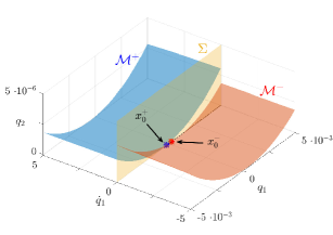
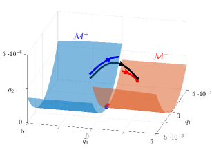
For model reduction in a piecewise smooth system, we consider separately the subregions of the phase space in which the system is smooth and apply the results of primary SSM theory separately in those subregions. In particular, we smoothly extend each subsystem locally across its domain boundary and locate primary, smooth SSMs anchored at fixed points in that boundary for the extended system. Such an SSM will only act as an invariant manifold for the full system over its original subregion of smooth dynamics. These various subsets of SSMs form the skeleton of an attractive set for the full system, with pieces of this skeleton connected by trajectories sliding off from them and converging to other pieces of the skeleton (see Fig. 1 and video in the Supplementary Material). The reduced dynamics across different SSM pieces then needs to be connected appropriately by a reduced-order model, as we detail below.
Refer to caption
(a)
Refer to caption
(b)
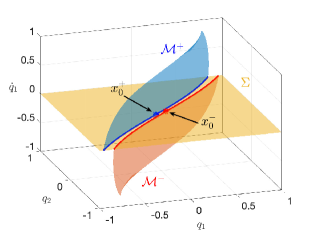
Figure 1: Reduced-order modeling strategy for piecewise smooth dynamical systems using primary SSMs. The plots depict a specific example, described in section 4 and reported here for motivation. Subfigure LABEL:sub@PWS_manifold represents the two primary SSMs, +superscript\mathcal{M}^{+} and superscript\mathcal{M}^{-}, anchored at their respective equilibrium points, x0+superscriptsubscript𝑥0x_{0}^{+} and x0superscriptsubscript𝑥0x_{0}^{-}, and separated by the switching surface ΣΣ\Sigma. Subfigure LABEL:sub@PWS_crossing exemplifies the crossing between two subregions. The black curve is the trajectory of the full system, which is approximated by the reduced dynamics (blue and red curves) lying on +superscript\mathcal{M}^{+} and superscript\mathcal{M}^{-}. The full solution quickly synchronizes with the reduced one, even though the latter involves a physical discontinuity.

In the following, we first introduce some terminology from the theory of piecewise smooth dynamical systems, then give a more thorough description of our construction of a reduced-order model.

2.1 Piecewise smooth systems

Let us consider the n𝑛n-dimensional dynamical system

𝐱˙=𝐟(𝐱;δ),𝐱n,δ,formulae-sequence˙𝐱𝐟𝐱𝛿formulae-sequence𝐱superscript𝑛𝛿\dot{\mathbf{x}}=\mathbf{f}(\mathbf{x};\delta),\quad\mathbf{x}\in\mathbb{R}^{n},\quad\delta\in\mathbb{R}, (1)

where 𝐱𝐱\mathbf{x} is the state vector and 𝐟(𝐱;δ)𝐟𝐱𝛿\mathbf{f}(\mathbf{x};\delta) is a nonlinear and non-smooth right-hand side, depending smoothly on the parameter δ𝛿\delta and the time t𝑡t, but not necessarily on the phase-space variable 𝐱𝐱\mathbf{x}. For simplicity, we assume 𝐟(𝐱;δ)𝐟𝐱𝛿\mathbf{f}(\mathbf{x};\delta) to be non-smooth across a single hypersurface ΣΣ\Sigma of dimension n1𝑛1n-1 that contains the origin 𝐱=𝟎𝐱0\mathbf{x}=\mathbf{0}. Namely, the phase space is split into two regions separated by the hypersurface ΣΣ\Sigma, and 𝐟(𝐱,δ)𝐟𝐱𝛿\mathbf{f}(\mathbf{x},\delta) is smooth within each of these regions.

The surface ΣΣ\Sigma is usually called a switching surface, defined by a scalar-valued switching function σ(𝐱)𝜎𝐱\sigma(\mathbf{x}) as

Σ={𝐱n:σ(𝐱)=0}Σconditional-set𝐱superscript𝑛𝜎𝐱0\Sigma=\left\{\mathbf{x}\in\mathbb{R}^{n}:\sigma(\mathbf{x})=0\right\} (2)

The phase space is then partitioned as n=Σ+ΣΣsuperscript𝑛superscriptΣΣsuperscriptΣ\mathbb{R}^{n}=\Sigma^{+}\cup\Sigma\cup\Sigma^{-}, where

Σ={𝐱n:σ(𝐱)<0},Σ+={𝐱n:σ(𝐱)>0}.superscriptΣconditional-set𝐱superscript𝑛𝜎𝐱0superscriptΣconditional-set𝐱superscript𝑛𝜎𝐱0\begin{array}[]{l}\Sigma^{-}=\left\{\mathbf{x}\in\mathbb{R}^{n}:\sigma(\mathbf{x})<0\right\},\\[6.0pt] \Sigma^{+}=\left\{\mathbf{x}\in\mathbb{R}^{n}:\sigma(\mathbf{x})>0\right\}.\end{array} (3)

The original piecewise smooth system (1) can now be written as

𝐱˙=𝐟(𝐱;δ)={𝐟+(𝐱;δ),𝐱Σ+,𝐟(𝐱;δ),𝐱Σ,˙𝐱𝐟𝐱𝛿casessuperscript𝐟𝐱𝛿𝐱superscriptΣsuperscript𝐟𝐱𝛿𝐱superscriptΣ\dot{\mathbf{x}}=\mathbf{f}(\mathbf{x};\delta)=\begin{cases}\mathbf{f}^{+}(\mathbf{x};\delta),&\mathbf{x}\in\Sigma^{+},\\ \mathbf{f}^{-}(\mathbf{x};\delta),&\mathbf{x}\in\Sigma^{-},\end{cases} (4)

where we assume that 𝐟±(𝐱;δ)superscript𝐟plus-or-minus𝐱𝛿\mathbf{f}^{\pm}(\mathbf{x};\delta) both extend to smooth functions of 𝐱𝐱\mathbf{x} in an open neighborhood of ΣΣ\Sigma. We also assume that

𝐟(𝐱;0)𝐟±(𝐱;0),𝐟(𝟎;0)=𝟎,0Re[Spect(D𝐱𝐟(𝟎;0)].\begin{array}[]{c}\mathbf{f}(\mathbf{x};0)\equiv\mathbf{f}^{\pm}(\mathbf{x};0),\quad\mathbf{f}(\mathbf{0};0)=\mathbf{0},\\[6.0pt] 0\notin\text{Re}[\text{Spect}(\text{D}_{\mathbf{x}}\mathbf{f}(\mathbf{0};0)].\end{array} (5)

In other words, for δ=0𝛿0\delta=0, the discontinuity of system (1) disappears and 𝐱=𝟎𝐱0\mathbf{x}=\mathbf{0} is a hyperbolic fixed point of (1), contained in ΣΣ\Sigma for this value of δ𝛿\delta. Note that by the theory developed by Filippov [11], the dynamics within ΣΣ\Sigma can be approximated by constructing a proper inclusion (see A.1).

We assume that trajectories intersecting ΣΣ\Sigma exhibit two possible behaviors:

Refer to caption
(a)
Refer to caption
(b)
Refer to caption
(c)
Refer to caption
(d)
Figure 2: The orbits can cross either from ΣsuperscriptΣ\Sigma^{-} to Σ+superscriptΣ\Sigma^{+} LABEL:sub@crossing_1 or from Σ+superscriptΣ\Sigma^{+} to ΣsuperscriptΣ\Sigma^{-} LABEL:sub@crossing_2. Alternatively, they can exhibit an attracting LABEL:sub@attractive_sliding or a repelling sliding mode LABEL:sub@repulsive_sliding.
  • 1.

    Crossing: the orbit crosses trough ΣΣ\Sigma if

    (σ𝐟+)(σ𝐟)>0 on Σ.𝜎superscript𝐟𝜎superscript𝐟0 on Σ(\nabla\sigma\cdot\mathbf{f}^{+})(\nabla\sigma\cdot\mathbf{f}^{-})>0\text{ on }\Sigma. (6)
  • 2.

    Sliding: the orbit slides along the switching surface if

    (σ𝐟+)(σ𝐟)<0 on Σ.𝜎superscript𝐟𝜎superscript𝐟0 on Σ(\nabla\sigma\cdot\mathbf{f}^{+})(\nabla\sigma\cdot\mathbf{f}^{-})<0\text{ on }\Sigma. (7)

    In the case of sliding, the vector field is tangent to the switching surface and can be expressed as a convex combination of 𝐟+superscript𝐟\mathbf{f}^{+} and 𝐟superscript𝐟\mathbf{f}^{-} along ΣΣ\Sigma. The switching surface ΣΣ\Sigma then either attracts or repels neighbouring trajectories, depending on the direction of the vector fields in Σ+superscriptΣ\Sigma^{+} and ΣsuperscriptΣ\Sigma^{-}, as seen in Fig. 2. In the former case, the solution generally evolves along the switching surface. In the latter case, a solution still exists, but it is not unique in forward time.

2.2 Model reduction strategy

We now outline a procedure which allows us to extend SSM-based model reduction to piecewise smooth systems. Our approach utilizes the primary SSMs constructed over slow modes existing on both sides of ΣΣ\Sigma by the theory of SSMs for smooth systems reviewed in A.2.

By our assumptions in section 2.1, for δ=0𝛿0\delta=0, system (1) has a hyperbolic fixed point at 𝐱=𝟎𝐱0\mathbf{x}=\mathbf{0}. Any nonresonant spectral subspace E0subscript𝐸0E_{0} of the linearized system at 𝐱=𝟎𝐱0\mathbf{x}=\mathbf{0} will then admit a unique, primary SSM, 0subscript0\mathcal{M}_{0}, under the addition to the nonlinear terms of 𝐟(𝐱;0)𝐟𝐱0\mathbf{f}(\mathbf{x};0). For δ0𝛿0\delta\neq 0 and small, hyperbolic fixed points will continue to exist 𝒪(δ)𝒪𝛿\mathcal{O}(\delta)-close to 𝐱=𝟎𝐱0\mathbf{x}=\mathbf{0} for the two ODEs 𝐱˙=𝐟±(𝐱;δ)˙𝐱superscript𝐟plus-or-minus𝐱𝛿\dot{\mathbf{x}}=\mathbf{f}^{\pm}(\mathbf{x};\delta) by the implicit function theorem. These fixed points, 𝐱0±(δ)superscriptsubscript𝐱0plus-or-minus𝛿\mathbf{x}_{0}^{\pm}(\delta), will have their own SSMs, δ±subscriptsuperscriptplus-or-minus𝛿\mathcal{M}^{\pm}_{\delta}, that are smooth, 𝒪(δ)𝒪𝛿\mathcal{O}(\delta) perturbations of 0subscript0\mathcal{M}_{0} by the smooth dependence of SSMs on parameters (Haller and Ponsioen [14]). As a consequence, the set δ=δ+δsubscript𝛿superscriptsubscript𝛿superscriptsubscript𝛿\mathcal{M}_{\delta}=\mathcal{M}_{\delta}^{+}\cup\mathcal{M}_{\delta}^{-} is a piecewise smooth attracting set for system (1).

We now recall the construction of a general SSM and its reduced dynamics from observable data (see Cenedese et al. [7], Axås et al. [1] for more detail). We seek the parametrization of the manifold \mathcal{M} as a graph over its a priori unknown tangent space T𝑇T\mathcal{M}, which is the image of the spectral subspace E𝐸E in the space of observables 𝐲n𝐲superscript𝑛\mathbf{y}\in\mathbb{R}^{n}. In particular, we approximate the manifold via a multi-variate Taylor expansion

𝐲(𝝃)=𝐌𝝃1:m=𝐕𝝃+𝐌2:m𝝃2:m,𝐲𝝃𝐌superscript𝝃:1𝑚𝐕𝝃subscript𝐌:2𝑚superscript𝝃:2𝑚\mathbf{y}(\boldsymbol{\xi})=\mathbf{M}\boldsymbol{\xi}^{1:m}=\mathbf{V}\boldsymbol{\xi}+\mathbf{M}_{2:m}\boldsymbol{\xi}^{2:m}, (8)

where 𝐌=[𝐕,𝐌2,,𝐌m]𝐌𝐕subscript𝐌2subscript𝐌𝑚\mathbf{M}=[\mathbf{V},\mathbf{M}_{2},...,\mathbf{M}_{m}], with 𝐌in×disubscript𝐌𝑖superscript𝑛subscript𝑑𝑖\mathbf{M}_{i}\in\mathbb{R}^{n\times d_{i}} and disubscript𝑑𝑖d_{i} refers to the number of d𝑑d-variate monomials at order i𝑖i. We refer to 𝝃=𝐕T𝐲𝝃superscript𝐕𝑇𝐲\boldsymbol{\xi}=\mathbf{V}^{T}\mathbf{y} as reduced coordinates, where the columns of the matrix 𝐕n×d𝐕superscript𝑛𝑑\mathbf{V}\in\mathbb{R}^{n\times d} are orthonormal vectors that span T𝑇T\mathcal{M}. The notation ()l:rsuperscript:𝑙𝑟(\cdot)^{l:r} refers to the vector containing all monomials composed of the entries of the vector ()(\cdot), with monomials ranging from l𝑙l to r𝑟r. For instance, if 𝝃=[ξ1ξ2]T𝝃superscriptdelimited-[]subscript𝜉1subscript𝜉2𝑇\boldsymbol{\xi}=[\xi_{1}\xi_{2}]^{T}, then

𝝃2:3=[ξ12,ξ1ξ2,ξ22,ξ13,ξ12ξ2,ξ1ξ22,ξ23]T.superscript𝝃:23superscriptsuperscriptsubscript𝜉12subscript𝜉1subscript𝜉2superscriptsubscript𝜉22superscriptsubscript𝜉13superscriptsubscript𝜉12subscript𝜉2subscript𝜉1superscriptsubscript𝜉22superscriptsubscript𝜉23T\boldsymbol{\xi}^{2:3}=[\xi_{1}^{2},\,\xi_{1}\xi_{2},\,\xi_{2}^{2},\,\xi_{1}^{3},\,\xi_{1}^{2}\xi_{2},\,\xi_{1}\xi_{2}^{2},\,\xi_{2}^{3}]^{\mathrm{T}}.

Learning \mathcal{M} from a set of training data {𝐲j}subscript𝐲𝑗\{\mathbf{y}_{j}\} in the observable space means finding the optimal matrix 𝐌superscript𝐌\mathbf{M}^{\ast}, such that

(𝐕,𝐌)=argmin𝐕,𝐌2:mj𝐲j𝐕𝐕T𝐲j𝐌2:m(𝐕T𝐲j)2:m,superscript𝐕superscript𝐌𝐕subscript𝐌:2𝑚subscript𝑗normsubscript𝐲𝑗superscript𝐕𝐕𝑇subscript𝐲𝑗subscript𝐌:2𝑚superscriptsuperscript𝐕𝑇subscript𝐲𝑗:2𝑚\left(\mathbf{V^{\ast}},\mathbf{M}^{\ast}\right)=\underset{\mathbf{V},\mathbf{M}_{2:m}}{\arg\min}\sum_{j}\Big{\|}\mathbf{y}_{j}-\mathbf{V}\mathbf{V}^{T}\mathbf{y}_{j}-\mathbf{M}_{2:m}(\mathbf{V}^{T}\mathbf{y}_{j})^{2:m}\Big{\|}, (9)

subject to the constraints

𝐕𝐕T=𝕀,𝐕𝐌2:m=𝟎.formulae-sequencesuperscript𝐕𝐕𝑇𝕀subscript𝐕𝐌:2𝑚0\mathbf{V}\mathbf{V}^{T}=\mathbb{I},\quad\mathbf{V}\mathbf{M}_{2:m}=\mathbf{0}. (10)

The dynamics on the SSM in the reduced coordinates 𝝃𝝃\boldsymbol{\xi} can then be approximated as

𝝃˙=𝐑𝝃1:r,˙𝝃𝐑superscript𝝃:1𝑟\dot{\boldsymbol{\xi}}=\mathbf{R}\boldsymbol{\xi}^{1:r}, (11)

where the elements of 𝐑d:d1:r𝐑superscript:𝑑subscript𝑑:1𝑟\mathbf{R}\in\mathbb{R}^{d:d_{1:r}} are found by solving the minimization problem

𝐑=argmin𝐑𝝃˙j𝐑𝝃j1:r.superscript𝐑𝐑normsubscript˙𝝃𝑗𝐑superscriptsubscript𝝃𝑗:1𝑟\mathbf{R}^{\ast}=\underset{\mathbf{R}}{\arg\min}\Big{\|}\dot{\boldsymbol{\xi}}_{j}-\mathbf{R}\boldsymbol{\xi}_{j}^{1:r}\Big{\|}. (12)

In the present work, we assume to know a priori the model of the system that generates the data 𝐲jsubscript𝐲𝑗\mathbf{y}_{j}, as well as the linear parts of the parametrization (8) and reduced dynamics (11), as in Cenedese et al. [9]. More specifically, in the piecewise smooth context, we suppose that the governing equations, the domains Σ±superscriptΣplus-or-minus\Sigma^{\pm}, and the switching function σ(𝐱)𝜎𝐱\sigma(\mathbf{x}) defining ΣΣ\Sigma are known.

With these ingredients, we will use the smoothly extended versions of the right-hand sides 𝐟±(𝐱;δ)superscript𝐟plus-or-minus𝐱𝛿\mathbf{f}^{\pm}(\mathbf{x};\delta) to generate training data {𝐲j±}superscriptsubscript𝐲𝑗plus-or-minus\{\mathbf{y}_{j}^{\pm}\} from both ODEs 𝐱˙=𝐟±(𝐱;δ)˙𝐱superscript𝐟plus-or-minus𝐱𝛿\dot{\mathbf{x}}=\mathbf{f}^{\pm}(\mathbf{x};\delta) in a neighborhood of the switching surface. We then construct the SSMs, δ±subscriptsuperscriptplus-or-minus𝛿\mathcal{M}^{\pm}_{\delta}, separately, but only keep their subsets falling in the domains Σ±superscriptΣplus-or-minus\Sigma^{\pm}, respectively. Our reduced-order will then switch between the reduced dynamics of δ±superscriptsubscript𝛿plus-or-minus\mathcal{M}_{\delta}^{\pm} based on appropriately reduced switching conditions that we will discuss in our upcoming examples.

3 Example 1: Shaw-Pierre model with friction

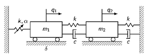
We add friction to a modified version of the mechanical system studied by Shaw and Pierre [28], as introduced in Haller and Ponsioen [14]. The resulting system is sketched in Fig. 3.
Refer to caption
(a)
Refer to caption
(b)
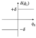
Figure 3: Two-degree-of-freedom modified Shaw-Pierre mechanical system with friction. LABEL:sub@mechanical_system System geometry. LABEL:sub@friction_law Coulomb friction law added to the first mass.

Dry friction is modelled via the classical Coulomb’s law (Leine and Nijmeijer [22]), where the static friction coefficient δ𝛿\delta (active when q˙1=0subscript˙𝑞10\dot{q}_{1}=0) is equal to the dynamic one (valid when q˙10subscript˙𝑞10\dot{q}_{1}\neq 0). We now follow the procedure outlined in section 2 for the computation of a reduced order model for this piecewise smooth system.

Non-smooth formulation

The equations of motion of the system in Fig. 3 are

(m100m2)(q¨1q¨2)+(ccc2c)(q˙1q˙2)matrixsubscript𝑚100subscript𝑚2matrixsubscript¨𝑞1subscript¨𝑞2matrix𝑐𝑐𝑐2𝑐matrixsubscript˙𝑞1subscript˙𝑞2\displaystyle\begin{pmatrix}m_{1}&0\\ 0&m_{2}\end{pmatrix}\begin{pmatrix}\ddot{q}_{1}\\ \ddot{q}_{2}\end{pmatrix}+\begin{pmatrix}c&-c\\ -c&2c\end{pmatrix}\begin{pmatrix}\dot{q}_{1}\\ \dot{q}_{2}\end{pmatrix} (13)
+(2kkk2k)(q1q2)+(αq130)=(δ(q˙1)m1g0),matrix2𝑘𝑘𝑘2𝑘matrixsubscript𝑞1subscript𝑞2matrix𝛼superscriptsubscript𝑞130matrix𝛿subscript˙𝑞1subscript𝑚1𝑔0\displaystyle\quad+\begin{pmatrix}2k&-k\\ -k&2k\end{pmatrix}\begin{pmatrix}q_{1}\\ q_{2}\end{pmatrix}+\begin{pmatrix}-\alpha q_{1}^{3}\\ 0\end{pmatrix}=\begin{pmatrix}-\delta({\dot{q}_{1}})m_{1}g\\ 0\end{pmatrix},

where g𝑔g denotes the constant of gravity. In the following, δ=δ(q˙1)g𝛿𝛿subscript˙𝑞1𝑔\delta=\delta(\dot{q}_{1})g. With the notation x1=q1subscript𝑥1subscript𝑞1x_{1}=q_{1}, x2=q˙1subscript𝑥2subscript˙𝑞1x_{2}=\dot{q}_{1}, x3=q2subscript𝑥3subscript𝑞2x_{3}=q_{2} and x4=q˙2subscript𝑥4subscript˙𝑞2x_{4}=\dot{q}_{2}, we can rewrite eq.(13) as a first-order system of ODEs

𝐱˙=𝐀0𝐱+𝐟𝐧𝐥𝐟δ,˙𝐱minus-or-plussubscript𝐀0𝐱subscript𝐟𝐧𝐥subscript𝐟𝛿\dot{\mathbf{x}}=\mathbf{A}_{0}\mathbf{x}+\mathbf{f_{nl}}\mp\,\mathbf{f_{\delta}}, (14)

with

𝐀0=(01002km1cm1km1cm10001km2cm22km22cm2),subscript𝐀0matrix01002𝑘subscript𝑚1𝑐subscript𝑚1𝑘subscript𝑚1𝑐subscript𝑚10001𝑘subscript𝑚2𝑐subscript𝑚22𝑘subscript𝑚22𝑐subscript𝑚2\displaystyle\mathbf{A}_{0}=\begin{pmatrix}0&1&0&0\\ -\frac{2k}{m_{1}}&-\frac{c}{m_{1}}&\frac{k}{m_{1}}&\frac{c}{m_{1}}\\ 0&0&0&1\\ \frac{k}{m_{2}}&\frac{c}{m_{2}}&-\frac{2k}{m_{2}}&-\frac{2c}{m_{2}}\end{pmatrix},
𝐟𝐧𝐥=(0,αm1x13,0,0)T,𝐟δ=(0,δ,0,0)T.formulae-sequencesubscript𝐟𝐧𝐥superscriptmatrix0𝛼subscript𝑚1superscriptsubscript𝑥1300Tsubscript𝐟𝛿superscriptmatrix0𝛿00T\displaystyle\mathbf{f_{nl}}=\begin{pmatrix}0,-\frac{\alpha}{m_{1}}x_{1}^{3},0,0\end{pmatrix}^{\mathrm{T}},\quad\mathbf{f_{\delta}}=\begin{pmatrix}0,\delta,0,0\end{pmatrix}^{\mathrm{T}}.

The sign of the velocity x2subscript𝑥2x_{2} of the first mass decides whether the friction force is positive or negative, hence this velocity defines the switching function

σ(𝐱)=x2=q˙1.𝜎𝐱subscript𝑥2subscript˙𝑞1\sigma(\mathbf{x})=x_{2}=\dot{q}_{1}. (15)

Therefore, we have the splitting 4=Σ+ΣΣsuperscript4superscriptΣΣsuperscriptΣ\mathbb{R}^{4}=\Sigma^{+}\cup\Sigma\cup\Sigma^{-}, where

Σ±={𝐱4:sign(σ(𝐱))=±1}.superscriptΣplus-or-minusconditional-set𝐱superscript4sign𝜎𝐱plus-or-minus1\begin{array}[]{l}\Sigma^{\pm}=\left\{\mathbf{x}\in\mathbb{R}^{4}:\text{sign}(\sigma(\mathbf{x}))=\pm 1\right\}.\end{array} (16)

The piecewise smooth system (1) is here specifically defined as

𝐱˙˙𝐱\displaystyle\dot{\mathbf{x}} =𝐟±(𝐱;δ)absentsuperscript𝐟plus-or-minus𝐱𝛿\displaystyle=\mathbf{f}^{\pm}(\mathbf{x};\delta) (17)
=(x22km1x1cm1x2+km1x3+cm1x4αm1x13δx4km2x1+cm2x22km2x32cm2x4).absentmatrixsubscript𝑥2minus-or-plus2𝑘subscript𝑚1subscript𝑥1𝑐subscript𝑚1subscript𝑥2𝑘subscript𝑚1subscript𝑥3𝑐subscript𝑚1subscript𝑥4𝛼subscript𝑚1superscriptsubscript𝑥13𝛿subscript𝑥4𝑘subscript𝑚2subscript𝑥1𝑐subscript𝑚2subscript𝑥22𝑘subscript𝑚2subscript𝑥32𝑐subscript𝑚2subscript𝑥4\displaystyle=\begin{pmatrix}\displaystyle x_{2}\\ \displaystyle-\frac{2k}{m_{1}}x_{1}-\frac{c}{m_{1}}x_{2}+\frac{k}{m_{1}}x_{3}+\frac{c}{m_{1}}x_{4}-\frac{\alpha}{m_{1}}x_{1}^{3}\mp\delta\\ x_{4}\\ \displaystyle\frac{k}{m_{2}}x_{1}+\frac{c}{m_{2}}x_{2}-\frac{2k}{m_{2}}x_{3}-\frac{2c}{m_{2}}x_{4}\end{pmatrix}.

Given that σ=(0,1,0,0)T𝜎superscript0100T\nabla\sigma=(0,1,0,0)^{\mathrm{T}}, a crossing of ΣΣ\Sigma at a point 𝐱Σ𝐱Σ\mathbf{x}\in\Sigma takes place if σ𝐟+𝜎superscript𝐟\nabla\sigma\cdot\mathbf{f}^{+} and σ𝐟>0𝜎superscript𝐟0\nabla\sigma\cdot\mathbf{f}^{-}>0 have the same nonzero sign at 𝐱𝐱\mathbf{x}, i.e.,

{2km1x1+km1x3+cm1x4αm1x13>δ,2km1x1+km1x3+cm1x4αm1x13>δ,orcases2𝑘subscript𝑚1subscript𝑥1𝑘subscript𝑚1subscript𝑥3𝑐subscript𝑚1subscript𝑥4𝛼subscript𝑚1superscriptsubscript𝑥13𝛿otherwise2𝑘subscript𝑚1subscript𝑥1𝑘subscript𝑚1subscript𝑥3𝑐subscript𝑚1subscript𝑥4𝛼subscript𝑚1superscriptsubscript𝑥13𝛿otherwiseor\displaystyle\begin{cases}\displaystyle-\frac{2k}{m_{1}}x_{1}+\frac{k}{m_{1}}x_{3}+\frac{c}{m_{1}}x_{4}-\frac{\alpha}{m_{1}}x_{1}^{3}>\delta,\vspace{0.3cm}\\ \displaystyle-\frac{2k}{m_{1}}x_{1}+\frac{k}{m_{1}}x_{3}+\frac{c}{m_{1}}x_{4}-\frac{\alpha}{m_{1}}x_{1}^{3}>-\delta,\end{cases}\text{or} (18)
{2km1x1+km1x3+cm1x4αm1x13<δ,2km1x1+km1x3+cm1x4αm1x13<δ.cases2𝑘subscript𝑚1subscript𝑥1𝑘subscript𝑚1subscript𝑥3𝑐subscript𝑚1subscript𝑥4𝛼subscript𝑚1superscriptsubscript𝑥13𝛿otherwise2𝑘subscript𝑚1subscript𝑥1𝑘subscript𝑚1subscript𝑥3𝑐subscript𝑚1subscript𝑥4𝛼subscript𝑚1superscriptsubscript𝑥13𝛿otherwise\displaystyle\begin{cases}\displaystyle-\frac{2k}{m_{1}}x_{1}+\frac{k}{m_{1}}x_{3}+\frac{c}{m_{1}}x_{4}-\frac{\alpha}{m_{1}}x_{1}^{3}<\delta,\vspace{0.3cm}\\ \displaystyle-\frac{2k}{m_{1}}x_{1}+\frac{k}{m_{1}}x_{3}+\frac{c}{m_{1}}x_{4}-\frac{\alpha}{m_{1}}x_{1}^{3}<-\delta.\end{cases}

Attracting sliding motion along ΣΣ\Sigma ensues when

|2km1x1+km1x3+cm1x4αm1x13|<δ.2𝑘subscript𝑚1subscript𝑥1𝑘subscript𝑚1subscript𝑥3𝑐subscript𝑚1subscript𝑥4𝛼subscript𝑚1superscriptsubscript𝑥13𝛿\Big{|}-\frac{2k}{m_{1}}x_{1}+\frac{k}{m_{1}}x_{3}+\frac{c}{m_{1}}x_{4}-\frac{\alpha}{m_{1}}x_{1}^{3}\Big{|}<\delta. (19)

Inside the switching surface ΣΣ\Sigma, the first mass is in the state of sticking and the second mass acts as a linear harmonic oscillator, i.e., we have

𝐱˙=(00x4km2x12km2x32cm2x4),𝐱Σ.formulae-sequence˙𝐱matrix00subscript𝑥4𝑘subscript𝑚2subscript𝑥12𝑘subscript𝑚2subscript𝑥32𝑐subscript𝑚2subscript𝑥4𝐱Σ\dot{\mathbf{x}}=\begin{pmatrix}0\\ 0\\ x_{4}\\ \frac{k}{m_{2}}x_{1}-\frac{2k}{m_{2}}x_{3}-\frac{2c}{m_{2}}x_{4}\end{pmatrix},\quad\mathbf{x}\in\Sigma. (20)

The conditions for repulsive sliding mode are

{2km1x1+km1x3+cm1x4αm1x13>δ,2km1x1+km1x3+cm1x4αm1x13<δ,cases2𝑘subscript𝑚1subscript𝑥1𝑘subscript𝑚1subscript𝑥3𝑐subscript𝑚1subscript𝑥4𝛼subscript𝑚1superscriptsubscript𝑥13𝛿otherwise2𝑘subscript𝑚1subscript𝑥1𝑘subscript𝑚1subscript𝑥3𝑐subscript𝑚1subscript𝑥4𝛼subscript𝑚1superscriptsubscript𝑥13𝛿otherwise\begin{cases}\displaystyle-\frac{2k}{m_{1}}x_{1}+\frac{k}{m_{1}}x_{3}+\frac{c}{m_{1}}x_{4}-\frac{\alpha}{m_{1}}x_{1}^{3}>\delta\vspace{0.3cm},\\ \displaystyle-\frac{2k}{m_{1}}x_{1}+\frac{k}{m_{1}}x_{3}+\frac{c}{m_{1}}x_{4}-\frac{\alpha}{m_{1}}x_{1}^{3}<-\delta,\end{cases} (21)

which cannot be satisfied for any 𝐱Σ𝐱Σ\mathbf{x}\in\Sigma. As a consequence, the Shaw-Pierre system with friction exhibits either crossing or attracting sliding (or sticking) behavior.

We will simulate the behavior of the system with the parameter values used by Shaw and Pierre [28] and Haller and Ponsioen [14],

m=1,c=0.3,k=1,α=0.5,formulae-sequence𝑚1formulae-sequence𝑐0.3formulae-sequence𝑘1𝛼0.5m=1,\quad c=0.3,\quad k=1,\quad\alpha=0.5,

and will consider a range of δ𝛿\delta values in our analysis.

Analysis of the linearized system

The two different dynamical systems defined in (17) have their own fixed points and smooth SSMs anchored at them. The fixed points are defined by

𝐱0±=(q0±012q0±0),superscriptsubscript𝐱0plus-or-minusmatrixsuperscriptsubscript𝑞0plus-or-minus012superscriptsubscript𝑞0plus-or-minus0\displaystyle\mathbf{x}_{0}^{\pm}=\begin{pmatrix}q_{0}^{\pm}\\ 0\\ \frac{1}{2}q_{0}^{\pm}\\ 0\end{pmatrix}, (22)
q0±=±δ+δ2+13δ+δ2+13.superscriptsubscript𝑞0plus-or-minusminus-or-plusplus-or-minus3𝛿superscript𝛿213𝛿superscript𝛿21\displaystyle q_{0}^{\pm}=\pm\sqrt[3]{-\delta+\sqrt{\delta^{2}+1}}\mp\sqrt[3]{\delta+\sqrt{\delta^{2}+1}}.

We shift coordinates so that the origin in the two cases coincides with 𝐱0±superscriptsubscript𝐱0plus-or-minus\mathbf{x}_{0}^{\pm}, respectively:

ξ±=𝐱𝐱0±=(q1q0±q˙1q212q0±q˙2).superscript𝜉plus-or-minus𝐱superscriptsubscript𝐱0plus-or-minusmatrixsubscript𝑞1superscriptsubscript𝑞0plus-or-minussubscript˙𝑞1subscript𝑞212superscriptsubscript𝑞0plus-or-minussubscript˙𝑞2\mathbf{\xi}^{\pm}=\mathbf{x}-\mathbf{x}_{0}^{\pm}=\begin{pmatrix}q_{1}-q_{0}^{\pm}\\ \dot{q}_{1}\\ q_{2}-\frac{1}{2}q_{0}^{\pm}\\ \dot{q}_{2}\end{pmatrix}. (23)

In these coordinates, system (17) becomes

ξ˙±=𝐀~0ξ±+𝐟𝐧𝐥𝐈𝐈(ξ±)+𝐟𝐧𝐥𝐈𝐈𝐈(ξ±)+𝐟0,superscript˙𝜉plus-or-minussubscript~𝐀0superscript𝜉plus-or-minussuperscriptsubscript𝐟𝐧𝐥𝐈𝐈superscript𝜉plus-or-minussuperscriptsubscript𝐟𝐧𝐥𝐈𝐈𝐈superscript𝜉plus-or-minussubscript𝐟0\dot{\mathbf{\xi}}^{\pm}=\mathbf{\tilde{A}}_{0}\mathbf{\xi}^{\pm}+\mathbf{f_{nl}^{II}}(\mathbf{\xi}^{\pm})+\mathbf{f_{nl}^{III}}(\mathbf{\xi}^{\pm})+\mathbf{f}_{0}, (24)

with

𝐀~0=(0100232(q0±)20.310.3000110.320.6),subscript~𝐀0matrix0100232superscriptsuperscriptsubscript𝑞0plus-or-minus20.310.3000110.320.6\displaystyle\mathbf{\tilde{A}}_{0}=\begin{pmatrix}0&1&0&0\\ -2-\frac{3}{2}{(q_{0}^{\pm})}^{2}&-0.3&1&0.3\\ 0&0&0&1\\ 1&0.3&-2&-0.6\end{pmatrix}, (25)
𝐟𝐧𝐥𝐈𝐈(ξ±)=(0,32q0±(ξ1±)2,0,0)T,superscriptsubscript𝐟𝐧𝐥𝐈𝐈superscript𝜉plus-or-minussuperscriptmatrix032superscriptsubscript𝑞0plus-or-minussuperscriptsuperscriptsubscript𝜉1plus-or-minus200T\displaystyle\mathbf{f_{nl}^{II}}(\mathbf{\xi}^{\pm})=\begin{pmatrix}0,-\frac{3}{2}q_{0}^{\pm}\left(\xi_{1}^{\pm}\right)^{2},0,0\end{pmatrix}^{\mathrm{T}},
𝐟𝐧𝐥𝐈𝐈𝐈(ξ±)=(0,12(ξ1±)3,0,0)T,superscriptsubscript𝐟𝐧𝐥𝐈𝐈𝐈superscript𝜉plus-or-minussuperscriptmatrix012superscriptsuperscriptsubscript𝜉1plus-or-minus300T\displaystyle\mathbf{f_{nl}^{III}}(\mathbf{\xi}^{\pm})=\begin{pmatrix}0,-\frac{1}{2}\left(\xi_{1}^{\pm}\right)^{3},0,0\end{pmatrix}^{\mathrm{T}},
𝐟0=(0,32q0±12(q0±)3δ,0,0)T.subscript𝐟0superscriptmatrix0minus-or-plus32superscriptsubscript𝑞0plus-or-minus12superscriptsuperscriptsubscript𝑞0plus-or-minus3𝛿00T\displaystyle\mathbf{f}_{0}=\begin{pmatrix}0,-\frac{3}{2}q_{0}^{\pm}-\frac{1}{2}(q_{0}^{\pm})^{3}\mp\delta,0,0\end{pmatrix}^{\mathrm{T}}.

The matrix 𝐀~0subscript~𝐀0\mathbf{\tilde{A}}_{0} is unaffected by the sign choice in q0±superscriptsubscript𝑞0plus-or-minusq_{0}^{\pm}, therefore both cases have the same spectral properties and hence the same spectral subspaces.
The eigenvalues of 𝐀~0subscript~𝐀0\mathbf{\tilde{A}}_{0} for δ=101𝛿superscript101\delta=10^{-1} are

λ1,2=0.0741±i 1.0027,λ3,4=0.3759±i 1.6812,subscript𝜆12plus-or-minus0.0741𝑖1.0027subscript𝜆34plus-or-minus0.3759𝑖1.6812\begin{array}[]{l}\lambda_{1,2}=-0.0741\pm i\,1.0027,\\ \lambda_{3,4}=-0.3759\pm i\,1.6812,\end{array}

whose eigenvectors give rise to two two-dimensional real invariant subspaces, E1subscript𝐸1E_{1} and E2subscript𝐸2E_{2}.

3.1 Computation of SSMs.

According to the definition given in A.2, the relative spectral quotients of E1subscript𝐸1E_{1} and E2subscript𝐸2E_{2} are

σ(E1)=Int[Reλ3,4Reλ1,2]=5.𝜎subscript𝐸1Intdelimited-[]Resubscript𝜆34Resubscript𝜆125\begin{array}[]{l}\sigma(E_{1})=\text{Int}\left[\frac{\text{Re}\,\lambda_{3,4}}{\text{Re}\,\lambda_{1,2}}\right]=5.\end{array} (26)

Changing the friction coefficient δ𝛿\delta has a mild effect on the eigenvalues and hence the spectral quotients will not change for the range of friction coefficients studied here. Considerations about the existence and uniqueness of the SSMs in the positive and negative cases are exactly the same, as they share the same linearized dynamics, even though they are anchored at different points. The nonlinear contribution of the spring 𝐟𝐧𝐥subscript𝐟𝐧𝐥\mathbf{f_{nl}} is an autonomous term that is analytic on the whole phase space.

Based on these facts, the results in Haller and Ponsioen [14] guarantee the existence and uniqueness of the slow two-dimensional SSM, 1(0)subscript10\mathcal{M}_{1}(0), because the required nonresonance conditions among the eigenvalues are satisfied up to order σ(E1)𝜎subscript𝐸1\sigma(E_{1}) (see Haller and Ponsioen [14] for details). Therefore, we can state that the analytic SSM 1(0)subscript10\mathcal{M}_{1}(0) exists and it is unique among all 𝒞6superscript𝒞6\mathcal{C}^{6} invariant manifolds tangent to E1subscript𝐸1E_{1} at the origin. We introduce coordinates aligned with E1subscript𝐸1E_{1} and E2subscript𝐸2E_{2} by letting

𝝃±=𝐕𝜼±,superscript𝝃plus-or-minus𝐕superscript𝜼plus-or-minus\boldsymbol{\xi}^{\pm}=\mathbf{V}\boldsymbol{\eta}^{\pm}, (27)

where

𝜼±=(𝐲±,𝐳±)E1×E2,superscript𝜼plus-or-minussuperscript𝐲plus-or-minussuperscript𝐳plus-or-minussubscript𝐸1subscript𝐸2\boldsymbol{\eta}^{\pm}=(\mathbf{y}^{\pm},\mathbf{z}^{\pm})\in E_{1}\times E_{2},

and 𝐕𝐕\mathbf{V} is the matrix whose columns are the eigenvectors of 𝐀~𝟎subscript~𝐀0\mathbf{\tilde{A}_{0}}. The reduced coordinates 𝐲±superscript𝐲plus-or-minus\mathbf{y}^{\pm} act as the master variables over which we seek the slow SSM as a graph.
We report the analytical computation of the SSM in A.3.

3.2 Combination of SSMs and the switching surface.

We now restrict the SSMs constructed at 𝐱0±superscriptsubscript𝐱0plus-or-minus\mathbf{x}_{0}^{\pm} to their region of validity imposed by condition (16). The resulting restricted SSMs are separated by the switching surface ΣΣ\Sigma, as seen in Fig. 4.

Refer to caption
Figure 4: The two primary SSMs +superscript\mathcal{M}^{+} and superscript\mathcal{M}^{-}, separated by the switching surface ΣΣ\Sigma, for δ=101𝛿superscript101\delta=10^{-1}.

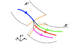
As the two pieces of primary SSMs form an attracting set for the full system, the dynamics restricted to them provides a reduced-order model for nearby initial conditions. We now describe how we connect the dynamics across the different SSM pieces when a trajectory hits the switching surface and satisfies the crossing condition (18). In this scenario, coming from one SSM, we need a new initial condition lying on the other one. By Fig. 6, the intersection between the incoming trajectory and the switching surface (blue dot in Fig. 6a) is associated to a set of both reduced 𝐲±=(y1±,y2±)Tsuperscript𝐲plus-or-minussuperscriptsuperscriptsubscript𝑦1plus-or-minussuperscriptsubscript𝑦2plus-or-minusT\mathbf{y}^{\pm}=\left(y_{1}^{\pm},y_{2}^{\pm}\right)^{\mathrm{T}} and observable 𝐱=(q1,q˙1,q2,q˙2)T𝐱superscriptsubscript𝑞1subscript˙𝑞1subscript𝑞2subscript˙𝑞2T\mathbf{x}=\left(q_{1},\dot{q}_{1},q_{2},\dot{q}_{2}\right)^{\mathrm{T}} coordinates. We then exploit the relationship between the two sets of reduced coordinates for the two SSMs to find the new initial condition (red dot in Fig. 6a) as

(y1y2)=(y1+y2+)+𝐕121(𝐱0+𝐱0),matrixsuperscriptsubscript𝑦1superscriptsubscript𝑦2matrixsuperscriptsubscript𝑦1superscriptsubscript𝑦2subscriptsuperscript𝐕112superscriptsubscript𝐱0superscriptsubscript𝐱0\begin{pmatrix}y_{1}^{-}\\ y_{2}^{-}\end{pmatrix}=\begin{pmatrix}y_{1}^{+}\\ y_{2}^{+}\end{pmatrix}+\mathbf{V}^{-1}_{12}(\mathbf{x}_{0}^{+}-\mathbf{x}_{0}^{-}), (28)

where the rectangular matrix 𝐕121subscriptsuperscript𝐕112\mathbf{V}^{-1}_{12} contains the first two rows of 𝐕1superscript𝐕1\mathbf{V}^{-1}. Coming from +superscript\mathcal{M}^{+}, the new initial condition (y1,y2)superscriptsubscript𝑦1superscriptsubscript𝑦2(y_{1}^{-},y_{2}^{-}) on superscript\mathcal{M}^{-} according to eq. (28) does not lie in the intersection between the superscript\mathcal{M}^{-} and the switching surface. As a consequence, all physical variables experience a discontinuity while crossing from one SSM to the other. Discontinuities in the solution are unavoidable, but one can investigate further strategies in order to enforce physical consistency for specific variables, as seen in Fig. 6.
Refer to caption
(a)
Refer to caption
(b)
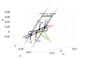
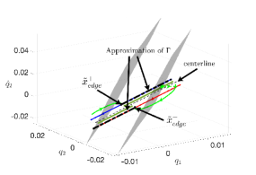
Figure 5: The invariant curve ΓΓ\Gamma of the Poincaré map for the Shaw-Pierre model with friction presents a discontinuity close to the origin. The grey surfaces delimit the region where sticking occurs and contain the two fixed points x0±superscriptsubscript𝑥0plus-or-minusx_{0}^{\pm}. LABEL:sub@edges_full_scaled: xedge±subscriptsuperscript𝑥plus-or-minus𝑒𝑑𝑔𝑒x^{\pm}_{edge} are the iterates of the configurations closest to the sticking (green squares), according to the full order model. LABEL:sub@edges_reduced_scaled: an approximation of the invariant curve ΓΓ\Gamma is derived as a portion of the blue and red lines, namely the intersection of the positive and negative SSMs with the switching surface, where x~edge±superscriptsubscript~𝑥𝑒𝑑𝑔𝑒plus-or-minus\tilde{x}_{edge}^{\pm} are defined by the reduced-order model.
Refer to caption
(a)
Refer to caption
(b)
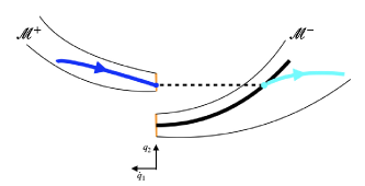
Figure 6: Different strategies for the computation of the new initial condition of the reduced dynamics across the switching surface ΣΣ\Sigma. The orange lines represent the intersection of the SSMs with the ΣΣ\Sigma. When a trajectory on one SSM (blue line) hits the switching surface, the projection of the intersection point onto the new SSM according to eq. (28) (red dot) represents a new initial condition. Alternatively, we can enforce that the new initial condition lies on the switching surface, minimizing the different of all physical variables across the jump (green dot) or ensuring the continuity of q1subscript𝑞1q_{1} (purple dot). If we require that both q1subscript𝑞1q_{1} and q2subscript𝑞2q_{2} are continuous (light blue dot), then the new initial condition lands far from the switching surface. The black line in LABEL:sub@ic_strategies2 depicts the set of points on the manifold superscript\mathcal{M}^{-} with the same value of q1subscript𝑞1q_{1} as the final point of the blue trajectory on +superscript\mathcal{M}^{+}.

Studying the reduced dynamics according to these different choices, we find that the initial condition defined by (28) tracks the full solution most effectively (see A.3.2). Therefore, we will use this matching scheme for initial conditions in the following.

3.3 Poincaré map and invariant set

We now seek an actual attractor (i.e., a closed invariant set with an open domain of attraction) near the locally invariant, attracting set +superscriptsuperscript\mathcal{M}^{+}\cup\mathcal{M}^{-}. To this end, we consider a set of initial conditions around the intersection of ±superscriptplus-or-minus\mathcal{M}^{\pm} with the switching surface in the (q1,q2,q˙2)subscript𝑞1subscript𝑞2subscript˙𝑞2(q_{1},q_{2},\dot{q}_{2}) space. Recording the subsequent crossing of trajectories through ΣΣ\Sigma defines a Poincaré map, which turns out to have an invariant curve ΓΓ\Gamma with a discontinuity close to the origin (green straight piecewise continuous line in Fig. 5). The two segments of this invariant curve lie close to the intersection of ±superscriptplus-or-minus\mathcal{M}^{\pm} with ΣΣ\Sigma (blue and red lines) on either side of the origin. The points at the discontinuity of ΓΓ\Gamma are denoted xedge±subscriptsuperscript𝑥plus-or-minus𝑒𝑑𝑔𝑒x^{\pm}_{edge}. They arise from the states closest to the sticking regime (green squares in 5a). In these states, the sum of forces from the springs and dampers are almost equal to the static friction force, but enough to induce crossing. The invariant curve ΓΓ\Gamma and xedge±subscriptsuperscript𝑥plus-or-minus𝑒𝑑𝑔𝑒x^{\pm}_{edge} have been computed integrating the full model, but they can be directly approximated from the reduced-order model (see A.3.3).

3.4 Non-autonomous problem

Under small periodic external force applied to the mass m1subscript𝑚1m_{1}, system (1) becomes

(m100m2)(q¨1q¨2)+(ccc2c)(q˙1q˙2)+(2kkk2k)(q1q2)matrixsubscript𝑚100subscript𝑚2matrixsubscript¨𝑞1subscript¨𝑞2matrix𝑐𝑐𝑐2𝑐matrixsubscript˙𝑞1subscript˙𝑞2matrix2𝑘𝑘𝑘2𝑘matrixsubscript𝑞1subscript𝑞2\displaystyle\begin{pmatrix}m_{1}&0\\ 0&m_{2}\end{pmatrix}\begin{pmatrix}\ddot{q}_{1}\\ \ddot{q}_{2}\end{pmatrix}+\begin{pmatrix}c&-c\\ -c&2c\end{pmatrix}\begin{pmatrix}\dot{q}_{1}\\ \dot{q}_{2}\end{pmatrix}+\begin{pmatrix}2k&-k\\ -k&2k\end{pmatrix}\begin{pmatrix}q_{1}\\ q_{2}\end{pmatrix} (29)
+(αq130)±(δm10)=ϵ12(11)cosΩt,plus-or-minusmatrix𝛼superscriptsubscript𝑞130matrix𝛿subscript𝑚10italic-ϵ12matrix11Ω𝑡\displaystyle+\begin{pmatrix}-\alpha q_{1}^{3}\\ 0\end{pmatrix}\pm\begin{pmatrix}\delta m_{1}\\ 0\end{pmatrix}=\epsilon\frac{1}{\sqrt{2}}\begin{pmatrix}1\\ 1\end{pmatrix}\cos{\Omega t},

where 0ϵ<<10italic-ϵmuch-less-than10\leq\epsilon<<1. In terms of the coordinates introduced in eq. (23) and the quantities defined in eq. (25), we have

ξ˙±=𝐀~0ξ±±𝐟𝐧𝐥𝐈𝐈(ξ±)+𝐟𝐧𝐥𝐈𝐈𝐈(ξ±)+𝐟0+ϵ𝐟ϵ(Ωt),superscript˙𝜉plus-or-minusplus-or-minussubscript~𝐀0superscript𝜉plus-or-minussuperscriptsubscript𝐟𝐧𝐥𝐈𝐈superscript𝜉plus-or-minussuperscriptsubscript𝐟𝐧𝐥𝐈𝐈𝐈superscript𝜉plus-or-minussubscript𝐟0italic-ϵsubscript𝐟italic-ϵΩ𝑡\dot{\mathbf{\xi}}^{\pm}=\mathbf{\tilde{A}}_{0}\mathbf{\xi}^{\pm}\pm\mathbf{f_{nl}^{II}}(\mathbf{\xi}^{\pm})+\mathbf{f_{nl}^{III}}(\mathbf{\xi}^{\pm})+\mathbf{f}_{0}+\epsilon\,\mathbf{f}_{\epsilon}(\Omega t), (30)

with

𝐟ϵ=12(01m101m2)cosΩt=𝐟0cosΩt.subscript𝐟italic-ϵ12matrix01subscript𝑚101subscript𝑚2Ω𝑡subscript𝐟0Ω𝑡\mathbf{f}_{\epsilon}=\frac{1}{\sqrt{2}}\begin{pmatrix}0\\ \frac{1}{m_{1}}\\ 0\\ \frac{1}{m_{2}}\end{pmatrix}\cos{\Omega t}=\mathbf{f}_{0}\cos{\Omega t}.

To obtain an approximation for the time-dependent SSMs on the two sides of the switching surface, we again rely on a cubic Taylor expansion, but with the addition of a 2π/Ω2𝜋Ω2\pi/\Omega-periodic time-dependent term (the details are reported in A.3.4).

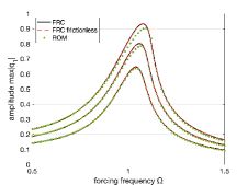
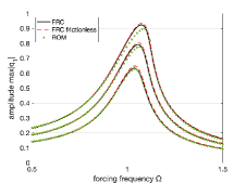
We now compare the SSM-reduced model with the full-order one in terms of forced response curves computed for different forcing amplitudes |𝐟0|subscript𝐟0|\mathbf{f}_{0}| and friction coefficients δ𝛿\delta. For each case, we compute the response of the full system using the numerical continuation software COCO of Dankowicz and Schilder [10] for a range of forcing frequencies. In contrast, results of the reduced model come from the direct integration of the reduced dynamics.
Refer to caption
(a) δ=103𝛿superscript103\delta=10^{-3}
Refer to caption
(b) δ=5103𝛿5superscript103\delta=5\cdot 10^{-3}
Refer to caption
(c) δ=102𝛿superscript102\delta=10^{-2}
Refer to caption
(d) δ=5102𝛿5superscript102\delta=5\cdot 10^{-2}
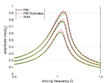
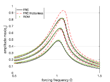
Figure 7: Forced response curves for the forced Shaw-Pierre example with friction, obtained for different values of the friction coefficient δ𝛿\delta. For each case, the amplitudes of the forcing (ϵitalic-ϵ\epsilon in equation (29)) are 0.150.150.15, 0.20.20.2 and 0.250.250.25. The black curves represent the solution of the full-order model; the red dashed curves indicate the forced response without friction; the set of green dots represents the reduced-order model approximation.

Figure 7 shows highly accurate predictions for forced responses for the smallest value of the forcing amplitude ϵitalic-ϵ\epsilon, even for large values of δ𝛿\delta. The prediction error, however, grows for larger forcing amplitudes as we keep the order of approximation for the SSMs cubic. Nevertheless, the reduced order model correctly captures the effect of friction in the system, at least for a range of parameters, as visible especially in Fig. 7d. Indeed, in this case the difference between the system with and without friction is the most evident.

4 Data-driven model reduction of a non-smooth beam model

We now apply our nonsmooth SSM-reduction procedure in a data-driven setting. We consider a finite-element model of a von Kármán beam with clamped-clamped boundary conditions (Jain et al. [19]). Each finite element has three degrees of freedom: axial deformation, transverse displacement and transverse rotation. The beam is approximated by 4 elements, resulting in 9 total degrees of freedom, i.e., an 18-dimensional phase space. The material is aluminium, with Young modulus E=70GPa𝐸70GPaE=70\,\text{GPa}, density ρ=2700Kg/m3𝜌2700superscriptKg/m3\rho=2700\,\text{Kg/}\text{m}^{3}, Poisson ratio ν=0.3𝜈0.3\nu=0.3 and material damping modulus k=1×10⁶Pas𝑘1superscript106Pask=1\times 10^{6}\,\text{Pa}\cdot\text{s}. We set the length 1 [m], the width 5 [cm] and the thickness 2 [cm].

Refer to caption
(a)
Refer to caption
(b)
Refer to caption
(c)
Refer to caption
(d)
Figure 8: LABEL:sub@vkbeam_figure Geometry of the clamped-clamped von Kármán beam. In each of the cases shown in the subplots LABEL:sub@coulomb_friction, LABEL:sub@soft_impact, LABEL:sub@moving_ground, the non-smoothness is localized at the midpoint section A-A, where qmidsubscript𝑞𝑚𝑖𝑑q_{mid} represents the vertical displacement of the beam in that section. LABEL:sub@coulomb_friction: Coulomb friction, LABEL:sub@soft_impact soft impact, LABEL:sub@moving_ground friction on moving ground.

We consider three different cases of non-smoothness introduced at the middle of the beam (section A-A of Fig. 8a), with the parameter δ𝛿\delta playing a different role in each case.

  1. 1.

    Coulomb friction: Dry friction between the node at the middle gives the switching function

    σ(𝐱)=q˙mid,𝜎𝐱subscript˙𝑞𝑚𝑖𝑑\sigma(\mathbf{x})=\dot{q}_{mid}, (31)

    and the switching surface

    Σ±={𝐱N:sign(σ(𝐱))=±1},superscriptΣplus-or-minusconditional-set𝐱superscript𝑁sign𝜎𝐱plus-or-minus1\begin{array}[]{l}\Sigma^{\pm}=\left\{\mathbf{x}\in\mathbb{R}^{N}:\text{sign}(\sigma(\mathbf{x}))=\pm 1\right\},\end{array} (32)

    with N𝑁N denoting the phase space dimension of the discretized beam model. Once discretization has been performed, the equations read

    M𝐪¨+C𝐪˙+K𝐪+𝐟nl(𝐪,𝐪˙)=𝐟δ±,𝑀¨𝐪𝐶˙𝐪𝐾𝐪subscript𝐟𝑛𝑙𝐪˙𝐪superscriptsubscript𝐟𝛿plus-or-minusM\ddot{\mathbf{q}}+C\dot{\mathbf{q}}+K\mathbf{q}+\mathbf{f}_{nl}(\mathbf{q},\dot{\mathbf{q}})=\mathbf{f}_{\delta}^{\pm}, (33)

    where

    𝐟δ±=(0 0,δ, 0 0)T.\mathbf{f}_{\delta}^{\pm}=(0\,\cdot\,\cdot\,\cdot\,0,\,\mp\delta,\,0\,\cdot\,\cdot\,\cdot\,0)^{T}. (34)

    In eq. (34), the forcing acts only on the element located at the midpoint. The behavior within the switching surface is qualitatively the same as in the Shaw-Pierre example of Section 3, in that both crossing and attractive sliding (sticking) regimes are possible. We define a normalized non-smooth coefficient δ~~𝛿\tilde{\delta} by dividing δ𝛿\delta by the maximal elastic force at the midpoint.

  2. 2.

    Soft impact: Impact at the section A-A gives the switching function

    σ(𝐱)=qmid.𝜎𝐱subscript𝑞𝑚𝑖𝑑\sigma(\mathbf{x})=q_{mid}. (35)

    Formally, eq. (33) is still valid, but

    𝐟δ+=𝟎,and𝐟δ=(0 0,δxmid, 0 0)T.\mathbf{f}_{\delta}^{+}=\mathbf{0},\quad\text{and}\quad\mathbf{f}_{\delta}^{-}=(0\,\cdot\,\cdot\,\cdot\,0,\,-\delta x_{mid},\,0\,\cdot\,\cdot\,\cdot\,0)^{T}. (36)

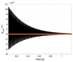
    The behavior of the system is asymmetric with respect to the qmid=0subscript𝑞𝑚𝑖𝑑0q_{mid}=0 position, due to the presence of the further stiffness on one side, as seen in Fig. 9.
    Refer to caption
    Figure 9: Decaying trajectory of the von-Kármán beam with soft-impact located at the midpoint. The orange line refers to the switching between the two sub-regions.

    According to conditions (6) and (7), only crossing between the regions Σ+superscriptΣ\Sigma^{+} and ΣsuperscriptΣ\Sigma^{-} is admissible, while sticking is not allowed. In this case, the coefficient δ𝛿\delta represents the increased stiffness acting on the midpoint of the beam for qmid<0subscript𝑞𝑚𝑖𝑑0q_{mid}<0 and it is naturally normalized by the linear stiffness of the beam.

  3. 3.

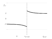
    Friction on moving ground: Assume that the midpoint of the beam rides on a belt moving with constant velocity vgroundsubscript𝑣𝑔𝑟𝑜𝑢𝑛𝑑v_{ground} (Fig. 8d) and dry friction is present between the beam and the belt. The non-smooth forcing term is then given by

    𝐟δ±=(0 0,δfns, 0 0)T,\mathbf{f}_{\delta}^{\pm}=(0\,\cdot\,\cdot\,\cdot\,0,\,\delta f_{ns},\,0\,\cdot\,\cdot\,\cdot\,0)^{\mathrm{T}}, (37)

    where

    fns(q˙mid)=sign(q˙1vground)subscript𝑓𝑛𝑠subscript˙𝑞𝑚𝑖𝑑signsubscript˙𝑞1subscript𝑣𝑔𝑟𝑜𝑢𝑛𝑑\displaystyle f_{ns}(\dot{q}_{mid})=-\text{sign}\,(\dot{q}_{1}-v_{ground}) (38)
    ×(1+αeexp(β|q˙midvground|β)),absent1𝛼𝑒exp𝛽subscript˙𝑞𝑚𝑖𝑑subscript𝑣𝑔𝑟𝑜𝑢𝑛𝑑𝛽\displaystyle\quad\times\left(1+\frac{\alpha}{e}\,\text{exp}\,\left(\frac{\beta-|\dot{q}_{mid}-v_{ground}|}{\beta}\right)\right),

    as shown in Fig. 10. This friction model, similar to that used in Leine and Nijmeijer [22], takes into account that the value of the static friction to be overpowered in order to trigger a relative motion is higher than the kinetic friction force when the relative motion is different from zero.
    Refer to caption
    Figure 10: Friction law dependent on the relative velocity between the midpoint of the von Kármán beam and the moving belt. In contrast to the Coulomb friction model, here the static friction force is different from the dynamic one.

    The switching function in this case is

    σ(𝐱)=q˙midvground,𝜎𝐱subscript˙𝑞𝑚𝑖𝑑subscript𝑣𝑔𝑟𝑜𝑢𝑛𝑑\sigma(\mathbf{x})=\dot{q}_{mid}-v_{ground}, (39)

    which splits the phase space according to the relative motion between the beam element at the midpoint and the moving belt. Interestingly, the difference between static and dynamic friction forces causes the fixed points of the positive and negative systems to be unstable under certain parameter values, triggering a limit cycle. Also in this case both crossing and sticking are allowed: the presence of sticking to the switching surface represents indeed a crucial factor in sustaining the limit cycle.

The data-driven procedure for the computation of the reduced order model is similar for all three piecewise-smooth systems. We constructed two different slow SSMs in each case, one for each region Σ+superscriptΣ\Sigma^{+} and ΣsuperscriptΣ\Sigma^{-}. Within each of these regions, the beam equations are analytic and hence the SSMs are approximated by a convergent Taylor expansion near the respective equilibrium points. We generate decaying trajectories which serve as training data, under 𝐟+superscript𝐟\mathbf{f}^{+} and 𝐟superscript𝐟\mathbf{f}^{-}, separately. The initial condition is a deformed configuration caused by transverse static loading of 12 kN at the midpoint.

We seek a two-dimensional SSM, approximated by a 5th-order expansion and a 5th-order approximation of the reduced dynamics. According to Whitney’s embedding theorem [16], the minimal embedding dimension for a two-dimensional SSM is p=5𝑝5p=5, which is satisfied for our specific case, as we observe the full system. The error of the reconstructed SSM-based reduced model is quantified by the normalized mean-trajectory error (NMTE, see Cenedese et al. [7]) for each region Σ+superscriptΣ\Sigma^{+} and ΣsuperscriptΣ\Sigma^{-}. For a data set of P𝑃P instances of observable points 𝐲jpsubscript𝐲𝑗superscript𝑝\mathbf{y}_{j}\in\mathbb{R}^{p} and their reconstruction 𝐲^jsubscript^𝐲𝑗\mathbf{\hat{y}}_{j}:

NMTE=1𝐲¯1Pj=1P𝐲j𝐲^j,NMTE1norm¯𝐲1𝑃superscriptsubscript𝑗1𝑃normsubscript𝐲𝑗subscript^𝐲𝑗\text{NMTE}=\frac{1}{\|\mathbf{\underline{y}}\|}\frac{1}{P}\sum_{j=1}^{P}\|\mathbf{y}_{j}-\mathbf{\hat{y}}_{j}\|, (40)

where 𝐲¯¯𝐲\mathbf{\underline{y}} is a relevant normalization vector. Finally, we combine the two SSM-based reduced models according to their individual ranges of validity dictated by the switching function. We then employ the model trained on decaying trajectories to predict force response. Based on the arguments of Cenedese et al. [7], moderate forcing terms can simply be added to the reduced model constructed from unforced data.
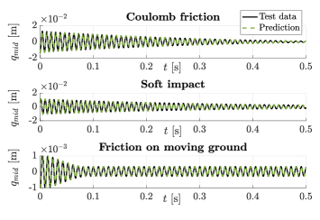
Refer to caption
Figure 11: Model-testing trajectories of the unforced von Kármán beam with different kinds of non-smoothness, and their reconstructions from an unforced, nonsmooth, SSM-based model.

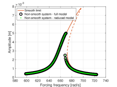
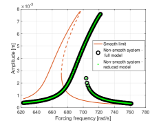
Here, we consider a transversal periodic forcing applied to the midpoint. As seen in Fig. 12 for the Coulomb friction and soft impact cases, the piecewise-smooth reduced order model closely tracks the response for a range of frequencies around the first mode of the system, even when the effect of the non-smoothness factor δ~~𝛿\tilde{\delta} is not negligible. Increasing δ~~𝛿\tilde{\delta} intensifies the dissipation in the system, entailing a lower amplitude of the response. In the soft impact case, δ~~𝛿\tilde{\delta} strengthens the stiffness in some operating region, which leads to an overall shift of the resonance towards higher frequencies.
Refer to caption
(a) Coulomb friction, δ~=1103~𝛿1superscript103\tilde{\delta}=1\cdot 10^{-3}
Refer to caption
(b) soft impact, δ~=5104~𝛿5superscript104\tilde{\delta}=5\cdot 10^{-4}
Figure 12: Response curves for the von Kármán beam forced periodically at the midpoint with Coulomb friction LABEL:sub@VK_coulomb_response and soft impact LABEL:sub@VK_soft_imp_response with the same forcing level (35 kN). In both cases, the effect of non-smoothness is evident. The smooth case (δ~=0~𝛿0\tilde{\delta}=0) and full model cases are computed via the continuation software COCO [10], while the response of the reduced model is retrieved by numerical integration.

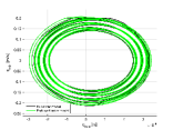
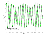
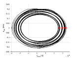
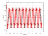
Modeling the sticking regime is delicate, as the constraints confining the trajectory within the switching surface must be enforced. This becomes especially relevant when the dynamics enter and exit the sticking regime multiple times, as in the case of the limit cycle that characterizes the beam with friction on moving ground, for a range of parameters. Since the condition for the sticking regime to occur is expressed in terms of physical variables, choosing the physical coordinates (vertical displacement and velocity at the midpoint) as the reduced variables for the SSM parametrization is advantageous. This is not the standard choice, as we usually employ a pair of coordinates spanning the slowest spectral subspace in order to describe a two-dimensional SSM. More details are given in the B. Let us consider a configuration of parameters wherein the limit cycle is triggered for the autonomous system already: adding forcing in this case generates an invariant periodic or quasiperiodic torus. The behavior of the response depends on the relationship between the frequency of the limit cycle of the autonomous system (fLCsubscript𝑓𝐿𝐶f_{LC}) and that of the forcing term (fFsubscript𝑓𝐹f_{F}). In Fig. 13 we report the case for fF/fLC=1.125subscript𝑓𝐹subscript𝑓𝐿𝐶1.125f_{F}/f_{LC}=1.125, where the reduced order model (in green) is able to accurately capture the multi-frequency periodic solution of the full order system (in black).
Refer to caption
(a)
Refer to caption
(b)
Refer to caption
(c)
Refer to caption
(d)
Figure 13: Periodic orbit lying on a torus generated by external forcing (50N50𝑁50N, fF/fLC=1.125subscript𝑓𝐹subscript𝑓𝐿𝐶1.125f_{F}/f_{LC}=1.125 ) applied to a von Kármán beam with friction on a moving ground, with unstable slowest eigenvalues. Subfigure LABEL:sub@p_map shows the temporal history of the red dots in subfigure LABEL:sub@p_map_phase. Subfigures LABEL:sub@forced_reduced_phase and LABEL:sub@forced_reduced_time_colored compare the reduced-order model (in green) with the full order one (in black).

5 Conclusions

We have presented a nonlinear, SSM-based model reduction procedure applicable to piecewise smooth dynamical systems. Our approach extends the applicability of the spectral submanifolds to a class of problems where non-smoothness plays a significant role in the dynamics of the system. In particular, the classic SSM theory is applied separately to different regions of the phase space where the system is smooth, near hyperbolic fixed points. Proper matching conditions are then enforced as crossing between those regions occurs.

The method proposed here accurately captured the non-smooth dynamics in both equation- and data-driven examples. The equation-driven examples included forced and unforced versions of a 2-DOF nonlinear oscillator with Coulomb friction. In this case, the SSMs involved were computed analytically.

The data-driven examples included forced and unforced von Kármán beam models with different types of non-smooth elements at their midpoints. In this case, the SSMs involved were calculated using an extended version of the SSMLearn algorithm. Not only did the piecewise-smooth reduced order model correctly capture single trajectories for all these different sources of non-smoothness, but it also accurately predicted the forced response. When the sticking regime played a crucial role in the system dynamics (a limit cycle existed for the beam with friction on moving ground), we proposed a specific parametrization of the SSMs based on physical coordinates. We did this to automatically verify the sticking conditions, as they are expressed in those coordinates.

In the present work, we assumed that the phase space is split in two regions, where the system is smooth. We then applied SSM reduction procedure with only one switching surface. In principle, the same procedure can be generalized to multiple switching surfaces, but it would require a careful choice of the reduced physical coordinates for the parametrization of SSMs. Indeed, if one wants to correctly track the sticking regime to different switching surfaces, different relevant physical coordinates might be needed. A further limitation of our method lies in the small value of the normalized non-smoothness parameter, for which the two equilibria, and hence their respective SSMs, lie close to each other.

Possible future work could investigate a more invasive effect of non-smooth elements to the system dynamics. In such a case, the condition relating points across a switching surface we have presented might not be able to furnish a proper initial condition in order for the reduced trajectory to synchronize with the solution of the full system. A new strategy taking into account the dynamics normal to the SSMs may then be required.

Data availability

The data discussed in this work are publicly available at https://github.com/leonardobettini/nonsmoothSSM.

Code availability

The code supporting the results of this work is publicly available at https://github.com/leonardobettini/nonsmoothSSM.

Author contributions

MC and GH designed the research. MC, LB and GH carried out the research. MC and LB developed the software and analyzed the examples. LB wrote the paper. GH lead the research team.

Competing interests

The authors declare no competing interests.

Appendix A Piecewise smooth systems

A.1 Filippov’s closure for piecewise-smooth systems

In order to extend the validity of the governing equations (4) to the switching surface ΣΣ\Sigma, we define an extended system, according to the Filippov’s convex inclusion method

𝐱˙=𝐅(𝐱)={𝐟+(t,𝐱),𝐱Σ+co{𝐟(𝐱),𝐟+(𝐱)}𝐱Σ𝐟(𝐱),𝐱Σ,˙𝐱𝐅𝐱casessuperscript𝐟𝑡𝐱𝐱superscriptΣcosuperscript𝐟𝐱superscript𝐟𝐱𝐱Σsuperscript𝐟𝐱𝐱superscriptΣ\dot{\mathbf{x}}=\mathbf{F}(\mathbf{x})=\begin{cases}\mathbf{f}^{+}(t,\mathbf{x}),&\mathbf{x}\in\Sigma^{+}\\ \text{co}\,\left\{\mathbf{f}^{-}(\mathbf{x}),\mathbf{f}^{+}(\mathbf{x})\right\}&\mathbf{x}\in\Sigma\\ \mathbf{f}^{-}(\mathbf{x}),&\mathbf{x}\in\Sigma^{-}\end{cases}, (41)

where

co{𝐟,𝐟+}={1+λ2𝐟++1λ2𝐟,λ(1,1)},λ=sign(σ(𝐱)).cosuperscript𝐟superscript𝐟1𝜆2superscript𝐟1𝜆2superscript𝐟𝜆11𝜆sign𝜎𝐱\begin{array}[]{l}\displaystyle\text{co}\,\{\mathbf{f}^{-},\mathbf{f}^{+}\}=\left\{\frac{1+\lambda}{2}\mathbf{f}^{+}+\frac{1-\lambda}{2}\mathbf{f}^{-}\,,\lambda\in(-1,1)\right\},\\ \lambda=\text{sign}\,(\sigma(\mathbf{x})).\end{array} (42)

Filippov’s inclusion allows us to derive a model for the dynamics within the switching surface ΣΣ\Sigma. Indeed, exploiting the invariance relationship σ˙(𝐱)=0˙𝜎𝐱0\dot{\sigma}(\mathbf{x})=0, we obtain

λΣ=(𝐟+𝐟+)σ(𝐟𝐟+)σ,superscript𝜆Σsuperscript𝐟superscript𝐟𝜎superscript𝐟superscript𝐟𝜎\lambda^{\Sigma}=\frac{(\mathbf{f}^{-}+\mathbf{f}^{+})\cdot\nabla\sigma}{(\mathbf{f}^{-}-\mathbf{f}^{+})\cdot\nabla\sigma}, (43)
𝐱˙=𝐟Σ=(𝐟σ)𝐟+(𝐟+σ)𝐟(𝐟𝐟+)σ.˙𝐱superscript𝐟Σsuperscript𝐟𝜎superscript𝐟superscript𝐟𝜎superscript𝐟superscript𝐟superscript𝐟𝜎\dot{\mathbf{x}}=\mathbf{f}^{\Sigma}=\frac{(\mathbf{f}^{-}\cdot\nabla\sigma)\mathbf{f}^{+}-(\mathbf{f}^{+}\cdot\nabla\sigma)\mathbf{f}^{-}}{(\mathbf{f}^{-}-\mathbf{f}^{+})\cdot\nabla\sigma}. (44)

A.2 Model reduction strategy

We recall some fundamental concepts about primary smooth SSMs and their relevance for model reduction (Haller and Ponsioen [14]). Restricting ourselves to a single region in which governing equations are smooth, we write

𝐱˙=𝐟(𝐱,𝛀t;ϵ)˙𝐱𝐟𝐱𝛀𝑡italic-ϵ\displaystyle\dot{\mathbf{x}}=\mathbf{f}(\mathbf{x},\mathbf{\Omega}t;\epsilon) =𝐀𝐱+𝐟0+ϵ𝐟1(𝐱,𝛀t),absent𝐀𝐱subscript𝐟0italic-ϵsubscript𝐟1𝐱𝛀𝑡\displaystyle=\mathbf{A}\mathbf{x}+\mathbf{f}_{0}+\epsilon\mathbf{f}_{1}(\mathbf{x},\mathbf{\Omega}t), (45)
𝐟0(𝐱)=𝒪(|𝐱|2),0ϵ1,formulae-sequencesubscript𝐟0𝐱𝒪superscript𝐱20italic-ϵmuch-less-than1\displaystyle\quad\mathbf{f}_{0}(\mathbf{x})=\mathcal{O}(|\mathbf{x}|^{2}),\quad 0\leq\epsilon\ll 1,

where 𝐀n𝐀superscript𝑛\mathbf{A}\in\mathbb{R}^{n} is the constant matrix of the linear part, 𝐟0:nn:subscript𝐟0superscript𝑛superscript𝑛\mathbf{f}_{0}:\mathbb{R}^{n}\to\mathbb{R}^{n} and 𝐟1:n×𝕋ln:subscript𝐟1superscript𝑛superscript𝕋𝑙superscript𝑛\mathbf{f}_{1}:\mathbb{R}^{n}\times\mathbb{T}^{l}\to\mathbb{R}^{n}, where 𝕋l=S1××Slsuperscript𝕋lsuperscript𝑆1superscript𝑆l\mathbb{T}^{\textit{l}}=S^{1}\times...\times S^{\textit{l}} is the l-dimensional torus and with 𝐟0,𝐟1subscript𝐟0subscript𝐟1\mathbf{f}_{0},\mathbf{f}_{1} being class 𝒞rsuperscript𝒞𝑟\mathcal{C}^{r} functions. The degree of smoothness of the right-hand side is r+{,a}𝑟superscript𝑎r\in\mathbb{N}^{+}\cup\{\infty,a\}, where a𝑎a refers to analiticity. The eigenvalues λj=αj+iωjsubscript𝜆𝑗subscript𝛼𝑗𝑖subscript𝜔𝑗\lambda_{j}=\alpha_{j}+i\omega_{j}\in\mathbb{C} of 𝐀𝐀\mathbf{A} are counted with their multiplicites and addressed in descending order according to their real part

ReλnReλn1Reλ1<0.Resubscript𝜆𝑛Resubscript𝜆𝑛1Resubscript𝜆10\text{Re}\lambda_{n}\leq\text{Re}\lambda_{n-1}\leq...\leq\text{Re}\lambda_{1}<0. (46)

The real and imaginary parts of the eigenvectors or generalized eigenvectors of 𝐀𝐀\mathbf{A} relative to the j-th eigenvalue gives rise to the j-th real modal subspace Ejnsubscript𝐸𝑗superscript𝑛E_{j}\subset\mathbb{R}^{n}. The direct sum of modal subspaces defines a spectral subspace

Ej1,,jq=Ej1Ej2Ejq.subscript𝐸subscript𝑗1subscript𝑗𝑞direct-sumsubscript𝐸subscript𝑗1subscript𝐸subscript𝑗2subscript𝐸subscript𝑗𝑞E_{j_{1},...,j_{q}}=E_{j_{1}}\oplus E_{j_{2}}\oplus...\oplus E_{j_{q}}. (47)

If we further assume that Reλj<0jResubscript𝜆𝑗0for-all𝑗\text{Re}\lambda_{j}<0\,\forall j, projecting the linearized system onto the nested hierarchy of slow spectral subspaces

E1E2,Ek:=E1,,kfork=1,,nformulae-sequencesuperscript𝐸1superscript𝐸2assignsuperscript𝐸𝑘subscript𝐸1𝑘for𝑘1𝑛E^{1}\subset E^{2}\subset...,\quad E^{k}:=E_{1,...,k}\,\text{for}\,k=1,...,n (48)

defines a strategy for reducing the order of the linearized dynamics with increasing accuracy as k𝑘k is increased (Galerkin projection method). We want now to study the existence of a nonlinear continuation of such a spectral subspace, in order to be able to reduce the order of the model, but in the presence of nonlinear and also time-dependent terms. In particular, let us fix a specific spectral subspace E=Ej1,,jq𝐸subscript𝐸subscript𝑗1subscript𝑗𝑞E=E_{j_{1},...,j_{q}}. If the non-resonance condition

m,ReλEReλl,λlSpect(A|E),2|m|Σ(E)formulae-sequencesubscript𝑚Re𝜆𝐸Resubscript𝜆𝑙formulae-sequencesubscript𝜆𝑙Spectevaluated-at𝐴𝐸2𝑚Σ𝐸\langle m,\text{Re}\lambda\rangle_{E}\neq\text{Re}\lambda_{l},\quad\lambda_{l}\notin\text{Spect}(A|_{E}),\quad 2\leq|m|\leq\Sigma(E) (49)

holds, then infinitely many nonlinear continuations of E𝐸E exist, for ϵitalic-ϵ\epsilon small enough (Haller et al. [13]). Here |m|:=j=1qmjassign𝑚superscriptsubscript𝑗1𝑞subscript𝑚𝑗|m|:=\sum_{j=1}^{q}m_{j}. In (49), Σ(E)Σ𝐸\Sigma(E) is the absolute spectral quotient defined as

Σ(E)=Int[minλSpect(A)Spect(A|E)ReλmaxλSpect(A|E)Reλ].Σ𝐸Intdelimited-[]subscript𝜆Spect𝐴Spectevaluated-at𝐴𝐸Re𝜆subscript𝜆Spectevaluated-at𝐴𝐸Re𝜆\Sigma(E)=\text{Int}\left[\frac{\displaystyle\min_{\lambda\in\text{Spect}(A)-\text{Spect}(A|_{E})}\text{Re}\lambda}{\displaystyle\max_{\lambda\in\text{Spect}(A|_{E})}\text{Re}\lambda}\right]. (50)

Among all 𝒞Σ(E)+1superscript𝒞Σ𝐸1\mathcal{C}^{\Sigma(E)+1} invariant manifolds there is a unique smoothest one, the primary SSM 𝒲(E)𝒲𝐸\mathcal{W}(E), which can therefore be approximated more accurately than the other infinitely many nonlinear continuations of E𝐸E. In the case of autonomous systems (ϵ=0italic-ϵ0\epsilon=0), the non-resonance condition can be relaxed to

m,λEλl,λlSpect(A|E),2|m|σ(E),formulae-sequencesubscript𝑚𝜆𝐸subscript𝜆𝑙formulae-sequencesubscript𝜆𝑙Spectevaluated-at𝐴𝐸2𝑚𝜎𝐸\langle m,\lambda\rangle_{E}\neq\lambda_{l},\quad\lambda_{l}\notin\text{Spect}(A|_{E}),\quad 2\leq|m|\leq\sigma(E), (51)

where σ(E)𝜎𝐸\sigma(E) is the relative spectral quotient, defined as

σ(E)=Int[minλSpect(A)ReλmaxλSpect(A|E)Reλ].𝜎𝐸Intdelimited-[]subscript𝜆Spect𝐴Re𝜆subscript𝜆Spectevaluated-at𝐴𝐸Re𝜆\sigma(E)=\text{Int}\left[\frac{\displaystyle\min_{\lambda\in\text{Spect}(A)}\text{Re}\lambda}{\displaystyle\max_{\lambda\in\text{Spect}(A|_{E})}\text{Re}\lambda}\right]. (52)

A.3 Equation-driven model reduction for the Shaw-Pierre model

Once we obtain the governing equations of the system centered at the two fixed points 𝐱0±superscriptsubscript𝐱0plus-or-minus\mathbf{x}_{0}^{\pm} (eq. 24), we perform a linear change of coordinates,

𝝃±=𝐕𝜼±,superscript𝝃plus-or-minus𝐕superscript𝜼plus-or-minus\boldsymbol{\xi}^{\pm}=\mathbf{V}\boldsymbol{\eta}^{\pm}, (53)

where

𝜼±=(𝐲±,𝐳±)E1×E2superscript𝜼plus-or-minussuperscript𝐲plus-or-minussuperscript𝐳plus-or-minussubscript𝐸1subscript𝐸2\boldsymbol{\eta}^{\pm}=(\mathbf{y}^{\pm},\mathbf{z}^{\pm})\in E_{1}\times E_{2}

and 𝐕𝐕\mathbf{V} is the matrix composed of the eigenvectors of 𝐀~𝟎subscript~𝐀0\mathbf{\tilde{A}_{0}} as columns. For ease of notation, the superscript ±plus-or-minus\pm is dropped in the following equations. The equations of motion now read

𝐲˙=𝐀~𝐲𝐲+(𝐫𝐟𝐧𝐥𝐈𝐈𝐈)𝐲±(𝐫𝐟𝐧𝐥𝐈𝐈)𝐲=(0.07891.03421.03420.0789)𝐲˙𝐲plus-or-minussubscript~𝐀𝐲𝐲subscript𝐫superscriptsubscript𝐟𝐧𝐥𝐈𝐈𝐈𝐲subscript𝐫superscriptsubscript𝐟𝐧𝐥𝐈𝐈𝐲matrix0.07891.03421.03420.0789𝐲\displaystyle\dot{\mathbf{y}}=\mathbf{\tilde{A}_{y}}\mathbf{y}+\left(\mathbf{r}\,\mathbf{f_{nl}^{III}}\right)_{\mathbf{y}}\pm\left(\mathbf{r}\,\mathbf{f_{nl}^{II}}\right)_{\mathbf{y}}=\begin{pmatrix}-0.0789&1.0342\\ -1.0342&-0.0789\end{pmatrix}\mathbf{y} (54)
+(0.99680.0761)qIII(𝜼)±(0.99680.0761)qII(𝜼)plus-or-minusmatrix0.99680.0761superscript𝑞𝐼𝐼𝐼𝜼matrix0.99680.0761superscript𝑞𝐼𝐼𝜼\displaystyle\quad+\begin{pmatrix}0.9968\\ -0.0761\end{pmatrix}q^{III}(\boldsymbol{\eta})\pm\begin{pmatrix}0.9968\\ -0.0761\end{pmatrix}q^{II}(\boldsymbol{\eta})

and

𝐳˙=𝐀~𝐳𝐳+(𝐫𝐟𝐧𝐥𝐈𝐈𝐈)𝐳±(𝐫𝐟𝐧𝐥𝐈𝐈)𝐳=(0.37111.69871.69870.3711)𝐳˙𝐳plus-or-minussubscript~𝐀𝐳𝐳subscript𝐫superscriptsubscript𝐟𝐧𝐥𝐈𝐈𝐈𝐳subscript𝐫superscriptsubscript𝐟𝐧𝐥𝐈𝐈𝐳matrix0.37111.69871.69870.3711𝐳\displaystyle\dot{\mathbf{z}}=\mathbf{\tilde{A}_{z}}\mathbf{z}+\left(\mathbf{r}\,\mathbf{f_{nl}^{III}}\right)_{\mathbf{z}}\pm\left(\mathbf{r}\,\mathbf{f_{nl}^{II}}\right)_{\mathbf{z}}=\begin{pmatrix}-0.3711&1.6987\\ -1.6987&-0.3711\end{pmatrix}\mathbf{z} (55)
+(0.82780.1808)qIII(𝜼)±(0.82780.1808)qII(𝜼),plus-or-minusmatrix0.82780.1808superscript𝑞𝐼𝐼𝐼𝜼matrix0.82780.1808superscript𝑞𝐼𝐼𝜼\displaystyle\quad+\begin{pmatrix}-0.8278\\ 0.1808\end{pmatrix}q^{III}(\boldsymbol{\eta})\pm\begin{pmatrix}-0.8278\\ 0.1808\end{pmatrix}q^{II}(\boldsymbol{\eta}),

where

qIII(𝜼)=12(0.1645z1+0.3070z2+0.0441y10.4828y2)3superscript𝑞𝐼𝐼𝐼𝜼12superscript0.1645subscript𝑧10.3070subscript𝑧20.0441subscript𝑦10.4828subscript𝑦23q^{III}(\boldsymbol{\eta})=-\frac{1}{2}(0.1645z_{1}+0.3070z_{2}+0.0441y_{1}-0.4828y_{2})^{3}

and

qII(𝜼)=32q0(0.1645z1+0.3070z2+0.0441y10.4828y2)2.superscript𝑞𝐼𝐼𝜼32subscript𝑞0superscript0.1645subscript𝑧10.3070subscript𝑧20.0441subscript𝑦10.4828subscript𝑦22q^{II}(\boldsymbol{\eta})=\frac{3}{2}q_{0}(0.1645z_{1}+0.3070z_{2}+0.0441y_{1}-0.4828y_{2})^{2}.

For each case, we seek a cubic Taylor expansion as an approximation of the slow primary SSM anchored at 𝝃±=0superscript𝝃plus-or-minus0\boldsymbol{\xi}^{\pm}=0 in the form

𝐳=|𝐩|=23𝐡𝐩𝐲𝐩,𝐩=(p1,p2)2,formulae-sequence𝐳superscriptsubscript𝐩23subscript𝐡𝐩superscript𝐲𝐩𝐩subscript𝑝1subscript𝑝2superscript2\mathbf{z}=\sum_{|\mathbf{p}|=2}^{3}\mathbf{h}_{\mathbf{p}}\mathbf{y}^{\mathbf{p}},\qquad\mathbf{p}=(p_{1},p_{2})\in\mathbb{N}^{2}, (56)

where

𝐲𝐩=y1p1y2p2,𝐡𝐩=(h1,𝐩h2,𝐩)2.formulae-sequencesuperscript𝐲𝐩superscriptsubscript𝑦1subscript𝑝1superscriptsubscript𝑦2subscript𝑝2subscript𝐡𝐩matrixsubscript1𝐩subscript2𝐩superscript2\mathbf{y}^{\mathbf{p}}=y_{1}^{p_{1}}\,y_{2}^{p_{2}},\qquad\mathbf{h}_{\mathbf{p}}=\begin{pmatrix}h_{1,\mathbf{p}}\\ h_{2,\mathbf{p}}\end{pmatrix}\in\mathbb{R}^{2}.

The expanded formula is reported in equation (57) below:

{z1±=h1±,(2,0)y12+h1±,(1,1)y1y2+h1±,(0,2)y22+h1±,(3,0)y13+h1±,(2,1)y12y2+h1±,(1,2)y11y22+h1±,(0,3)y23,z2±=h2±,(2,0)y12+h2±,(1,1)y2y2+h2±,(0,2)y22+h2±,(3,0)y13+h2±,(2,1)y12y2+h2±,(1,2)y11y22+h2±,(0,3)y23.casesmissing-subexpressionsuperscriptsubscript𝑧1plus-or-minussuperscriptsubscript1plus-or-minus20superscriptsubscript𝑦12superscriptsubscript1plus-or-minus11subscript𝑦1subscript𝑦2superscriptsubscript1plus-or-minus02superscriptsubscript𝑦22missing-subexpressionsuperscriptsubscript1plus-or-minus30superscriptsubscript𝑦13superscriptsubscript1plus-or-minus21superscriptsubscript𝑦12subscript𝑦2superscriptsubscript1plus-or-minus12superscriptsubscript𝑦11superscriptsubscript𝑦22missing-subexpressionsuperscriptsubscript1plus-or-minus03superscriptsubscript𝑦23missing-subexpressionsuperscriptsubscript𝑧2plus-or-minussuperscriptsubscript2plus-or-minus20superscriptsubscript𝑦12superscriptsubscript2plus-or-minus11subscript𝑦2subscript𝑦2superscriptsubscript2plus-or-minus02superscriptsubscript𝑦22missing-subexpressionsuperscriptsubscript2plus-or-minus30superscriptsubscript𝑦13superscriptsubscript2plus-or-minus21superscriptsubscript𝑦12subscript𝑦2superscriptsubscript2plus-or-minus12superscriptsubscript𝑦11superscriptsubscript𝑦22missing-subexpressionsuperscriptsubscript2plus-or-minus03superscriptsubscript𝑦23otherwise\begin{cases}\begin{aligned} &z_{1}^{\pm}=h_{1}^{\pm,(2,0)}y_{1}^{2}+h_{1}^{\pm,(1,1)}y_{1}y_{2}+h_{1}^{\pm,(0,2)}y_{2}^{2}\\ &\quad+h_{1}^{\pm,(3,0)}y_{1}^{3}+h_{1}^{\pm,(2,1)}y_{1}^{2}y_{2}+h_{1}^{\pm,(1,2)}y_{1}^{1}y_{2}^{2}\\ &\quad+h_{1}^{\pm,(0,3)}y_{2}^{3},\\ &z_{2}^{\pm}=h_{2}^{\pm,(2,0)}y_{1}^{2}+h_{2}^{\pm,(1,1)}y_{2}y_{2}+h_{2}^{\pm,(0,2)}y_{2}^{2}\\ &\quad+h_{2}^{\pm,(3,0)}y_{1}^{3}+h_{2}^{\pm,(2,1)}y_{1}^{2}y_{2}+h_{2}^{\pm,(1,2)}y_{1}^{1}y_{2}^{2}\\ &\quad+h_{2}^{\pm,(0,3)}y_{2}^{3}.\end{aligned}\end{cases} (57)

Also the reduced dynamics can be written in the form of a Taylor expansion:

{r1±=r1±,(1,0)y1+r1±,(0,1)y2+r1±,(2,0)y12+r1±,(1,1)y1y2+r1±,(0,2)y22+r1±,(3,0)y13+r1±,(2,1)y12y2+r1±,(1,2)y11y22+r1±,(0,3)y23r2±=r2±,(1,0)y1+r2±,(0,1)y2+r2±,(2,0)y12+r2±,(1,1)y2y2+r2±,(0,2)y22+r2±,(3,0)y13+r2±,(2,1)y12y2+r2±,(1,2)y11y22+r2±,(0,3)y23.casesmissing-subexpressionsuperscriptsubscript𝑟1plus-or-minussuperscriptsubscript𝑟1plus-or-minus10subscript𝑦1superscriptsubscript𝑟1plus-or-minus01subscript𝑦2superscriptsubscript𝑟1plus-or-minus20superscriptsubscript𝑦12superscriptsubscript𝑟1plus-or-minus11subscript𝑦1subscript𝑦2missing-subexpressionsuperscriptsubscript𝑟1plus-or-minus02superscriptsubscript𝑦22superscriptsubscript𝑟1plus-or-minus30superscriptsubscript𝑦13superscriptsubscript𝑟1plus-or-minus21superscriptsubscript𝑦12subscript𝑦2missing-subexpressionsuperscriptsubscript𝑟1plus-or-minus12superscriptsubscript𝑦11superscriptsubscript𝑦22superscriptsubscript𝑟1plus-or-minus03superscriptsubscript𝑦23missing-subexpressionsuperscriptsubscript𝑟2plus-or-minussuperscriptsubscript𝑟2plus-or-minus10subscript𝑦1superscriptsubscript𝑟2plus-or-minus01subscript𝑦2superscriptsubscript𝑟2plus-or-minus20superscriptsubscript𝑦12superscriptsubscript𝑟2plus-or-minus11subscript𝑦2subscript𝑦2missing-subexpressionsuperscriptsubscript𝑟2plus-or-minus02superscriptsubscript𝑦22superscriptsubscript𝑟2plus-or-minus30superscriptsubscript𝑦13superscriptsubscript𝑟2plus-or-minus21superscriptsubscript𝑦12subscript𝑦2missing-subexpressionsuperscriptsubscript𝑟2plus-or-minus12superscriptsubscript𝑦11superscriptsubscript𝑦22superscriptsubscript𝑟2plus-or-minus03superscriptsubscript𝑦23otherwise\begin{cases}\begin{aligned} &r_{1}^{\pm}=r_{1}^{\pm,(1,0)}y_{1}+r_{1}^{\pm,(0,1)}y_{2}+r_{1}^{\pm,(2,0)}y_{1}^{2}+r_{1}^{\pm,(1,1)}y_{1}y_{2}\\ &\quad+r_{1}^{\pm,(0,2)}y_{2}^{2}+r_{1}^{\pm,(3,0)}y_{1}^{3}+r_{1}^{\pm,(2,1)}y_{1}^{2}y_{2}\\ &\quad+r_{1}^{\pm,(1,2)}y_{1}^{1}y_{2}^{2}+r_{1}^{\pm,(0,3)}y_{2}^{3}\\ &r_{2}^{\pm}=r_{2}^{\pm,(1,0)}y_{1}+r_{2}^{\pm,(0,1)}y_{2}+r_{2}^{\pm,(2,0)}y_{1}^{2}+r_{2}^{\pm,(1,1)}y_{2}y_{2}\\ &\quad+r_{2}^{\pm,(0,2)}y_{2}^{2}+r_{2}^{\pm,(3,0)}y_{1}^{3}+r_{2}^{\pm,(2,1)}y_{1}^{2}y_{2}\\ &\quad+r_{2}^{\pm,(1,2)}y_{1}^{1}y_{2}^{2}+r_{2}^{\pm,(0,3)}y_{2}^{3}.\end{aligned}\end{cases} (58)

The invariance equation on the primary SSM reads

Dy𝐡(𝐲)Ay𝐲+Dy𝐡(𝐲)𝐫y[qIII(𝐲,𝐡(𝐲))±qII(𝐲,𝐡(𝐲))]subscript𝐷𝑦𝐡𝐲subscript𝐴𝑦𝐲subscript𝐷𝑦𝐡𝐲subscript𝐫𝑦delimited-[]plus-or-minussuperscript𝑞𝐼𝐼𝐼𝐲𝐡𝐲superscript𝑞𝐼𝐼𝐲𝐡𝐲\displaystyle D_{y}\mathbf{h}(\mathbf{y})\,A_{y}\,\mathbf{y}+D_{y}\mathbf{h}(\mathbf{y})\,\mathbf{r}_{y}\,\left[q^{III}\left(\mathbf{y},\mathbf{h}(\mathbf{y})\right)\pm q^{II}\left(\mathbf{y},\mathbf{h}(\mathbf{y})\right)\right] (59)
=Az𝐡(𝐲)+𝐫z[qIII(𝐲,𝐡(𝐲))±qII(𝐲,𝐡(𝐲))].absentsubscript𝐴𝑧𝐡𝐲subscript𝐫𝑧delimited-[]plus-or-minussuperscript𝑞𝐼𝐼𝐼𝐲𝐡𝐲superscript𝑞𝐼𝐼𝐲𝐡𝐲\displaystyle\quad=\,A_{z}\,\mathbf{h}(\mathbf{y})+\mathbf{r}_{z}\,\left[q^{III}(\mathbf{y},\mathbf{h}\left(\mathbf{y})\right)\pm q^{II}(\mathbf{y},\mathbf{h}\left(\mathbf{y})\right)\right].

Equating powers of 𝐲𝐲\mathbf{y} leads to a set of linear equations with the parametrization coefficients as unknowns (60 and 61) that can be solved as long as nonresonance conditions are satisfied. The values of the coefficients in (57) and (58) are reported in Tables 2, 4, 6 and 8, for δ=0.1𝛿0.1\delta=0.1.

𝒪(2,0):Dy𝐡(2)Ay𝐲=Az𝐡(2)±𝐫zqII,(2)\displaystyle\mathcal{O}(2,0):\quad D_{y}\mathbf{h}^{(2)}A_{y}\mathbf{y}=A_{z}\mathbf{h}^{(2)}\pm\mathbf{r}_{z}q^{II,(2)} (60)
{a1(2Re(λ1)Re(λ2))a2Im(λ1)b1Im(λ2)=±3αq0rz,1p32a2(2Re(λ1)Re(λ2))+2a1Im(λ1)2a3Im(λ1)b2Im(λ2)=±6αp3p4q0rz,1a3(2Re(λ1)Re(λ2))+a2Im(λ1)b3Im(λ2)=±3αq0rz,1p42b1(2Re(λ1)Re(λ2))+a1Im(λ2)b2Im(λ1)=±3αq0rz,2p32b2(2Re(λ1)Re(λ2))+a2Im(λ2)+2b1Im(λ1)2b3Im(λ1)=±6αp3p4q0rz,2b3(2Re(λ1)Re(λ2))+a3Im(λ2)+b2Im(λ1)=±3αq0rz,2p42casesotherwisesubscript𝑎12Resubscript𝜆1Resubscript𝜆2subscript𝑎2Imsubscript𝜆1subscript𝑏1Imsubscript𝜆2otherwiseabsentplus-or-minus3𝛼subscript𝑞0subscript𝑟𝑧1superscriptsubscript𝑝32otherwisesubscript𝑎22Resubscript𝜆1Resubscript𝜆22subscript𝑎1Imsubscript𝜆12subscript𝑎3Imsubscript𝜆1otherwisesubscript𝑏2Imsubscript𝜆2plus-or-minus6𝛼subscript𝑝3subscript𝑝4subscript𝑞0subscript𝑟𝑧1otherwisesubscript𝑎32Resubscript𝜆1Resubscript𝜆2subscript𝑎2Imsubscript𝜆1subscript𝑏3Imsubscript𝜆2otherwiseabsentplus-or-minus3𝛼subscript𝑞0subscript𝑟𝑧1superscriptsubscript𝑝42otherwisesubscript𝑏12Resubscript𝜆1Resubscript𝜆2subscript𝑎1Imsubscript𝜆2subscript𝑏2Imsubscript𝜆1otherwiseabsentplus-or-minus3𝛼subscript𝑞0subscript𝑟𝑧2superscriptsubscript𝑝32otherwisesubscript𝑏22Resubscript𝜆1Resubscript𝜆2subscript𝑎2Imsubscript𝜆22subscript𝑏1Imsubscript𝜆1otherwise2subscript𝑏3Imsubscript𝜆1plus-or-minus6𝛼subscript𝑝3subscript𝑝4subscript𝑞0subscript𝑟𝑧2otherwisesubscript𝑏32Resubscript𝜆1Resubscript𝜆2subscript𝑎3Imsubscript𝜆2subscript𝑏2Imsubscript𝜆1otherwiseabsentplus-or-minus3𝛼subscript𝑞0subscript𝑟𝑧2superscriptsubscript𝑝42\displaystyle\begin{cases}&a_{1}\left(2\text{Re}(\lambda_{1})-\text{Re}(\lambda_{2})\right)-a_{2}\text{Im}(\lambda_{1})-b_{1}\text{Im}(\lambda_{2})\\ &\quad=\pm 3\alpha q_{0}r_{z,1}p_{3}^{2}\\ &a_{2}\left(2\text{Re}(\lambda_{1})-\text{Re}(\lambda_{2})\right)+2a_{1}\text{Im}(\lambda_{1})-2a_{3}\text{Im}(\lambda_{1})\\ &\quad-b_{2}\text{Im}(\lambda_{2})=\pm 6\alpha p_{3}p_{4}q_{0}r_{z,1}\\ &a_{3}\left(2\text{Re}(\lambda_{1})-\text{Re}(\lambda_{2})\right)+a_{2}\text{Im}(\lambda_{1})-b_{3}\text{Im}(\lambda_{2})\\ &\quad=\pm 3\alpha q_{0}r_{z,1}p_{4}^{2}\\ &b_{1}\left(2\text{Re}(\lambda_{1})-\text{Re}(\lambda_{2})\right)+a_{1}\text{Im}(\lambda_{2})-b_{2}\text{Im}(\lambda_{1})\\ &\quad=\pm 3\alpha q_{0}r_{z,2}p_{3}^{2}\\ &b_{2}\left(2\text{Re}(\lambda_{1})-\text{Re}(\lambda_{2})\right)+a_{2}\text{Im}(\lambda_{2})+2b_{1}\text{Im}(\lambda_{1})\\ &\quad-2b_{3}\text{Im}(\lambda_{1})=\pm 6\alpha p_{3}p_{4}q_{0}r_{z,2}\\ &b_{3}\left(2\text{Re}(\lambda_{1})-\text{Re}(\lambda_{2})\right)+a_{3}\text{Im}(\lambda_{2})+b_{2}\text{Im}(\lambda_{1})\\ &\quad=\pm 3\alpha q_{0}r_{z,2}p_{4}^{2}\\ \end{cases}
𝒪(3,0):Dy𝐡(3)Ay𝐲±Dy𝐡(2)𝐫yqII,(2)=Az𝐡(3)\displaystyle\mathcal{O}(3,0):\quad D_{y}\mathbf{h}^{(3)}A_{y}\mathbf{y}\pm D_{y}\mathbf{h}^{(2)}\mathbf{r}_{y}q^{II,(2)}=A_{z}\mathbf{h}^{(3)} (61)
+𝐫z(qIII,(3)±qII,(3))subscript𝐫𝑧plus-or-minussuperscript𝑞𝐼𝐼𝐼3superscript𝑞𝐼𝐼3\displaystyle\qquad+\mathbf{r}_{z}\left(q^{III,(3)}\pm q^{II,(3)}\right)
{a4(3Re(λ1)Re(λ2))rz,1(6αq0(a1p1+b1p2)p3)a5Im(λ1)b4Im(λ2)±3αp32q0(2a1ry,1+a2ry,2)=rz,1αp33a5(3Re(λ1)Re(λ2))+3a4Im(λ1)2a6Im(λ1)b5Im(λ2)rz,1(3αq0(2p4(a1p1+b1p2)+2p3(a2p1+b2p2)))±3αp32q0(a2ry,1+2a3ry,2)±6αp3p4q0(2a1ry,1+a2ry,2)=rz,13αp32p4a6(3Re(λ1)Re(λ2))+2a5Im(λ1)3a7Im(λ1)b6Im(λ2)rz,1(3αq0(2p4(a2p1+b2p2)+2p3(a3p1+b3p2)))±3αp42q0(2a1ry,1+a2ry,2)±6αp3p4q0(a2ry,1+2a3ry,2)=rz,13αp3p42a7(3Re(λ1)Re(λ2))rz,1(6αq0(a3p1+b3p2)p4)+a6Im(λ1)b7Im(λ2)±3αp42q0(a2ry,1+2a3ry,2)=rz,1αp43b4(3Re(λ1)Re(λ2))rz,2(6αq0(a1p1+b1p2)p3)+a4Im(λ2)b5Im(λ1)±3αp32q0(2b1ry,1+b2ry,2)=rz,2αp33b5(3Re(λ1)Re(λ2))+a5Im(λ2)+3b4Im(λ1)2b6Im(λ1)rz,2(3αq0(2p4(a1p1+b1p2)+2p3(a2p1+b2p2)))±3αp32q0(b2ry,1+2b3ry,2)±6αp3p4q0(2b1ry,1+b2ry,2)=rz,23αp32p4b6(3Re(λ1)Re(λ2))+a6Im(λ2)+2b5Im(λ1)3b7Im(λ1)rz,2(3αq0(2p4(a2p1+b2p2)+2p3(a3p1+b3p2)))±3αp42q0(2b1ry,1+b2ry,2)±6αp3p4q0(b2ry,1+2b3ry,2)=rz,23αp3p42b7(3Re(λ1)Re(λ2))rz,2(6αq0(a3p1+b3p2)p4)+a7Im(λ2)+b6Im(λ1)±3αp42q0(b2ry,1+2b3ry,2)=rz,2αp43\displaystyle\begin{cases}&a_{4}\left(3\text{Re}(\lambda_{1})-\text{Re}(\lambda_{2})\right)\mp r_{z,1}(6\alpha q_{0}(a_{1}p_{1}+b_{1}p_{2})p_{3})\\ &\quad-a_{5}\text{Im}(\lambda_{1})-b_{4}\text{Im}(\lambda_{2})\pm 3\alpha p_{3}^{2}q_{0}(2a_{1}r_{y,1}+a_{2}r_{y,2})\\ &\quad=-r_{z,1}\alpha p_{3}^{3}\\ &a_{5}\left(3\text{Re}(\lambda_{1})-\text{Re}(\lambda_{2})\right)+3a_{4}\text{Im}(\lambda_{1})-2a_{6}\text{Im}(\lambda_{1})\\ &\quad-b_{5}\text{Im}(\lambda_{2})\mp r_{z,1}(3\alpha q_{0}(2p_{4}(a_{1}p_{1}+b_{1}p_{2})\\ &\quad+2p_{3}(a_{2}p_{1}+b_{2}p_{2})))\pm 3\alpha p_{3}^{2}q_{0}(a_{2}r_{y,1}+2a_{3}r_{y,2})\\ &\quad\pm 6\alpha p_{3}p_{4}q_{0}(2a_{1}r_{y,1}+a_{2}r_{y,2})=-r_{z,1}3\alpha p_{3}^{2}p_{4}\\ &a_{6}\left(3\text{Re}(\lambda_{1})-\text{Re}(\lambda_{2})\right)+2a_{5}\text{Im}(\lambda_{1})-3a_{7}\text{Im}(\lambda_{1})\\ &\quad-b_{6}\text{Im}(\lambda_{2})\mp r_{z,1}(3\alpha q_{0}(2p_{4}(a_{2}p_{1}+b_{2}p_{2})\\ &\quad+2p_{3}(a_{3}p_{1}+b_{3}p_{2})))\pm 3\alpha p_{4}^{2}q_{0}(2a_{1}r_{y,1}+a_{2}r_{y,2})\\ &\quad\pm 6\alpha p_{3}p_{4}q_{0}(a_{2}r_{y,1}+2a_{3}r_{y,2})=-r_{z,1}3\alpha p_{3}p_{4}^{2}\\ &a_{7}\left(3\text{Re}(\lambda_{1})-\text{Re}(\lambda_{2})\right)\mp r_{z,1}(6\alpha q_{0}(a_{3}p_{1}+b_{3}p_{2})p_{4})\\ &\quad+a_{6}\text{Im}(\lambda_{1})-b_{7}\text{Im}(\lambda_{2})\pm 3\alpha p_{4}^{2}q_{0}(a_{2}r_{y,1}+2a_{3}r_{y,2})\\ &\quad=-r_{z,1}\alpha p_{4}^{3}\\ &b_{4}\left(3\text{Re}(\lambda_{1})-\text{Re}(\lambda_{2})\right)\mp r_{z,2}(6\alpha q_{0}(a_{1}p_{1}+b_{1}p_{2})p_{3})\\ &\quad+a_{4}\text{Im}(\lambda_{2})-b_{5}\text{Im}(\lambda_{1})\pm 3\alpha p_{3}^{2}q_{0}(2b_{1}r_{y,1}+b_{2}r_{y,2})\\ &\quad=-r_{z,2}\alpha p_{3}^{3}\\ &b_{5}\left(3\text{Re}(\lambda_{1})-\text{Re}(\lambda_{2})\right)+a_{5}\text{Im}(\lambda_{2})+3b_{4}\text{Im}(\lambda_{1})\\ &\quad-2b_{6}\text{Im}(\lambda_{1})\mp r_{z,2}(3\alpha q_{0}(2p_{4}(a_{1}p_{1}+b_{1}p_{2})\\ &\quad+2p_{3}(a_{2}p_{1}+b_{2}p_{2})))\pm 3\alpha p_{3}^{2}q_{0}(b_{2}r_{y,1}+2b_{3}r_{y,2})\\ &\quad\pm 6\alpha p_{3}p_{4}q_{0}(2b_{1}r_{y,1}+b_{2}r_{y,2})=-r_{z,2}3\alpha p_{3}^{2}p_{4}\\ &b_{6}\left(3\text{Re}(\lambda_{1})-\text{Re}(\lambda_{2})\right)+a_{6}\text{Im}(\lambda_{2})+2b_{5}\text{Im}(\lambda_{1})\\ &\quad-3b_{7}\text{Im}(\lambda_{1})\mp r_{z,2}(3\alpha q_{0}(2p_{4}(a_{2}p_{1}+b_{2}p_{2})\\ &\quad+2p_{3}(a_{3}p_{1}+b_{3}p_{2})))\pm 3\alpha p_{4}^{2}q_{0}(2b_{1}r_{y,1}+b_{2}r_{y,2})\\ &\pm 6\alpha p_{3}p_{4}q_{0}(b_{2}r_{y,1}\quad+2b_{3}r_{y,2})=-r_{z,2}3\alpha p_{3}p_{4}^{2}\\ &b_{7}\left(3\text{Re}(\lambda_{1})-\text{Re}(\lambda_{2})\right)\mp r_{z,2}(6\alpha q_{0}(a_{3}p_{1}+b_{3}p_{2})p_{4})\\ &\quad+a_{7}\text{Im}(\lambda_{2})+b_{6}\text{Im}(\lambda_{1})\pm 3\alpha p_{4}^{2}q_{0}(b_{2}r_{y,1}+2b_{3}r_{y,2})\\ &\quad=-r_{z,2}\alpha p_{4}^{3}\par\end{cases}
Table 1: *
(2,0) (1,1) (0,2) (3,0) (2,1) (1,2) (0,3)
h1+superscriptsubscript1h_{1}^{+} 8.2 103superscript10310^{-3} -2.4 102superscript10210^{-2} -7.3 103superscript10310^{-3} 2.7 102superscript10210^{-2} -1.5 103superscript10310^{-3} 2.3 103superscript10310^{-3} -1 103superscript10310^{-3}
h2+superscriptsubscript2h_{2}^{+} 1.5 102superscript10210^{-2} 1.7 102superscript10210^{-2} -2.8 103superscript10310^{-3} 3.4 103superscript10310^{-3} 4.6 102superscript10210^{-2} 7.2 103superscript10310^{-3} 3.2102superscript10210^{-2}

Table 2: Coefficients of the graph-style parametrization for the positive case.
Table 3: *
(2,0) (1,1) (0,2) (3,0) (2,1) (1,2) (0,3)
h1+superscriptsubscript1h_{1}^{+} -8.2 103superscript10310^{-3} 2.4 102superscript10210^{-2} 7.3 103superscript10310^{-3} 2.7 102superscript10210^{-2} -1.5 103superscript10310^{-3} 2.3 103superscript10310^{-3} -1 103superscript10310^{-3}
h2+superscriptsubscript2h_{2}^{+} -1.5 102superscript10210^{-2} -1.7 102superscript10210^{-2} 2.8 103superscript10310^{-3} 3.4 103superscript10310^{-3} 4.6 102superscript10210^{-2} 7.2 103superscript10310^{-3} 3.2 102superscript10210^{-2}

Table 4: Coefficients of the graph-style parametrization for the negative case.
Table 5: *
(1,0) (0,1) (2,0) (1,2) (0,2) (3,0) (2,1) (1,2) (0,3)
r1+superscriptsubscript𝑟1r_{1}^{+} -0.074 1.004 1.4 104superscript10410^{-4} 3.8 103superscript10310^{-3} 2.6 102superscript10210^{-2} -1.8 105superscript10510^{-5} 4.5 104superscript10410^{-4} 1.4 102superscript10210^{-2} 6.5 102superscript10210^{-2}
r2+superscriptsubscript𝑟2r_{2}^{+} -1.004 -0.074 -3.0 105superscript10510^{-5} -8.1 104superscript10410^{-4} -5.5 103superscript10310^{-3} 3.9 106superscript10610^{-6} -9.7 105superscript10510^{-5} -3.1 103superscript10310^{-3} -1.4 102superscript10210^{-2}

Table 6: Coefficients of the reduced dynamics for the positive case.
Table 7: *
(1,0) (0,1) (2,0) (1,2) (0,2) (3,0) (2,1) (1,2) (0,3)
r1+superscriptsubscript𝑟1r_{1}^{+} -0.074 1.004 -1.4 104superscript10410^{-4} -3.8 103superscript10310^{-3} -2.6 102superscript10210^{-2} -1.8 105superscript10510^{-5} 4.5 104superscript10410^{-4} 1.4 102superscript10210^{-2} 6.5 102superscript10210^{-2}
r2+superscriptsubscript𝑟2r_{2}^{+} -1.004 -0.074 3.0 105superscript10510^{-5} 8.1 104superscript10410^{-4} 5.5 103superscript10310^{-3} 3.9 106superscript10610^{-6} -9.7 105superscript10510^{-5} -3.1 103superscript10310^{-3} -1.4 102superscript10210^{-2}

Table 8: Coefficients of the reduced dynamics for the negative case.
Refer to caption
Figure 14: Relative error on the displacement of the first mass for different values of δ𝛿\delta.

A.3.1 Errors

Considering the positive case, we report in Fig. 14 the relative errors between the dynamics of the full system and the reduced one. The initial condition is given slightly outside the SSM: the attracting properties of the SSM are evident as the error reduces significantly with time. Moreover, increasing the value of δ𝛿\delta means intensifying the amplitude of the constant external forcing and therefore the error of the reduced dynamics is shifted upwards.

The invariance error represents the accuracy of the Taylor expansion in approximating the invariant manifold and the reduced dynamics computed on it. It is quantified as

Einv=1Ni=1NLHS(yi)RHS(yi)2RHS(yi)2,subscript𝐸𝑖𝑛𝑣1𝑁superscriptsubscript𝑖1𝑁subscriptnormLHSsubscript𝑦𝑖RHSsubscript𝑦𝑖2subscriptnormRHSsubscript𝑦𝑖2\displaystyle E_{inv}=\frac{1}{N}\sum_{i=1}^{N}\frac{\|\mathrm{LHS}(y_{i})-\mathrm{RHS}(y_{i})\|_{2}}{\|\mathrm{RHS}(y_{i})\|_{2}}, (62)
yiYsD(ρ)={(y1,y2)2:y=ρ},subscript𝑦𝑖subscript𝑌𝑠𝐷𝜌conditional-setsubscript𝑦1subscript𝑦2superscript2norm𝑦𝜌\displaystyle\quad y_{i}\in Y_{s}\subset D(\rho)=\{(y_{1},y_{2})\in\mathbb{R}^{2}:\|y\|=\rho\},

where LHSLHS\mathrm{LHS} and RHSRHS\mathrm{RHS} refer to the left-hand and right-hand sides of equation (59) and ρ𝜌\rho denotes the distance from the fixed point in reduced coordinates (y1,y2)subscript𝑦1subscript𝑦2(y_{1},y_{2}).

Refer to caption
(a)
Refer to caption
(b)
Figure 15: Invariance error for different values of distance from the fixed point 𝐱0+superscriptsubscript𝐱0\mathbf{x}_{0}^{+}.

A.3.2 Choice of initial conditions across SSMs

With reference to Fig. 6, the different methods investigate how enforcing continuity of certain physical variables across the switching surface affects the evolution of the reduced trajectory. The most effective strategy in tracking the full dynamics is the one corresponding to the red line in Fig. 16, where no continuity constraint is enforced.
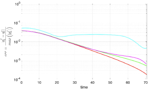
Refer to caption
Figure 16: Relative errors between the solution of the reduced model according to the different strategies and the full model, evaluated for the displacement of the first mass and for δ=103𝛿superscript103\delta=10^{-3}. The colors refer to the strategies depicted in Fig. 6: projection onto the new SSM (red), minimisation of all physical variables (green), continuity of q1subscript𝑞1q_{1} (purple) and continuity of both q1subscript𝑞1q_{1} and q2subscript𝑞2q_{2} (light blue).

A.3.3 Approximation of Poincaré map and invariant set.

The Poincaré map of the full order model introduced in section 3.3 can be approximated by exploiting information from the reduced-order model only. Since the Poincaré map lies close to the intersection between the positive and negative SSMs and the switching surface (blue and red lines in Fig. 17), the invariant set can be approximated by those curves up to specific points, x~edge±subscriptsuperscript~𝑥plus-or-minus𝑒𝑑𝑔𝑒\tilde{x}^{\pm}_{edge}, which need to be estimated and play the same role as xedge±subscriptsuperscript𝑥plus-or-minus𝑒𝑑𝑔𝑒x^{\pm}_{edge} for the full order model. We call the average of the blue and red lines the centerline (dashed line in Fig 17). Recalling that the xedge±superscriptsubscript𝑥𝑒𝑑𝑔𝑒plus-or-minusx_{edge}^{\pm} are the evolution of the closest points to the sticking regime, we want to approximate such configurations for the reduced order model as well. The strategy is described for the computation of x~edgesubscriptsuperscript~𝑥𝑒𝑑𝑔𝑒\tilde{x}^{-}_{edge}, but the same applies to x~edge+subscriptsuperscript~𝑥𝑒𝑑𝑔𝑒\tilde{x}^{+}_{edge}. Referring to Fig. 17, we consider the intersection of the centerline and that of the blue line with the grey surface, representing the configurations on such lines closest to the sticking regime. We take then the average of such intersections to obtain the green circle. Such a point is projected (green cross) onto the negative SSM (not shown in the figure), representing the initial condition sought. The reduced order model is then advected on the negative SSM until the switching surface is hit, identifying x~edgesubscriptsuperscript~𝑥𝑒𝑑𝑔𝑒\tilde{x}^{-}_{edge}. We note that this procedure requires information coming from the reduced order model only.
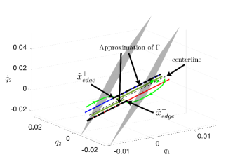
Refer to caption
Figure 17: Approximation of the invariant set induced by the Poincaré map (piecewise continuous green line) exploiting information coming from the reduced order model only.

A.3.4 Non-autonomous problem

The time-dependent SSMs related to the positive and negative cases are sought in the form of a cubic Taylor expansion

𝐳=|𝐩|=23𝐡𝐩𝐲𝐩+ϵ𝐡ϵ(Ωt),𝐩=(p1,p2)2.formulae-sequence𝐳superscriptsubscript𝐩23subscript𝐡𝐩superscript𝐲𝐩italic-ϵsubscript𝐡italic-ϵΩ𝑡𝐩subscript𝑝1subscript𝑝2superscript2\mathbf{z}=\sum_{|\mathbf{p}|=2}^{3}\mathbf{h}_{\mathbf{p}}\mathbf{y}^{\mathbf{p}}+\epsilon\mathbf{h}_{\epsilon}(\Omega t),\qquad\mathbf{p}=(p_{1},p_{2})\in\mathbb{N}^{2}. (63)

The invariance equation is now slightly modified to read

Dy𝐡(𝐲)Ay𝐲+Dy𝐡(𝐲)𝐫y[qIII(𝐲,𝐡(𝐲))±qII(𝐲,𝐡(𝐲))]subscript𝐷𝑦𝐡𝐲subscript𝐴𝑦𝐲subscript𝐷𝑦𝐡𝐲subscript𝐫𝑦delimited-[]plus-or-minussuperscript𝑞𝐼𝐼𝐼𝐲𝐡𝐲superscript𝑞𝐼𝐼𝐲𝐡𝐲\displaystyle D_{y}\mathbf{h}(\mathbf{y})\,A_{y}\,\mathbf{y}+D_{y}\mathbf{h}(\mathbf{y})\,\mathbf{r}_{y}\,\left[q^{III}\left(\mathbf{y},\mathbf{h}(\mathbf{y})\right)\pm q^{II}\left(\mathbf{y},\mathbf{h}(\mathbf{y})\right)\right] (64)
+ϵ(V1𝐟ϵ)y+ϵDt𝐡ϵ=Az𝐡(𝐲)+𝐫z[qIII(𝐲,𝐡(𝐲))\displaystyle\quad+\epsilon\left(V^{-1}\mathbf{f}_{\epsilon}\right)_{y}+\epsilon D_{t}\mathbf{h}_{\epsilon}=\,A_{z}\,\mathbf{h}(\mathbf{y})+\mathbf{r}_{z}\,\Big{[}q^{III}(\mathbf{y},\mathbf{h}\left(\mathbf{y})\right)
±qII(𝐲,𝐡(𝐲))]+ϵ(V1𝐟ϵ)z.\displaystyle\quad\pm q^{II}(\mathbf{y},\mathbf{h}\left(\mathbf{y})\right)\Big{]}+\epsilon\left(V^{-1}\mathbf{f}_{\epsilon}\right)_{z}.

Collecting the terms of order ϵitalic-ϵ\epsilon, we obtain a set of ordinary differential equations, which can be solved by a Fourier representation of the periodic forcing and time dependent terms in the parametrization, whereby the forcing term becomes

𝐡ϵ=n𝐡^ϵ,neinΩt=𝐡^1eiΩt+𝐡^1eiΩt.subscript𝐡italic-ϵsubscript𝑛subscript^𝐡italic-ϵ𝑛superscript𝑒𝑖𝑛Ω𝑡subscript^𝐡1superscript𝑒𝑖Ω𝑡subscript^𝐡1superscript𝑒𝑖Ω𝑡\mathbf{h}_{\epsilon}=\sum_{n}\mathbf{\hat{h}}_{\epsilon,n}e^{in\Omega t}=\mathbf{\hat{h}}_{-1}e^{-i\Omega t}+\mathbf{\hat{h}}_{1}e^{i\Omega t}. (65)

The reduced order model well reproduces the dynamics of the system, as long as the forcing amplitude ϵitalic-ϵ\epsilon remains small and the assumption of small friction coefficient holds. Figure 18 shows how the full trajectory rapidly approaches the reduced one, as the initial condition lies outside the primary SSM. They both eventually land on the attracting limit cycle induced by forcing.
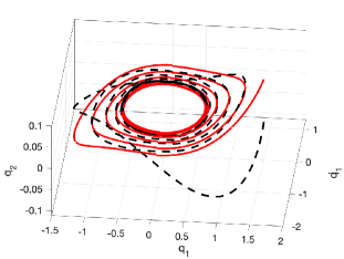
Refer to caption
Figure 18: Trajectories of the full (black dashed) and reduced (red) models in the space (q1,q˙1),q2subscript𝑞1subscript˙𝑞1subscript𝑞2(q_{1},\dot{q}_{1}),q_{2}, starting from the initial condition 𝐱0=(0,0,0.76,0.76)subscript𝐱0000.760.76\mathbf{x}_{0}=(0,0,0.76,0.76), with friction coefficient δ=102𝛿superscript102\delta=10^{-2} and forcing parameter ϵ=101italic-ϵsuperscript101\epsilon=10^{-1}

Appendix B Parametrization of invariant manifolds

In this section, we recall some concepts for the construction of reduced order models with invariant manifolds in a data-driven setting. In particular, referring to [9], we show that one can choose arbitrary reduced coordinates, as long as they describe the invariant manifold as a graph. This justifies the choice of physical coordinates as reduced coordinates in the von Kárman beam example with friction on moving ground, as it allows us to check the sticking condition in a convenient way .
In the setting of eq. (45), we consider a generic spectral subspace

E2q=Ej1Ej2Ejq,superscript𝐸2𝑞direct-sumsubscript𝐸subscript𝑗1subscript𝐸subscript𝑗2subscript𝐸subscript𝑗𝑞E^{2q}=E_{j_{1}}\oplus E_{j_{2}}\oplus...\oplus E_{j_{q}}, (66)

and denote as Spectr(𝐀|E2q)Spectrevaluated-at𝐀superscript𝐸2𝑞\text{Spectr}(\mathbf{A}|_{E^{2q}}) the set of the eigenvalues related to E2qsuperscript𝐸2𝑞E^{2q}. This spectral subspace can be represented by the span of the eigenvectors of 𝐀|E2qevaluated-at𝐀superscript𝐸2𝑞\mathbf{A}|_{E^{2q}}. The eigenvectors are collected as columns of the matrix 𝐕E2q2n×2qsubscript𝐕superscript𝐸2𝑞superscript2𝑛2𝑞\mathbf{V}_{E^{2q}}\in\mathbb{C}^{2n\times 2q} satisfying 𝐀𝐕E2q=𝐕E2q𝐑E2qsubscript𝐀𝐕superscript𝐸2𝑞subscript𝐕superscript𝐸2𝑞subscript𝐑superscript𝐸2𝑞\mathbf{A}\mathbf{V}_{E^{2q}}=\mathbf{V}_{E^{2q}}\mathbf{R}_{E^{2q}}, where 𝐑E2qsubscript𝐑superscript𝐸2𝑞\mathbf{R}_{E^{2q}} is a diagonal matrix containing Spectr(𝐀|E2q)Spectrevaluated-at𝐀superscript𝐸2𝑞\text{Spectr}(\mathbf{A}|_{E^{2q}}) as diagonal. Matrix 𝐕E2qsubscript𝐕superscript𝐸2𝑞\mathbf{V}_{E^{2q}} defines also its adjoint 𝐖E2q2q×2nsubscript𝐖superscript𝐸2𝑞superscript2𝑞2𝑛\mathbf{W}_{E^{2q}}\in\mathbb{C}^{2q\times 2n}, such that 𝐖E2q𝐀=𝐑E2q𝐖E2qsubscript𝐖superscript𝐸2𝑞𝐀subscript𝐑superscript𝐸2𝑞subscript𝐖superscript𝐸2𝑞\mathbf{W}_{E^{2q}}\mathbf{A}=\mathbf{R}_{E^{2q}}\mathbf{W}_{E^{2q}} and normalized according to 𝐖E2q𝐕E2q=𝐈subscript𝐖superscript𝐸2𝑞subscript𝐕superscript𝐸2𝑞𝐈\mathbf{W}_{E^{2q}}\mathbf{V}_{E^{2q}}=\mathbf{I}. Assuming that the spectral subspace E2qsuperscript𝐸2𝑞E^{2q} satisfies the nonresonance conditions (49), then the phase space is characterized by SSMs tangent to E2qsuperscript𝐸2𝑞E^{2q}, among which the primary one is the smoothest and addressed as 𝒲(E2q)𝒲superscript𝐸2𝑞\mathcal{W}(E^{2q}). If we want to study the dynamics on the manifold 𝒲(E2q)𝒲superscript𝐸2𝑞\mathcal{W}(E^{2q}), we need the coordinate chart 𝐲=𝐰(𝐱,𝛀𝐭;ϵ)𝐲𝐰𝐱𝛀𝐭italic-ϵ\mathbf{y}=\mathbf{w}(\mathbf{x},\mathbf{\Omega t};\epsilon) and its inverse, i.e. the parametrization of the manifold 𝐱=𝐯(𝐲,𝛀t;ϵ)𝐱𝐯𝐲𝛀𝑡italic-ϵ\mathbf{x}=\mathbf{v}(\mathbf{y},\mathbf{\Omega}t;\epsilon)

𝐲=𝐰(𝐯(𝐲,𝛀𝐭;ϵ),𝛀𝐭;ϵ),𝐱=𝐯(𝐰(𝐱,𝛀𝐭;ϵ),𝛀𝐭;ϵ).formulae-sequence𝐲𝐰𝐯𝐲𝛀𝐭italic-ϵ𝛀𝐭italic-ϵ𝐱𝐯𝐰𝐱𝛀𝐭italic-ϵ𝛀𝐭italic-ϵ\mathbf{y}=\mathbf{w(\mathbf{v}(\mathbf{y},\mathbf{\Omega}t;\epsilon),\mathbf{\Omega}t;\epsilon)},\quad\mathbf{x}=\mathbf{v(\mathbf{w}(\mathbf{x},\mathbf{\Omega}t;\epsilon),\mathbf{\Omega}t;\epsilon)}. (67)

Hence, the reduced dynamics read

𝐲˙=𝐫(𝐲,𝛀t;ϵ).˙𝐲𝐫𝐲𝛀𝑡italic-ϵ\dot{\mathbf{y}}=\mathbf{r}(\mathbf{y},\mathbf{\Omega}t;\epsilon). (68)

Since the mappings 𝐯,𝐰𝐯𝐰\mathbf{v},\mathbf{w} are invariant under the full and the reduced dynamics 𝐟𝐟\mathbf{f} and 𝐫𝐫\mathbf{r}, we write

{D𝐲𝐯(𝐲,𝛀t;ϵ)𝐫(𝐲,𝛀t;ϵ)+Dt𝐯(𝐲,𝛀t;ϵ)=𝐟(𝐯(𝐲,𝛀t;ϵ),𝛀t;ϵ),D𝐱𝐰(𝐱,𝛀t;ϵ)𝐟(𝐱,𝛀t;ϵ)+Dt𝐰(𝐱,𝛀t;ϵ)=𝐫(𝐰(𝐱,𝛀t;ϵ),𝛀t;ϵ).casesmissing-subexpressionsubscript𝐷𝐲𝐯𝐲𝛀𝑡italic-ϵ𝐫𝐲𝛀𝑡italic-ϵsubscript𝐷𝑡𝐯𝐲𝛀𝑡italic-ϵmissing-subexpressionabsent𝐟𝐯𝐲𝛀𝑡italic-ϵ𝛀𝑡italic-ϵmissing-subexpressionsubscript𝐷𝐱𝐰𝐱𝛀𝑡italic-ϵ𝐟𝐱𝛀𝑡italic-ϵsubscript𝐷𝑡𝐰𝐱𝛀𝑡italic-ϵmissing-subexpressionabsent𝐫𝐰𝐱𝛀𝑡italic-ϵ𝛀𝑡italic-ϵotherwise\begin{cases}\begin{aligned} &D_{\mathbf{y}}\mathbf{v}(\mathbf{y},\mathbf{\Omega}t;\epsilon)\,\mathbf{r}(\mathbf{y},\mathbf{\Omega}t;\epsilon)+D_{t}\mathbf{v}(\mathbf{y},\mathbf{\Omega}t;\epsilon)\\ &\quad=\mathbf{f}(\mathbf{v}(\mathbf{y},\mathbf{\Omega}t;\epsilon),\mathbf{\Omega}t;\epsilon),\\ &D_{\mathbf{x}}\mathbf{w}(\mathbf{x},\mathbf{\Omega}t;\epsilon)\,\mathbf{f}(\mathbf{x},\mathbf{\Omega}t;\epsilon)+D_{t}\mathbf{w}(\mathbf{x},\mathbf{\Omega}t;\epsilon)\\ &\quad=\mathbf{r}(\mathbf{w}(\mathbf{x},\mathbf{\Omega}t;\epsilon),\mathbf{\Omega}t;\epsilon).\end{aligned}\end{cases} (69)

Moreover, as the SSM depends smoothly on the parameter ϵitalic-ϵ\epsilon, we seek the expansions for 𝐰,𝐯𝐰𝐯\mathbf{w},\mathbf{v} and 𝐫𝐫\mathbf{r} in the form

{𝐰(𝐱,𝛀t;ϵ)=𝐖0+𝐰nl(𝐱)+ϵ𝐰1(𝛀t)+𝒪(ϵ𝐱),𝐯(𝐲,𝛀t;ϵ)=𝐕0+𝐯nl(𝐲)+ϵ𝐯1(𝛀t)+𝒪(ϵ𝐲),𝐫(𝐲,𝛀t;ϵ)=𝐑0+𝐫nl(𝐲)+ϵ𝐫1(𝛀t)+𝒪(ϵ𝐲),cases𝐰𝐱𝛀𝑡italic-ϵsubscript𝐖0subscript𝐰𝑛𝑙𝐱italic-ϵsubscript𝐰1𝛀𝑡𝒪italic-ϵnorm𝐱otherwise𝐯𝐲𝛀𝑡italic-ϵsubscript𝐕0subscript𝐯𝑛𝑙𝐲italic-ϵsubscript𝐯1𝛀𝑡𝒪italic-ϵnorm𝐲otherwise𝐫𝐲𝛀𝑡italic-ϵsubscript𝐑0subscript𝐫𝑛𝑙𝐲italic-ϵsubscript𝐫1𝛀𝑡𝒪italic-ϵnorm𝐲otherwise\begin{cases}\mathbf{w}(\mathbf{x},\mathbf{\Omega}t;\epsilon)=\mathbf{W}_{0}+\mathbf{w}_{nl}(\mathbf{x})+\epsilon\mathbf{w}_{1}(\mathbf{\Omega}t)+\mathcal{O}(\epsilon\|\mathbf{x}\|),\\ \mathbf{v}(\mathbf{y},\mathbf{\Omega}t;\epsilon)=\mathbf{V}_{0}+\mathbf{v}_{nl}(\mathbf{y})+\epsilon\mathbf{v}_{1}(\mathbf{\Omega}t)+\mathcal{O}(\epsilon\|\mathbf{y}\|),\\ \mathbf{r}(\mathbf{y},\mathbf{\Omega}t;\epsilon)=\mathbf{R}_{0}+\mathbf{r}_{nl}(\mathbf{y})+\epsilon\mathbf{r}_{1}(\mathbf{\Omega}t)+\mathcal{O}(\epsilon\|\mathbf{y}\|),\\ \end{cases} (70)

with 𝐖02q×2nsubscript𝐖0superscript2𝑞2𝑛\mathbf{W}_{0}\in\mathbb{C}^{2q\times 2n}, 𝐕02n×2qsubscript𝐕0superscript2𝑛2𝑞\mathbf{V}_{0}\in\mathbb{C}^{2n\times 2q} and 𝐑02q×2qsubscript𝐑0superscript2𝑞2𝑞\mathbf{R}_{0}\in\mathbb{C}^{2q\times 2q} and such that range(𝐕0)=E2qrangesubscript𝐕0superscript𝐸2𝑞\text{range}(\mathbf{V}_{0})=E^{2q} and Spectr(𝐑0)=Spectr(𝐀|E2q)Spectrsubscript𝐑0Spectrevaluated-at𝐀superscript𝐸2𝑞\text{Spectr}(\mathbf{R}_{0})=\text{Spectr}(\mathbf{A}|_{E^{2q}}). Substituting the expansions (70) into (67) and taking the linear contributions for ϵ=0italic-ϵ0\epsilon=0, we obtain

𝐖0𝐕0=𝐈,subscript𝐖0subscript𝐕0𝐈\mathbf{W}_{0}\mathbf{V}_{0}=\mathbf{I}, (71)

while considering equations (69) gives:

𝐖0𝐀𝐕0=𝐑0.subscript𝐖0subscript𝐀𝐕0subscript𝐑0\mathbf{W}_{0}\mathbf{A}\mathbf{V}_{0}=\mathbf{R}_{0}. (72)

Since the spectra of 𝐑0subscript𝐑0\mathbf{R}_{0} and that of 𝐀𝐀\mathbf{A} are the same,

𝐑0=𝐏𝐑E2q𝐏1,subscript𝐑0subscript𝐏𝐑superscript𝐸2𝑞superscript𝐏1\mathbf{R}_{0}=\mathbf{P}\mathbf{R}_{E^{2q}}\mathbf{P}^{-1}, (73)

holds, which, coupled with equation (72), yields:

𝐖0=𝐏𝐖E2qand𝐕0=𝐕E2q𝐏1.formulae-sequencesubscript𝐖0subscript𝐏𝐖superscript𝐸2𝑞andsubscript𝐕0subscript𝐕superscript𝐸2𝑞superscript𝐏1\mathbf{W}_{0}=\mathbf{P}\mathbf{W}_{E^{2q}}\quad\text{and}\quad\mathbf{V}_{0}=\mathbf{V}_{E^{2q}}\mathbf{P}^{-1}. (74)

In principle, the coordinate chart can be arbitrarily chosen as a projection to the reduced coordinates defined by 𝐖0subscript𝐖0\mathbf{W}_{0}, as long as it is able to describe the manifold as a graph. In other words, once we define 𝐖0subscript𝐖0\mathbf{W}_{0} and we know the eigenvectors spanning the tangent plane to the manifold VE2qsubscript𝑉superscript𝐸2𝑞V_{E^{2q}}, then from (71) and the second relation of (74) we compute the matrix 𝐏𝐏\mathbf{P} as

𝐏=𝐖0𝐕E2q.𝐏subscript𝐖0subscript𝐕superscript𝐸2𝑞\mathbf{P}=\mathbf{W}_{0}\mathbf{V}_{E^{2q}}. (75)

This means that the vectors spanning the plane where the new reduced coordinates live (columns of 𝐕0subscript𝐕0\mathbf{V}_{0}) define an alternative coordinate chart of the same manifold, as long as the matrix 𝐏𝐏\mathbf{P} is nonsingular. When we add forcing (ϵ0italic-ϵ0\epsilon\neq 0), we need to solve

𝐫1(𝛀t)=𝐖0𝐀𝐯1(𝛀t)+𝐖0𝐟1(𝟎,𝛀t;0),subscript𝐫1𝛀𝑡subscript𝐖0subscript𝐀𝐯1𝛀𝑡subscript𝐖0subscript𝐟10𝛀𝑡0\displaystyle\mathbf{r}_{1}(\boldsymbol{\Omega}t)=\mathbf{W}_{0}\mathbf{A}\mathbf{v}_{1}(\boldsymbol{\Omega}t)+\mathbf{W}_{0}\mathbf{f}_{1}\left(\mathbf{0},\boldsymbol{\Omega}t;0\right), (76)
𝐯1(𝛀t)=(𝐈𝐕0𝐖0)𝐀𝐯1(𝛀t)subscript𝐯1𝛀𝑡𝐈subscript𝐕0subscript𝐖0subscript𝐀𝐯1𝛀𝑡\displaystyle\mathbf{v}_{1}(\boldsymbol{\Omega}t)=\left(\mathbf{I}-\mathbf{V}_{0}\mathbf{W}_{0}\right)\mathbf{A}\mathbf{v}_{1}(\boldsymbol{\Omega}t)
+(𝐈𝐕0𝐖0)𝐟1(𝟎,𝛀t;0).𝐈subscript𝐕0subscript𝐖0subscript𝐟10𝛀𝑡0\displaystyle\qquad+\left(\mathbf{I}-\mathbf{V}_{0}\mathbf{W}_{0}\right)\mathbf{f}_{1}\left(\mathbf{0},\boldsymbol{\Omega}t;0\right).

which takes into account additional non-modal contributions to the forcing in reduced coordinates, as explained in Cenedese et al. [9].

References

  • Axås et al. [2023] Axås, J., Cenedese, M., Haller, G., 2023. Fast data-driven model reduction for nonlinear dynamical systems. Nonlinear Dyn. 111, 7941–7957.
  • Benner et al. [2015] Benner, P., Gugercin, S., Willcox, K., 2015. A survey of projection-based model reduction methods for parametric dynamical systems. SIAM Review 57, 483–531.
  • Brunton et al. [2020] Brunton, S.L., Noack, B.R., Koumoutsakos, P., 2020. Machine learning for fluid mechanics. Annu. Rev. Fluid Mech. 52, 477–508.
  • Cabré et al. [2003] Cabré, X., Fontich, E., de la Llave, R., 2003. The parameterization method for invariant manifolds i: manifolds associated to non-resonant subspaces. Indiana Univ. Math. J. , 283–328.
  • Cardin et al. [2013] Cardin, P.T., Da Silva, P.R., Teixeira, M.A., 2013. On singularly perturbed Filippov systems. Eur. J. Appl. Math. 24, 835–856.
  • Cardin et al. [2015] Cardin, P.T., de Moraes, J.R., da Silva, P.R., 2015. Persistence of periodic orbits with sliding or sewing by singular perturbation. J. Math. Anal. Appl. 423, 1166–1182.
  • Cenedese et al. [2022] Cenedese, M., Axås, J., Bäuerlein, B., Avila, K., Haller, G., 2022. Data-driven modeling and prediction of non-linearizable dynamics via spectral submanifolds. Nat. Commun. 13, 872.
  • Cenedese et al. [2021] Cenedese, M., Axås, J., Yang, H., Eriten, M., Haller, G., 2021. Data-driven Nonlinear Model Reduction to Spectral Submanifolds in Mechanical Systems. Phil. Trans. R. Soc. A. 380.
  • Cenedese et al. [2023] Cenedese, M., Jain, S., Marconi, J., Haller, G., 2023. Data-Assisted Non-Intrusive Model Reduction for Forced Nonlinear Finite Elements Models. arXiv:2311.17865 .
  • Dankowicz and Schilder [2013] Dankowicz, H., Schilder, F., 2013. Recipes for Continuation. Society for Industrial and Applied Mathematics, Philadelphia, PA.
  • Filippov [1988] Filippov, A.F., 1988. Differential equations with discontinuous righthand sides. volume 18 of Mathematics and its Applications (Soviet Series). Kluwer Academic Publishers Group, Dordrecht.
  • Ghadami and Epureanu [2022] Ghadami, A., Epureanu, B.I., 2022. Data-driven prediction in dynamical systems: recent developments. Philos. Trans. Royal Soc. A. 380, 20210213.
  • Haller et al. [2023] Haller, G., Kaszás, B., Liu, A., Axås, J., 2023. Nonlinear model reduction to fractional and mixed-mode spectral submanifolds. Chaos 33.
  • Haller and Ponsioen [2016] Haller, G., Ponsioen, S., 2016. Nonlinear normal modes and spectral submanifolds: Existence, uniqueness and use in model reduction. Nonlinear Dyn. 86.
  • Haro and de la Llave [2006] Haro, A., de la Llave, R., 2006. A parameterization method for the computation of invariant tori and their whiskers in quasi-periodic maps: rigorous results. J. Differ. Equ. 228, 530–579.
  • Hassler Whitney [1944] Hassler Whitney, 1944. The Self-Intersections of a Smooth n-Manifold in 2n-Space. Ann. Math. 45, 220–246.
  • Jain and Haller [2022] Jain, S., Haller, G., 2022. How to compute invariant manifolds and their reduced dynamics in high-dimensional finite element models. Nonlinear Dyn. 107, 1–34.
  • Jain et al. [2023] Jain, S., Li, M., Thurnher, T., Haller, G., 2023. SSMTool: Computation of invariant manifolds in high-dimensional mechanics problems.
  • Jain et al. [2017] Jain, S., Tiso, P., Haller, G., 2017. Exact Nonlinear Model Reduction for a von Karman beam: Slow-Fast Decomposition and Spectral Submanifolds. J. Sound Vib. 423.
  • Kaszás et al. [2022] Kaszás, B., Cenedese, M., Haller, G., 2022. Dynamics-based machine learning of transitions in Couette flow. Phys. Rev. Fluids 7.
  • Küpper [2008] Küpper, T., 2008. Invariant cones for non-smooth dynamical systems. Math. Comput. Simul. 79, 1396–1408.
  • Leine and Nijmeijer [2004] Leine, R., Nijmeijer, H., 2004. Dynamics and Bifurcations of Non-Smooth Mechanical Systems. volume 18.
  • Li and Haller [2022] Li, M., Haller, G., 2022. Nonlinear analysis of forced mechanical systems with internal resonance using spectral submanifolds, Part II: Bifurcation and quasi-periodic response. Nonlinear Dyn. 110, 1045–1080.
  • Li et al. [2022] Li, M., Jain, S., Haller, G., 2022. Nonlinear analysis of forced mechanical systemswith internal resonance using spectral submanifolds, Part I: Periodic response and forced response curve. Nonlinear Dyn. 110, 1005–1043.
  • Mikhlin and Avramov [2023] Mikhlin, Y., Avramov, K.V., 2023. Nonlinear normal modes of vibrating mechanical systems: 10 years of progress. Appl. Mech. Rev. , 1–57.
  • Ponsioen et al. [2020] Ponsioen, S., Jain, S., Haller, G., 2020. Model reduction to spectral submanifolds and forced-response calculation in high-dimensional mechanical systems. J. Sound Vib. 488, 115640.
  • Rowley and Dawson [2017] Rowley, C.W., Dawson, S.T., 2017. Model reduction for flow analysis and control. Annu. Rev. Fluid Mech. 49, 387–417.
  • Shaw and Pierre [1993] Shaw, S., Pierre, C., 1993. Normal modes for non-linear vibratory systems. J. Sound Vib. 164, 85–124.
  • Shaw and Pierre [1994] Shaw, S., Pierre, C., 1994. Normal modes of vibration for non-linear continuous systems. J. Sound Vib. 169, 319–347.
  • Shaw et al. [1999] Shaw, S.W., Pierre, C., Pesheck, E., 1999. Modal analysis-based reduced-order models for nonlinear structures : An invariant manifold approach. Shock Vib. Dig. 31, 3–16.
  • Szalai [2019] Szalai, R., 2019. Model Reduction of Non-densely Defined Piecewise-Smooth Systems in Banach Spaces. J. Nonlinear Sci. 29.
  • Taira et al. [2017] Taira, K., Brunton, S.L., Dawson, S.T., Rowley, C.W., Colonius, T., McKeon, B.J., Schmidt, O.T., Gordeyev, S., Theofilis, V., Ukeiley, L.S., 2017. Modal analysis of fluid flows: An overview. AIAA J. 55, 4013–4041.
  • Touzé et al. [2021] Touzé, C., Vizzaccaro, A., Thomas, O., 2021. Model order reduction methods for geometrically nonlinear structures: a review of nonlinear techniques. Nonlinear Dyn. 105, 1141–1190.
  • Weiss et al. [2012] Weiss, D., Küpper, T., Hosham, H., 2012. Invariant manifolds for nonsmooth systems. Phys. D: Nonlinear Phenom. 241, 1895–1902.
  • Weiss et al. [2015] Weiss, D., Küpper, T., Hosham, H., 2015. Invariant manifolds for nonsmooth systems with sliding mode. Math. Comput. Simul. 110, 15–32.