Training Convolutional Neural Networks with the Forward-Forward Algorithm

Abstract

The recent successes in analyzing images with deep neural networks are almost exclusively achieved with Convolutional Neural Networks (CNNs). The training of these CNNs, and in fact of all deep neural network architectures, uses the backpropagation algorithm, where the output of the network is compared with the desired result, and the difference is then used to tune the weights of the network towards the desired outcome. In a 2022 preprint, Geoffrey Hinton suggested an alternative way of training which passes the desired results together with the images at the input of the network. This so called Forward-Forward (FF) algorithm has up to now only been used in fully connected networks. In this paper, we show how the FF paradigm can be extended to CNNs. Our FF-trained CNN, featuring a novel spatially-extended labeling technique, achieves a classification accuracy of 99.16% on the MNIST hand-written digits data set. We show how different hyperparameters affect the performance of the proposed algorithm and compare the results with CNNs trained with the standard backpropagation approach. Furthermore, we demonstrate that Class Activation Maps can be used to investigate which type of features are learnt by the FF algorithm.

Keywords: forward-forward, backpropagation, convolutional neural networks, class activation maps, MNIST classification.

1 Introduction

Machine learning using deep neural networks (DNN) continues to transform human life in areas as different as art (DALL-E, stable diffusion), medicine (Alpha-Fold), transport (self-driving cars, any time now), or information retrieval (ChatGPT, Bard). Here, the adjective deep refers to the number of layers of artificial neurons, which can go up to the hundreds. Training these networks means shifting the weights connecting the layers from their initial, random values to values which produce the correct predictions at the output layer of the DNN. This is achieved with the help of a loss function that computes the aggregate difference between the predicted output and the accurate results, which must be known for the training examples. The algorithm behind the training is some variant of gradient descent: in each round of training each weight is shifted a bit into the direction minimizing the loss by using the derivative of the loss function with respect to that weight. Taking the derivative of a loss function with respect to a given weight is straightforward for a single, output layer. Training the weights of the earlier layers in DNNs requires the gradient computation to be performed iteratively by applying the chain rule (Rumelhart et al., 1986). This process is called backpropagation (BP). Due to its importance, the term BP is also often used loosely to refer to the entire learning algorithm including the gradient descent.

Backpropagation, respectively multi-layer gradient descent, has a number of downsides: first, it requires the storage of intermediate results. Depending on the optimizer, the memory consumption of BP is up to 5 times larger than the requirement for storing the weights alone (Hugging Face Community, 2023). This becomes a problem when training large models on GPU cards with limited memory. Second, under the name neuromorphic computing, there is an ongoing search of hardware alternatives to CMOS semiconductors, driven by the desire to decrease power consumption and increase processing speed (Christensen et al., 2022). On these new hardware platforms, it is often impossible to implement an analog of BP, raising the need for alternative training algorithm. Finally, evolution has clearly developed learning algorithms for neural networks such as our brain. However, those algorithms seem to be quite (but maybe not completely, see e.g. Lillicrap et al., 2020) different from BP. Given the in general high performance of evolutionary solutions to problems, this raises the question if deep learning could also gain from biologically plausible alternatives to BP.

Due to these limitations, there is an ongoing search for alternative training methods. The most radical approach is to abandon the loss function completely and use a new learning paradigm. Neural networks trained with variants of the locally acting Hebbian learning rule (neurons that fire together wire together) have been shown to be competitive with BP (Journé et al., 2023; Zhou, 2022). Another approach, Equilibrium Propagation (Scellier and Bengio, 2017) is a learning framework for energy based models with symmetric connections between neurons. Layer-wise Feedback Propagation (Weber et al., 2023) removes the need for a gradient computation by replacing the objective of reducing the loss with computing a reward signal from the network output, and propagating that signal backward into the net. In contrast, the most conservative approach is to keep gradient descent, but to replace the required gradients with an estimate computed from the difference in loss of two forward passes with slightly modified weights. While the naive version of this approach, labeled zeroth order optimization, can be expected to be extremely inefficient, modern variants seem to be competitive (Baydin et al., 2022; McCaughan et al., 2023; Malladi et al., 2023; zhao:23PINN).

A third category of algorithms maintains the idea to update the weights using derivatives of some signal, which involves the difference between the present state of the network and the target state. But it relaxes the requirement to backpropagate that signal from the output layer towards the earlier layers. This can either be done by using exclusively an output-derived error signal for training each intermediate layer (Nøkland, 2016; Flügel et al., 2023), or by training each layer with locally available information gathered in two consecutive forward passes. An example of the latter is the ”Present the Error to Perturb the Input To modulate Activity technique” (PEPITA), which performs the second forward pass with the sum of the input signal used in the first pass and some random projection of the error signal from that pass (Dellaferrera and Kreiman, 2022; Farinha et al., 2023).

Another example of the use of local information gathered in consecutive runs to update the weights is the Forward-Forward (FF) algorithm (Hinton (2022)) proposed by Geoffrey Hinton in December 2022. FF training combines two ideas. First, the weights of a given layer are updated using gradients of a locally defined goodness function, which in Hinton (2022) is taken to be the sum of the squares of the activities in that layer. Second, the labels are included in the training data, which allows the neurons to learn them together. In order to understand which features of the data vote for a given label, half of the data set is comprised of labels combined with wrong images. For this negative data the weights are changed in order to minimize the goodness. In contrast, for the correctly labeled, positive data the weights are modified to maximize the goodness. Both these objectives can be achieved with a local gradient descent, with no need for BP. The term Forward-Forward now refers to having two subsequent training steps, one with positive and one with negative data.

When generalizing this training method to multi-layer networks, it is important to assure that each subsequent layer needs to do more than just measure the length of the activity vector of the previous one. This is achieved by using layer normalization (Ba et al., 2016) which normalizes the activity vector for each sample. This is best summarized by the description in Hinton (2022): the activity vector in the first hidden layer has a length and an orientation. The length is used to define the goodness for that layer and only the orientation is passed to the next layer. There are two ways of using a FF trained network for inference. First, we can simultaneously train a linear classifier using the activities of the neurons in the different layers as input. Alternatively, we can create multiple copies of the data set under consideration and combine each copy with one of the possible labels. The correct label is then the one with the largest goodness during its forward pass. Note that this approach multiplies the amount of computation required for inference with a factor equal to the number of labels.

Given the repute of the proposer, it is not surprising that the Forward-Forward algorithm has inspired a number of groups to suggest modified and adapted versions. Examples include the combination with a generative model (Ororbia and Mali, 2023), multiple convolutional blocks (not trained with FF) (zhao:23ForwardAlgo), or extending FF training to graph neural networks (Paliotta et al., 2023) and spiking neural networks (Ororbia, 2023). In accordance with the neuromorphic computation motivation of moving beyond BP, the FF algorithm has also been used to train optical neural networks (Oguz et al., 2023) and microcontroller units with low computational resources (De Vita et al., 2023). Another line of research tries to improve FF by modifying how the goodness is computed (Lee and Song, 2023; Lorberbom et al., 2023; Gandhi et al., 2023), by understanding the sparsity of activation in FF trained networks (Tosato et al., 2023; Yang, 2023), or by exploring the capabilities of FF for self-supervised learning (Brenig and Timofte, 2023). There has been less activity in terms of practical applications of the FF algorithm. Particularly, in the classification of real world images it has been noted that FF performs worse than BP (Reyes-Angulo and Paheding, 2023) or has to be combined with BP to achieve satisfying results (Paheding and Reyes-Angulo, 2023). We propose that this lack of applications is due to the absence of a method to train the mainstay of modern image processing, Convolutional Neural Networks (CNN) (Rawat and Wang, 2017), with the FF algorithm. The ideas presented here close this gap.

This paper is structured as following: in Section 2 we will first introduce our spatial-extended labeling technique, which is crucial to preserve the label information during convolution. Then we will discuss the details of our implementation of the FF-based learning and inference. The results in Section 3 start with a discussion of the optimal results we obtained on the MNIST hand written digits classification. In Section 3.2, we describe our search for the optimal hyperparameters (using validation data). Section 3.3 shows how Class Activation Maps (CAMs) can be used to get a better understanding of the features learned during training. We close in Section 4 with a short discussion.

2 Materials and methods

This section will first discuss our new technique for labeling the positive and negative data sets, before explaining our implementation of the FF algorithm in detail.

2.1 Spatially-extended labeling

Fully connected DNNs establish connections between each pixel within an image and with each neuron in the next layer. The size of images is often of the order of mega pixels and typical layers have hundreds of neurons. This results in a number of weights to be trained which far exceeds the information available in typical training data sets. In contrast, convolutional layers use small filter kernels, typically sized in the range of 3 by 3 to 7 by 7 pixels, which are applied to all possible positions of the much larger input picture. In this way, each filter creates a new, processed version of the input image. Because the training algorithm only needs to learn the weights in these filter kernels, it is possible to apply hundreds of these kernels in parallel and still have order of magnitudes less parameters to train than in a fully connected network.

FF training requires the labels to be added to the input images. Hinton (2022) achieves this with an one-hot encoding, in which the label information is confined to the first 10 pixels in the upper left region of each image. Figure 1A and Figure 1B give an example of this technique. However, convolutional layers will not work with this one-hot encoding because for most of the possible positions of the filter kernel, these labels are not part of the input. For CNNs, it is imperative for the label information to be spatially present over the entire image, ensuring that it is captured by each possible filter position. Moreover, this spatial labeling needs to be homogeneous; concatenated random patterns, as used by Lee and Song (2023), will also not allow for arbitrary filter positions.

Figure 1: Spatially-extended labels are present in the entire image, while one-hot encoding is confined to the upper-left area. For the FF training we need two data sets, which both add labels to the images. The top row describes the creation of the positive data set, where the example image is correctly labeled as seven. The bottom row displays an example of the negative data set where the image is combined with a false label (here a one) which was randomly chosen from the 9 possible ones. Left and right of the dashed line we display the two ways of adding the label. (A) and (B) describe the one-hot encoding used in Hinton (2022): the first ten pixels in the top row of the image, which are usually black/zero, are used as indicators. The column number of the single pixels set to 1 corresponds to the target value. (C) and (D) describe the technique used in this paper. Each label corresponds to an image of the same size as the input, but with a characteristic gray value wave. The label is included into the image by pixel-wise addition.

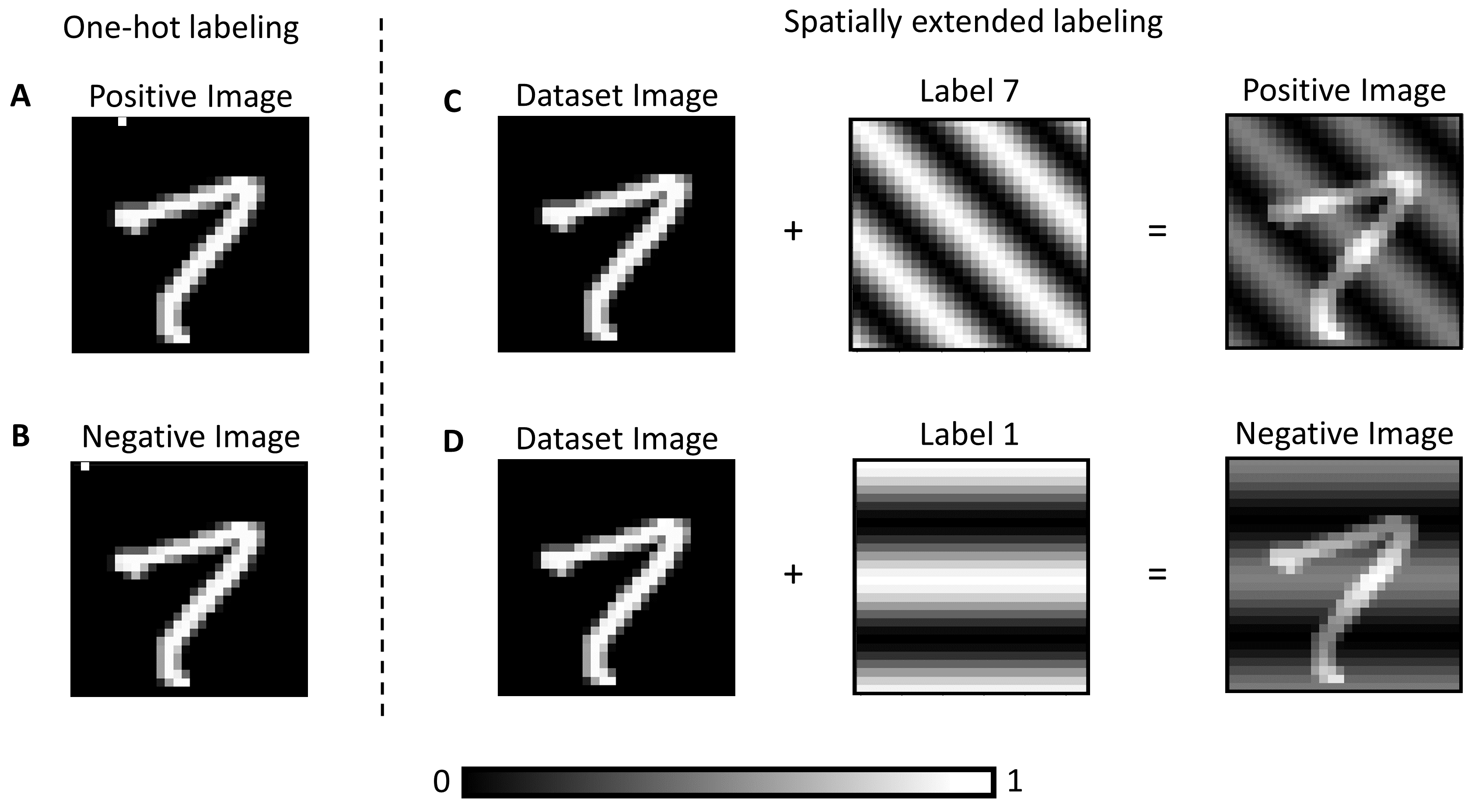
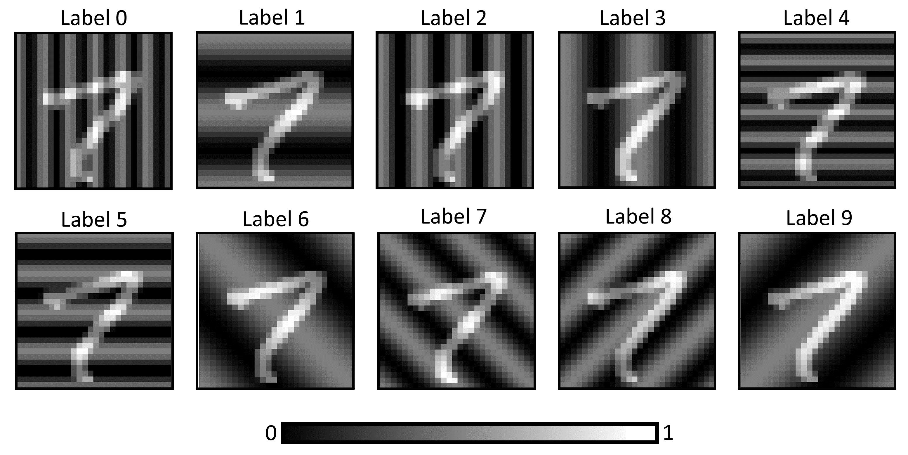
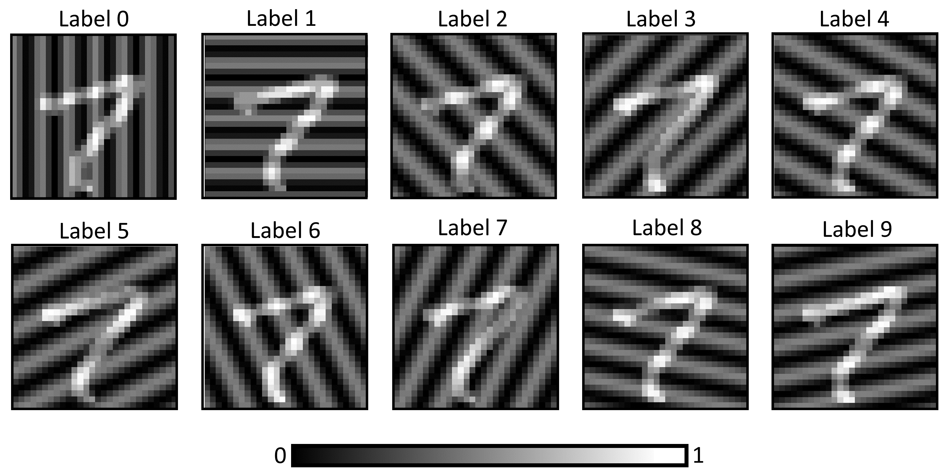
Here, we introduce a spatial-extended labeling approach involving the superposition of the training data set image with a second image of identical dimensions. This additional image consists of a gray-value wave with a fixed frequency, phase, and orientation. Each possible label is associated with a distinct configuration of these three parameters. As indicated in Figure 1C and Figure 1D, both the positive and negative data sets are obtained by harnessing this methodology. Labels are created by starting from an empty 2D Fourier space of the same size than the image. We then set a single 2D Fourier mode to a finite amplitude. The mapping between the labels and the wavelength and orientation of the corresponding mode is a matter of choice; we have tested two different options. Set 1, which is reported in Figure 2, is characterized by a combination of 4 different wave orientations (0°, 45°, 90°, 135°) and three different frequencies. Set 2, as shown in Figure 8, Appendix A, uses only one spatial frequency and obtains the different labels from ten equidistant angular orientations in the range [0°, 180°]. The results obtained by set 2 are slightly worse, which we report in Appendix A. After the label superposition, the images are normalized to the range [0, 1]. The relative contribution $K$ of the label pattern to the total intensity of the image is a hyperparameter, whose influence will be described in Section 3.2.3. Note that we choose our negative labels randomly, not specifically hard based on another forward pass, as it suggested in Hinton (2022).

Figure 2: Superposition of an image of the digit 7 with the full first set of waves used for the spatially-extended labeling. Only the image with the label 7 is part of the positive data set, while one of the other nine images is randomly selected to be part of the negative data set.

2.2 Implementation of the learning algorithm

The present study uses a network architecture composed of three consecutive FF-trained convolutional layers. All three layers contain the same number of filter matrices, which is one of the hyperparameter we examine. We did not add any max pooling layers because we found that those decrease accuracy as described in Appendix C. Additionally, all neurons use ReLU as activation function. All results reported are obtained using the MNIST handwritten digits data set (LeCun and Cortes (2010)). We split the original training data into 50,000 images used for training and 10,000 validation images used in the search for the optimal hyperparameters. All reported validation accuracy values are averaged over 5 independent runs with standard deviations typically being 0.01%. The original 10,000 test images were only used for obtaining the final result reported in Section 3.1.

Just as in the FF training of DNNs, we evaluate the loss of each convolutional layer by computing the sigmoidal function $\sigma$ of the goodness. The goodness is defined as the sum of squared layer activations $y_{i}$, modified by subtracting a user-provided threshold $\theta$. Following the code provided by Geoffrey Hinton, and as confirmed by Gandhi et al. (2023), we choose $\theta$ to be equal to the number of neurons $N$ within that layer. While computing the loss, we have to account for our different objectives regarding positive and negative data as:

$${loss}_{\,layer}=\sigma\left(\sum_{i=1}^{N}\begin{cases}y_{i}^{2}-\theta&\text{if positive data}\\ -y_{i}^{2}+\theta&\text{if negative data}\end{cases}\right).$$

Note that we do not induce symmetry in our loss as described in Lee and Song (2023). But we took inspiration from Lorberbom et al. (2023), who found improved collaboration between layers by training them with a cumulative network loss, which was computed by summing the individual layer losses obtained from ${loss}_{\,layer}$. Here, we exclude the loss of the first layer since it yielded better accuracy, as shown in Appendix B. This also aligns with Hinton’s exclusion of the first layer during the evaluation phase Hinton (2022).

We follow the implementation of Hinton (2022) in two more aspects. First, we apply layer normalization between the individual layers. As described in Ba et al. (2016), layer normalization involves the application of the following transformation to each activation $y_{i}$ as:

$$y_{i,norm}=y_{i}\bigg{/}{\left(\sqrt{\frac{\sum^{N}_{i=1}y_{i}^{2}}{N}}\right)}.$$

This assures that each subsequent layer can only use the pattern, not the norm of the matrix formed by the activations of the previous layer. Second, the learning rate $lr$ is modified halfway through the epochs by employing a linear cooldown:

$${lr}(e)=\frac{2\;{lr}}{E}\left(1+E-e\right),$$

where $E$ represents the total number of epochs and $e$ is the current epoch. In order to study the contribution of the individual layers, we define a layer based loss and accuracy which measures only the capability to discriminate between images of the positive and negative data set. We interpret the output of the Sigmoid function as a probability, where values greater than $0.5$ indicate that the layer recognizes the image as belonging to the positive data set. By comparing with the true assignation (positive or negative), we obtain a discrimination accuracy. Lastly, by using the probability to compute a binary cross entropy, we compute a layer-specific discrimination loss.

2.3 Two ways of inference

There are two ways how a FF trained CNN or DNN can be used for inference: the linear classifier and the goodness evaluation. In the first case, $H$ neurons of every layer (except the first) are fully-connected with an output layer of $N$ nodes, equal to the number of labels. The connecting weights, $H$ times $N$ in number, are trained by evaluating the neuron activations using a cross-entropy loss. This is the default method of inference used in this paper, unless mentioned otherwise. For inference with goodness evaluation, each image is exposed $N$ times to the neural network, each time superimposed with another of the $N$ possible labels, and the goodness parameter is computed for each label $m$. The image is then associated with ${label}_{\,correct}$, which is the label characterized by the highest goodness value, and is defined as:

$${label}_{\,correct}=\text{argmax}\left(\begin{bmatrix}f_{0}\\ f_{1}\\ \vdots\\ f_{8}\\ f_{9}\end{bmatrix}\right),$$

where for each associated label $m$, the goodness is expressed as $f_{m}=\sum^{H}_{i=1}y_{i}^{2}$, and $H$ is the number of all neurons, except those from the first layer.

2.4 Hardware and software

The code for our FF trained CNN is implemented in Python using the PyTorch library (pytorch). The source code of Loewe (2023) for an FF trained, fully connected DNN was used as the starting point, and our code is available on GitHub. All analysis presented here was performed on a desktop workstation with an AMD Ryzen 9 5900X 12-Core Processor with 128 GB RAM, and an NVIDIA GeForce RTX 3080 GPU with dedicated 12 GB RAM.

3 Results

We first report the configuration which achieved the highest accuracy, followed by the search through the space of hyperparameters (using only our validation data set) leading to the optimal configuration. We close by demonstrating the ability of FF trained CNNs to implement Class Activation Maps, which is a method from the explainable AI toolbox.

3.1 Performance of the optimized configuration

The hyperparameter optimization leads to the following configuration for the FF trained CNN: three convolution layers of each 128 filters with a kernel dimension of 7x7 pixels. After training for 200 epochs with a batch size of 50 using the Adam optimizer with a learning rate of $5\times 10^{-5}$, and the label set 1 (Figure 2) with intensity $K$ of 35%, we obtain 99.20% accuracy for the validation data set and 99.16% for the test data set using the goodness approach for inference. While having a significantly shorter run time, inference with the linear classifier approach provides slightly worse results, achieving accuracy values of 99.14% and 99.00% for validation and test data sets, respectively. For comparison, using again a three layer CNN of constant size, but trained with BP, we obtain a validation accuracy of 99.13%. Here the search for optimal hyperparameters resulted in 16 filters of 5x5 pixels, Adam optimizer with learning rate of $10^{-3}$, 200 epochs with batch size of 50.

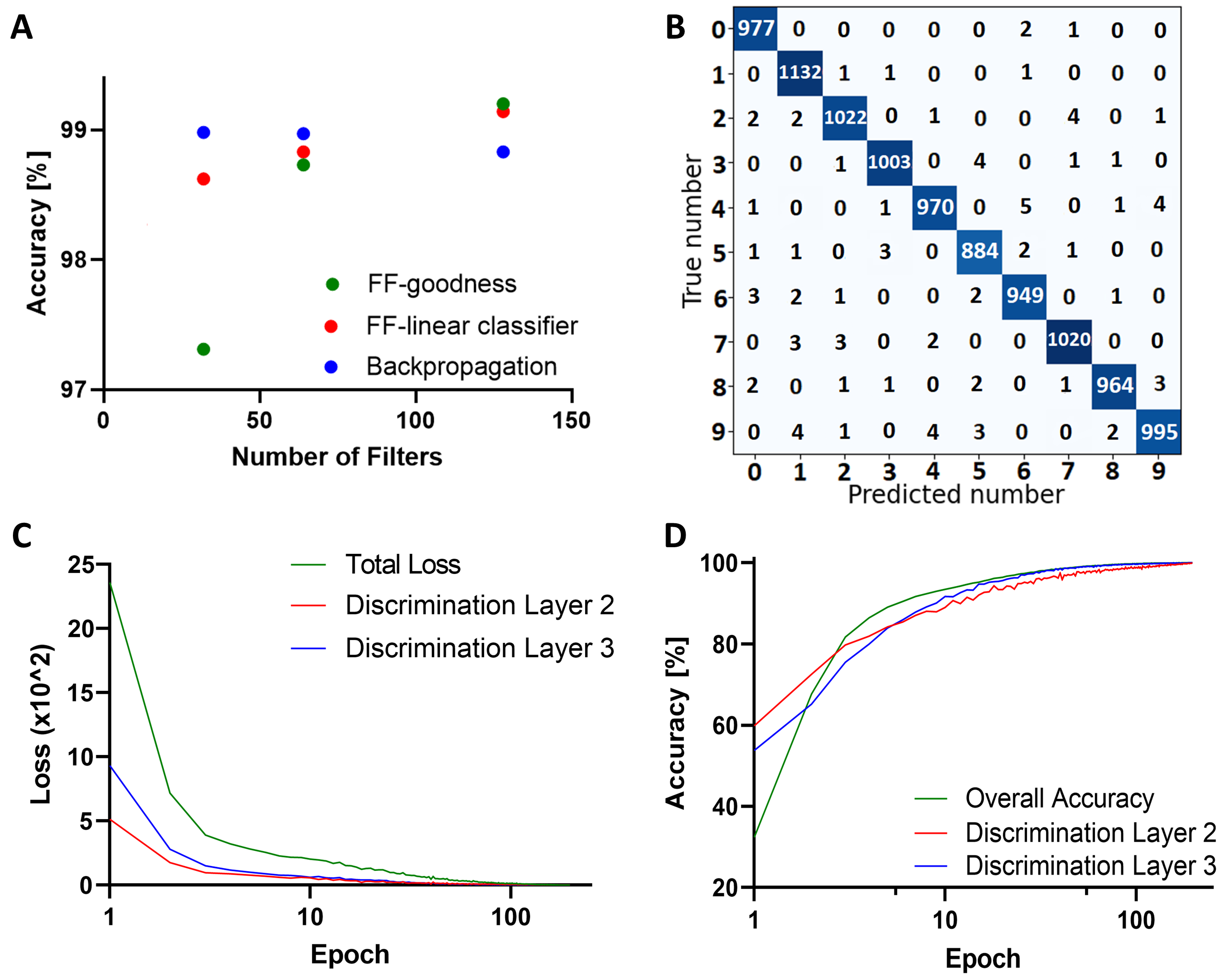
Figure 3 provides a more detailed picture of this comparison. Figure 3A shows that the performance of FF training increases monotonously with the number of filters per layer, while BP training accuracy decreases slightly under the same conditions. The latter is most likely due to increasing overfitting; its absence indicates that FF training might either be more robust against overfitting, or that it makes less efficient use of its number of trainable parameters. The confusion matrix in Figure 3B provides insight into the classification performance, revealing that labels 4 and 9 exhibit the least accurate classifications (lower than 98.70%), while labels 1, 3 and 7 are characterized by the highest accuracy levels (higher than 99.20%). After 200 epochs, the discrimination loss of the FF trained network reaches a plateau for all considered layers (Figure 3C). This convergence of the training is confirmed by a training run with 750 epochs which results in no further substantial changes in accuracy. Moreover, the accuracy value on the training data reaches close to 100% (depicted in Figure 3D with a green line) for 200 epochs. The discrimination accuracy values of the layers (red and blue lines in Figure 3D) corroborate this result. They also hint at a slightly different interplay between the dynamics of layers 2 and 3, with layer 2 initially learning faster, but layer 3 achieving a higher faculty of discrimination on the long run.

Figure 3: The best MNIST performance of an FF-trained CNN architecture is comparable to the results of a backpropagation trained CNN of the same architecture. (A) shows the accuracy values obtained for CNN with three convolutional layers as a function of the number of filters in each layer, after being trained for 200 epochs with batch size 50. Filter size is 7x7, the learning rate is set to the respective optimal value of $5\times 10^{-5}$ for FF and $10^{-3}$ for BP. FF trained networks use labels from set 1 and a label intensity $K$ of 35% (our defaults). The values reported for BP and FF are gathered from the validation data. The green data points shows the results related to the FF trained network, with inference using the goodness comparison. In this scenario, 99.16% accuracy was achieved with 128 filters per layer using the test data as shown by the corresponding confusion matrix reported in (B). (C) shows the loss computed for the discrimination between positive and negative training data for each hidden layer contributing to the training (red and blue lines), and the combined loss used during training (green line). (D) displays the discrimination accuracy of the same hidden layers (red and blue lines), and the total accuracy obtained during training (green line).

3.2 Influence of hyperparameters

This section discusses the search for optimal hyperparameters we performed in order to obtain the result reported in Section 3.1. The performance of BP trained neural networks depends on the specific value of the hyperparameters used during training. There is no reason to expect this to be different for FF training. This search also included the exploration of some architectural options which are not hyperparameters in the strict sense. We limited our search to networks of three layers of convolutional filters, all with the same number of filters per layer. Moreover, we did not include max pooling layers, because the tests described in Appendix C indicate that they decrease accuracy. For the choice of an optimizer, we tested Stochastic Gradient Descent and Adam optimizer, with the latter consistently outperforming the former. For the learning rate of Adam optimizer, we evaluated the range between $10^{-2}$ and $10^{-7}$. A learning rate of $5\times 10^{-5}$ yielded the best results and was therefore chosen as default. As in Section 3.1, we found that after training for 200 epochs the network had converged in all configurations tested, which made this value also our default.

3.2.1 Filter dimensions, layer width, and batch size

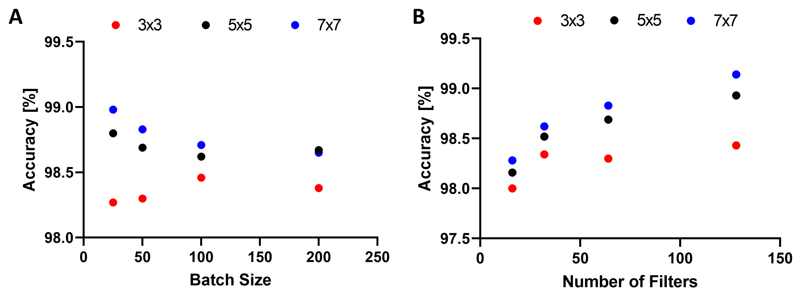
First, we describe the interaction of the two architectural parameters, namely, filter dimension and number of neurons in each layer with the training parameter batch size. Figure 4A shows that the accuracy decreases with lower filter size. A possible explanation is that the smaller filters have more problems in identifying the wavelengths of the label waves. For 7x7 and 5x5 filters we additionally observe an increase in accuracy for smaller batch sizes. We speculate that this might be a generic feature due to the dual nature of the training data. Figure 4B confirms the increase of accuracy with the number of filters per layer for all filter sizes, which was first shown in Figure 3A, with the accuracy decreasing with smaller filter size.

Figure 4: FF-trained CNN benefits from small batch sizes and a large number of filters. (A) Accuracy as a function of batch size and filter size (3x3, 5x5, or 7x7 pixels) in a network of three layers of each 64 filters. (B) Accuracy values obtained by varying the number of filters per layer (16, 32, 64, 128) and the filter size using a batch size of 50.

3.2.2 Inference: linear classifier vs. goodness approach

As described in Section 2.2 there are two ways for making inference with a FF trained neural network. Table 1 shows that the goodness computation approach beats the linear classifier over a variety of different CNN hyperparameters configurations, and this finding agrees with the proposal of Hinton (2022) and the result of Brenig and Timofte (2023). However, the slightly superior results go together with a ten times larger computational cost of the goodness comparison, because each image in the data set must be processed for each label in order to perform the classification task. Consequentially, the goodness approach might only be justified for classification task with a limited number of labels.

FF-CNN Network	Linear Classifier	Goodness
	Accuracy [%]	Accuracy [%]
128 filter of size 7x7, batch size 50	99.14	99.20
128 filter of size 5x5, batch size 50	98.93	99.04
128 filter of size 3x3, batch size 25	98.63	98.74

Table 1: Using the goodness approach yields a higher accuracy during inference than the linear classifier, albeit at 10 times higher computational cost. Three different sets of hyperparameters were trained, with the best results highlighted in bold.

3.2.3 Effect of the relative labeling intensity K

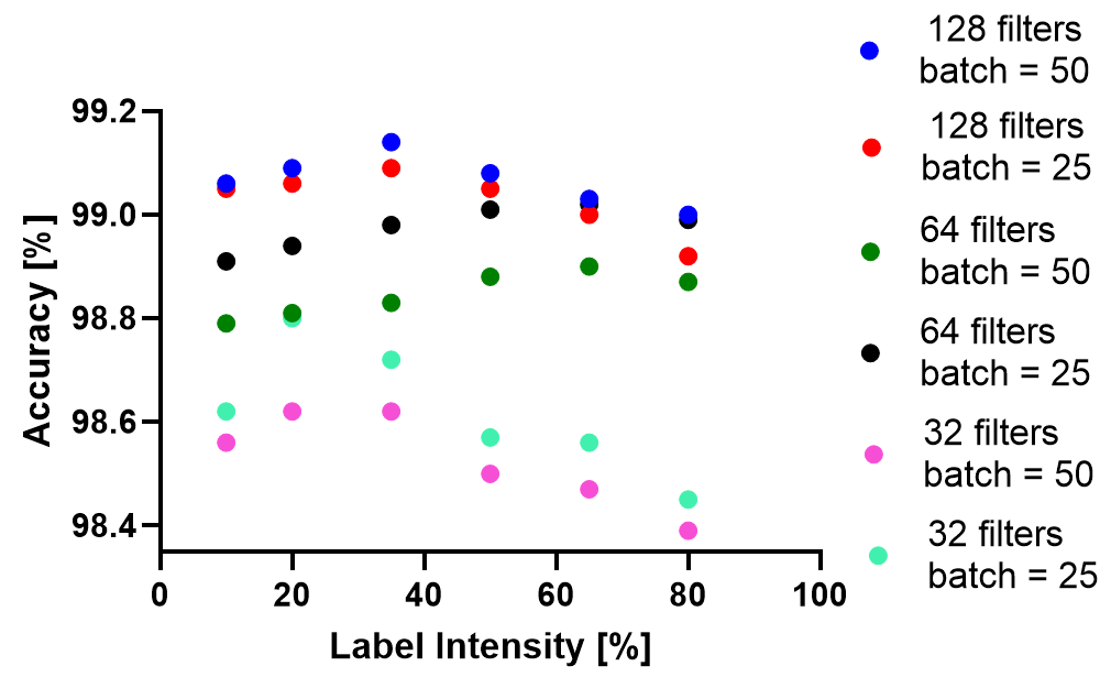
In studying the effect of the relative label intensity $K$, we focus on the hyperparameters that exhibit the highest accuracy values: 32, 64 or 128 convolutional filters per layer, filter size 7x7, and batch sizes of 25 and 50 images. The results presented in Figure 5 show that optimizing $K$ leads to an increase in accuracy of up to 0.2%. The optimal value of $K$ does depend on layer width but not on batch size. Specifically, the 32 neurons per layer architectures achieves the highest accuracy for $K$ approximately $20\%$, for 64 neurons per layer the optimal $K$ increases to approximately $65\%$, for 128 neurons per layer it drops again to approximately $35\%$. This non-monotonic behaviour does not lend itself to a simple explanation.

Figure 5: The best choice of the relative label intensity $K$ depends on the filter number and batch size. All accuracy values are obtained for training with 7x7 filter size.

3.3 Class activation maps

Class Activation Maps (CAMs) are visual representations that highlight the regions of an input image which contribute most to the prediction of a given label. CAMs are obtained by summing up the feature maps generated by the convolutional layers, each weighted with the corresponding weights associated with a specific label. The main underlying idea is that each feature map decodes specific spatial characteristics of the input image, and as a result, the weights quantify how much these characteristics contributes to the recognition of the target class. In BP trained CNNs, CAMs are typically obtained by applying a global average pooling layer after the last convolutional layer, followed by using the weights connecting this layer to a Softmax activation output layer.

Here we train a CNN with FF and a linear classifier for inference. The weights of the linear classifier connecting the individual pixels in our feature map with the set of ten output neurons are exactly the weights we need to assess the role of the corresponding pixel for a given prediction. Figure 6 provides four examples of CAMs of correctly identified images. For the digit 1, (Figure 6A and Figure 6B) the entire vertical shape contributes to the correct inference. In contrast, for the digit 2 in Figure 6C three distinct areas (the upper, the bottom-left and the bottom right parts of the number) contribute to the correct labeling. Similarly expressive regions can be identified for the digits 7 and 9 in Figure 6E and Figure 6G.

Figure 6: Class activation maps (CAMs) of a FF trained CNN show which image regions are considered beneficial (yellow) or deleterious (pink) by the network for making its prediction. (A), (C), (E), and (G) display four input images. (B), (D), (F), and (H) are their corresponding CAMs. All examples are from a network with 16 convolutional neurons per layer, filter size 5x5, and trained with a batch size of 50.

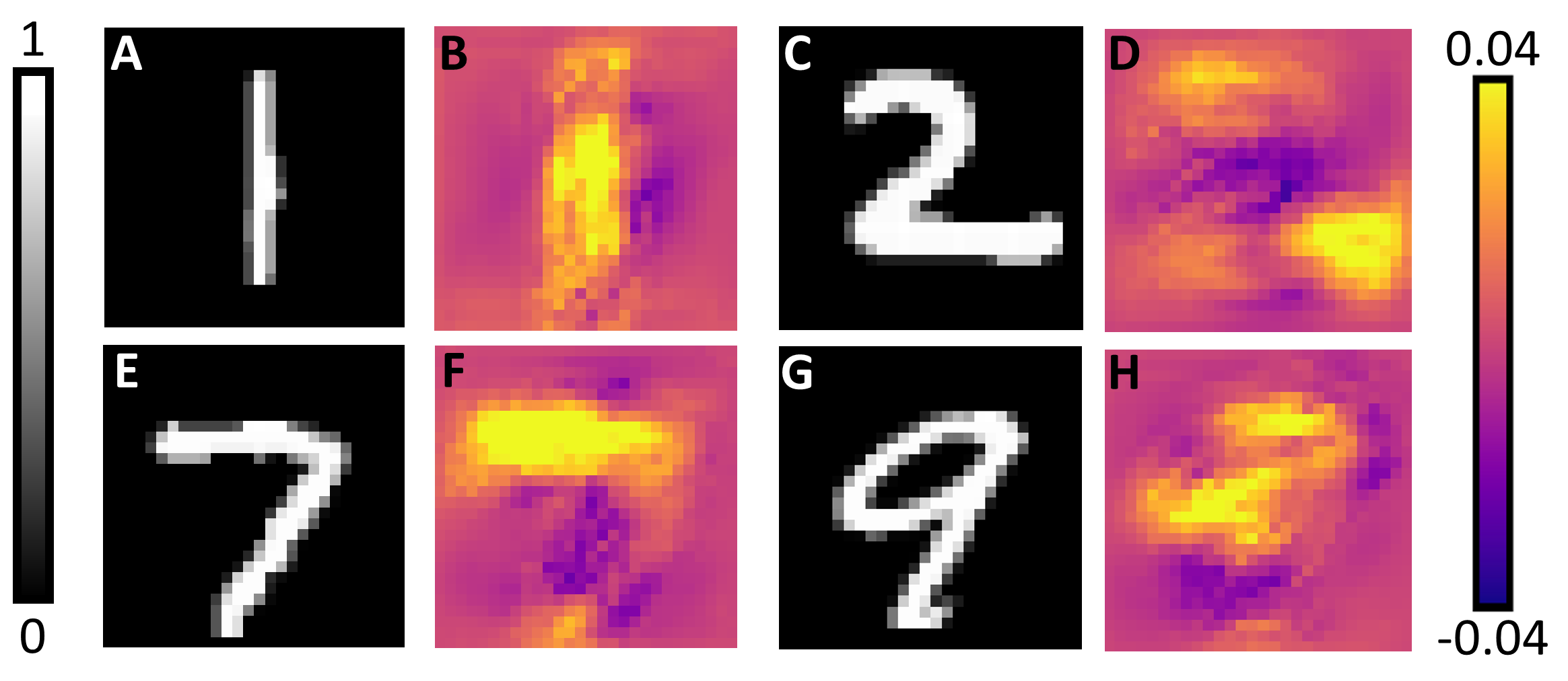
CAMs also show that the different layers of the FF trained CNN provide similar, but distinct information for the classification task. For instance, when considering the digit 7 in Figure 7, the second layer of the network provides more information on the inner portion of the horizontal line, while the third layer responds more to the boundaries of that horizontal line.

Figure 7: Class activation maps show that the different layers of the FF-trained CNN provide similar, but yet distinguishable information. (A) shows the CAM obtained from considering both layer 2 and layer 3 together. (B) and (C) show the CAMs obtained respectively only from layer 2 and layer 3.

4 Discussion and conclusions

CNNs are considered the gold standard in deep learning-based image analysis. For instance, in biomedical imaging, they overcome the drawbacks of subjective analysis in the semi-quantitative visual inspection of samples (Gurcan et al., 2009), and they support experts during their daily clinical routine by reducing their workload (Shmatko et al., 2022). Furthermore, their exploitation of the spatial information within images makes them suitable for the deployment of explainable AI tools (such as class activation maps), which highlight the image regions contributing most significantly to the classification outcome. Our implementation of FF trained CNN shows that with the right choice of hyperparameters, this technique is competitive with backpropagation. These results were obtained without implementing all the possible and suggested optimizations such as enforcing symmetry of the loss function (Lee and Song, 2023) or choosing hard, i.e. easily confused, labels for the negative data set, as suggested by Hinton (2022). We propose that our work shows the potential of FF trained CNNs to address real world computer vision problems. An open question remains if this technique will supersede BP in specific applications. We believe that this potential exists, especially in the cases of neuromorphic hardware and unsupervised learning.

A better understanding of the FF training will however also expand our understanding of the generic concept of neuronal information processing in all its breadth from biological systems to reservoir computing. The demonstrated capability to implement class activation maps offers an initial insight into these research topics. Achieving deeper insights will also mean to understand how the two innovations of FF, providing positive and negative labels and computing a locally defined goodness parameter, contribute to its success individually and synergetically (Tosato et al., 2023). Moreover, a better understanding why it is beneficial to exclude the first layer during the goodness computation (c.f. Appendix B) would be desirable. Subsequent work on FF training should also address its ability to train deeper networks, most likely expanding on the work of Lorberbom et al. (2023). Also the ability of FF training to work with larger and more complex data sets needs to be explored. Finally, its connection to biological neuronal systems (Ororbia and Mali, 2023; Ororbia, 2023) seems a promising research direction.

Acknowledgments and Disclosure of Funding

This project has received funding from the Innovative Medicines Initiative 2 Joint Undertaking (JU) under grant agreement number 101034427. The JU receives support from the European Union’s Horizon 2020 research and innovation program and EFPIA. The JU is not participating as a contracting authority in this procurement. This project was also funded by the Ministry for Science and Culture of Lower Saxony as part of the project “Agile, bio-inspired architectures” (ABA). The authors also thank Christian Dullin for insightful discussions.

Appendix A A second way of encoding the labels

For further information, refer to Figure 8 and Table 2.

Figure 8: Label set 2 superimposed on an image of the digit 7. The 10 different labels shown here share the same wavelength and differ only in their orientation. Only the label 7 from the MNIST data set is a part of the positive data set, while one image from the 10 images shown is randomly selected for the negative data set.

FF-CNN Network	Set 1 labels Acc. [%]	Set 2 labels Acc. [%]
32 filters of size 3x3, batch size 50	98.34	98.36
32 filters of size 7x7, batch size 25	98.72	98.53
64 filters of size 3x3, batch size 50	98.30	98.22
128 filters of size 3x3, batch size 50	98.43	98.38

Table 2: FF trained CNNs achieve higher accuracy values when labeled with set 1 instead of set 2. Four different sets of hyperparameters were trained, with the best results highlighted in bold.

Appendix B Contribution of the first layer

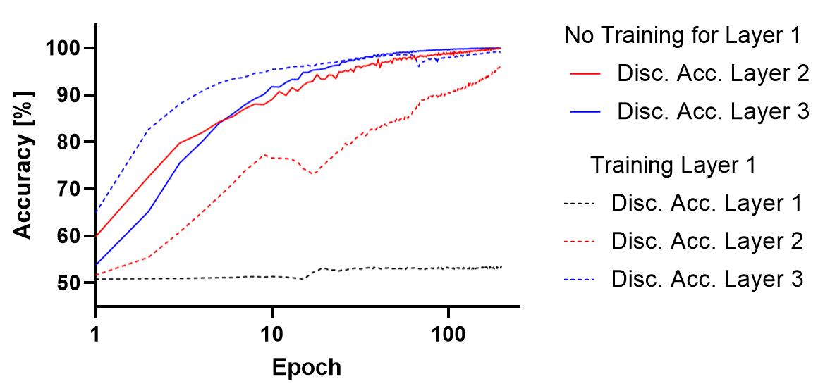
In order to investigate the effect of the goodness of the first convolutional layer, we train the CNN configurations reported in Section 3.1 again, but this time including the first layer in the goodness computation. Figure 9, reports the results, highlighting that the training of the first layer affects the the speed of convergence of the next layers. Adding the first layer also reduces the overall accuracy of the network by approximately 2%.

Figure 9: Our implementation of FF trained CNNs does not require the inclusion of the goodness of the first layer during training. Continuous lines represent evolution of the discrimination accuracy during the training phase, when the first layer is not included. Dashed lines represent the discrimination accuracy evolution if its goodness is included.

Appendix C Effect of max pooling

We also examine how max pooling layers influence FF trained CNNs by testing five different configurations and increased architectonic complexity by having higher number of filters for increasing layer number. As shown in Table 3, our analysis exhibits a decrease in accuracy when max pooling layers were applied, suggesting that preserving the entire information is preferable.

FF-CNN Network	FF Acc. [%]	FF + MaxPooling Acc. [%]
128 filters of size 7x7	99.14	98.97
16 filters of size 5x5	98.16	97.57
64 filters of size 3x3	98.30	98.18
32, 64, 128 filters of size 7x7	98.90	98.54
16, 32, 64 filters of size 7x7	98.47	98.22

Table 3: Adding max pooling layers reduces the performance of FF trained CNN. Five sets of hyperparameters were trained using either only three convolutional layers, or by interleaving each pair of convolutional layers with a max pooling layer. Unlike the rest of the paper, the last two configurations have different numbers of convolutions in the three layers. Batch size is 50 and a linear classifier is used for inference. Five different sets of hyperparameters were trained, with the best results highlighted in bold.

References

- Ba et al. (2016) Jimmy Lei Ba, Jamie Ryan Kiros, and Geoffrey E. Hinton. Layer normalization. arXiv.1607.06450, 2016.
- Baydin et al. (2022) Atılım Güneş Baydin, Barak A. Pearlmutter, Don Syme, Frank Wood, and Philip Torr. Gradients without backpropagation. arXiv:2202.08587, 2022.
- Brenig and Timofte (2023) Jonas Brenig and Radu Timofte. A study of forward-forward algorithm for self-supervised learning. arXiv:2309.11955, 2023.
- Christensen et al. (2022) Dennis V. Christensen, Regina Dittmann, Bernabe Linares-Barranco, Abu Sebastian, Manuel Le Gallo, Andrea Redaelli, Stefan Slesazeck, Thomas Mikolajick, Sabina Spiga, Stephan Menzel, Ilia Valov, Gianluca Milano, Carlo Ricciardi, Shi-Jun Liang, Feng Miao, Mario Lanza, Tyler J. Quill, Scott T. Keene, Alberto Salleo, Julie Grollier, Danijela Marković, Alice Mizrahi, Peng Yao, J. Joshua Yang, Giacomo Indiveri, John Paul Strachan, Suman Datta, Elisa Vianello, Alexandre Valentian, Johannes Feldmann, Xuan Li, Wolfram H. P. Pernice, Harish Bhaskaran, Steve Furber, Emre Neftci, Franz Scherr, Wolfgang Maass, Srikanth Ramaswamy, Jonathan Tapson, Priyadarshini Panda, Youngeun Kim, Gouhei Tanaka, Simon Thorpe, Chiara Bartolozzi, Thomas A. Cleland, Christoph Posch, ShihChii Liu, Gabriella Panuccio, Mufti Mahmud, Arnab Neelim Mazumder, Morteza Hosseini, Tinoosh Mohsenin, Elisa Donati, Silvia Tolu, Roberto Galeazzi, Martin Ejsing Christensen, Sune Holm, Daniele Ielmini, and N. Pryds. 2022 roadmap on neuromorphic computing and engineering. Neuromorphic Computing and Engineering, 2:022501, 2022. doi: 10.1088/2634-4386/ac4a83.
- De Vita et al. (2023) Fabrizio De Vita, Rawan M. A. Nawaiseh, Dario Bruneo, Valeria Tomaselli, Marco Lattuada, and Mirko Falchetto. µ-FF: On-Device Forward-Forward Training Algorithm for Microcontrollers. In 2023 IEEE International Conference on Smart Computing (SMARTCOMP), pages 49–56, 2023. doi: 10.1109/SMARTCOMP58114.2023.00024.
- Dellaferrera and Kreiman (2022) Giorgia Dellaferrera and Gabriel Kreiman. Error-driven input modulation: Solving the credit assignment problem without a backward pass. In Proceedings of the 39th International Conference on Machine Learning, Proceedings of Machine Learning Research, pages 4937–4955, 2022.
- Farinha et al. (2023) Matilde Tristany Farinha, Thomas Ortner, Giorgia Dellaferrera, Benjamin Grewe, and Angeliki Pantazi. Efficient biologically plausible adversarial training. arXiv:2309.17348, 2023.
- Flügel et al. (2023) Katharina Flügel, Daniel Coquelin, Marie Weiel, Charlotte Debus, Achim Streit, and Markus Götz. Feed-forward optimization with delayed feedback for neural networks. arXiv:2304.13372, 2023.
- Gandhi et al. (2023) Saumya Gandhi, Ritu Gala, Jonah Kornberg, and Advaith Sridhar. Extending the forward forward algorithm. arXiv:2307.04205, 2023.
- Gurcan et al. (2009) Metin N. Gurcan, Laura E. Boucheron, Ali Can, Anant Madabhushi, Nasir M. Rajpoot, and Bulent Yener. Histopathological image analysis: A review. IEEE Reviews in Biomedical Engineering, 2:147–171, 2009. doi: 10.1109/RBME.2009.2034865.
- Hinton (2022) Geoffrey Hinton. The forward-forward algorithm: Some preliminary investigations. arXiv:2212.13345, 2022.
- Hugging Face Community (2023) The Hugging Face Community. Anatomy of model’s memory, 2023. URL https://huggingface.co/docs/transformers/v4.36.0/model_memory_anatomy#anatomy-of-models-memory.
- Journé et al. (2023) Adrien Journé, Hector Garcia Rodriguez, Qinghai Guo, and Timoleon Moraitis. Hebbian deep learning without feedback. arXiv:2209.11883, 2023.
- LeCun and Cortes (2010) Yann LeCun and Corinna Cortes. MNIST handwritten digit database, 2010. URL http://yann.lecun.com/exdb/mnist/.
- Lee and Song (2023) Heung-Chang Lee and Jeonggeun Song. Symba: Symmetric backpropagation-free contrastive learning with forward-forward algorithm for optimizing convergence. arXiv:2303.08418, 2023.
- Lillicrap et al. (2020) Timothy P. Lillicrap, Adam Santoro, Luke Marris, Colin J. Akerman, and Geoffrey Hinton. Backpropagation and the brain. Nature Reviews Neuroscience, 21(6):335–346, 2020. doi: 10.1038/s41583-020-0277-3.
- Loewe (2023) Sindy Loewe. The Forward-Forward Fully-Connected Network Implementation, 2023. URL https://github.com/loeweX/Forward-Forward.
- Lorberbom et al. (2023) Guy Lorberbom, Itai Gat, Yossi Adi, Alex Schwing, and Tamir Hazan. Layer collaboration in the forward-forward algorithm. arXiv:2305.12393, 2023.
- Malladi et al. (2023) Sadhika Malladi, Tianyu Gao, Eshaan Nichani, Alex Damian, Jason D. Lee, Danqi Chen, and Sanjeev Arora. Fine-tuning language models with just forward passes. arXiv:2305.17333, 2023.
- McCaughan et al. (2023) Adam N. McCaughan, Bakhrom G. Oripov, Natesh Ganesh, Sae Woo Nam, Andrew Dienstfrey, and Sonia M. Buckley. Multiplexed gradient descent: Fast online training of modern datasets on hardware neural networks without backpropagation. APL Machine Learning, 1, 2023. doi: 10.1063/5.0157645.
- Nøkland (2016) Arild Nøkland. Direct Feedback Alignment Provides Learning in Deep Neural Networks. In D. Lee, M. Sugiyama, U. Luxburg, I. Guyon, and R. Garnett, editors, Advances in Neural Information Processing Systems, volume 29. Curran Associates, Inc., 2016.
- Oguz et al. (2023) Ilker Oguz, Junjie Ke, Qifei Weng, Feng Yang, Mustafa Yildirim, Niyazi Ulas Dinc, Jih-Liang Hsieh, Christophe Moser, and Demetri Psaltis. Forward–forward training of an optical neural network. Opt. Lett., 48(20):5249–5252, 2023. doi: 10.1364/OL.496884.
- Ororbia (2023) Alexander Ororbia. Contrastive-signal-dependent plasticity: Forward-forward learning of spiking neural systems. arXiv:2303.18187, 2023.
- Ororbia and Mali (2023) Alexander Ororbia and Ankur Mali. The predictive forward-forward algorithm. arXiv:2301.01452, 2023.
- Paheding and Reyes-Angulo (2023) Sidike Paheding and Abel A. Reyes-Angulo. Forward-forward algorithm for hyperspectral image classification: A preliminary study. arXiv:2307.00231, 2023.
- Paliotta et al. (2023) Daniele Paliotta, Mathieu Alain, Bálint Máté, and François Fleuret. Graph neural networks go forward-forward. arXiv:2302.05282, 2023.
- Rawat and Wang (2017) Waseem Rawat and Zenghui Wang. Deep Convolutional Neural Networks for Image Classification: A Comprehensive Review. Neural Computation, 29(9):2352–2449, 2017. doi: 10.1162/neco˙a˙00990.
- Reyes-Angulo and Paheding (2023) Abel Reyes-Angulo and Sidike Paheding. The forward-forward algorithm as a feature extractor for skin lesion classification: A preliminary study. arXiv:2307.00617, 2023.
- Rumelhart et al. (1986) David E. Rumelhart, Geoffrey E. Hinton, and Ronald J. Williams. Learning representations by back-propagating errors. Nature, 323(6088):533–536, 1986.
- Scellier and Bengio (2017) Benjamin Scellier and Yoshua Bengio. Equilibrium Propagation: Bridging the Gap between Energy-Based Models and Backpropagation. Frontiers in Computational Neuroscience, 11, 2017. doi: https://doi.org/10.3389/fncom.2017.00024.
- Shmatko et al. (2022) Artem Shmatko, Narmin Ghaffari Laleh, Moritz Gerstung, and Jakob Nikolas Kather. Artificial intelligence in histopathology: enhancing cancer research and clinical oncology. Nature Cancer, 3(9):1026–1038, 2022. doi: 10.1038/s43018-022-00436-4.
- Tosato et al. (2023) Niccolò Tosato, Lorenzo Basile, Emanuele Ballarin, Giuseppe de Alteriis, Alberto Cazzaniga, and Alessio Ansuini. Emergent representations in networks trained with the forward-forward algorithm. arXiv:2305.18353, 2023.
- Weber et al. (2023) Leander Weber, Jim Berend, Alexander Binder, Thomas Wiegand, Wojciech Samek, and Sebastian Lapuschkin. Layer-wise feedback propagation. arXiv:2308.12053, 2023.
- Yang (2023) Yukun Yang. A theory for the sparsity emerged in the forward forward algorithm. arXiv:2311.05667, 2023.
- Zhao et al. (2023a) Gongpei Zhao, Tao Wang, Yidong Li, Yi Jin, Congyan Lang, and Haibin Ling. The cascaded forward algorithm for neural network training. arXiv:2303.09728, 2023a.
- Zhao et al. (2023b) Yequan Zhao, Xinling Yu, Zhixiong Chen, Ziyue Liu, Sijia Liu, and Zheng Zhang. Tensor-compressed back-propagation-free training for (physics-informed) neural networks. arXiv:2308.09858, 2023b.
- Zhou (2022) Hongchao Zhou. Activation learning by local competitions. arXiv:2209.13400, 2022.