Lift-Attend-Splat: Bird’s-eye-view camera-lidar fusion using transformers

Abstract

Combining complementary sensor modalities is crucial to providing robust perception for safety-critical robotics applications such as autonomous driving (AD). Recent state-of-the-art camera-lidar fusion methods for AD rely on monocular depth estimation which is a notoriously difficult task compared to using depth information from the lidar directly. Here, we find that this approach does not leverage depth as expected and show that naively improving depth estimation does not lead to improvements in object detection performance and that, strikingly, removing depth estimation altogether does not degrade object detection performance. This suggests that relying on monocular depth could be an unnecessary architectural bottleneck during camera-lidar fusion. In this work, we introduce a novel fusion method that bypasses monocular depth estimation altogether and instead selects and fuses camera and lidar features in a bird’s-eye-view grid using a simple attention mechanism. We show that our model can modulate its use of camera features based on the availability of lidar features and that it yields better 3D object detection on the nuScenes dataset than baselines relying on monocular depth estimation.

1 Introduction

Integrating information from different modalities efficiently and effectively is especially important in safety-critical applications such as autonomous driving, where different sensor modalities are complementary and combining them adequately is crucial to guarantee safety. For example, cameras capture rich semantic information of objects up to far away distances, while lidars provide extremely accurate depth information but are sparse at large distances. For this reason, many modern self-driving platforms have a large number of different sensors which must be combined together in order to provide accurate and reliable perception of the surrounding scene and allow safe deployment of these vehicles in the real world.

Multimodal sensor fusion — learning a unified representation of a scene derived from multiple sensors — offers a plausible solution to this problem. However, training such multimodal models can be challenging, especially when modalities are as different as cameras (RGB images) and lidars (3D point clouds). For instance, it is known that different modalities overfit and generalise at different rates [53] and that training all modalities jointly can lead to underutilisation of the weaker modalities and even to inferior results compared to unimodal models in some situations [37].

In the context of autonomous driving, many of the recent state-of-the-art methods for camera-lidar fusion [33, 28, 14] are based on the Lift-Splat (LS) paradigm [38]. In this approach, the camera features are projected in bird’s-eye-view (BEV) — or top-down space — using monocular depth before being fused with the lidar features. As a result, the location of the camera features in BEV is highly dependent on the quality of the monocular depth prediction and it has been argued that its accuracy is critical [28, 14]. In this work we reconsider these claims and show that the monocular depth prediction inside these models is of poor quality and cannot account for their success. In particular, we present results showing that methods based on Lift-Splat perform equally well when the monocular depth prediction is replaced by direct depth estimation from the lidar point cloud or removed completely. This leads us to suggest that relying on monocular depth when fusing camera and lidar features is an unnecessary architectural bottleneck and that Lift-Splat could be replaced by a more effective projection mechanism.

We introduce a novel approach for camera-lidar fusion called “Lift-Attend-Splat” that bypasses monocular depth estimation altogether and instead selects and fuses camera and lidar features in BEV using a simple transformer. We present evidence that our method shows better camera utilisation compared to the methods based on moncular depth estimation and that it improves object detection performance. Our contributions are as follows:

• We show that camera-lidar fusion methods based on the Lift-Splat paradigm are not leveraging depth as expected. In particular, we show that they perform equivalently or better if monocular depth prediction is removed completely.

• We introduce a novel camera-lidar fusion method that fuses camera and lidar features in BEV using a simple attention mechanism. We show that it leads to better camera utilisation and improves 3D object detection compared to models based on the Lift-Splat paradigm.

2 Related work

3D object detection for autonomous driving

For 3D object detection, most benchmarks are dominated by methods using lidar point clouds due to their highly accurate range measurement allowing for better placement of objects in 3D compared to methods using cameras or radars only. Deep learning methods for classification on point clouds were pioneered in the seminal works of [40, 41] and early works have been applying similar ideas to 3D object detection [42, 45]. A more recent family of methods is based on direct voxelisation of the 3D space [65, 59] or compression of the lidar representation along the z-direction into “pillars” [22, 60]. These approaches have been very successful and are the basis of many follow-up works [62, 15, 19].

The task of 3D object detection has also been tackled from multiple cameras alone. Early works have mostly been based on various two-stage approaches [4, 42, 20, 54], while recent methods have been leveraging monocular depth estimation directly [3, 21, 43]. This task is difficult when lidar is absent because 3D information must be estimated using images only, which is a challenging problem. However, recent works have shown impressive performance by borrowing ideas from lidar detection pipelines [16, 7, 11], by improving position embeddings [31] and 3D queries [18], as well as by leveraging temporal aggregation [67, 12, 32, 52, 30, 25] or 2D semantic segmentation [64].

Camera-lidar fusion

Perception quality can be improved by leveraging jointly cameras and lidars when available. Recent fusion methods can be broadly classified in three categories: point decoration methods, methods that leverage task-specific object queries and architectures, and projection based methods. Point decoration methods augment the lidar point cloud using semantic segmentation data [49, 57], camera features [51], or even create new 3D points using object detections in the image plane [63]. Such methods are relatively easy to implement but suffer from the fact that they require lidar points to fuse camera features. TransFusion [1] is a recent example of a method that leverages task-specific object queries generated using the lidar point cloud. Final detections are made directly without explicit projection of camera features into BEV space. Fusion can also be performed earlier in the model, for example at the level of the 3D voxels [6, 5] or lidar features [23], or by sharing information between the camera and lidar backbones [26, 17, 39]. Finally, projection-based methods project camera features into 3D before fusing them with the lidar (see below).

Projection based methods

Of special interest to us are camera-lidar fusion methods based on projecting camera features into 3D. Recent state-of-the-art methods [33, 28, 14] which rank among the top entries in the nuScenes leaderboard [2] leverage the ideas presented in [38] and project camera features in 3D using monocular depth estimation. It was shown in [14] that the performance of [33, 28] can be boosted significantly by including features derived from the ground-truth lidar depth map into the camera stream prior to monocular depth estimation. An alternative approach is to project camera features directly into BEV space using the known correspondence between lidar points and camera features [8, 55, 23]. However, the sparsity of the lidar point cloud can limit which camera features are projected, as described in [33]. Finally, learning to project camera features in BEV without explicit depth can be achieved when lidar is absent using a transformer, as shown in [44, 25]. Here, we extend this line of work to the case of camera-lidar fusion and leverage cross-attention to generate a dense BEV grid of camera features to be fused with the lidar.

Camera

Lidar

BEVFusion [33]

BEVFusion [33] w/ $\lambda=1$

	Abs. Rel. $\downarrow$	RMSE $\downarrow$	mAP $\uparrow$
BEVFusion [33]	2.75	17.40	68.5
BEVFusion [33] w/ Eq. 2:
$\lambda=0$	2.83	18.54	68.4
$\lambda=0.001$	3.14	19.91	68.1
$\lambda=0.01$	0.76	8.09	68.0
$\lambda=0.1$	0.43	6.47	68.1
$\lambda=1$	0.22	4.77	68.1
$\lambda=5$	0.19	4.53	66.6
$\lambda=100$	0.16	4.55	64.6
Lidar	0.04	0.29	68.4
Pretrained	0.64	7.87	67.4
No depth	–	–	68.5

Figure 1: Impact of the quality of the monocular depth prediction on the object detection performance of BEVFusion [33] on the nuScenes validation set. We compare BEVFusion and four different variants: adding depth supervision using Eq. 2 with various weights $\lambda$, using lidar depth maps instead of monocular depth estimation (lidar), using a pretrained and frozen depth classifier (pretrained), and finally removing depth estimation altogether by projecting camera features at all depths uniformly using Eq. 3 (no depth). In our experiments, more accurate depth does not translate to better detection performance and the original model is on-par with using the lidar points directly as a source of depth. Equivalent detection performance was achieved using the no depth model, clearly indicating that accurate monocular depth is not necessary for BEVFusion [33] to achieve its performance, see main text and Sec. A.4 for details.

3 Monocular depth prediction in Lift-Splat

Recent camera-lidar fusion methods based on the Lift-Splat paradigm [33, 28] learn a unified representation in the form of a BEV grid by projecting camera features in BEV space using monocular depth estimation as

$$\text{Proj}_{\text{Lift-Splat}}=\text{Splat}\left({F^{\prime}}^{\text{cam}}\otimes D\right),$$ (1)

where ${F^{\prime}}^{\text{cam}}\in\mathbb{R}^{C_{c}^{\prime}\times H\times W}$ is a context vector obtained from the camera features $F^{\text{cam}}\in\mathbb{R}^{C_{c}\times H\times W}$, $D\in\mathbb{R}^{N_{D}\times H\times W}$ is a normalised distribution over predetermined depth bins and Splat denotes the operation of projecting each point downwards into the $z=0$ plane, see [33, 28, 38] for details. The resulting feature map is then merged with the lidar features using concatenation [33] or gated attention [28]. In this paradigm, monocular depth prediction is formulated as a classification problem and learned indirectly from the downstream task without explicit depth supervision.

Lift-Splat depth prediction is generally poor

We analyse the quality of the depth predicted by BEVFusion [33] by comparing it to lidar depth maps, both qualitatively and quantitatively using the absolute relative (Abs. Rel.) and root mean squared errors (RMSE) [9, 24]. As shown in the example displayed on Fig. 1, the depth prediction does not accurately reflect the structure of the scene and is markedly different from the lidar depth map which suggests that monocular depth is not leveraged as expected in [33]. More details can be found in Sec. A.2.

Improving depth prediction does not improve detection performance

We next investigate whether improving the the depth prediction quality can boost object detection performance. To do so, we retrain the model from [33] with the following loss:

$$L_{\text{total}}=L_{\text{sup}}+\lambda L_{\text{depth}},$$ (2)

where $L_{\text{sup}}$ is the original 3D object detection loss and $L_{\text{depth}}$ is a simple cross-entropy loss for the depth estimation that uses the lidar depth as a target, see Sec. A.3 for more details. By changing the hyper-parameter $\lambda$, we can control the quality of the depth prediction and explore how it impacts detection performance. In Fig. 1, we see that while depth supervision indeed leads to much more accurate depth maps both visually and quantitatively, detection performance — measured using mean average precision (mAP) — degrades from the baseline as the weight of the depth supervision is increased. This suggests that the method is unable to take advantage of more accurate depth prediction. Since training on the multi-task loss Eq. 8 is likely to degrade object detection performance at high values of $\lambda$, we also experiment with two more variants: (i) pretraining the depth supervision module separately and (ii) using the lidar point cloud directly to bypass the depth supervision module altogether. Pretraining leads to more accurate depth prediction but degrades detection performance relative to the baseline, while using the lidar directly does not change the detection performance compared to the baseline, even though all depth metrics are close to zero.

Removing depth prediction altogether does not affect object detection performance

The results above lead us to hypothesise that accurate monocular depth is not leveraged in camera-lidar fusion methods based on the Lift-Splat projection. To test this, we remove the monocular depth prediction completely and replace the projection (1) by

$$\text{Proj}_{\text{no-depth}}=\text{Splat}\left({F^{\prime}}^{\text{cam}}\otimes 1\right),$$ (3)

where we denote by $1$ the tensor of the same shape as $D$ with all entries equal to $1$. This projects the camera features to all depths uniformly. Strikingly, we see in Fig. 1 (right) that removing monocular depth estimation does not lead to a degradation in object detection performance, suggesting that accurate depth estimation is not a key component of this method. We hypothesise that the importance of monocular depth is greatly diminished when lidar features are available since lidar is a much more precise source of depth information and that the model is able to easily suppress camera features projected at the wrong location. This suggests that relying on monocular depth estimation could be an unnecessary architectural bottleneck and lead to underutilisation of the camera.

4 Camera-lidar fusion without monocular depth estimation

Figure 3: Lift-Attend-Splat camera-lidar fusion architecture. (left) Overall architecture: features from the camera and lidar backbones are fused together and merged before being passed to a detection head. (inset) Geometry of our 3D projection: the “Lift” step embeds the lidar BEV features into the projected horizon by lifting the lidar features along the z-direction using bilinear sampling. The “Splat” step corresponds to the inverse transformation in that it projects features from the projected horizon back onto the BEV grid using bilinear sampling, again along the z-direction. (right) Details of the projection module: the “Attend” step in our method let the lifted lidar features $\tilde{B}^{\text{lid}}_{i}$ attend to the camera features $F^{\text{cam}}_{i}$ in the corresponding column using a simple encoder-decoder transformer architecture to produce fused features $D(\tilde{B}_{i}^{\text{lid}},E(F^{\text{cam}}_{i}))$ in frustum space.

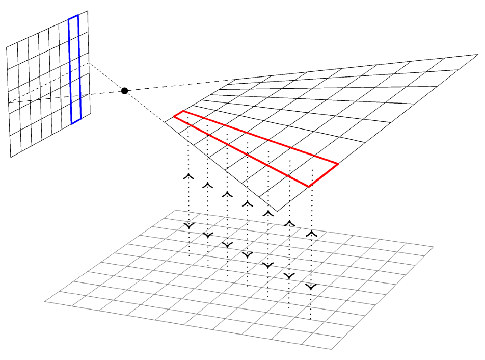
In this section, we present a camera-lidar fusion method that bypasses monocular depth estimation altogether and instead fuses camera and lidar features in bird’s-eye-view using a simple transformer [48]. A naive application of the transformer architecture to the problem of camera-lidar fusion is difficult, however, due to the large number of camera and lidar features and the quadratic nature of attention. As shown in [44], it is possible to use the geometry of the problem to drastically restrict the scope of the attention when projecting camera features in BEV, since camera features should only contribute to locations along their corresponding rays. We adapt this idea to the case of camera-lidar fusion and introduce a simple fusion method that uses cross-attention between columns in the camera plane and polar rays in the lidar BEV grid. Instead of predicting monocular depth, the cross-attention learns which camera features are the most salient given context provided by the lidar features along its ray.

With the exception of the projection of the camera features in BEV, our model shares a similar overall architecture to methods based on the Lift-Splat paradigm [33, 28, 14] and is depicted on Fig. 3 left. It consists of the following modules: the camera and lidar backbones which produce features for each modality independently, a projection and fusion module that embeds the camera features into BEV and fuses them with the lidar, and finally a detection head. When considering object detection, the final output of the model is the property of objects in the scene represented as 3D bounding boxes with position, dimension, orientation, velocity and classification information. In what follows we explain in detail the architecture of our projection and fusion modules.

Projected horizon

For each camera, we consider the horizontal line passing through the centre of the image and the plane corresponding to its projection in 3D. We call this plane the projected horizon of the camera. It can easily be described using homogeneous coordinates as the set of points $\mathbf{x}\in\mathbb{R}^{4}$ for which there exists a $u\in\mathbb{R}$ such that

$$\mathbf{C}\mathbf{x}\sim(u,h/2,1),$$ (4)

where $\mathbf{C}$ is the $3\times 4$ camera projection matrix (intrinsic and extrinsic), and $h$ is the height of the image. Note that this plane is not in general parallel to the BEV grid, its relative orientation being defined by the camera’s extrinsic parameters. We define a regular grid on the projected horizon that is aligned with the 2D grid of features in the image plane by tracing out rays from the intersection of the horizontal line with the edges of the feature columns in the image plane, and then separating these rays into a set of predetermined depth bins (similarly to [28]). Features on this grid can be represented by a matrix $G\in\mathbb{R}^{N_{D}\times W}$, where each row corresponds to a specific column in the camera feature map $F^{\text{cam}}\in\mathbb{R}^{H\times W\times C}$. The geometry of the projected horizon can be seen in Fig. 3 (left, inset).

Correspondence between projected horizons and BEV grid

We can easily define a correspondence between points on the projected horizon and points on the BEV plane by projecting them along the z-direction in 3D space. As cameras are in general tilted with respect to the ground, this correspondence depends on each camera’s extrinsic parameters. We transfer lidar features from the BEV grid to a camera’s projected horizon through bi-linear sampling of the BEV grid at the locations of the down-projected cell-centers of the projected horizon. We call this process “lifting” and denote it as $\text{Lift}_{i}$ for the projected horizon of camera $i$. Similarly, features can be transferred in the opposite direction, from projected horizon to BEV grid, by bi-linearly sampling the projected horizon at the locations of the projected cell-centers of the BEV grid. We denote this operation as $\text{Splat}_{i}$, similarly to [38, 33, 28].

Lift-Attend-Splat

Our projection module is depicted in Fig. 3 (right) and can be broken down into three simple steps: (i) we first lift the BEV lidar features $B^{\text{lid}}$ onto the projected horizon of camera $i$, producing “lifted” lidar features $\tilde{B}^{\text{lid}}_{i}$, (ii) we then let the “lifted” lidar features attend to the camera features in the corresponding column using a simple transformer encoder-decoder, producing fused features $\tilde{B}^{\text{fus}}_{i}$ on the projected horizon, and finally (iii) we splat these features back onto the BEV grid to produce $B^{\text{fus}}_{i}$. During the attend step, the camera features in each column are encoded by a transformer encoder $E$ and passed as keys and values to a transformer decoder $D$ which uses the frustum lidar features as queries. The result of these three steps can be written as

$$B^{\text{fus}}_{i}=\text{Splat}_{i}\left(D\left(\text{Lift}_{i}\left(B^{\text{lid}}\right),E\left(F_{i}^{\text{cam}}\right)\right)\right),$$ (5)

where $\text{Lift}_{i}$ and $\text{Splat}_{i}$ project the BEV features onto the projected horizon of camera $i$ (and vice versa) as described above. Finally, we apply a simple fusion module where we sum the projected features from different cameras together, concatenate them with the lidar features and apply a convolutional block to obtain the final features in BEV. This simple architecture allows the camera features to be projected from the image plane onto the BEV grid without requiring monocular depth estimation. We use a single set of column-frustum transformer weights which are shared across all column-frustum pairs and cameras. For simplicity, we use here a single transformer encoder and decoder but show that increasing the number of such blocks can be beneficial in Sec. 5.4.

Attention vs depth prediction

It is worth discussing how our approach differs from predicting monocular depth directly. When using monocular depth, each feature in the camera feature map is projected into BEV at multiple locations weighted by a normalised depth distribution. This normalisation limits each feature to be projected either into a single location or smeared with lower intensity across multiple depths. However, in our approach, the attention between camera and lidar is such that the same camera feature can contribute fully to multiple locations in the BEV grid. This is possible because attention is normalised over keys, which correspond to different heights in the camera feature map, rather than queries, which correspond to different distances along the ray. Furthermore, our model has access to lidar features in BEV when choosing where to project camera features, which gives it greater flexibility.

5 Experiments

We measure the effectiveness of our approach against recent camera-lidar fusion methods that use the Lift-Splat paradigm [28, 33]. In all of our experiments, we concentrate on 3D object detection using the nuScenes dataset [2], which is a large-scale dataset for autonomous driving. We use the nuScenes detection score (NDS) and mean average precision (mAP) as evaluation metrics. We do not consider the extension of [28, 33] presented in [14] as it introduces two supplementary dense depth supervision losses on the camera path to significantly boost the performance of the underlying methods. In this work, we use solely the 3D object detection losses present in [1, 28, 33] and leave applying the framework of [14] to our method for future work.

Overall architecture

We use Dual-Swin-Tiny [27] with a feature pyramid network [29] and VoxelNet [65] as our camera and lidar encoders respectively. For our object detection head, we use the transformer-decoder-based module from TransFusion-L [1]. We use our Lift-Attend-Splat method, described in Sec. 4, to project camera features into BEV space. We then fuse camera and lidar features using simple concatenation and convolution. Following [33] the RPN part of VoxelNet is applied to the merged feature. We ablate alternative choices for the fusion architecture in Sec. 5.4.

Implementation details

We use an image resolution of 800x448 for inputs to the camera encoder, which is downsampled 8x by the camera encoder into per-camera feature maps of shape 100x56. For VoxelNet, we follow the settings of [28]. During training, we set a maximum of 90k non-empty voxels which we increase to 180k during inference. We use a lidar BEV grid centred around the ego with dimensions $108\text{m}\times 108\text{m}$ and 0.075m cell size. This is downsampled 8x by the lidar encoder to the $180\times 180$ grid into which the camera features are projected. We construct the intermediate projected horizon with 143 uniformly spaced depth bins ranging from 1m to 72m. For the projection of camera features into BEV, we use the original transformer [48] as our encoder-decoder architecture, with one encoder layer, one decoder layer, $d_{\text{model}}=256$ and $d_{\text{ff}}=512$. We replace the ReLU [36] activation function with GeLU [13], use learnable position embeddings [10] in place of sinusoidal encodings and normalise features before each sublayer [56]. We tie the parameters in each of the 8 heads of our attention blocks. For the object detection head, we use 200 and 300 queries during training and inference respectively.

Training details

Our lidar backbone is pretrained on 8 GPUs with batch-size of 1/GPU following the schedule presented in [1], with CBGS [66] and copy-paste augmentation [58]. We initialise the camera backbone with weights pretrained on nuImages [2]. We freeze the lidar backbone and train the camera backbone, projection, fusion and detection head together for 20 epochs using 8 GPUs with batch-size of 4/GPU. We use the AdamW optimiser [34] with a maximum learning rate of $5\times 10^{-5}$ for the camera backbone and $1\times 10^{-3}$ for all other components. We apply the following augmentations: random mirror flips in Y dimensions, affine transformations (rotations and scale), and camera-lidar copy-paste augmentations [50].

5.1 3D object detection

We present results for the task of 3D object detection on Tab. 1. Compared to baselines based on the Lift-Splat projection [28, 33], our method shows improvements both on the validation and test splits of the nuScenes dataset. In particular, we show substantial improvements in both mAP ($+1.1$) and NDS ($+0.4$) on the test split. Since the lidar backbone is frozen and similar in all approaches, this shows that our model is better able to leverage camera features. Per-class object detection results as well as comparison to other methods can be found in Tab. S2 and Sec. B.1.

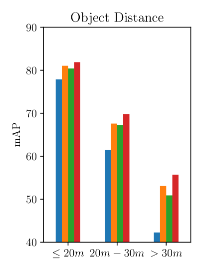
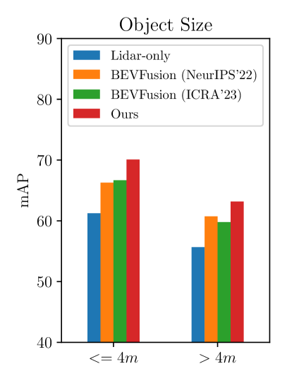
We can analyse further the performance of our model by clustering objects together depending on their distances from the ego and on their sizes, see Fig. 4. We see that the bulk of the improvements comes from objects located at large distances and of small sizes. These are situations for which monocular depth estimation is particularly difficult which could explain why our model fares better in these cases. Note that even though far-away and small objects contain less lidar points, our model is still able to leverage camera features effectively even though the context given by the lidar is weaker.

Finally, we show results that use test-time-augmentations (TTA) and model ensembling at the bottom of Tab. 1. We perform TTA over a combination of mirror and rotation augmentations and ensemble models with cell resolutions of 0.05m, 0.075m and 0.10m. We first apply TTA at each cell resolution and then merge the resulting boxes using Weighted Boxes Fusion (WBF) [47]. Unsurprisingly, our method shows excellent scaling with respect to these techniques and outperforms BEVFusion [33] on the nuScenes validation set. More details can be found in Sec. B.3.

	val.		test
	mAP	NDS	mAP	NDS
BEVFusion [33]	68.5	71.4	70.2	72.9
BEVFusion [28]	69.6	72.1	71.3	73.3
Ours	71.2	72.7	71.5	73.6
Ours w/ TFA	72.1	73.8	-	-
BEVFusion‡ [33]	73.7	74.9	75.0	76.1
Ours‡	74.6	75.1	-	-
Ours w/ TFA‡	75.7	76.0	75.5	74.9

Table 1: Our method compared to LiftSplat-based camera-lidar fusion baselines on the validation and test splits of the nuScenes dataset. TFA: Temporal Feature Aggregation. ^‡ denotes test-time augmentations and model ensembling.

Figure 4: Object detection performance measured using mAP for objects at different distances from the ego and of different sizes. Our model consistently outperforms baselines based on Lift-Splat, especially at large distances and for small objects.

5.2 Qualitative analysis

Ours

(a)

BEVFusion [33]

(b)

Ours

BEVFusion [33]

(c)

Camera+lidar

Camera only

Figure 5: (a, b) Visualisation of where camera features of ground-truth objects are projected onto the BEV grid for our method compared to BEVFusion [33]. We observe that our method is able to place camera features around objects more narrowly than BEVFusion, which is based on monocular depth estimation. (c) Comparison of object saliency maps for models trained with camera only (top) and camera and lidar (bottom). When trained with both camera and lidar, our model selects camera features in an area that is different than when trained with camera only, while [33] behaves similarly in both settings. Saliency maps and original images show the corresponding ground-truth box for context.

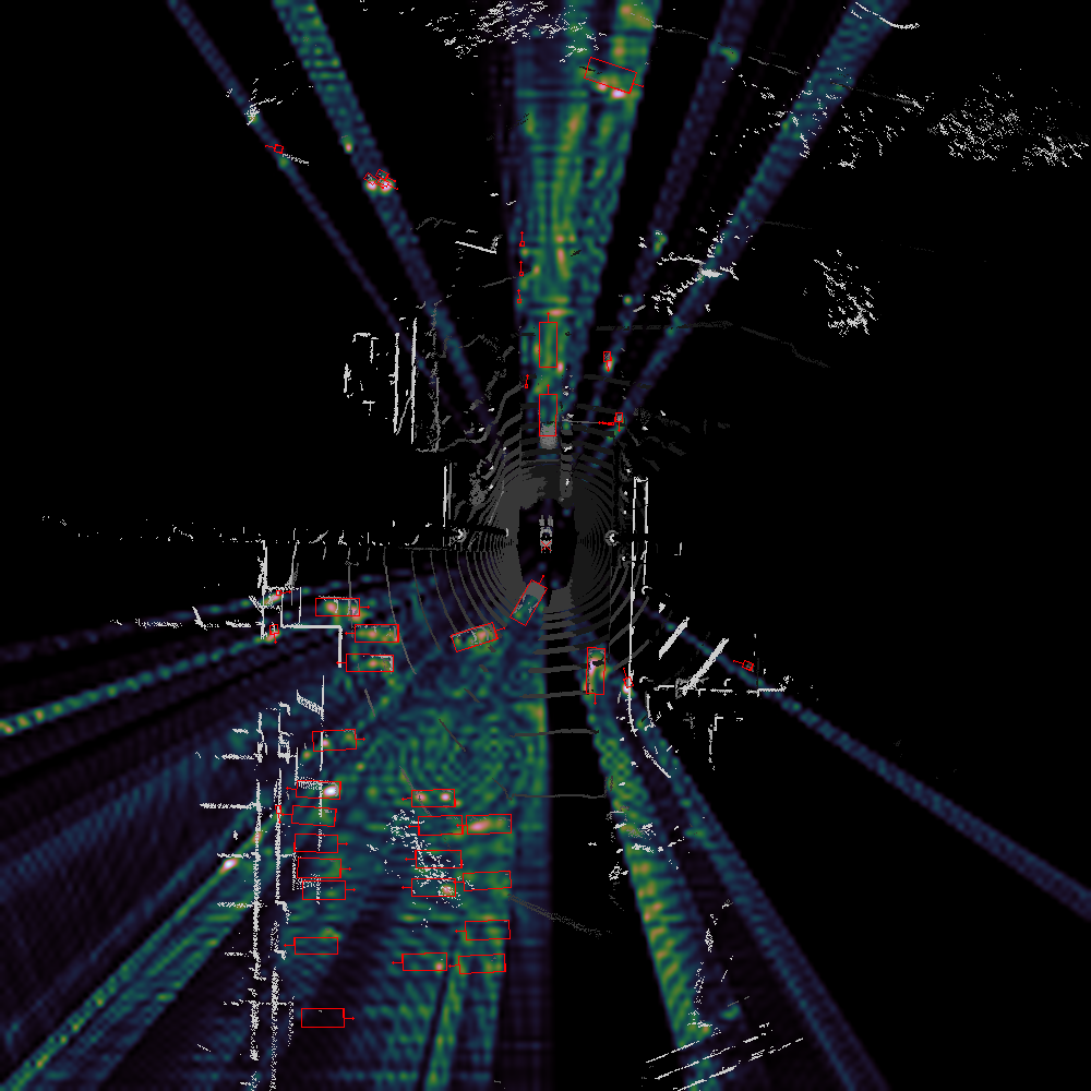
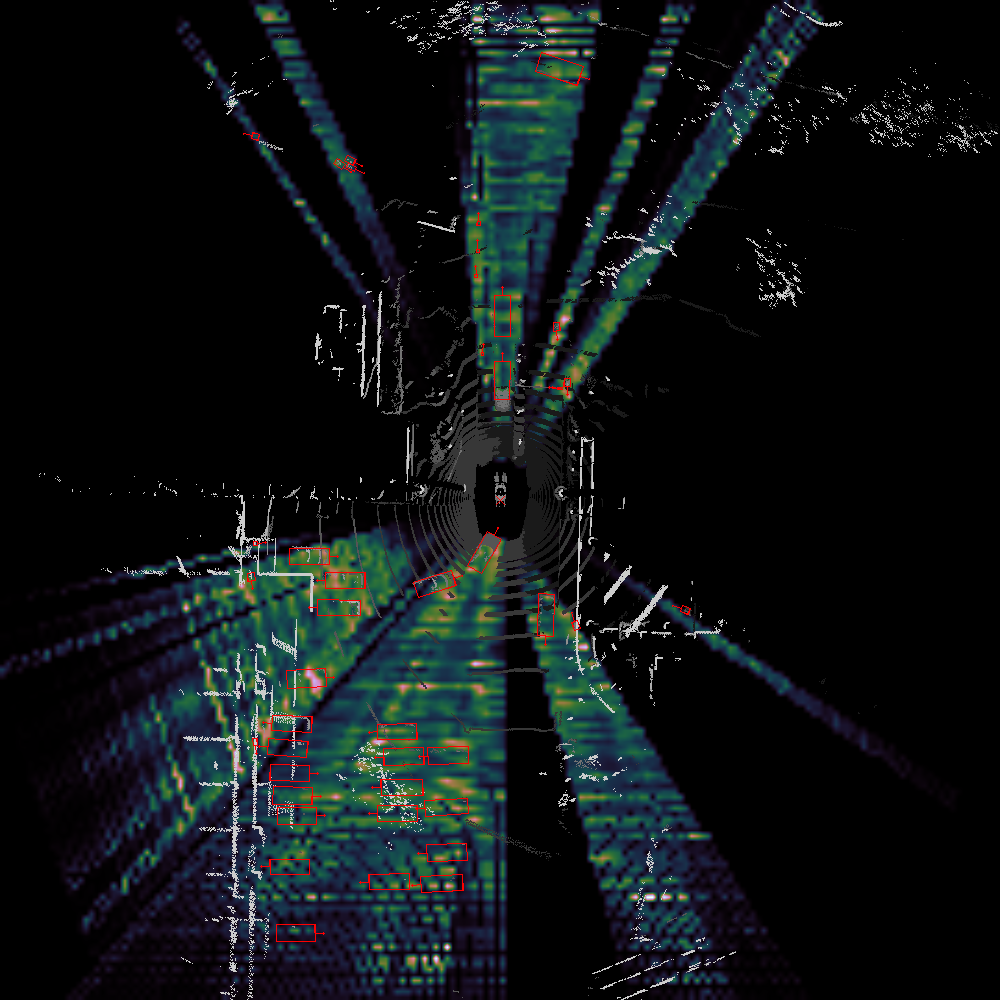
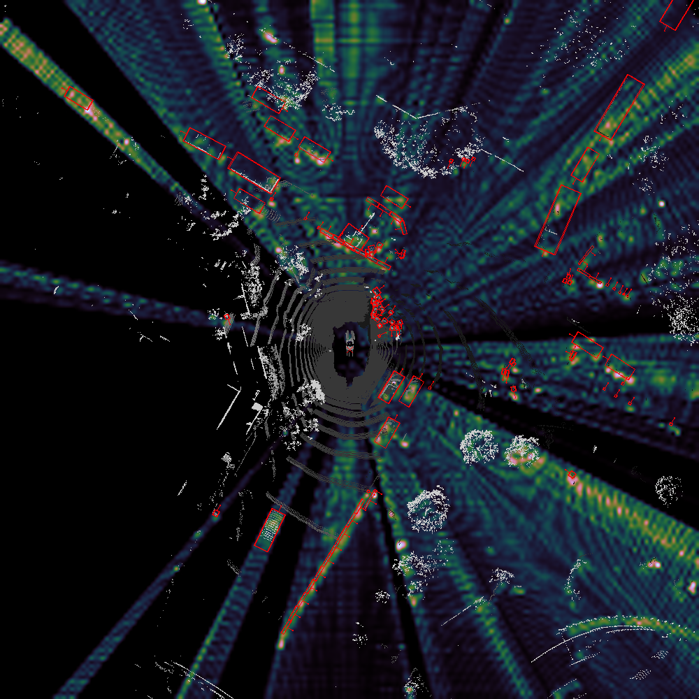
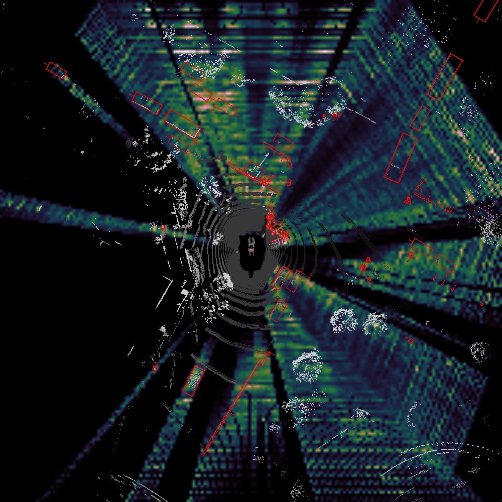
We visualise where camera features are projected onto the BEV grid and compare our method to BEVFusion [33]. For our method, we examine the attention map of the final cross-attention block in the transformer, averaged over all attention heads. For BEVFusion, we use the the monocular depth estimate to establish the strength of correspondence between positions in camera and BEV space. We consider only the pixels corresponding to ground-truth objects when calculating the total weight of projected camera features in BEV, see Sec. B.2 for details. As can be seen in Fig. 5(a) (left), our method places camera features predominantly in regions where ground-truth bounding boxes are present. This indicates that it can effectively leverage the lidar point cloud as a context in order to project camera features at the relevant location in BEV. Compared to BEVFusion shown in Fig. 5(b), the distribution of features appears more narrowly localised and stronger around objects. This could be due to the fact our projection mechanism does not require the weights of the camera features to be normalised along their ray, giving our model more flexibility to place features at the desired location. It is interesting to note that even though our method also projects camera features outside of ground-truth boxes in BEV, the strength of the activation in these regions is suppressed by the fusion module, see Fig. S4. This is consistent with our findings in Sec. 3, where we showed that the latter part of the model is able to effectively suppress camera features at the wrong location. More examples can be found in Sec. B.2.

We further explore which pixels in the camera images are most attended to using saliency maps [46]. These are derived by computing the gradient of the maximum class logit with respect to a camera image $I_{j}$, given object query index $i$ and probabilities $z$, as:

$$\left.\frac{\partial z_{i,\hat{c}}}{\partial I}\right|_{I_{j}}\text{where }\hat{c}=\arg\max_{c}z_{i,c}.$$ (6)

They allow us to visualise the contribution of individual pixels to the final prediction for a selected object, see Fig. S2 (right). Interestingly, we observe that when trained with both camera and lidar, our model tends to select camera features at different locations than when trained with cameras only. In the absence of lidar, our method selects camera features across the entirety of the object, while in the presence of both lidar and cameras, the model selects camera features mainly from the upper part of the object. We observe that this pattern is mostly prevalent for objects close to the ego which are well-represented by lidar point clouds but fades away for far-away objects or objects with few lidar points such as pedestrians, see Fig. S2 for more examples. We hypothesise that our projection architecture enables the model to select camera features that complement best the information encoded in lidar, resulting in differing attention patterns between camera-only and fusion settings. This pattern is less present in BEVFusion [33], which attends to the broader neighbourhood of pixels surrounding the selected object in both cases.

5.3 Temporal feature aggregation

Because our method fuses camera and lidar features onto a BEV grid, we can easily leverage past information using temporal feature aggregation (TFA). To achieve this, we implement the simple autoregressive procedure of VideoBEV [12] but aggregate the fused BEV features $B^{\text{fus.}}$ instead of the camera features. Our method is as follows: (i) save the fused BEV features from the previous timestep, (ii) apply ego motion compensation to align these features with the current timestep, using bilinear sampling to construct the new feature grid, (iii) concatenate these features with the fused BEV features of the current timestep and merge them using a simple $3\times 3$ convolutional block.

We train TFA models on sequences of 3 frames for 10 epochs starting from a pretrained object detection head, lidar and camera backbones (from our single frame model). During training, the lidar and camera backbones are kept frozen. For inference, we accumulate BEV features for the entire length of a run, yielding detections at each time step. Table 1 shows that temporal feature aggregation boosts object detection performance significantly, both without and with TTA and model ensembling.

5.4 Ablation experiments

	mAP	NDS
Fusion module:
Cat+Conv	70.43	71.9
Gated sigmoid [28]	70.12	71.9
Add	70.32	72.1
Number of decoder blocks∗:
1 block	70.29	71.9
2 blocks	70.40	72.0
4 blocks	70.49	71.9
Number of frames in TFA:
1 frame (no TFA)	71.2	72.8
2 frames	72.1	73.3
3 frames	72.1	73.8

Table 2: Impact of various modifications of our model on 3D object detection performance: (i) feature fusion module, (ii) number of transformer decoder blocks in the “Attend” stage, (iii) number of frames in Temporal Feature Aggregation (TFA). ^∗ indicates frozen camera backbone.

We ablate some design choices for our method and show their impact on object detection performance on Tab. 2. For all the ablation experiments, we use a simpler training schedule with 10 epochs, batch accumulation instead of full batch training and no camera augmentations. We first analyse the impact of different implementations of the fusion module: we compare a simple skip connection (add), a small concatenation and convolution layer (Cat+Conv as in [33]) and a gated sigmoid block [28]. We find all of them to perform very similarly, with Cat+Conv performing slightly beter with respect to mAP, contrary to findings of [28]. We also ablate the number of transformer decoder blocks in the “Attend” stage of our projection and show that increasing their number does lead to small improvement in mAP. This suggests that our method can scale up with increased compute but we use a single decoder block in our experiments as it provides good balance between quality and performance. Finally, we also see good improvement in detection score when increasing number of frames in Temporal Feature Aggregation during training.

6 Conclusion

In this work, we have analysed the role of monocular depth prediction in recent state-of-the-art camera-lidar fusion methods and showed that, surprisingly, improvements in depth estimation did not lead to better object detection performance. Strikingly, we also showed that removing depth estimation altogether did not worsen performance significantly. This led us to hypothesise that relying on monocular depth estimation could be an unnecessary architectural bottleneck when fusing camera and lidar, and prompted us to introduce a novel fusion method that directly combines camera and lidar features using a simple attention mechanism. Compared to projecting camera features using monocular depth, our method allows camera features to contribute to multiple locations in BEV space and gives our model greater flexibility to select complementary camera and lidar features. Finally, we validated the effectiveness of our method on the nuScenes dataset and showed that it improves object detection performance over baselines based on monocular depth estimation and showcased the role of attention as a key contributor to these improvements. We hope that our work will motivate discussions around the role of monocular depth prediction in camera-lidar fusion and motivate further developments in multi-modal perception more generally.

Supplementary Material

A Monocular depth in the “LiftSplat” paradigm

A.1 Computation of ground truth depth from lidar

For each camera image we compute the ground depth map $D^{\text{gt}}\in\mathbb{R}^{H\times W}$ by projecting the 3D lidar point cloud onto the image plane and binning each point within the pixels of the camera feature map. For non-empty cells, we follow [24] and choose the depth to be the minimum distance (from the camera plane) of all the points in the cell, leaving the depth unspecified for empty cells and those for which the minimum yields a depth value which is outside the range of the model’s depth bins. This depth map is suitable for visualisation and depth metric evaluation, but for depth supervision it is necessary to calculate the one-hot encoding of $D^{\text{gt}}$ according to buckets defined by the model’s depth bins $d\in\mathbb{R}^{N_{D}}$.

A.2 Visualisation of depth maps

We generate the monocular depth maps shown in Fig. 1 by calculating the weighted average of the model’s depth bins $d$ with the predicted depth distribution $D^{\text{pred}}\in\mathbb{R}^{N_{D}\times H\times W}$

$$D^{\text{mean}}_{h,w}=\sum^{N_{D}}_{n}{d_{n}D^{\text{pred}}_{n,h,w}}.$$ (7)

This depth map is constrained by construction to $[\text{min}(d),\text{max}(d)]$ and we map this range onto the Turbo colour map [35] for visualisation.

The lidar depth map $D^{\text{gt}}$ is similarly colourised, except for cells where the depth is unspecified as described above (see  Fig. S1, top-right) which are coloured grey.

A.3 Supervision of predicted depth using lidar

We perform all of our experiments using the method presented in [33] and use the original repository. We use the vanilla Lift-Splat transform implemented in the class LSSTransform with default parameters provided in the original work. We supervise the depth classifier by introducing the following loss alongside the original detection losses,

$$L_{\text{depth}}=-\frac{1}{N}\sum_{n}^{N}\text{log}(D_{n}\cdot 1_{n}),$$ (8)

which is a cross-entropy loss between the lidar depth distribution and predicted depth distribution, taken over all cells for which the lidar depth is available. $D_{n}\in\mathbb{R}^{N_{D}}$ is the normalised predicted depth distribution from the LiftSplat model for the $n$th cell, $1_{n}$ is the one-hot encoded lidar depth distribution for the $n$th cell. The model is trained end-to-end with all components unfrozen as in [33] and hyper-parameter $\lambda$ controlling the strength of the depth supervision loss with respect to the detection losses.

We also experiment with pretraining the depth estimation module within LiftSplat. First, we train the camera stream in [33] supervising only the depth distribution with the whole camera pipeline unfrozen. Following this pretraining, we add the lidar components and train the full model end-to-end as in [33], with no depth supervision ($\lambda=0$) and all modules unfrozen.

Loss Weight	mAP	mode					mean
		Relative		RMSE		Frac. 125	Relative		RMSE		Frac. 125
		Abs.	Sq.	Linear	Log		Abs.	Sq.	Linear	Log
BEVFusion [33]	68.5	2.95	133.76	25.95	1.87	0.97	2.75	61.31	17.40	1.30	0.88
$\lambda=0$	68.4	3.69	176.09	30.22	1.90	0.96	2.83	68.73	18.54	1.34	0.87
0.001	68.1	1.79	65.63	20.16	1.77	0.94	3.14	79.87	19.91	1.39	0.88
0.01	68.0	0.61	11.78	11.54	1.03	0.63	0.76	10.30	8.09	0.68	0.61
0.1	68.1	0.38	5.53	9.28	0.77	0.41	0.43	4.97	6.47	0.46	0.37
1	68.1	0.21	2.48	5.78	0.37	0.20	0.22	2.23	4.77	0.33	0.19
5	66.6	0.19	2.01	4.77	0.33	0.17	0.19	1.95	4.53	0.32	0.17
100	64.6	0.16	1.15	4.64	0.33	0.17	0.16	1.12	4.55	0.32	0.17
Pretrained	67.4	0.54	8.10	9.95	0.86	0.61	0.64	7.91	7.87	0.66	0.57
Lidar	68.4	0.04	0.01	0.29	0.05	0.00	0.04	0.01	0.29	0.05	0.00
No depth	68.5	–	–	–	–	–	–	–	–	–	–

Table S1: Extended analysis of the monocular depth quality provided by different variations of the “LiftSplat” camera feature projection, see Sec. A.4.

A.4 Extended depth quality results

We evaluate the performance of the depth classifier using five of the metrics proposed in [9]: root mean squared error (RMSE), root mean squared logarithmic error (RMSLE), mean absolute relative error (Abs. Rel.), mean squared relative error (Sq. Rel.) and fraction outside 125% (Frac. 125). We show all the metrics for 2 different methods of translating the classification output into a depth map: “mode” — in which we use the bin with maximum probability, and “mean” — where the predicted depth is the weighted average of all the bins. We take the average of these quantities over all predictions made by the depth classifier for which we have ground truth to compute the metrics. Camera feature cells for which lidar depth is unspecified are ignored. We compare BEVFusion and four different variants: adding depth supervision using Eq. 2 with various weights $\lambda$, using lidar depth maps instead of monocular depth estimation (lidar), using a pretrained and frozen depth classifier (pretrained), and finally removing depth estimation altogether by projecting camera features at all depths uniformly using Eq. 3 (no depth). Quantitative results can be seen in Tab. S1 and qualitative comparisons in Fig. S1.

B Detailed experimental results

Camera

Lidar

End-to-end [33]

Supervised $\lambda=0$

Supervised $\lambda=0.001$

Supervised $\lambda=0.01$

Supervised $\lambda=0.1$

Supervised $\lambda=1$

Supervised $\lambda=5$

Supervised $\lambda=100$

Figure S1: Depth maps obtained after different levels of depth supervision on an example from the nuScenes val set.

B.1 3D object detection

Model	barrier	bicycle	bus	car	CV	MC	ped	TC	trailer	truck	mAP	NDS
Ours	74.1	70.0	81.3	90.3	33.8	80.8	89.3	79.7	44.0	68.2	71.2	72.7
BEVFusion[28]	73.5	67.5	77.7	89.1	30.9	79.0	89.4	79.3	42.6	66.7	69.6	72.1
DeepInteraction[61]	78.1	52.9	68.3	87.1	33.1	73.6	88.4	86.7	60.8	60.0	69.9	72.6
Ours‡	77.5	75.2	82.3	91.2	40.0	85.6	90.6	80.2	50.1	72.2	74.6	75.1
Ours w/ TFA	74.4	72.4	81.6	90.8	33.7	82.5	89.8	79.6	45.8	70.1	72.1	73.8
Ours‡ w/ TFA	78.6	78.2	84.3	91.6	39.9	87.5	91.4	80.7	51.2	73.3	75.7	76.0
Ours	78.0	54.9	72.1	89.0	38.9	75.3	90.3	87.0	65.3	64.2	71.5	73.6
Ours‡ w/ TFA	79.7	65.2	75.2	90.3	43.5	82.8	92.0	87.1	70.1	68.9	75.5	74.9
BEVFusion[28]	78.3	56.5	72.0	88.5	38.1	75.2	90.0	86.5	64.7	63.1	71.3	73.3
DeepInteraction[61]	80.4	54.5	70.8	87.9	37.5	75.4	91.7	87.2	63.8	60.2	70.8	73.4

Table S2: Per-class object detection scores on the nuScenes validation set (top) and test set (bottom). TFA: Temporal Feature Aggregation. ^‡ indicates ensembling + TTA.

In  Tab. S2 we present per-class detection scores and compare our model to other state-of-the-art models on the validation and test splits of the nuScenes dataset. Our method outperforms baselines based on the LiftSplat paradigm. We are additionally showing how test-time-augmentations and temporal feature aggregation further improves these results.

B.2 Detailed qualitative results

Ours

BEVFusion [33]

(a)

Ours

BEVFusion [33]

(b)

Cam+lidar

Cam-only

Ours

BEVFusion [33]

(c)

Ours

BEVFusion [33]

(d)

Cam+lidar

Cam-only

Figure S2: (a) Similar attention pattern as highlighted in the main text for a close object which is well-represented by the lidar point cloud. (b) For the same object, but at a later frame when the car moved further away from the ego, our model attends to the same area when trained with camera and lidar as when trained with camera only (left). (c) For an occluded object, whose representation in the lidar point cloud is weaker, our model attends to the entire unoccluded area in both settings. BEVFusion [33] appears to consistently attend to a larger neighbourhood of pixels. (d) The pedestrian, who is not well-represented by the lidar point cloud, is fully attended by our model in the presence of lidar and camera.

Scene

(a)

Mask

(b)

Figure S3: (a) Camera image $I_{i}$ with annotations highlighted in white and our model’s predictions, in colour. (b) Binary image $\text{Mask}^{(i)}$ created by in-painting the annotations.

Before fusion module

(a)

After fusion module

(b)

Figure S4: Activations in BEV space derived by summing up feature maps along the channel dimension. (a) uses the channel-wise concatenation of lidar and projected camera features. (b) uses the output of the fusion module, demonstrating its efficacy in suppressing background activations.

Ours

(a)

BEVFusion [33]

(b)

Ours

(c)

BEVFusion [33]

(d)

Figure S5: Additional examples showcasing the weight of projected camera features onto the BEV space. All examples presented in the analysis are from the validation set.

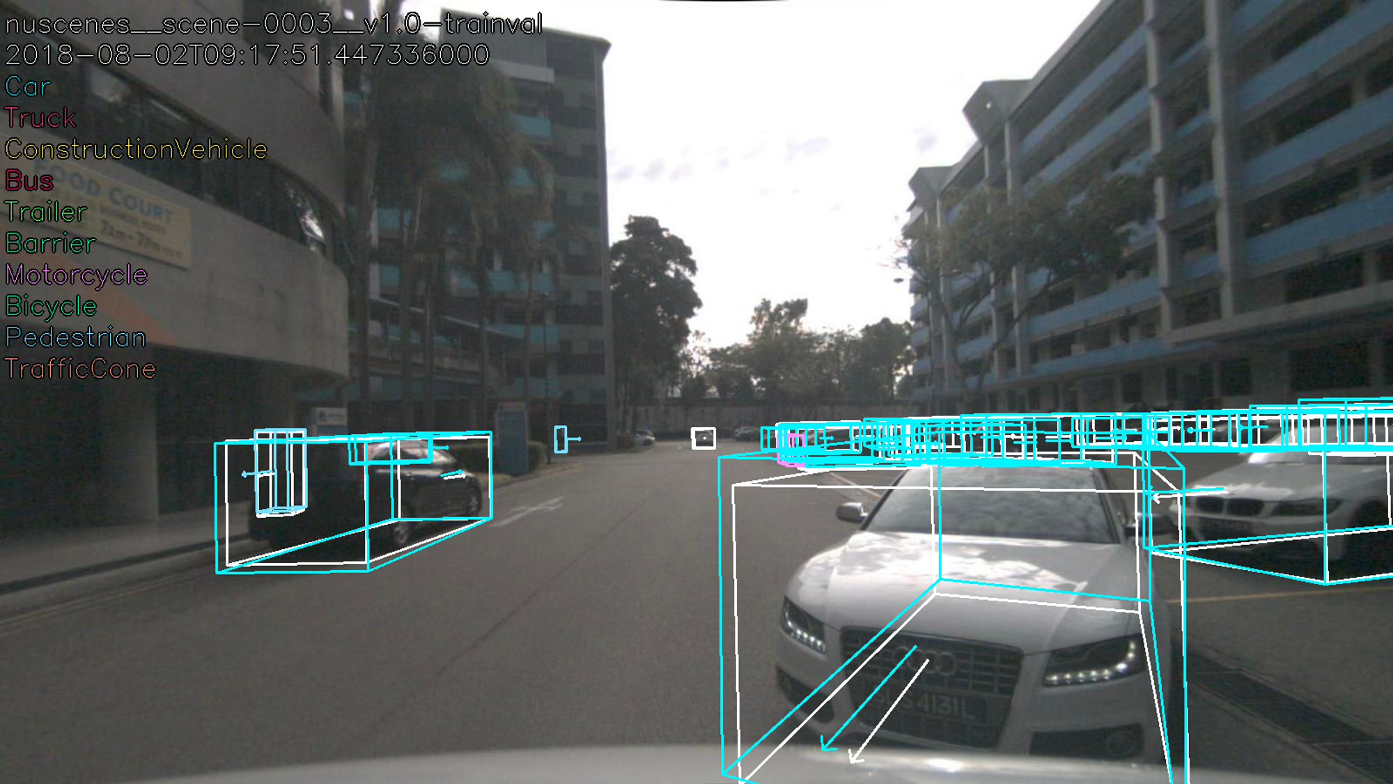
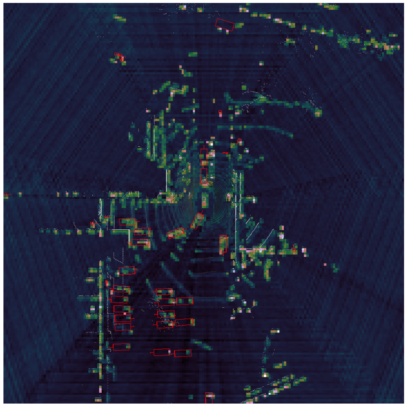
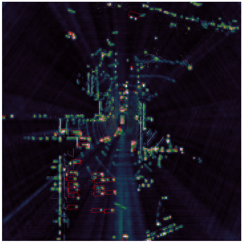
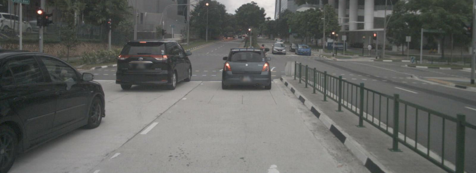
To obtain Figure 5(a) for our method, we first compute the full camera-to-BEV attention map $\text{Attn}^{(\text{cam}_{i}\rightarrow\text{bev})}\in\mathbb{R}^{H\times W\times N\times M}$. To do so, we extract the attention map of the last transformer decoder block by averaging over all heads, $\text{Attn}^{(\text{cam}_{i}\rightarrow\text{frustum})}\in\mathbb{R}^{H\times W\times D\times W^{\prime}}$, where $(D\times W^{\prime})$ corresponds to the frustum dimension. We construct $\text{Attn}^{(\text{cam}_{i}\rightarrow\text{bev})}$ by scattering the frustum attention values onto the BEV grid. Given camera image $I_{i}$, we then create $\text{Mask}^{(i)}\in\{0,1\}^{H\times W}$ by in-paint drawing the annotations, see Fig. S3, and obtain the BEV attention $\text{Attn}^{(\text{bev})}\in\mathbb{R}^{N\times M}$ shown on Figure 5(a) by projecting these camera features onto the BEV grid:

$$\text{Attn}^{(\text{bev})}=\max_{i,h,w}\text{Attn}_{h,w}^{(\text{cam}_{i}\rightarrow\text{bev})}\cdot\text{Mask}_{h,w}^{(i)}.$$ (9)

To obtain a similar visualisation for the “LiftSplat” projection, see Figure 5(b), we adjust the implementation of [33] but use the same model weights. Firstly, we replace the feature map of image $I_{i}$ with $\text{Mask}^{(i)}$ and use that as input to the projection. This binary mask is “lifted” onto a 3D point cloud using the normalised depth classification weights $D_{i}$ for which we clipped the first 5 and last 5 depth bins. $\text{Mask}^{(i)}$ thus acts as an indicator function and $D_{i}$ specifies the strength of correspondence between pixels and the 3D point cloud $P\in\mathbb{R}^{H\times W\times N_{D}\times 3}$. Secondly, during “splatting”, we project points onto the z = 0 plane and pool them using max. This operation ensures that the weight of attention for large objects in the final visualisation does not overpower that of smaller objects.

B.3 Ensemble and test-time augmentations

For test-time-augmentation (TTA) and model ensembling, we use WBF [47] based on L2 distance metric per object category to decide which of the boxes to fuse. We first carry out TTA (using mirror and rotation augmentations) with WBF for each cell resolution, and then apply another WBF on the outputs from TTA of each model to get the final detections which we use for evaluations. For rotation augmentation, we use (-12.5, -6.25, 0, 6.25, 12.5) degrees.

References

- Bai et al. [2022] Xuyang Bai, Zeyu Hu, Xinge Zhu, Qingqiu Huang, Yilun Chen, Hongbo Fu, and Chiew-Lan Tai. Transfusion: Robust lidar-camera fusion for 3d object detection with transformers. In Proceedings of the IEEE/CVF conference on computer vision and pattern recognition, pages 1090–1099, 2022.
- Caesar et al. [2020] Holger Caesar, Varun Bankiti, Alex H Lang, Sourabh Vora, Venice Erin Liong, Qiang Xu, Anush Krishnan, Yu Pan, Giancarlo Baldan, and Oscar Beijbom. nuscenes: A multimodal dataset for autonomous driving. In Proceedings of the IEEE/CVF conference on computer vision and pattern recognition, pages 11621–11631, 2020.
- Chen et al. [2016] Xiaozhi Chen, Kaustav Kundu, Ziyu Zhang, Huimin Ma, Sanja Fidler, and Raquel Urtasun. Monocular 3d object detection for autonomous driving. In 2016 IEEE Conference on Computer Vision and Pattern Recognition (CVPR), pages 2147–2156, 2016.
- Chen et al. [2017] Xiaozhi Chen, Huimin Ma, Ji Wan, Bo Li, and Tian Xia. Multi-view 3d object detection network for autonomous driving. In Proceedings of the IEEE conference on Computer Vision and Pattern Recognition, pages 1907–1915, 2017.
- Chen et al. [2022a] Yukang Chen, Yanwei Li, Xiangyu Zhang, Jian Sun, and Jiaya Jia. Focal sparse convolutional networks for 3d object detection. In Proceedings of the IEEE/CVF Conference on Computer Vision and Pattern Recognition, pages 5428–5437, 2022a.
- Chen et al. [2022b] Zehui Chen, Zhenyu Li, Shiquan Zhang, Liangji Fang, Qinghong Jiang, Feng Zhao, Bolei Zhou, and Hang Zhao. Autoalign: pixel-instance feature aggregation for multi-modal 3d object detection. arXiv preprint arXiv:2201.06493, 2022b.
- Chong et al. [2022] Zhiyu Chong, Xinzhu Ma, Hong Zhang, Yuxin Yue, Haojie Li, Zhihui Wang, and Wanli Ouyang. Monodistill: Learning spatial features for monocular 3d object detection. arXiv preprint arXiv:2201.10830, 2022.
- Drews et al. [2022] Florian Drews, Di Feng, Florian Faion, Lars Rosenbaum, Michael Ulrich, and Claudius Gläser. Deepfusion: A robust and modular 3d object detector for lidars, cameras and radars. In 2022 IEEE/RSJ International Conference on Intelligent Robots and Systems (IROS), pages 560–567. IEEE, 2022.
- Eigen et al. [2014] David Eigen, Christian Puhrsch, and Rob Fergus. Depth map prediction from a single image using a multi-scale deep network. In Advances in Neural Information Processing Systems. Curran Associates, Inc., 2014.
- Gehring et al. [2017] Jonas Gehring, Michael Auli, David Grangier, Denis Yarats, and Yann N Dauphin. Convolutional sequence to sequence learning. In International conference on machine learning, pages 1243–1252. PMLR, 2017.
- Guo et al. [2021] Xiaoyang Guo, Shaoshuai Shi, Xiaogang Wang, and Hongsheng Li. Liga-stereo: Learning lidar geometry aware representations for stereo-based 3d detector. In Proceedings of the IEEE/CVF International Conference on Computer Vision, pages 3153–3163, 2021.
- Han et al. [2023] Chunrui Han, Jianjian Sun, Zheng Ge, Jinrong Yang, Runpei Dong, Hongyu Zhou, Weixin Mao, Yuang Peng, and Xiangyu Zhang. Exploring recurrent long-term temporal fusion for multi-view 3d perception. arXiv preprint arXiv:2303.05970, 2023.
- Hendrycks and Gimpel [2016] Dan Hendrycks and Kevin Gimpel. Gaussian error linear units (gelus). arXiv preprint arXiv:1606.08415, 2016.
- Hu et al. [2023] Haotian Hu, Fanyi Wang, Jingwen Su, Yaonong Wang, Laifeng Hu, Weiye Fang, Jingwei Xu, and Zhiwang Zhang. Ea-lss: Edge-aware lift-splat-shot framework for 3d bev object detection, 2023.
- Huang et al. [2022] Dihe Huang, Ying Chen, Yikang Ding, Jinli Liao, Jianlin Liu, Kai Wu, Qiang Nie, Yong Liu, Chengjie Wang, and Zhiheng Li. Rethinking dimensionality reduction in grid-based 3d object detection. arXiv preprint arXiv:2209.09464, 2022.
- Huang et al. [2021] Junjie Huang, Guan Huang, Zheng Zhu, Yun Ye, and Dalong Du. Bevdet: High-performance multi-camera 3d object detection in bird-eye-view. arXiv preprint arXiv:2112.11790, 2021.
- Huang et al. [2020] Tengteng Huang, Zhe Liu, Xiwu Chen, and Xiang Bai. Epnet: Enhancing point features with image semantics for 3d object detection. In Computer Vision–ECCV 2020: 16th European Conference, Glasgow, UK, August 23–28, 2020, Proceedings, Part XV 16, pages 35–52. Springer, 2020.
- Jiang et al. [2023] Xiaohui Jiang, Shuailin Li, Yingfei Liu, Shihao Wang, Fan Jia, Tiancai Wang, Lijin Han, and Xiangyu Zhang. Far3d: Expanding the horizon for surround-view 3d object detection. arXiv preprint arXiv:2308.09616, 2023.
- Koh et al. [2023] Junho Koh, Junhyung Lee, Youngwoo Lee, Jaekyum Kim, and Jun Won Choi. Mgtanet: Encoding sequential lidar points using long short-term motion-guided temporal attention for 3d object detection. In Proceedings of the AAAI Conference on Artificial Intelligence, pages 1179–1187, 2023.
- Ku et al. [2018] Jason Ku, Melissa Mozifian, Jungwook Lee, Ali Harakeh, and Steven L Waslander. Joint 3d proposal generation and object detection from view aggregation. In 2018 IEEE/RSJ International Conference on Intelligent Robots and Systems (IROS), pages 1–8. IEEE, 2018.
- Ku et al. [2019] Jason Ku, Alex D Pon, and Steven L Waslander. Monocular 3d object detection leveraging accurate proposals and shape reconstruction. In Proceedings of the IEEE/CVF conference on computer vision and pattern recognition, pages 11867–11876, 2019.
- Lang et al. [2019] Alex H Lang, Sourabh Vora, Holger Caesar, Lubing Zhou, Jiong Yang, and Oscar Beijbom. Pointpillars: Fast encoders for object detection from point clouds. In Proceedings of the IEEE/CVF conference on computer vision and pattern recognition, pages 12697–12705, 2019.
- Li et al. [2022a] Yingwei Li, Adams Wei Yu, Tianjian Meng, Ben Caine, Jiquan Ngiam, Daiyi Peng, Junyang Shen, Yifeng Lu, Denny Zhou, Quoc V Le, et al. Deepfusion: Lidar-camera deep fusion for multi-modal 3d object detection. In Proceedings of the IEEE/CVF Conference on Computer Vision and Pattern Recognition, pages 17182–17191, 2022a.
- Li et al. [2023] Yinhao Li, Zheng Ge, Guanyi Yu, Jinrong Yang, Zengran Wang, Yukang Shi, Jianjian Sun, and Zeming Li. Bevdepth: Acquisition of reliable depth for multi-view 3d object detection. In Proceedings of the AAAI Conference on Artificial Intelligence, pages 1477–1485, 2023.
- Li et al. [2022b] Zhiqi Li, Wenhai Wang, Hongyang Li, Enze Xie, Chonghao Sima, Tong Lu, Yu Qiao, and Jifeng Dai. Bevformer: Learning bird’s-eye-view representation from multi-camera images via spatiotemporal transformers. In European conference on computer vision, pages 1–18. Springer, 2022b.
- Liang et al. [2018] Ming Liang, Bin Yang, Shenlong Wang, and Raquel Urtasun. Deep continuous fusion for multi-sensor 3d object detection. In Proceedings of the European conference on computer vision (ECCV), pages 641–656, 2018.
- Liang et al. [2022a] Tingting Liang, Xiaojie Chu, Yudong Liu, Yongtao Wang, Zhi Tang, Wei Chu, Jingdong Chen, and Haibin Ling. CBNet: A composite backbone network architecture for object detection. IEEE Transactions on Image Processing, 31:6893–6906, 2022a.
- Liang et al. [2022b] Tingting Liang, Hongwei Xie, Kaicheng Yu, Zhongyu Xia, Zhiwei Lin, Yongtao Wang, Tao Tang, Bing Wang, and Zhi Tang. Bevfusion: A simple and robust lidar-camera fusion framework. Advances in Neural Information Processing Systems, 35:10421–10434, 2022b.
- Lin et al. [2017] Tsung-Yi Lin, Piotr Dollár, Ross Girshick, Kaiming He, Bharath Hariharan, and Serge Belongie. Feature pyramid networks for object detection. In Proceedings of the IEEE conference on computer vision and pattern recognition, pages 2117–2125, 2017.
- Lin et al. [2022] Xuewu Lin, Tianwei Lin, Zixiang Pei, Lichao Huang, and Zhizhong Su. Sparse4d: Multi-view 3d object detection with sparse spatial-temporal fusion. arXiv preprint arXiv:2211.10581, 2022.
- Liu et al. [2022] Yingfei Liu, Tiancai Wang, Xiangyu Zhang, and Jian Sun. Petr: Position embedding transformation for multi-view 3d object detection. In European Conference on Computer Vision, pages 531–548. Springer, 2022.
- Liu et al. [2023a] Yingfei Liu, Junjie Yan, Fan Jia, Shuailin Li, Aqi Gao, Tiancai Wang, and Xiangyu Zhang. Petrv2: A unified framework for 3d perception from multi-camera images. In Proceedings of the IEEE/CVF International Conference on Computer Vision, pages 3262–3272, 2023a.
- Liu et al. [2023b] Zhijian Liu, Haotian Tang, Alexander Amini, Xinyu Yang, Huizi Mao, Daniela L Rus, and Song Han. Bevfusion: Multi-task multi-sensor fusion with unified bird’s-eye view representation. In 2023 IEEE International Conference on Robotics and Automation (ICRA), pages 2774–2781. IEEE, 2023b.
- Loshchilov and Hutter [2017] Ilya Loshchilov and Frank Hutter. Decoupled weight decay regularization. arXiv preprint arXiv:1711.05101, 2017.
- Mikhailov [2019] Anton Mikhailov. Turbo, an improved rainbow colormap for visualization. https://blog.research.google/2019/08/turbo-improved-rainbow-colormap-for.html, 2019. Accessed: 20th October 2023.
- Nair and Hinton [2010] Vinod Nair and Geoffrey E Hinton. Rectified linear units improve restricted boltzmann machines. In Proceedings of the 27th international conference on machine learning (ICML-10), pages 807–814, 2010.
- Parida et al. [2020] Kranti Parida, Neeraj Matiyali, Tanaya Guha, and Gaurav Sharma. Coordinated joint multimodal embeddings for generalized audio-visual zero-shot classification and retrieval of videos. In Proceedings of the IEEE/CVF winter conference on applications of computer vision, pages 3251–3260, 2020.
- Philion and Fidler [2020] Jonah Philion and Sanja Fidler. Lift, splat, shoot: Encoding images from arbitrary camera rigs by implicitly unprojecting to 3d. In Computer Vision–ECCV 2020: 16th European Conference, Glasgow, UK, August 23–28, 2020, Proceedings, Part XIV 16, pages 194–210. Springer, 2020.
- Piergiovanni et al. [2021] AJ Piergiovanni, Vincent Casser, Michael S Ryoo, and Anelia Angelova. 4d-net for learned multi-modal alignment. In Proceedings of the IEEE/CVF International Conference on Computer Vision, pages 15435–15445, 2021.
- Qi et al. [2017a] Charles R Qi, Hao Su, Kaichun Mo, and Leonidas J Guibas. Pointnet: Deep learning on point sets for 3d classification and segmentation. In Proceedings of the IEEE conference on computer vision and pattern recognition, pages 652–660, 2017a.
- Qi et al. [2017b] Charles Ruizhongtai Qi, Li Yi, Hao Su, and Leonidas J Guibas. Pointnet++: Deep hierarchical feature learning on point sets in a metric space. Advances in neural information processing systems, 30, 2017b.
- Qi et al. [2018] Charles R Qi, Wei Liu, Chenxia Wu, Hao Su, and Leonidas J Guibas. Frustum pointnets for 3d object detection from rgb-d data. In Proceedings of the IEEE conference on computer vision and pattern recognition, pages 918–927, 2018.
- Qian et al. [2020] Rui Qian, Divyansh Garg, Yan Wang, Yurong You, Serge Belongie, Bharath Hariharan, Mark Campbell, Kilian Q Weinberger, and Wei-Lun Chao. End-to-end pseudo-lidar for image-based 3d object detection. In Proceedings of the IEEE/CVF Conference on Computer Vision and Pattern Recognition, pages 5881–5890, 2020.
- Saha et al. [2022] Avishkar Saha, Oscar Mendez, Chris Russell, and Richard Bowden. Translating images into maps. In 2022 International conference on robotics and automation (ICRA), pages 9200–9206. IEEE, 2022.
- Shi et al. [2019] Shaoshuai Shi, Xiaogang Wang, and Hongsheng Li. Pointrcnn: 3d object proposal generation and detection from point cloud. In Proceedings of the IEEE/CVF conference on computer vision and pattern recognition, pages 770–779, 2019.
- Simonyan et al. [2013] Karen Simonyan, Andrea Vedaldi, and Andrew Zisserman. Deep inside convolutional networks: Visualising image classification models and saliency maps. arXiv preprint arXiv:1312.6034, 2013.
- Solovyev and Wang [2019] Roman A. Solovyev and Weimin Wang. Weighted boxes fusion: ensembling boxes for object detection models. CoRR, abs/1910.13302, 2019.
- Vaswani et al. [2017] Ashish Vaswani, Noam Shazeer, Niki Parmar, Jakob Uszkoreit, Llion Jones, Aidan N Gomez, Łukasz Kaiser, and Illia Polosukhin. Attention is all you need. Advances in neural information processing systems, 30, 2017.
- Vora et al. [2020] Sourabh Vora, Alex H Lang, Bassam Helou, and Oscar Beijbom. Pointpainting: Sequential fusion for 3d object detection. In Proceedings of the IEEE/CVF conference on computer vision and pattern recognition, pages 4604–4612, 2020.
- Wang et al. [2021a] Chunwei Wang, Chao Ma, Ming Zhu, and Xiaokang Yang. Pointaugmenting: Cross-modal augmentation for 3d object detection. In Proceedings of the IEEE/CVF Conference on Computer Vision and Pattern Recognition (CVPR), pages 11794–11803, 2021a.
- Wang et al. [2021b] Chunwei Wang, Chao Ma, Ming Zhu, and Xiaokang Yang. Pointaugmenting: Cross-modal augmentation for 3d object detection. In Proceedings of the IEEE/CVF Conference on Computer Vision and Pattern Recognition, pages 11794–11803, 2021b.
- Wang et al. [2023] Shihao Wang, Yingfei Liu, Tiancai Wang, Ying Li, and Xiangyu Zhang. Exploring object-centric temporal modeling for efficient multi-view 3d object detection. arXiv preprint arXiv:2303.11926, 2023.
- Wang et al. [2020] Weiyao Wang, Du Tran, and Matt Feiszli. What makes training multi-modal classification networks hard? In Proceedings of the IEEE/CVF conference on computer vision and pattern recognition, pages 12695–12705, 2020.
- Wang and Jia [2019] Zhixin Wang and Kui Jia. Frustum convnet: Sliding frustums to aggregate local point-wise features for amodal 3d object detection. In 2019 IEEE/RSJ International Conference on Intelligent Robots and Systems (IROS), pages 1742–1749. IEEE, 2019.
- Wang et al. [2018] Zining Wang, Wei Zhan, and Masayoshi Tomizuka. Fusing bird view lidar point cloud and front view camera image for deep object detection, 2018.
- Xiong et al. [2020] Ruibin Xiong, Yunchang Yang, Di He, Kai Zheng, Shuxin Zheng, Chen Xing, Huishuai Zhang, Yanyan Lan, Liwei Wang, and Tieyan Liu. On layer normalization in the transformer architecture. In International Conference on Machine Learning, pages 10524–10533. PMLR, 2020.
- Xu et al. [2021] Shaoqing Xu, Dingfu Zhou, Jin Fang, Junbo Yin, Zhou Bin, and Liangjun Zhang. Fusionpainting: Multimodal fusion with adaptive attention for 3d object detection. In 2021 IEEE International Intelligent Transportation Systems Conference (ITSC), pages 3047–3054. IEEE, 2021.
- Yan et al. [2018a] Yan Yan, Yuxing Mao, and Bo Li. Second: Sparsely embedded convolutional detection. Sensors (Basel, Switzerland), 18, 2018a.
- Yan et al. [2018b] Yan Yan, Yuxing Mao, and Bo Li. Second: Sparsely embedded convolutional detection. Sensors, 18(10):3337, 2018b.
- Yang et al. [2018] Bin Yang, Wenjie Luo, and Raquel Urtasun. Pixor: Real-time 3d object detection from point clouds. In Proceedings of the IEEE conference on Computer Vision and Pattern Recognition, pages 7652–7660, 2018.
- Yang et al. [2022] Zeyu Yang, Jiaqi Chen, Zhenwei Miao, Wei Li, Xiatian Zhu, and Li Zhang. Deepinteraction: 3d object detection via modality interaction. Advances in Neural Information Processing Systems, 35:1992–2005, 2022.
- Yin et al. [2021a] Tianwei Yin, Xingyi Zhou, and Philipp Krahenbuhl. Center-based 3d object detection and tracking. In Proceedings of the IEEE/CVF conference on computer vision and pattern recognition, pages 11784–11793, 2021a.
- Yin et al. [2021b] Tianwei Yin, Xingyi Zhou, and Philipp Krähenbühl. Multimodal virtual point 3d detection. Advances in Neural Information Processing Systems, 34:16494–16507, 2021b.
- Zhang et al. [2023] Jinqing Zhang, Yanan Zhang, Qingjie Liu, and Yunhong Wang. Sa-bev: Generating semantic-aware bird’s-eye-view feature for multi-view 3d object detection. In Proceedings of the IEEE/CVF International Conference on Computer Vision, pages 3348–3357, 2023.
- Zhou and Tuzel [2018] Yin Zhou and Oncel Tuzel. Voxelnet: End-to-end learning for point cloud based 3d object detection. In Proceedings of the IEEE conference on computer vision and pattern recognition, pages 4490–4499, 2018.
- Zhu et al. [2019] Benjin Zhu, Zhengkai Jiang, Xiangxin Zhou, Zeming Li, and Gang Yu. Class-balanced grouping and sampling for point cloud 3d object detection, 2019.
- Zong et al. [2023] Zhuofan Zong, Dongzhi Jiang, Guanglu Song, Zeyue Xue, Jingyong Su, Hongsheng Li, and Yu Liu. Temporal enhanced training of multi-view 3d object detector via historical object prediction. arXiv preprint arXiv:2304.00967, 2023.