Scalable Agent-Based Modeling for Complex Financial Market Simulations

Abstract

In this study, we developed a computational framework for simulating large-scale agent-based financial markets. Our platform supports trading multiple simultaneous assets and leverages distributed computing to scale the number and complexity of simulated agents. Heterogeneous agents make decisions in parallel, and their orders are processed through a realistic, continuous double auction matching engine. We present a baseline model implementation and show that it captures several known statistical properties of real financial markets (i.e., stylized facts). Further, we demonstrate these results without fitting models to historical financial data. Thus, this framework could be used for direct applications such as human-in-the-loop machine learning or to explore theoretically exciting questions about market microstructure’s role in forming the statistical regularities of real markets. To the best of our knowledge, this study is the first to implement multiple assets, parallel agent decision-making, a continuous double auction mechanism, and intelligent agent types in a scalable real-time environment.

Keywords Financial Market Simulation  $\cdot$ Agent-Based Models (ABMs)  $\cdot$ Complex Systems

1 Introduction

Modern society and the global economy heavily rely on financial markets, making it essential to develop tools that can help understand and navigate their complexity. Beyond the analysis of historical data sets, which are costly and limited, we focus here on methods for generating and interacting with synthetic data—i.e., realistic market simulations. In addition to its low cost and accessibility, simulation also benefits from the ability to incorporate feedback effects and generate data for scenarios that have occurred only in rare circumstances—or perhaps scenarios that have yet to happen. High-fidelity market simulators can benefit market stakeholders, including retail investors, institutional investors, regulators, and others, by testing execution algorithms across various scenarios, developing more robust trading models, training models to detect financial crime, and observing policy changes’ effects before implementing new regulations. Therefore, a realistic market simulation technology can promote more efficient, fair, and stable markets, benefiting the public.

The modeling of financial markets is challenging due to various factors, including the large number of participants in the market, their adaptability and connectedness, and the fast pace of market events. Modelers often abstract market features from their models to deal with this complexity. Further, it is often difficult to reason which features are necessary or unnecessary. Market microstructure (i.e., the detailed description of trading mechanics [1]) are typically abstracted away in models. For example, in a real equities market, shares are bought and sold on electronic exchanges through digital records known as order books. Order books hold the queue of pending orders for a particular asset, and orders are fulfilled and removed from the book using matching algorithms (e.g., price-time priority). Thus, order books are a real-time record of supply and demand for a particular asset. On the demand side, buyers submit bids while sellers submit asks on the supply side of the book. The bid-ask spread is the difference between the best bid and the best ask price. Relatedly, liquidity measures how easy it is to carry out a transaction at a stable price; illiquid assets have sparse order books with a wide bid-ask spread. Crucially, market-maker firms provide liquidity by maintaining concurrent offers to conduct transactions between buyers and sellers. Without the inclusion of order books and market-makers, financial models fail to capture empirical regularities of markets and have limited use in practice [2, 3, 4].

Empirical regularities of financial markets—i.e., nontrivial statistical properties that are observed across a wide range of instruments, markets, and periods —are known as stylized facts [5, 6, 3, 7]. Research on stylized facts can be traced back to the 1960s when Mandelbrot studied the heavy-tailed distributions and long-term correlations of financial price return time series [8, 9]. Over time, other distinct stylized facts have been identified and categorized as univariate properties (related to a single asset) or multivariate properties (related to multiple assets). The most extensively researched phenomena are the univariate stylized facts that describe the characteristics seen in both price and volume series of a single asset in isolation [5, 6, 10, 11, 12, 13]. Univariate stylized facts also describe regularities found on short timescales such as order flow patterns and other microstructural phenomena [3, 14]. Multivariate stylized facts involve phenomena regarding a basket of assets and the relationships between them [6, 15, 16]. Stylized facts are interesting from a modeling perspective because they can be used to gauge the efficacy of models; ideally, one would want a model that can generate synthetic data that captures all the information and properties of empirical time series. Consequently, the collection of stylized facts provides a generalized measure for how a synthetic time series captures the actual underlying market dynamics, i.e., a test for simulation fidelity.

1.1 Related work

The modeling and analysis of financial time series is a problem studied across several decades and by many different disciplines [17, 18]. Typically, one of two methods is adopted: a top-down or bottom-up approach. Traditional financial models, such as those based on mathematical processes like geometric Brownian motion (GBM), adopt a top-down approach where macroscopic properties (e.g., asset prices) are modeled directly. In a top-down approach, the underlying dynamic market microstructure is described by a small number of lumped parameters [19, 20, 21, 22]. Typically, empirical data is used to estimate these parameters. Then, simulation approaches like Monte Carlo methods can be applied for several purposes, including forecasting future outcomes and determining "fair prices" to assist investment decision-making [23]. However, top-down methods struggle to model market dynamics such as contagion effects, feedback loops, and structural changes. Further, top-down approaches are ill-suited for producing emergent phenomena (e.g., sudden price shocks and price discovery).

Researchers have linked these highly nonlinear and interconnected market dynamics to properties of complex systems, which have been successfully modeled via bottom-up approaches [24, 25, 26]. Agent-based models (ABMs) are a classical approach emphasizing the collective result of individual decisions and order flow to create macro-scale features from micro-scale interactions. ABMs have a long development history and have been utilized in modeling complex financial systems [27]. ABMs have five critical components: software agents, interaction mechanism, simulation environment, calibration scheme, and validation procedure.

Agents

Software agents are autonomous computational entities that act according to pre-defined rules and objectives. The agents can be heterogeneous, i.e., they can be defined with different properties and exhibit fundamentally different behaviors. Researchers have taken several different approaches to model the behavior of the agents. In the economics literature, agents have been modeled as rational investors who make decisions using strategies that maximize personal utility [28, 29]. On the other end of the spectrum, zero-intelligence approaches for agent behavior assume that orders are governed by stochastic processes [30, 31].

Interaction

The interaction mechanism of an ABM dictates how agents interact with one another through both their rules (actions they are allowed to take) and the explicit structure to which they are linked. In the literature, approximations for the order-matching process are typically used. Examples include equations that balance all orders and set a clearing equilibrium price [29, 32], and machine learning models trained on empirical data [33, 34]. There are comparatively few examples of ABMs that use continuous double auction matching engines [35, 36, 37, 38], the actual mechanism employed by the New York Stock Exchange and Nasdaq. The reason for this absence lies in the inherent difficulty in simulating agents that make decisions with a range of available price options—and then aggregate to balance supply and demand forces (liquidity) sustainably [3].

Environment

The simulation environment defines the state of the simulation. This includes the observable variables, i.e., information available to some or all agents, and external factors, such as external shocks, etc. A more nuanced aspect of the simulation environment is the representation of time. Financial ABMs are typically represented in discrete time, where agents make decisions one after the other in turn-based games.

Calibration

To generate realistic behavior, ABMs typically undergo both a calibration and validation procedure. To calibrate the model, model parameters are configured by heuristic methods, initializing the model with empirical microscopic data, etc. Recently, researchers have proposed methods for using machine learning for calibrating ABMs [39, 40, 41].

Validation

To validate the model, statistical tests can be run on the outputs and measured against what is known about the system, or the outputs can be measured against empirical macroscopic data. Regarding financial ABMs, validation is conducted by analyzing the model outputs and how they compare against known statistical properties of financial markets (i.e., stylized facts).

This study presents a market simulation that uses an agent-based approach and supports a large population of agents, multiple assets, and computationally demanding agents. To achieve this, we distribute the various subsystems of our financial ABM platform across multiple machines. The simulation includes several agent types, most of which are based on zero-intelligence trading strategies. The platform uses a realistic continuous double auction mechanism with multiple order types and operates in real-time, making it useful for applications such as human-in-the-loop machine learning and demonstrating a model’s execution and performance in real-time. Moreover, it could be used to examine the impact of market microstructures on the formation of statistical regularities. The simulation was able to replicate several, but not all, of a set of typical stylized facts without using historical data for calibration. Although this baseline implementation produced statistically interesting time series data, there are several areas for improvement. However, we will leave extensions and optimization of the order processing, network communication, and other subsystems for future work.

2 Materials and Methods

2.1 Construction of simulated market environment

The ABM has a centralized processing engine and four unique agent types. Rather than fit our agent or environmental models to empirical data, model parameters were derived from first principles. We explicitly accounted for known components of financial markets—and made minimal assumptions elsewhere. For example, we used an explicit order book structure and matching engine mechanism. We also recreated nuanced features of natural market environments, such as multiple assets, parallel decision-making, asynchronous order flow, uncertain order execution, and potentially irrational agent behaviors. This reasoning is in line with the other zero-intelligence approaches in the literature [30, 31], except this study is the only one to our knowledge that attempts this approach in an environment that includes all aforementioned market features. The simulation code was written in the Julia Programming Language for its high-performance and scientific computing capabilities [42].

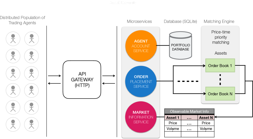
The overall simulation consisted of several programs that intercommunicated to simulate market dynamics (Fig. 1). All market participants (i.e., retail traders, fundamental investors, market makers, etc.) submitted orders in real time over a network via the HTTP protocol to the central system that captured this continuous data feed, facilitated trades and hosted the order books. The central system also hosted a market information server that can be queried on demand at any continuous time $t$ by all agents.

Observation space

Public market information (available to all agents) includes the best bid $p^{bid}_{t}$ and ask $p^{ask}_{t}$ prices, and the current cumulative trading volume $V_{total,t}$. From the bid-ask prices, agents can compute the mid-price defined as $p_{mid,t}=(p^{bid}+p^{ask})/2$. Further, the price history of any asset was also available for all agents to query. In addition, order book information such as the depth of price levels, the number of unique orders at each price level, and the bid or ask side volumes were also available. However, this information was not used by all agents. Private agent-specific details such as available cash, active orders sitting in the order book, and the portfolio composition were restricted to the respective individual agents. Finally, identifying information was also withheld from other market participants, e.g., there is no way to determine who an order was submitted by. Thus, there was no way for an agent to learn a specific individual’s trading pattern and try to predict what they’ll buy/sell next.

Action space

The action space was defined by the discrete actions: (i) The price at which to place a buy order (provided by the use of a limit order); (ii) The price at which to place a sell order (provided by the use of a limit order); (iii) The amount of inventory to immediately trade or hedge (provided by the use of a buy or sell market order); (iv) The amount of pending order to cancel (provided by the use of a cancel order); (v) The option of doing nothing.

Specific agents were endowed with unique privileges; notably, market-making agents were allowed to possess negative inventories and negative cash, which was intentional and realistic due to margin trading and short selling, respectively. All other agent types cannot spend money they don’t have and cannot trade shares they don’t own. Finally, there was no influx of new cash or shares in the simulation, and the total initial amount of cash and shares was conserved.

Figure 1: Schematic of the baseline financial agent-based market simulation architecture. We used a client-server architecture relying on the HTTP protocol for communication where clients (i.e., agents/market participants) communicated with a server (i.e., brokerage/exchange) to fulfill various services (e.g., query account information, submit orders, query market information, etc.). Agent decision-making and order processing were computationally decoupled, which allowed for a realistic setting where trading decisions were made in parallel and orders were processed serially.

2.2 Agents

We used four agent groups to generate trading activity in our simulated market environment: liquidity takers, liquidity providers, market-making agents, and intelligent agents. For simplicity, we avoided using some of the more specific agent types found in the literature, e.g., fundamental, technical, contrarian, etc. [27]. Rather, we considered the liquidity takers and providers as an abstraction of these more specific agents types and used these groups as a stochastic process for modeling supply and demand through market, limit, and cancel orders. The exception to this is the market-making and intelligent agents, which were modeled to represent a specific type of actual market participant, market intermediaries (e.g., market makers, wholesalers, etc.). The pseudo-code for the four agent types in the simulation environment is provided in Appendix A.

2.2.1 Liquidity takers

The liquidity-taking agents were modified from previous work [31], and they were the primary drivers of immediate price movement in the simulation—they removed the best pending orders from the book by submitting market orders exclusively. These agents were activated once the market was open according to a trading frequency parameter. Upon activation time $t$, the activated agent determined how much of their total wealth to devote to risky assets, i.e., they determined their risky wealth $\hat{\mathcal{W}}^{R}_{t}$:

$$\hat{\mathcal{W}}^{R}_{t}=\mathcal{X}_{t}(c_{t}+\sum_{k=1}^{K}h^{k}_{t}\cdot p^{k}_{mid,t}),$$ (1)

where $\mathcal{X}_{t}\sim U\left(0,1\right)$ denotes a random draw from a uniform distribution, $c_{t}$ denotes the agent’s current cash, $h_{t}$ denotes the agent’s current holdings (number of shares) of asset $k$, and $K$ denotes the total number of unique assets. Once the agent’s risky wealth was determined, a Dirichlet distribution with a concentration parameter of 1.0 and $K$ categories was used to randomly determine the new desired portfolio weights $\hat{\omega}_{t+1}^{k}$. Using these new portfolio weights, the agent calculated the number of desired holdings of each asset $k$:

$$\hat{h}_{t+1}^{k}=\left\lfloor\hat{\omega}_{t+1}^{k}\cdot\frac{\hat{\mathcal{W}}^{R}_{t}}{p_{mid,t}^{k}}\right\rfloor$$ (2)

The corresponding order amount $\Delta^{k}_{t}$ was given by:

$$\Delta^{k}_{t}=\hat{h}_{t+1}^{k}-h_{t}^{k}$$ (3)

where $\Delta^{k}_{t}>0$ resulted in a buy market order and $\Delta^{k}_{t}<0$ resulted in a sell market order. Each activated agent repeated this process with their respective observations and properties until market close. These agents are highly scalable and can operate in parallel due to the simplicity of their trading logic and the ability to operate without the need to retain variables in local memory (all variables were instead queried from the brokerage server database at time $t$).

2.2.2 Liquidity providers

The liquidity-providing agents provided price movement resistance to the market—they added pending orders to the book by submitting limit orders exclusively. Identical to liquidity takers, these agents were activated according to a trading frequency parameter between market open and close times. Upon activation time $t$, the activated agent were assigned a limit price $p_{t}^{L_{k}}$ for each asset $k$ by:

$$p_{t}^{L_{k}}=p_{mid,t}^{k}(1+\mathcal{X}),$$ (4)

where $\mathcal{X}\sim\mathcal{N}\left(0,\sigma_{p_{mid,t}^{k}}\right)$ denotes a random draw from a normal distribution with the variance given by a volatility estimate $\sigma_{p_{mid,t}^{k}}$:

$$\sigma_{p_{mid,t}^{k}}=\sqrt{\frac{1}{T}\sum_{t=1}^{T}(r_{t}-\mu)^{2}}$$ (5)

where $r_{t}$ denotes the returns series, $r_{t}=ln(p_{t})-ln(p_{t-1})$, and $\mu$ denotes the mean of the returns series. The agent made trading decisions based on the value of $p_{t}^{L_{k}}$. If $p_{t}^{L_{k}}>p_{mid,t}^{k}$ then the agent would issue a sell limit order for the asset $k$ in their portfolio, and if $p_{t}^{L_{k}}<p_{mid,t}^{k}$ then the agent would use their excess cash and issue a buy limit order to add the asset $k$ to their portfolio. Each activated agent repeated this exercise with their respective observations and properties until market close. Similar to liquidity takers, these agents are highly scalable and can operate in parallel due to the simplicity of their trading logic and the ability to operate without the need to retain variables in local memory.

2.2.3 Market making agents

The market-making agents facilitated trades by placing concurrent orders in the order book and were both providers and takers of liquidity in the simulation. As soon as the market was open, these agents would observe current market conditions and determine the price at which they would place concurrent bid and ask limit orders:

$$p^{bid}_{t}=p_{mid,t}+S_{\text{ref},t}(1+\epsilon_{buy})$$ (6)

$$p^{ask}_{t}=p_{mid,t}-S_{\text{ref},t}(1+\epsilon_{sell})$$ (7)

where $\epsilon_{buy},\epsilon_{sell}\sim U\left(\epsilon_{min},\epsilon_{max}\right)$ denotes random draws from a uniform distribution with the range given by model parameters $\epsilon_{min},\epsilon_{max}$. In general, the price tweak factors $\epsilon$ can be understood as indicators of how passive or aggressive the order is; a trade with $\epsilon>0$ is more passive since it is deeper into the book, and a trade with $\epsilon<0$ is more aggressive since it is quoted at a more competitive price than the pre-existing best quote in the book. After the concurrent limit orders were routed to the central exchange server, the agent would determine how much of their current inventory to hedge. The agent determined the size of the hedge order by multiplying the size of their current inventory $z$ by a random fraction $\mathcal{X}_{t}\sim U\left(0,1\right)$. If $z>0$, they would submit a sell market order; if $z<0$ (i.e., they were in a short position), they would submit a buy market order. The agent would pause to allow the order to be filled, and then they would cancel any unfilled orders and update local variables. The market-making agents repeated this process according to a trading frequency parameter until market close time.

Compared to the liquidity provider and taker agents, the market-making agents are not as scalable due to the speed at which they operate. It is impractical to store their local data (i.e., cash and shares) because they would need to query it so often. Fortunately, the population size of this agent group is low relative to the liquidity provider and taker agents.

2.2.4 Intelligent agents

The intelligent agents were included to mitigate excessively volatile market conditions, as previous work has suggested that strategic behavior is necessary to stabilize trading in order book-driven markets [43]. Intelligent agents were modeled as adaptive market makers and learned to maximize profit while accounting for risk. They used two separate policies to accomplish this: a pricing policy and a hedging policy. The policies were inspired by Ganesh et al. ([44]); each policy utilized estimates of the mean and variance of both the incoming net order flow $\nu_{\epsilon}$ and normalized spread profit-and-loss $s_{\epsilon}$ as a function of $\epsilon^{bid/ask}$. The incoming net order flow $\nu_{\epsilon}$ can be considered the amount of a placed order that is executed. The normalized spread profit-and-loss is defined as $s_{\epsilon}=(\nu S^{bid/ask}_{t})/S_{ref,t}$ for $S^{bid/ask}_{t}=S_{ref,t}(1+\epsilon^{bid/ask})$ and trade size $\nu$.

Empirical estimates

The intelligent agent relied on hand-crafted optimization procedures to execute trading actions for optimal market-making in real-time. These procedures hinged on conditional expectation values $\mathbb{E}(\nu_{\epsilon})$ and $\mathbb{E}(s_{\epsilon})$. For practical reasons, the intelligent agent estimated these values using a linear estimator. Specifically, the estimates were assumed to follow a process given by:

$$y=Ax+e$$

$$\hat{x}=(A^{T}A)^{-1}A^{T}y$$

where $\hat{x}$ denotes the Least-squares estimator and $e$ denotes a Gaussian noise variable with $\mathbb{E}(e)=0$. For the net order flow $\nu_{\epsilon}$, the observed label $y_{\nu}\in\mathbb{R}^{m}$ and the design matrix of given features $A_{\nu}\in\mathbb{R}^{m\times 4}$ was formulated as:

$$y_{\nu}=\begin{bmatrix}\nu_{\epsilon_{t_{0},buy}}\\ \nu_{\epsilon_{t_{0},sell}}\\ \nu_{\epsilon_{t_{1},buy}}\\ \nu_{\epsilon_{t_{1},sell}}\\ \vdots\\ \nu_{\epsilon_{t-1,buy}}\\ \nu_{\epsilon_{t-1,sell}}\end{bmatrix}\quad\quad A_{\nu}=\begin{bmatrix}1.0&p_{mid,t_{0}}&S_{ref,t_{0}}&\epsilon_{t_{0},buy}\\ 1.0&p_{mid,t_{0}}&S_{ref,t_{0}}&\epsilon_{t_{0},sell}\\ 1.0&p_{mid,t_{1}}&S_{ref,t_{1}}&\epsilon_{t_{1},buy}\\ 1.0&p_{mid,t_{1}}&S_{ref,t_{1}}&\epsilon_{t_{1},sell}\\ &&\vdots&\\ 1.0&p_{mid,t-1}&S_{ref,t-1}&\epsilon_{t-1,buy}\\ 1.0&p_{mid,t-1}&S_{ref,t-1}&\epsilon_{t-1,sell}\\ \end{bmatrix}$$

similarly for $s_{\epsilon}$,

$$y_{s}=\begin{bmatrix}s_{\epsilon_{t_{0},buy}}\\ s_{\epsilon_{t_{0},sell}}\\ s_{\epsilon_{t_{1},buy}}\\ s_{\epsilon_{t_{1},sell}}\\ \vdots\\ s_{\epsilon_{t-1,buy}}\\ s_{\epsilon_{t-1,sell}}\end{bmatrix}\quad\quad A_{s}=\begin{bmatrix}1.0&p_{mid,t_{0}}&S_{ref,t_{0}}&\epsilon_{t_{0},buy}&\epsilon_{t_{0},buy}^{2}&\epsilon_{t_{0},buy}^{3}\\ 1.0&p_{mid,t_{0}}&S_{ref,t_{0}}&\epsilon_{t_{0},sell}&\epsilon_{t_{0},sell}^{2}&\epsilon_{t_{0},sell}^{3}\\ 1.0&p_{mid,t_{1}}&S_{ref,t_{1}}&\epsilon_{t_{1},buy}&\epsilon_{t_{1},buy}^{2}&\epsilon_{t_{1},buy}^{3}\\ 1.0&p_{mid,t_{1}}&S_{ref,t_{1}}&\epsilon_{t_{1},sell}&\epsilon_{t_{1},sell}^{2}&\epsilon_{t_{1},sell}^{3}\\ &&&\vdots&&\\ 1.0&p_{mid,t-1}&S_{ref,t-1}&\epsilon_{t-1,buy}&\epsilon_{t-1,buy}^{2}&\epsilon_{t-1,buy}^{3}\\ 1.0&p_{mid,t-1}&S_{ref,t-1}&\epsilon_{t-1,sell}&\epsilon_{t-1,sell}^{2}&\epsilon_{t-1,sell}^{3}\\ \end{bmatrix}$$

where $m$ is the number of observations and $t$ denotes the time that the order was placed. Notably, The estimator for $s_{\epsilon}$ contains two additional features to model the highly curvilinear relationship between $\epsilon$ and the observed normalized spread profit-and-loss. At inference time $t$, the expected value for net order flow for any $\epsilon_{t}$ can be computed using the updated estimator $\hat{x}_{\nu,t}$:

$$\mathbb{E}(\nu_{\epsilon})\approx\left[1.0,p_{mid,t},S_{ref,t},\epsilon_{t}\right]\hat{x}_{\nu,t}$$

and similarly for $\mathbb{E}(s_{\epsilon})$. As the model is deployed over time, rows are continually added to the observation matrix $A$, which makes it challenging and cumbersome to continually compute a new estimate $\hat{x}$. To avoid having to compute an increasingly large matrix inversion, the intelligent agent improved its estimates online via the recursive least-squares (RLS) algorithm.

Similar to the $\mathbb{E}(\nu_{\epsilon})$ and $\mathbb{E}(s_{\epsilon})$ estimates, the optimization procedures also called for variance estimates $var(\nu_{\epsilon})$ and $var(s_{\epsilon})$. These estimates were computed in an online fashion following the procedure given by Knuth [45]. Finally, the intelligent agent also kept an estimate of the market volatility given by $\hat{\sigma}=\sigma\sqrt{\Delta p_{mid}}$.

Pricing policy

The pricing policy follows two steps: at every trade invocation, the intelligent agent chooses price tweaks ($\epsilon_{buy},\epsilon_{sell}$) to meet its market share target $\eta_{ms}$ and reduce its inventory by skewing its quoted prices.

Step 1: Meet target market share. This step ensured that the intelligent agent adapted its policy if it was getting little or no trade flow. Here, the intelligent agent solved for $\epsilon_{*}=\epsilon_{buy}=\epsilon_{sell}$ so that it captured the desired percentage of overall trading volume $\eta_{ms}=$ 25% within tolerance $\delta_{tol}=$ 5% [44]. To accomplish this, the intelligent agent used a time-dependent measurement $V_{market,t}$, which was defined as the observed total trading volume between now and the last trade invocation $V_{market,t}=V_{total,t}-V_{total,t-1}$. The initial step of the policy solved for $\epsilon_{*}$ and was formulated as:

$$\max_{\epsilon}\quad\min_{a} \left|cost_{1}(\epsilon)-cost_{1}(a)\right|$$

s.t. $$\left|cost_{1}(\epsilon)-cost_{1}(a)\right|\leq\delta_{tol}$$

$$cost_{1}(\cdot)=\left|\eta_{ms}-\frac{\mathbb{E(\nu_{\epsilon})}}{V_{market}}\right|$$

where $a$ denotes the estimate for $\epsilon$ that achieves the minimal distance from $\eta_{ms}$. The variable $\epsilon$ converges to $\epsilon_{*}$ and maximizes profit whilst remaining close to $\eta_{ms}$.
Step 2: Skew prices to reduce inventory risk. This step reduced inventory risk by skewing the price of one order side (buy or sell) to attract an order flow that offset the intelligent agent’s current inventory $z$. If the inventory $z$ was negative, it decreased $\epsilon_{buy}$ to attract offsetting buy orders and vice versa. Essentially, this step posed a trade-off between spread profit and inventory risk. The final step of the adaptive pricing policy solved for $\epsilon_{skew}$ and was formulated as:

$$\min_{\epsilon} -S_{ref}\mathbb{E}(s_{\epsilon)}+\gamma\sqrt{S_{ref}^{2}var(s_{\epsilon})+\sigma^{2}\mathbb{E}((z+\nu_{\epsilon})^{2})}$$

where $\gamma=2$ denotes the risk aversion parameter for the model [44]. After step 2 was completed, the $\epsilon$ value for the side that was being skewed was set to $\epsilon_{skew}$, the other was set to $\epsilon_{*}$, and the limit order was sent over the network. Next, the intelligent agent conducted the hedging policy.

Hedging policy

Similar to step 2 of the pricing policy, the hedging policy aimed to reduce risk by leveraging opposing trades—only here, instead of setting prices in the hope of attracting an offsetting trade, the intelligent agent directly executed the offsetting trade themselves. The trade-off was between the cost of hedging (by crossing the spread) and inventory risk. The fraction of current inventory to hedge $x$ was formulated as:

$$\min_{x} \left|xz\right|S_{ref}+\gamma\sqrt{\sigma^{2}\mathbb{E}((z(1-x)+\nu_{\epsilon})^{2})}$$

s.t. $$z(1-x)=Z$$

$$0\leq x\leq 1$$

$$-3000\leq Z\leq 3000$$

where the new inventory $Z$ respects the bounds estimated by empirical high-frequency trading studies [46]. The intelligent agent requires more computational resources to operate than the other agent types and relies on a growing design matrix $A$, which inhibits the scalability of the model. In our simulation trials, we only operated a single intelligent agent and ran it on a different machine. Further, we limited this agent to operating on a single asset and excluded it from our multi-asset simulation trials. We leave optimization efforts to the intelligent agent (e.g., exponential forgetting factors, sliding window techniques for growing data matrix, etc. [47, 48]) and the design of more intelligent agent types (e.g., deep learning agents) to future work.

3 Results and Discussion

3.1 Calibration and stable generation of synthetic financial time series data

(a)

(b)

(c)

(d)

Figure 2: The intelligent agent type effectively stabilized the market environment. (a) Two market-making agents induced relatively volatile bid (blue) and ask (orange) prices, characterized by large upward and downward price movements. (b) One market making agent and one intelligent agent induced stable bid (blue) and ask (orange) prices. (c) Two market-making agents induced large bid-ask spreads (difference between the bid and ask prices) and an overall illiquid market environment characterized by frequent jumps in the cost of trading (crossing the spread). (d) One market-making agent and one intelligent agent induced a stable bid-ask spread and resilient market liquidity.

We considered three simulation cases: small-scale univariate time series generation, medium-scale multivariate time series generation, and large-scale multivariate time series generation (Table 1). The liquidity taker and provider agents were defined by four parameters: the number of agents, the initial cash range, the initial shares range, and the agent trading frequency. Each agent’s initial cash and share allotment was determined through a draw from a uniform distribution bounded by the range parameters. The market-making agents were defined by four parameters: the number of agents, the price deviation bounds (constant values $\epsilon_{min}=-0.5$ and $\epsilon_{max}=1.0$ [44]), the unit trade size (constant value of 100, which is a typical lot size [6]), and the trading frequency. The intelligent agents were defined by six parameters: the market share target ($\eta_{ms}=$ 25%), risk aversion ($\gamma=2$ ), tolerance ($\delta_{tol}=$ 5%), inventory limit (3000), unit trade size (100), and trading frequency. The market-making and intelligent agents were instantiated with zero cash and zero shares (but were allowed to borrow cash and shares).

Table 1: Model parameters for each simulation case.

Parameter	Small univariate	Medium multivariate	Large multivariate
Liquidity Takers (LT)	70	650	8000
Liquidity Providers (LP)	70	5850	100000
Market Makers (MM)	1	200	500
Intelligent Agents (IA)	1	0	0
Initial cash range	$5,000 - $15,000	$25,000 - $75,000	$150,000 - $450,000
Initial shares range (per asset)	50 - 150	50 - 150	50 - 150
Trading frequencies (seconds)	LT=5, LP=10, MM=2, IA=2	LT=720, LP=720, MM=2	LT=7200, LP=7200, MM=2
Number of unique assets	1	5	30

We based the simulation’s initialization and calibration procedures on previous empirical market studies [49, 46]. We adjusted these parameters according to our case study’s objectives and available computational resources. We found that poorly calibrated parameters led to adverse effects, such as unrealistic liquidity and price movement, which were more noticeable when simulating larger agent populations. Specifically, the simulation performance was sensitive to liquidity takers and providers’ initial cash and shares allotment range. If the total initial cash and market value of all assets were roughly equal, the resulting aggregate time series was unbiased. However, if the total initial value of shares was higher than the total initial value of cash, simulation trials were biased toward share prices falling and vice versa. This was a notable feature of our ABM, which suggests that the conservation of total agent cash and shares constraints led to meaningful supply and demand phenomena. To ensure fairness, we used a distribution with a high probability of equal values of total cash and shares in each simulation trial. We set the initial mid-price and random initial order book arrangements for each case study. The parameters for each case study are listed in Table 1.

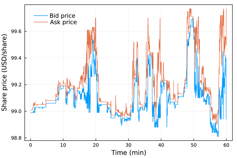
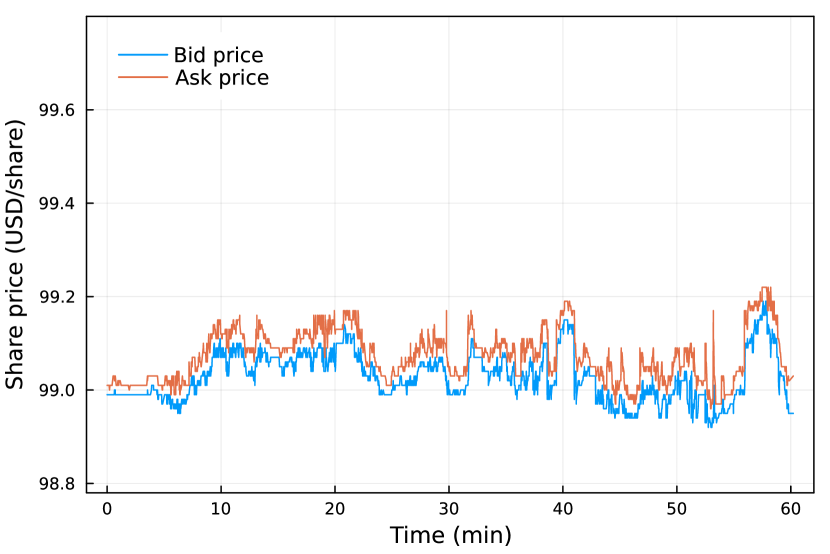
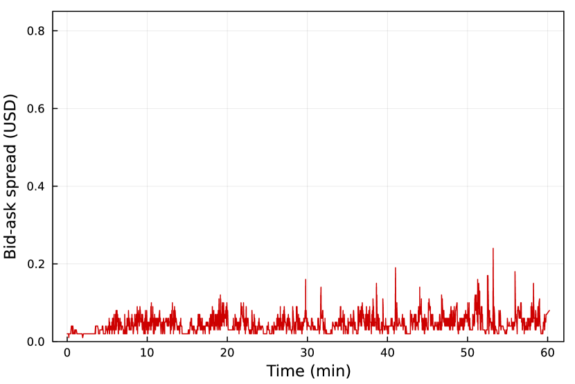
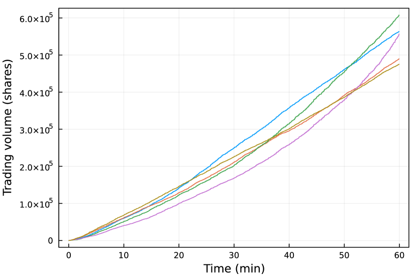
The addition of the intelligent agent effectively stabilized the small-scale univariate simulation environment (Fig. 2). The intelligent agent consistently outperformed other market marking agents and demonstrated a profit in each simulation run. Interestingly, the intelligent agent accomplished this despite the high degree of noise in the environment and the relative simplicity of its linear model. However, upon inspection, we found that the intelligent agent’s model produced a poor estimation fit, suggesting that more sophisticated intelligent agents could dominate in this market environment and that more work is needed to produce more realistic odds of profitability in our simulated market.

3.2 Validation of synthetic financial time series data

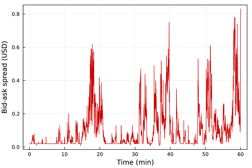
The baseline financial ABM captured several empirical properties of financial time series (Fig. 3). To gauge the efficacy of our baseline ABM and validate our approach, we tested our synthetic time series for the presence of several common univariate stylized facts. We evaluated ten simulation trials of the small-scale univariate case, each sample consisting of an hour’s worth of simulated data, and our findings were consistent across all trials.

(a)

(b)

(c)

(d)

(e)

(f)

Figure 3: Stylized facts for the time series generated by the baseline financial ABM. (a) Heavy-tailed returns distribution is demonstrated by the high and narrow peak at zero return and the slow decay at the margins of the distribution. (b) Linear unpredictability is demonstrated by the lack of autocorrelation of price returns except at very short time horizons. (c) Volatility clustering is demonstrated by significant positive autocorrelation of price volatility. (d) Nonlinear dependence is demonstrated by significant positive autocorrelation of nonlinear functions of returns (i.e., $|r|$, $r^{2}$, $|r^{2}|$, $cos(r)$, and $log(1+r^{2})$). (e) Gain/loss asymmetry demonstrated by the distribution of first passage times $\tau_{\rho}$ when an asset crosses a fixed return level $\rho$ (where $\rho$ = $\pm$ 5$\times$ standard deviation of the price series). (f) Aggregational gaussianity is demonstrated by the returns distribution’s increasing resemblance to a normal distribution as the time scale over which returns are calculated is increased (i.e., we compare returns calculated from (i) every price tick to (ii) every other price tick and (iii) every fifth price tick). For panels (b)-(d), the autocorrelation series vs. a 95% confidence interval for a random walk is shown.

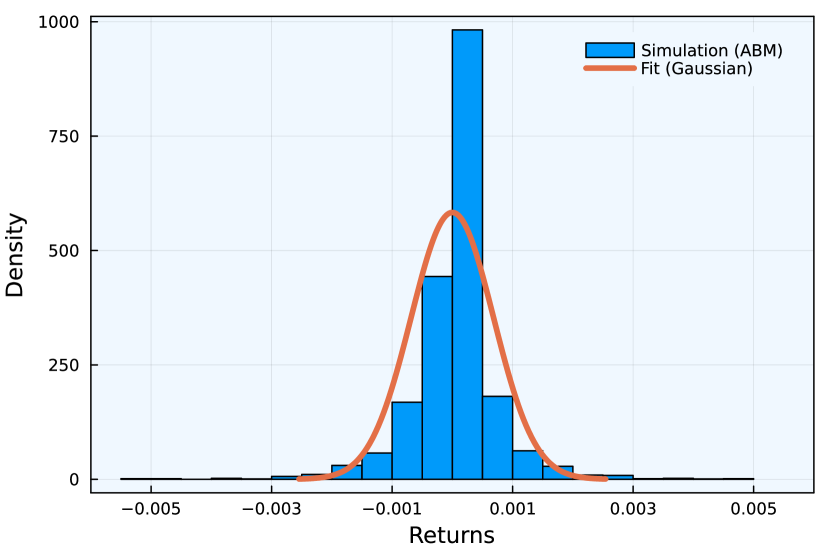
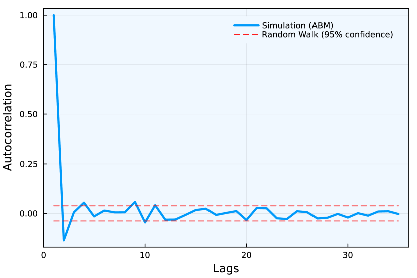
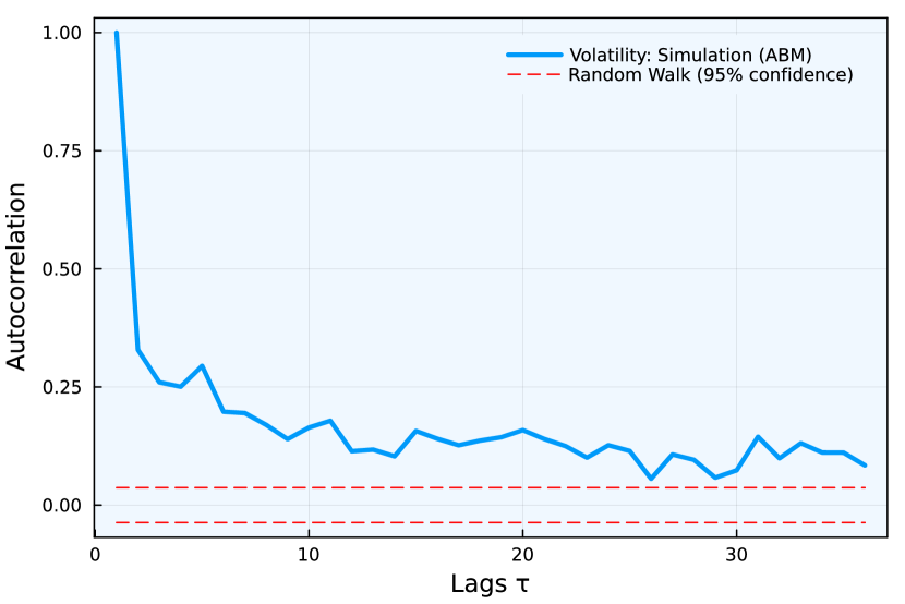
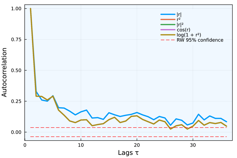
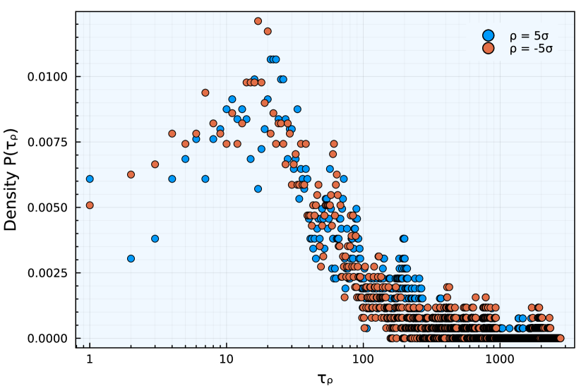
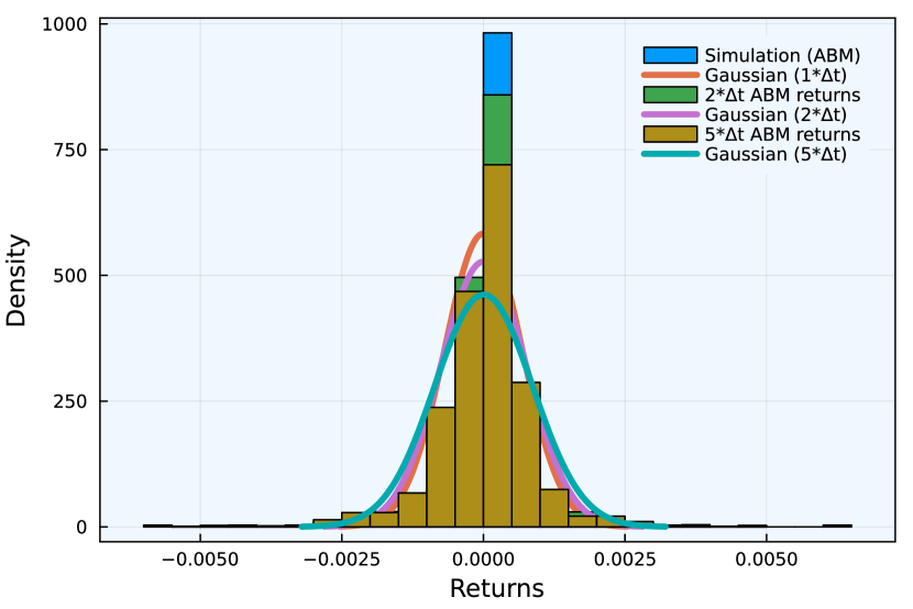
These results indicated that the structure of markets (i.e., double auction mechanism, uncertain order fulfillment, etc.), rather than fully rational agent behavior, was enough to account for several statistical regularities of financial markets. These findings are consistent with other zero-intelligence studies in the literature [30, 7]. There are, however, several statistical properties that we were unable to account for using this baseline ABM. Stylized facts that relate to volume (e.g., long memory of volume, volume-volatility correlation) were not captured by our model. This is unsurprising, considering that our baseline agents were not conditioned on volume and were not reactive (i.e., they did not trade/activate based on a conditional signal but rather according to a constant trading frequency). Similarly, the "leverage effect" stylized fact was not captured, and we found this reasonable considering that our zero-intelligence agents possessed no notion of historical performance or personal utility. Further, our baseline agent behaviors were unequipped to replicate stylized facts such as intraday volume patterns (open and close times are not factored into agent behavior) and cross-asset correlations (company sectors are not included in the observation space). The ABM will require extensions to accommodate these and other statistical properties that were unable to be replicated in our baseline implementation. We leave this to future work.

The addition of the intelligent agent had minor impacts on the stylized facts exhibited by the baseline ABM. The only difference was that without the intelligent agent, the generated time series were more volatile, and the presence of stylized facts related to volatility was more pronounced and deviated from what was observed empirically. We suspect that the reason no additional stylized facts were observed with the inclusion of the intelligent agent was likely because its decision-making was conditioned on the same price-centric feature variables as all other agents rather than new ones such as volume and historical trends (e.g., simple moving average and other rolling statistics).

3.3 Large-scale generation of synthetic financial time series data

Our large-scale simulation trials consisted of multiple unique assets and several thousand agents operating across multiple machines (Fig.  4). For the large-scale trials, we split the central server and agents across three machines that were each equipped with an Intel Core i7-6700 CPU and Ubuntu 22.04. Our machine allotment for each simulation component was based on minimizing computational bottlenecks: the central system (server hosting order books and observable variables) was allotted its own machine, the market-making agents (high-frequency market intermediaries) operated on a single machine, and the liquidity providers and takers (low-frequency traders) were both operated on the single remaining machine.

(a)

(b)

(c)

(d)

Figure 4: Price and volume series for the multivariate simulation trials. (a) Synthetic price series for each of the five assets of the medium-scale multivariate simulation case. (b) Synthetic market volume series or cumulative shares traded, for each of the five assets of the medium-scale multivariate simulation case. (c) Synthetic price series for each of the 30 assets of the large-scale multivariate simulation case. (d) Synthetic market volume series or cumulative shares traded for each of the 30 assets of the large-scale multivariate simulation case.

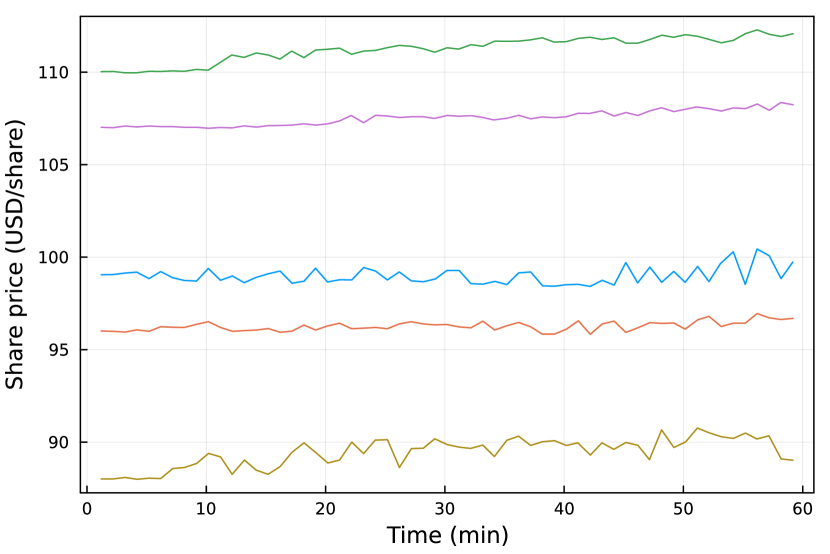
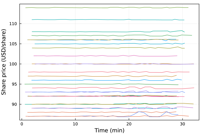
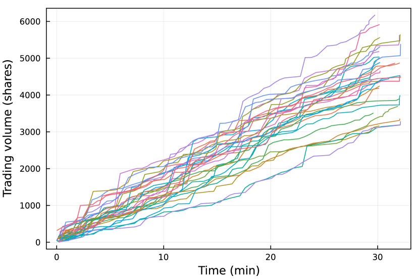
The initial share prices of the assets were drawn from a uniform distribution bounded by $85.00 and $115.00. Our results demonstrated how the baseline ABM could support multiple simultaneous assets by only using basic agent types and modest computational resources. With greater resources, it would be straightforward to scale the simulation even further–opening up possibilities to explore multivariate stylized facts and investigate more complicated agent behaviors. For instance, a large-scale ABM would allow researchers to investigate portfolio management agent behaviors and trading differences between small-tick and large-tick stocks.

Although the baseline ABM was capable of supporting large agent populations and many available assets, the scale of trading activity (i.e., executed orders or transactions) was hindered by the use of a single central system for both order processing and retrieving observable information. For instance, after 30 minutes, the medium-scale simulation trial produced approximately 45,000 trades across all assets, and the large-scale simulation trial produced only 2,000. We suspect that this is due to the large message load induced on the single gateway to the central server and the look-up times associated with the large SQLite database. To simulate realistic large-scale trading activity, components of the baseline ABM will have to be further optimized and partitioned (e.g., the communication should be optimized, and the brokerage functionality of the central system should be isolated from the exchange/order books segment). We leave this to future work.

4 Summary and Conclusion

This study introduced a baseline financial ABM that scaled to several thousand agents, supports multiple simultaneous assets, captured intuitive supply and demand dynamics, and demonstrated several well-known statistical properties of financial markets. Further, our ABM does all of this without the inclusion of traditional agent behaviors (e.g., fundamental, technical, etc.) or the need for historical market data. That being said, the ABM can be readily extended to support additional agent types and will need to do so in order to improve on realism and capture additional stylized facts. In particular, our results emphasize the need to include conditional activation times for agents and agent behaviors that are conditioned on variables such as historical price performance metrics, market sectors, and time of day. We cannot conclude that intelligent agent behaviors are needed for the reproduction of stylized facts, but our results do suggest that intelligent agent behavior may be needed for resilient market liquidity. Moreover, we suspect that the inclusion of several intelligent agent types and competition among them will be necessary to produce more realistic probability odds in the simulation. Additional ways to improve simulation fidelity of the baseline ABM, especially at large scale, include the reorganization of simulation components and the adoption of low-latency and high-throughput communication frameworks.

Data availability statement

This work was produced using the Brokerage.jl and TradingAgents.jl Julia packages. Model codes are available at: https://github.com/aaron-wheeler/Brokerage.jl.git and https://github.com/aaron-wheeler/TradingAgents.jl.git.

Appendix A. Trading agent algorithms

Here, we provide pseudo-code for the agents in the simulation environment. Agent behaviors followed one of four types: liquidity takers (Algorithm 1), liquidity providers (Algorithm 2), market makers (Algorithm 3), and intelligent market makers (Algorithm 4).

Data: Market state ($t,p_{mid}$),

     agent parameters ($c_{min},c_{max},h_{min},h_{max},t_{freq}$),

     and simulation parameters ($N,K,T_{close}$)

Result: Consistent market order (MO) flow for duration of simulation

/* Initialize agents */

for agent $n\in N$ do

       $c_{n,t_{0}}\leftarrow U(c_{min},c_{max})$;

       foreach asset $k\in K$ do $h_{n,t_{0}}^{k}\leftarrow U(h_{min},h_{max})$;

      

end for

/* Execute trades */

while $t<T_{close}$ do

       for agent $n\in N$ do

             Sample $u_{n,t}$ $\sim$ U(0, 1)

             if $u_{n,t}$ < $\frac{1}{t_{freq}}$ then

                   Sample risk fraction $\mathcal{X}_{n,t}$ $\sim$ U(0, 1)

                   $\hat{\mathcal{W}}^{R}_{n,t}\leftarrow\mathcal{X}_{n,t}(c_{n,t}+\sum_{k=1}^{K}h^{k}_{n,t}\cdot p^{k}_{mid,t})$;

                   Sample portfolio weights $\hat{\omega}_{n,t+1}^{k}$ $\sim$ D($K$, 1.0)

                   for asset $k\in K$ do

                         $\hat{h}_{n,t+1}^{k}\leftarrow\left\lfloor\hat{\omega}_{n,t+1}^{k}\cdot\frac{\hat{\mathcal{W}}^{R}_{n,t}}{p_{mid,t}^{k}}\right\rfloor$ ;

                         $\Delta^{k}_{n,t}\leftarrow\hat{h}_{n,t+1}^{k}-h_{n,t}^{k}$ ;

                         if $\Delta^{k}_{n,t}<0$ then

                               Submit buy side MO with volume $\Delta^{k}_{n,t}$;

                              

                        else

                               Submit sell side MO with volume $\Delta^{k}_{n,t}$;

                              

                         end if

                        

                   end for

                  

             end if

            

       end for

      

end while

Algorithm 1 Liquidity taker agent algorithm

Data: Market state ($t,p_{bid},p_{ask},p_{h}:\forall h=0,1,\ldots,t$),

     agent parameters ($c_{min},c_{max},h_{min},h_{max},t_{freq}$),

     and simulation parameters ($N,K,T_{close}$)

Result: Consistent limit order (LO) flow for duration of simulation

/* Initialize agents */

for agent $n\in N$ do

       $c_{n,t_{0}}\leftarrow U(c_{min},c_{max})$;

       foreach asset $k\in K$ do $h_{n,t_{0}}^{k}\leftarrow U(h_{min},h_{max})$;

      

end for

/* Execute trades */

while $t<T_{close}$ do

       foreach asset $k\in K$ do $p_{mid,t}^{k}\leftarrow\frac{p_{bid,t}^{k}+p_{ask,t}^{k}}{2}$;

       for agent $n\in N$ do

             Sample $u_{n,t}$ $\sim$ U$(0,1)$

             if $u_{n,t}$ < $\frac{1}{t_{freq}}$ then

                   for asset $k\in K$ do

                         $r_{t}^{k}\leftarrow\sum_{t=1}^{T}ln(p_{t}^{k})-ln(p_{t-1}^{k})$;

                         $\mu\leftarrow\frac{1}{T}\sum_{t=1}^{T}(r_{t}^{k})$;

                         $\sigma_{p_{mid,t}^{k}}\leftarrow\sqrt{\frac{1}{T}\sum_{t=1}^{T}(r_{t}-\mu)^{2}}$;

                         Sample $\mathcal{X}_{n,t}\sim\mathcal{N}\left(0,\sigma_{p_{mid,t}^{k}}\right)$;

                         $p_{n,t}^{L_{k}}\leftarrow p_{mid,t}^{k}(1+\mathcal{X}_{n,t})$;

                        

                   end for

                  for asset $k\in K$ do

                         if $h^{k}_{n,t}>0$ and $p_{mid}<p_{n,t}^{L_{k}}$ then

                               $\Delta^{k}_{n,t}\leftarrow U(0,1)\ast h^{k}_{n,t}$;

                               Submit sell side LO with volume $\Delta^{k}_{n,t}$ and limit price $max\left\{p_{ask,t},p_{n,t}^{L_{k}}\right\}$;

                              

                         end if

                        

                   end for

                  for eligible assets $k_{e}\in K_{e}$ where $K_{e}=count(c_{n,t}>p_{mid,t}^{k})$ do

                         Sample cash allocation for eligible assets $\hat{c}_{n,t}^{k}$ $\sim$ D$(K_{e},1.0)$;

                         for eligible assets $k_{e}\in K_{e}$ do

                               $\Delta^{k}_{n,t}\leftarrow\left\lfloor\hat{c}_{n,t}^{k}\cdot\frac{c_{n,t}}{\text{min}\left\{p_{bid,t},p_{n,t}^{L_{k}}\right\}}\right\rfloor$ ;

                               Submit buy side LO with volume $\Delta^{k}_{n,t}$ and limit price $min\left\{p_{bid,t},p_{n,t}^{L_{k}}\right\}$;

                              

                         end for

                        

                   end for

                  

             end if

            

       end for

      

end while

Algorithm 2 Liquidity provider agent algorithm

Data: Market state ($t,p_{mid},S_{ref}$),

     agent parameters ($\epsilon_{min},\epsilon_{max},O_{size},t_{freq}$),

     and simulation parameters ($N,K,T_{close}$)

Result: Consistent liquidity across assets for duration of simulation

/* Initialize agents */

for agent $n\in N$ do

       $c_{n,t_{0}}\leftarrow 0$;

       foreach asset $k\in K$ do $z_{n,t_{0}}^{k}\leftarrow 0$;

      

end for

/* Execute trades */

while $t<T_{close}$ do

       for agent $n\in N$ do

             Sample $u_{n,t}$ $\sim$ U$(0,1)$

             if $u_{n,t}$ < $\frac{1}{t_{freq}}$ then

                   for asset $k\in K$ do

                         $\epsilon_{buy}^{k}\leftarrow U(\epsilon_{min},\epsilon_{max})$;

                         $\epsilon_{sell}^{k}\leftarrow U(\epsilon_{min},\epsilon_{max})$;

                         $p^{bid_{k}}_{t}\leftarrow p_{mid,t}^{k}+S_{ref,t}^{k}(1+\epsilon_{buy}^{k})$;

                         $p^{ask_{k}}_{t}\leftarrow p_{mid,t}^{k}-S_{ref,t}^{k}(1+\epsilon_{sell}^{k})$;

                         Submit buy and sell side LOs with volume $O_{size}$ and limit price $p^{bid_{k}}_{t}$ and $p^{ask_{k}}_{t}$, respectively;

                         begin

                               Sample hedge fraction $\mathcal{X}_{n,t}$ $\sim$ $U(0,1)$;

                               $O_{hedge}\leftarrow\mathcal{X}_{n,t}\ast z_{n,t}^{k}$;

                               if $z_{n,t}^{k}>0$ then

                                     Submit sell side MO with volume $O_{hedge}$;

                                    

                              else

                                     Submit buy side MO with volume $O_{hedge}$;

                                    

                               end if

                              

                         end

                        

                        if Order is not filled then

                               Cancel all unfilled buy and sell LOs;

                              

                         end if

                        Update cash $c_{n,t}$ and inventory $z_{n,t}^{k}$;

                        

                   end for

                  

             end if

            

       end for

      

end while

Algorithm 3 Market making agent algorithm

Data: Market state ($t,p_{mid},S_{ref},V_{total}$),

     agent parameters ($\eta_{ms},\gamma,\delta_{tol},Z,O_{size},t_{freq}$),

     and simulation parameters ($T_{close}$)

Result: Strategic trading activity for single asset for duration of simulation

/* Initialize agent */

$c_{t_{0}}\leftarrow 0$;

$z_{t_{0}}^{k}\leftarrow 0$;

/* Execute trades for single asset */

while $t<T_{close}$ do

       $\hat{\sigma}\leftarrow\sigma\sqrt{p_{mid,t}-p_{mid,t-1}}$;

       $V_{M}\leftarrow V_{total,t}-V_{total,t-1}$;

       $\epsilon_{\ast}\leftarrow$ PricingPolicyTarget($\eta_{ms},\delta_{tol},V_{M},\mathbb{E}(\nu_{\epsilon})$);

       $\epsilon_{skew}\leftarrow$ PricingPolicySkew($S_{ref},\mathbb{E}(s_{\epsilon}),\gamma,var(s_{\epsilon}),\sigma,var(\nu_{\epsilon})$);

       if $z>0$ then

             $p^{bid}_{t}\leftarrow p_{mid,t}+S_{ref,t}(1+\epsilon_{\ast})$;

             $p^{ask}_{t}\leftarrow p_{mid,t}-S_{ref,t}(1+\epsilon_{skew})$;

            

      else

             $p^{bid}_{t}\leftarrow p_{mid,t}+S_{ref,t}(1+\epsilon_{skew})$;

             $p^{ask}_{t}\leftarrow p_{mid,t}-S_{ref,t}(1+\epsilon_{\ast})$;

            

       end if

      Submit buy and sell side LOs with volume $O_{size}$ and limit price $p^{bid}_{t}$ and $p^{ask}_{t}$, respectively;

       Solve for hedge fraction $\mathcal{X}_{t}\leftarrow$ HedgePolicy($z_{t},S_{ref},\gamma,\sigma,var(\nu_{\epsilon}),Z$);

       $O_{hedge}\leftarrow\mathcal{X}_{t}\ast z_{t}^{k}$;

       if $z_{t}>0$ then

             Submit sell side MO with volume $O_{hedge}$;

            

      else

             Submit buy side MO with volume $O_{hedge}$;

            

       end if

      while $V_{total,t}==V_{total,t-1}$ do

             Wait($t_{freq}$);

            

       end while

      if Order is not filled then

             Cancel all unfilled buy and sell LOs;

            

       end if

      Update cash $c_{t}$ and inventory $z_{t}$;

       Update observation matrices $A_{\nu}$ and $A_{s}$;

       Update measurement vectors $\nu_{t}$ and $s_{t}$;

       $\hat{x}_{\nu,t},P_{\nu,t},K_{\nu,t}\leftarrow$ RLS($\hat{x}_{\nu,t-1},P_{\nu,t-1},K_{\nu,t-1},A_{\nu},\nu_{t}$);

       $\hat{x}_{s,t},P_{s,t},K_{s,t}\leftarrow$ RLS($\hat{x}_{s,t-1},P_{s,t-1},K_{s,t-1},A_{s},s_{t}$);

      

end while

Algorithm 4 Intelligent agent algorithm

References

- [1] Maureen O’Hara. Market Microstructure Theory. Blackwell, London, England, November 1997.
- [2] James Paulin, Anisoara Calinescu, and Michael Wooldridge. Agent-based modeling for complex financial systems. IEEE Intelligent Systems, 33(2):74–82, March 2018.
- [3] Martin D. Gould, Mason A. Porter, Stacy Williams, Mark McDonald, Daniel J. Fenn, and Sam D. Howison. Limit order books. Quantitative Finance, 13(11):1709–1742, November 2013.
- [4] Jean-Philippe Bouchaud, J. Doyne Farmer, and Fabrizio Lillo. How markets slowly digest changes in supply and demand, 2008.
- [5] R. Cont. Empirical properties of asset returns: stylized facts and statistical issues. Quantitative Finance, 1(2):223–236, February 2001.
- [6] Anirban Chakraborti, Ioane Muni Toke, Marco Patriarca, and Frédéric Abergel. Econophysics review: I. empirical facts. Quantitative Finance, 11(7):991–1012, June 2011.
- [7] Svitlana Vyetrenko, David Byrd, Nick Petosa, Mahmoud Mahfouz, Danial Dervovic, Manuela Veloso, and Tucker Balch. Get real. In Proceedings of the First ACM International Conference on AI in Finance. ACM, October 2020.
- [8] Benoit Mandelbrot. The variation of certain speculative prices. The Journal of Business, 36(4):394, January 1963.
- [9] Benoit Mandelbrot. Analysis of long-run dependence in economics-r/s technique. In Econometrica, volume 39, pages 68–+. WILEY-BLACKWELL 111 RIVER ST, HOBOKEN 07030-5774, NJ USA, 1971.
- [10] Parameswaran Gopikrishnan, Vasiliki Plerou, Luís A. Nunes Amaral, Martin Meyer, and H. Eugene Stanley. Scaling of the distribution of fluctuations of financial market indices. Physical Review E, 60(5):5305–5316, November 1999.
- [11] Robert F. Engle. Autoregressive conditional heteroscedasticity with estimates of the variance of united kingdom inflation. Econometrica, 50(4):987, July 1982.
- [12] Rama Cont. Long range dependence in financial markets. In Fractals in Engineering, pages 159–179. Springer-Verlag.
- [13] Johannes Vitalis Siven and Jeffrey Todd Lins. Gain/loss asymmetry in time series of individual stock prices and its relationship to the leverage effect, 2009.
- [14] Jean-Philippe Bouchaud, Marc Mézard, and Marc Potters. Statistical properties of stock order books: empirical results and models. Quantitative Finance, 2(4):251–256, August 2002.
- [15] James H. Stock and Mark W. Watson. Testing for common trends. Journal of the American Statistical Association, 83(404):1097–1107, December 1988.
- [16] Vasiliki Plerou, Parameswaran Gopikrishnan, Bernd Rosenow, Luís A. Nunes Amaral, Thomas Guhr, and H. Eugene Stanley. Random matrix approach to cross correlations in financial data. Physical Review E, 65(6), June 2002.
- [17] Didier Sornette. Physics and financial economics (1776–2014): puzzles, ising and agent-based models. Reports on Progress in Physics, 77(6):062001, May 2014.
- [18] Zhi-Qiang Jiang, Wen-Jie Xie, Wei-Xing Zhou, and Didier Sornette. Multifractal analysis of financial markets: a review. Reports on Progress in Physics, 82(12):125901, November 2019.
- [19] John C. Cox, Stephen A. Ross, and Mark Rubinstein. Option pricing: A simplified approach. Journal of Financial Economics, 7(3):229–263, September 1979.
- [20] Robert Engle. GARCH 101: The use of ARCH/GARCH models in applied econometrics. Journal of Economic Perspectives, 15(4):157–168, November 2001.
- [21] A. C. Harvey. ARIMA models. In Time Series and Statistics, pages 22–24. Palgrave Macmillan UK, 1990.
- [22] James H Stock and Mark W Watson. Vector autoregressions. Journal of Economic Perspectives, 15(4):101–115, November 2001.
- [23] Fischer Black and Myron Scholes. The pricing of options and corporate liabilities. Journal of Political Economy, 81(3):637–654, May 1973.
- [24] R Axtell and J Farmer. Agent based modeling in economics and finance: past, present, and future. Journal of Economic Literature, 2022.
- [25] W. Brian Arthur. Foundations of complexity economics. Nature Reviews Physics, 3(2):136–145, January 2021.
- [26] Jean-Philippe Bouchaud. Radical complexity. Entropy, 23(12):1676, December 2021.
- [27] Shu-Heng Chen, Chia-Ling Chang, and Ye-Rong Du. Agent-based economic models and econometrics. The Knowledge Engineering Review, 27(2):187–219, April 2012.
- [28] J. von Neumann and O. Morgenstern. Theory of games and economic behavior. Princeton University Press, 1947.
- [29] Blake LeBaron, W.Brian Arthur, and Richard Palmer. Time series properties of an artificial stock market. Journal of Economic Dynamics and Control, 23(9-10):1487–1516, September 1999.
- [30] J. Doyne Farmer, Paolo Patelli, and Ilija I. Zovko. The predictive power of zero intelligence in financial markets, 2003.
- [31] L. Ponta, M. Raberto, and S. Cincotti. A multi-assets artificial stock market with zero-intelligence traders. EPL (Europhysics Letters), 93(2):28002, January 2011.
- [32] Marco Raberto, Silvano Cincotti, Sergio M. Focardi, and Michele Marchesi. Agent-based simulation of a financial market. Physica A: Statistical Mechanics and its Applications, 299(1-2):319–327, October 2001.
- [33] Chia-Hsuan Kuo, Chiao-Ting Chen, Sin-Jing Lin, and Szu-Hao Huang. Improving generalization in reinforcement learning–based trading by using a generative adversarial market model. IEEE Access, 9:50738–50754, 2021.
- [34] Leo Ardon, Nelson Vadori, Thomas Spooner, Mengda Xu, Jared Vann, and Sumitra Ganesh. Towards a fully rl-based market simulator. In Proceedings of the Second ACM International Conference on AI in Finance. ACM, November 2021.
- [35] David Byrd, Maria Hybinette, and Tucker Hybinette Balch. Abides: Towards high-fidelity market simulation for ai research, 2019.
- [36] Johann Lussange, Stefano Vrizzi, Sacha Bourgeois-Gironde, Stefano Palminteri, and Boris Gutkin. Stock price formation: Precepts from a multi-agent reinforcement learning model. Computational Economics, April 2022.
- [37] Olivier Brandouy, Philippe Mathieu, and Iryna Veryzhenko. On the design of agent-based artificial stock markets. In Communications in Computer and Information Science, pages 350–364. Springer Berlin Heidelberg, 2013.
- [38] Ivan Jericevich, Patrick Chang, and Tim Gebbie. Simulation and estimation of an agent-based market-model with a matching engine, 2021.
- [39] Francesco Lamperti, Andrea Roventini, and Amir Sani. Agent-based model calibration using machine learning surrogates, 2017.
- [40] Aldo Glielmo, Marco Favorito, Debmallya Chanda, and Domenico Delli Gatti. Combining search strategies to improve performance in the calibration of economic abms, 2023.
- [41] Johannes Dahlke, Kristina Bogner, Matthias Mueller, Thomas Berger, Andreas Pyka, and Bernd Ebersberger. Is the juice worth the squeeze? machine learning (ml) in and for agent-based modelling (abm), 2020.
- [42] Jeff Bezanson, Alan Edelman, Stefan Karpinski, and Viral B Shah. Julia: A fresh approach to numerical computing. SIAM Review, 59(1):65–98, 2017.
- [43] Anirban Chakraborti, Ioane Muni Toke, Marco Patriarca, and Frederic Abergel. Econophysics: Empirical facts and agent-based models. 2009.
- [44] Sumitra Ganesh, Nelson Vadori, Mengda Xu, Hua Zheng, Prashant Reddy, and Manuela Veloso. Reinforcement learning for market making in a multi-agent dealer market, 2019.
- [45] Donald E. Knuth. The Art of Computer Programming, The: Seminumerical Algorithms, volume 2. Addison-Wesley Professional, 3 edition, 1997.
- [46] ANDREI KIRILENKO, ALBERT S. KYLE, MEHRDAD SAMADI, and TUGKAN TUZUN. The flash crash: High-frequency trading in an electronic market. The Journal of Finance, 72(3):967–998, April 2017.
- [47] A. Vahidi, A. Stefanopoulou, and H. Peng. Recursive least squares with forgetting for online estimation of vehicle mass and road grade: theory and experiments. Vehicle System Dynamics, 43(1):31–55, January 2005.
- [48] Qinghua Zhang. Some implementation aspects of sliding window least squares algorithms. IFAC Proceedings Volumes, 33(15):763–768, June 2000.
- [49] Mark Paddrik, Roy Hayes, Andrew Todd, Steve Yang, Peter Beling, and William Scherer. An agent based model of the e-mini sp500 applied to flash crash analysis. In 2012 IEEE Conference on Computational Intelligence for Financial Engineering and Economics (CIFEr). IEEE, March 2012.