Weak Coupling Regime in Dilatonic $f\left(R,T\right)$ Cosmology

Abstract

We consider $f(R,T)$ modified theories of gravity in the context of string theory inspired dilaton gravity. We addressed two specific models to check how they can display the inflationary early Universe and late time cosmology by addressing the choice of parameters in accord with observational data in modern cosmology. We employ numerical methods to obtain several important observable quantities.

I Introduction

Modern observations in cosmology, performed from Type Ia Supernova (SNIa)riess-pearlmutter , Large Scale Structure (LSS)lss , Wilkinson Microwave Anisotropy Probe (WMAP)wmap data, Cosmic Microwave Background (CMB)cbm and Baryonic Acoustic Oscillations (BAO)bao indicate that the expansion of the Universe has entered an accelerated phase. Furthermore, the same observational data show that $95\%$ of the matter and energy content of the Universe (when described in terms of a fluid effectively entering Einstein’s equations) is in the form of unknown species called Dark Matter (DM) and Dark Energy (DE). General Relativity has always been consistent with observational data and one of the most recent examples is the detection of gravitational waves through LIGO ligo . General Relativity analyzes the acceleration of the universe based on dark energy, according to observations of type Ia supernovae, which counterbalances gravitational attraction. The Dark Energy pad.1 ; frie ; martin ; cald ; silve ; bamba ; li ; sami component ($\rho_{x}$) is characterized by a negative effective pressure, $p_{x}<-\rho_{x}/3$. The simplest candidate for such a dark energy is a positive cosmological constant $\Lambda$, but such an identification raises some difficult questions, such as why $\Lambda$ is so small (in particle physics) peeb ; pad.2 ; sahni . This is called the fine-tuning problem for $\Lambda$. Another important problem is why $\Lambda=\rho_{x0}$ in present epoch (where $\rho_{x0}$ is the present value of the dark energy density of the Universe, in Planck units). This problem is known as cosmic coincidence velt . A promising way to solve the above problems is to introduce a single scalar field, dubbed the quintessence shinji , whose potential goes asymptotically to zero (solving the cosmological constant problem). The potential associated with this scalar field tends to zero as the field goes to infinity after an infinite (very long) time. On the other hand, we can try to reconcile the observational data with the acceleration of the Universe through modifications of the theory of gravity. One way to do this is to start with a modification of the Einstein-Hilbert action formulation using an arbitrary function of the Ricci scalar, $f(R)$ buch . In this context, we assume that at large scales the Einstein gravity model breaks down. Some specific types of $f(R)$ models have been proposed in the literature (see revsotirioufaraoni and related references for a recent review). These theories acquired a lot of interest following the work by Starobinsky on cosmic inflation starobin . The late-time cosmic acceleration of the Universe, in this context, was first explained by a natural modification, adding terms to the action that are proportional to $R^{n}$ carroll . Quintessence issues by taking into account generic models with actions containing $f(R)$ terms were addressed in Ref. capozzi . Quantum effects may lead to a generalization of $f(R)$ theories of gravity quantum effect . In Ref. harko it was developed by Harko et al an unusual coupling between matter and geometry, where the gravitational sector is given by an arbitrary function of the Ricci scalar and the trace $T$ of the energy-momentum tensor. This type of theory is known as $f(R,T)$ gravity. Cosmological and astrophysical consequences of $f(R,T)$ models have been explored in the last few years. For instance, in Ref. flrw , cosmological solutions for a perfect fluid in a spatially flat Friedmann-Lemàıtre-Robertson-Walker (FLRW) metric is investigated. Other studies on cosmological applications of $f(R,T)$ gravity including, inflationary scenario, can be found in the Refs Min ; Moraes ; Shabani ; Debnath ; Bhattacharjee.1 ; Bhattacharjee.2 ; Gamonal . An essential component of all superstring models and consequently of the cosmological scenarios based on the string effective action is the dilaton field. This field controls the effective strength of all gauge couplings in the context of “grand-unified” models of all fundamental interactions witten-dilaton.1 . This coupling strengths may drive the Universe towards a phase of strong coupling, what can possibly preceding the standard decelerated evolution. The dilaton can also be geometrically interpreted as the effective “radius” of the eleventh dimension witten-dilaton.2 in the $M$-theory context. The dilaton may control the inflationary dynamics and play a role in the generation of the primordial spectra of quantum fluctuations amplified by inflation. String theory dilaton may provide a natural implementation of the coupled quintessence scenario, provided the cosmological running of the dilaton does not stop after entering the weak coupling regime $e^{-\phi}\ll 1$. We shall consider a particular scenario in which the dilaton approaches to zero as $t\to\infty$. This is possible with an exponentially suppressed (non-perturbative) potential.

In Sec. II we will present the formalism of a theory of gravity modified by $f(R,T)$, addressing the variation of the modified action while in Sec. III we will review a scenario of string theory at low energy $\phi\to\infty$ with a dilatonic field subject to an effective potential $\tilde{V}$. In Sec. IV we will analyze a dilatonic cosmological theory in a scenario of modified gravity of type $f(R,T)$ for a homogeneous and isotropic FLRW universe, detailing the evolution of cosmological relevant quantities through numerical methods. Our conclusions and discussions are present in Sec. V.

II Gravitational field equations of $f\left(R,T\right)$ gravity

We will take the action given in harko :

$$S=\dfrac{1}{2\kappa}\int d^{4}xf(R,T)\sqrt{-g}+\int d^{4}x{\cal L}_{m}\sqrt{-g},$$ (1)

where $f(R,T)$ is an arbitrary function of the Ricci scalar curvature $R=g^{\mu\nu}R_{\mu\nu}$ and $T=g^{\mu\nu}T_{\mu\nu}$ is the trace of the energy-momentum tensor, ${\cal L}_{m}$ is the Lagrangian density of matter and $\kappa=8\pi G$.

Admitting the definition of the energy-momentum tensor, we can express it in such a way that the Lagrangian density of matter depends only on $g_{\mu\nu}$, that is,

$$T_{\mu\nu}=g_{\mu\nu}{\cal L}_{m}-2\dfrac{\partial{\cal L}_{m}}{\partial g^{\mu\nu}}.$$ (2)

Varying the action given in equation (1) in relation to $g^{\mu\nu}$, we have the field equations given by

$$f_{R}(R,T)R_{\mu\nu} + g_{\mu\nu}\Box f_{R}(R,T)-\nabla_{\mu}\nabla_{\nu}f_{R}(R,T)$$ (3)

$$+ f_{T}(R,T)(T_{\mu\nu}+\Theta_{\mu\nu})-\dfrac{1}{2}f(R,T)g_{\mu\nu}-8\pi T_{\mu\nu}=0,$$

so that $(T_{\mu\nu}+\Theta_{\mu\nu})$ corresponds to the variation of the trace with respect to the metric tensor, with $\Theta_{\mu\nu}\equiv g^{\alpha\beta}\;\dfrac{\delta T_{\alpha\beta}}{\delta g^{\mu\nu}}$ set in harko . We will denote $f_{R}(R,T)$ and $f_{T}(R,T)$ being the derivatives of $f(R,T)$ with respect to the Ricci scalar curvature and the trace of the energy-momentum tensor, respectively.

From the definition of $\Theta_{\mu\nu}$ and using equation (2), we have

$$\Theta_{\mu\nu}=-2T_{\mu\nu}+g_{\mu\nu}{\cal L}_{m}-2g^{\alpha\beta}\dfrac{\partial^{2}{\cal L}_{m}}{\partial g^{\mu\nu}\partial g^{\alpha\beta}}.$$ (4)

In other words, $\Theta_{\mu\nu}$ will depend on the Lagrangian of matter, that is, this can refer to the case of the electromagnetic field, the massless scalar field, the case of the perfect fluid, among others.

III Stringy Cosmology

Let us now consider cosmological scenarios related to the effective action that comes from low energy string theory in which the dilaton field exerts influence in the dynamics of the Universe. We shall focus on the sector of the effective action, coming from a low energy string theory, given by the tensor field (the metric $\tilde{g}_{\mu\nu}$) and a scalar field (the dilaton $\phi$), where the tilde indicates that we are working on the string frame.

Our starting point is the string-frame, low-energy, gravidilaton effective action, to lowest order in the $\alpha^{\prime}$ expansion, but including dilaton-dependent loop and nonperturbative corrections, encoded in a few “form factors”, due to the loop corrections $\psi(\phi)$ and $Z(\phi)$. $V(\phi)$ is the effective dilaton potential. The model action is dil.mod.1

$$S=-\frac{M_{P}^{2}}{2}\int d^{4}x\sqrt{-\tilde{g}}\left[e^{-\psi(\phi)}\tilde{R}+\tilde{Z}(\phi)\left(\tilde{\nabla}\phi\right)^{2}+\frac{2}{M_{P}^{2}}\hat{V}(\phi)\right]+\tilde{S}_{m}(\phi,\tilde{g},\rm{matter}).$$ (5)

We can discuss the phenomenology of the relic dilaton background by taking into account two possibilities. First, massive dilaton is gravitationally more strongly coupled to macroscopic matter. In strong coupling limit $\phi\to\infty$ we assume that is possible to make an asymptotic Taylor expansion in inverse powers of the coupling constant $g_{s}^{2}=\exp(\phi)$ similar to what is done in the context of the “induced gravity”. In these models the gravitational and gauge couplings saturate at small, but finite, values because of the very large number $N$ of fundamental gauge bosons presents in the loop corrections (veneziano.lageN, ). By this assumption, we can write $\exp(-\psi(\phi))=c_{1}^{2}+b_{1}\exp(-\phi)$+${\cal O}(\exp(-2\phi))$, $Z(\phi)=-c_{2}^{2}+b_{2}\exp(-\phi)$+${\cal O}(\exp(-2\phi))$ and $\hat{V}=V_{0}\exp(-\phi)$+${\cal O}(\exp(-2\phi))$. $c_{1}^{2}$ and $c_{2}^{2}$ are dimensionless numbers of the order $N\sim 10^{2}$, while $b_{1}$ and $b_{2}$ are dimensionless numbers of the order unity. On the other hand, very light (or massless) dilatons are weakly coupled to matter. In the rest of this paper we will focus our attention on this second possibility, where we will consider that the dilaton is weakly coupled. In this regime we will admit that $\phi\to-\infty$ while $\exp(-\psi(\phi))=Z(\phi)=\exp(-\phi)$.

We can now characterize the dynamical evolution of the Universe with a metric minimally coupled to the dilaton. In this frame the string effective action is also minimally coupled to perfect fluid sources. Considering the lowest order $\alpha^{\prime}$ we have dil.mod.1

$$S=-\frac{M_{P}^{2}}{2}\int d^{4}x\sqrt{-\tilde{g}}e^{-\phi}\left[\tilde{R}+\left(\tilde{\nabla}\phi\right)^{2}+V(\phi)\right]+\tilde{S}_{m}.$$ (6)

We can use a more convenient coordinate system so called Einstein frame in terms of the metric $g_{\mu\nu}$ that is defined by a conformal transformation $\tilde{g}_{\mu\nu}=e^{\phi}g_{\mu\nu}$. In this frame the action can be written as

$$S=-\frac{M_{P}^{2}}{2}\int d^{4}x\sqrt{-g}\left[R-\frac{1}{2}\left(\nabla\phi\right)^{2}+\frac{2}{M_{P}^{2}}\hat{V}(\phi)\right]+S_{m}(\phi,e^{\phi}g_{\mu\nu},\rm{matter}),$$ (7)

where we have defined

$$\hat{V}=e^{2\phi}V.$$ (8)

Now, we consider a homogeneous, isotropic and spatially flat background representing a typical cosmological configuration and assume that conventional matter and energy sources (which can be represented in the form of a perfect fluid) is vanishing. In the synchronous gauge of the comoving frame we can write $g_{\mu\nu}=$diag$(1,-a^{2}(t)\delta_{ij})$ and $\phi=\phi(t)$.

In what follows we will consider the units such that $M_{P}^{2}=(8\pi G)^{-1}=2$. Thus, from the $(0,0)$ and $(1,1)$ components of the equations of motion, we obtain the Einstein cosmological equations.

$$6H^{2}=\rho_{\phi},~{}~{}~{}~{}~{}~{}~{}~{}4\dot{H}+6H^{2}=-p_{\phi},$$ (9)

while the dilaton equation of motion is given by

$$\ddot{\phi}+3H\dot{\phi}+\hat{V}^{\prime}(\phi)=0.$$ (10)

In the usual way, $H=\dot{a}/a$ is the Hubble parameter and a dot denotes differentiation with respect to the Einstein cosmic time. For this model

$$\rho_{\phi}=\frac{1}{2}\dot{\phi}^{2}+\hat{V}(\phi),~{}~{}~{}~{}~{}~{}~{}p_{\phi}=\frac{1}{2}\dot{\phi}^{2}-\hat{V}(\phi),$$ (11)

are the energy density and pressure of the dilaton field.

IV Cosmology in dilatonic $f(R,T)$ Gravity

Now, assuming that the action in equation (7) depends on a general function $f(R,T^{\phi})$, where $R$ is the Ricci scalar curvature and $T^{\phi}$ is the trace of the energy-momentum tensor of the dilatonic field. Since we are interested in investigating the dynamics of the dilaton field in the absence of other sources, we can rewrite this gravidilaton action as

$$S=-\dfrac{M^{2}_{p}}{2}\int d^{4}x\sqrt{-g}\left[f(R,T^{\phi})-{\cal L}^{\phi}\right].$$ (12)

Once again we will assume a homogeneous and isotropic universe described by the Friedmann-Lemaitre-Robertson-Walker (FLRW) metric whose line element is written as

$$ds^{2}=dt^{2}-a^{2}(t)\left(dr^{2}+r^{2}d\theta^{2}+r^{2}\sin^{2}\theta d\phi^{2}\right).$$ (13)

For this model the Lagrangian density is given by

$${\cal L}^{\phi}=\dfrac{1}{2}g^{\mu\nu}\nabla_{\mu}\phi\nabla_{\nu}\phi-\tilde{V}(\phi),$$ (14)

where $\tilde{V}(\phi)=e^{2\phi}V(\phi)$ is the effective dilaton potential. The dynamics of the model is governed by the energy-momentum tensor of the dilaton field and is given by

$$T^{\phi}_{\mu\nu}=\nabla_{\mu}\phi\nabla_{\nu}\phi-g_{\mu\nu}\left[\dfrac{1}{2}g^{\alpha\beta}\nabla_{\alpha}\phi\nabla_{\beta}\phi-\tilde{V}(\phi)\right],$$ (15)

from which we can write

$$T^{\phi}_{00}=\dfrac{1}{2}\dot{\phi}^{2}+\tilde{V}(\phi),\\$$ (16)

$$T^{\phi}_{ii}=\dfrac{a^{2}}{2}\dot{\phi}^{2}-a^{2}\tilde{V}(\phi).$$ (17)

By tracing the energy-momentum tensor of the dilatonic field we are left with

$$T^{\phi} = -\dot{\phi}^{2}+4\tilde{V}(\phi).$$ (18)

Varying equation (12) with respect to $g_{\mu\nu}$, we will obtain

$$f_{R}(R,T^{\phi})R_{\mu\nu}-\frac{1}{2}f(R,T^{\phi})g_{\mu\nu}+(g_{\mu\nu}\Box-\nabla_{\mu}\nabla_{\nu})f_{R}(R,T^{\phi})=8\pi T^{\phi}_{\mu\nu}-f_{T}(R,T^{\phi})T^{\phi}_{\mu\nu}-f^{\phi}_{T}(R,T)\Theta_{\mu\nu}^{\phi}$$ (19)

and using equation (4), we can write

$$\Theta_{\mu\nu}^{\phi}=-2T_{\mu\nu}^{\phi}+g_{\mu\nu}{\cal L}^{\phi}.$$ (20)

In the following we will consider some different models of $f(R,T)$ theories in order to study the late time evolution of the Universe dominated by the presence of a single dilatonic scalar field.

IV.1 Model $f(R,T)=R+\alpha T^{\phi}$

We shall now assume an explicit model of modified gravity. Using the expression (19), we have

$$R_{\mu\nu}-\dfrac{1}{2}g_{\mu\nu}R=\left(\dfrac{1}{2}-\alpha\right)T^{\phi}_{\mu\nu}-\alpha\Theta^{\phi}_{\mu\nu}+\dfrac{1}{2}g_{\mu\nu}\alpha T^{\phi}.$$ (21)

Thus, using the definitions (16), (17), (18) and (20) in (21), one can obtain the $(0,0)$ and $(1,1)$ components of the field equations in a FLRW Universe. Then

$$3H^{2}=\left(\dfrac{1}{2}-\alpha\right)\dfrac{1}{2}\dot{\phi}^{2}+\left(\dfrac{1}{2}+4\alpha\right)\tilde{V}(\phi),$$ (22)

$$2\dot{H}+3H^{2}=-\left(\dfrac{1}{2}+3\alpha\right)\dfrac{1}{2}\dot{\phi}^{2}+\left(\dfrac{1}{2}+4\alpha\right)\tilde{V}(\phi),$$ (23)

where $\tilde{V}(\phi)=e^{2\phi}\phi^{p}$. We can solve the set of equations (22) and (23) numerically by the Runge-Kutta method using appropriate initial conditions. Since $H=\dot{a}/a$, we use the following initial conditions $a_{0}=a(t=0)=0.5$, $\phi_{0}=\phi(t=0)=0$. The initial condition for $\dot{a}_{0}=\dfrac{da}{dt}\Big{|}_{t=0}$ is achieved through the use of (22), where $\dot{a}_{0}=a_{0}H_{0}$ such that

$$H_{0}=\left[(1-2\alpha)\dfrac{\dot{\phi}^{2}}{12}+(1+8\alpha)\dfrac{e^{2\phi_{0}}\phi_{0}^{p}}{6}\right]^{1/2}.$$ (24)

For $\phi_{0}=0$ the expression (24) is just

$$H_{0}=\left[\dfrac{(1-2\alpha)}{12}\right]^{1/2}\dot{\phi}_{0},$$ (25)

that is, $\dot{a}_{0}$ depends directly on the choice of $\alpha$ and $\dot{\phi}_{0}$. We shall assume the initial value $\dot{\phi}_{0}=20$ to have the results shown in the graphs.

Figure 1: Behavior of solutions to the equation (22) and (23) as functions of time $t$. In $(a)$ evolution of $a(t)$ decreases with increasing parameter $\alpha$. In $(b)$ we have a slower decay of the scalar field $\phi$ with the increase of $\alpha$.

Figure 2: Behavior of solutions to the equation (22) and (23) as functions of time $t$. In $(a)$ evolution of $a(t)$ splits into two distinct scenarios (for $p=2,3$) around the scenario with $p=1$. The splitting magnitude increases with parameter $\alpha$. In $(b)$ similar splitting of the scalar field $\phi$ is clearly observed with the increase of $\alpha$.

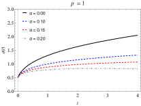
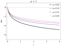
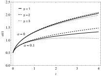
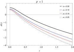
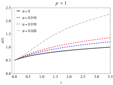
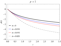
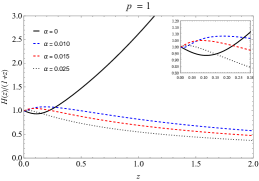
In the graphs of figures 1 and 2 the best values for $\alpha$ are between $0$ and $0.2$. Furthermore, in Fig 2 we can see the behavior of the functions $a(t)$ and $\phi(t)$ by varying the parameter $p$. Now, to solve the equations in terms of functions of the redshift $z$, where $z+1=1/a$ and

$$\dfrac{d}{dt}=-H(z+1)\dfrac{d}{dz},$$ (26)

the equation (22) and (23) become

$$3H^{2}(z) = H^{2}(z)(z+1)^{2}\left(\dfrac{1}{2}-\alpha\right)\dfrac{{\phi^{\prime}(z)}^{2}}{2}+\left(\dfrac{1}{2}+4\alpha\right)e^{2\phi}\phi^{p},$$

$$-2H(z)(1+z)H^{\prime}(z)+3H^{2}(z) = -H^{2}(z)(z+1)^{2}\left(\dfrac{1}{2}+3\alpha\right)\dfrac{{\phi^{\prime}(z)}^{2}}{2}+\left(\dfrac{1}{2}+4\alpha\right)e^{2\phi}\phi^{p},$$ (27)

where $(^{\prime})$ stands for derivative with respect to $z$. The deceleration parameter $q$ and the equation of state $\omega$ can be written as follows

$$q=-\left(1+\dfrac{\dot{H}}{H^{2}}\right),\qquad\omega=-\left(1+\dfrac{2\dot{H}}{3H^{2}}\right).$$ (28)

Considering the following initial conditions $H_{0}=H(z=0)=1$, $\phi^{\prime}_{0}=\dfrac{d\phi}{dz}\Big{|}_{z=0}=10^{-2}$, for the initial condition of $\phi_{0}=\phi(z=0)$ we solve the following equation

$$\dfrac{12-(1-2\alpha)\phi^{\prime}_{0}}{2(1+8\alpha)}=e^{2\phi_{0}}\phi_{0}^{p}.$$ (29)

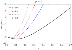
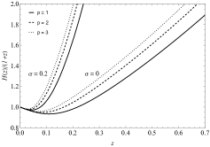
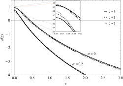
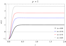
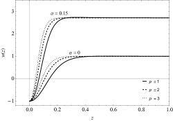
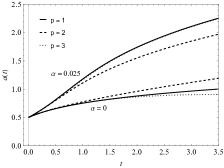
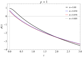
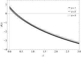
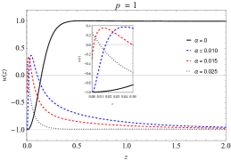
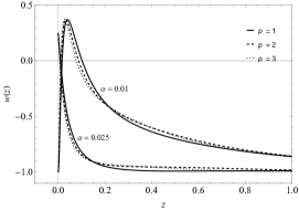
The numerical solutions to the equations in (27) using the mentioned initial conditions, for some values of $\alpha$ and $p$, are displayed in several graphs. For instance, Fig. 3 and Fig. 3 display the Hubble parameter $H(z)$ and the scalar field $\phi(z)$ for several values of $\alpha$ and fixed $p$, whereas Fig 4 and Fig 4 show the behavior of $H(z)$ and $\phi(z)$ for two cases of $\alpha$ and $p=1,2,3$. In Fig. 5 and Fig. 5 we have the behavior of the equation of state $\omega$ for fixed $p$ and varying $\alpha$ and two fixed values of $\alpha$ and varying $p$, respectively.

Figure 3: Hubble parameter $H$ and the scalar field $\phi$ as functions of redshift $z$. We can see the influence of $\alpha$ on the behavior of the curves.

Figure 4: Behavior of the Hubble parameter $H$ and the scalar field $\phi$ for some values of $p$.

Figure 5: We have the equation of state $\omega$ as a function of redshift $z$. Notice the contribution of the parameter $\alpha$ on the behavior of the curves. In (b) we see the behavior of $\omega(z)$ for three values of $p$, in two different scenarios $\alpha=0$ and $\alpha=0.15$.

We can explore the parameters region that are in accord with some observational data. For instance, from Eq. (28) we can find the relationship between the equation of state $\omega(z)$ and the deceleration parameter $q(z)$ as follows

$$q=\frac{1}{2}(1+3\omega).$$ (30)

Now using the numerical plots for the equation of state in Fig. 5 at a redshift $z$ properly chosen, we can find values of the deceleration parameter $q(z)$ and make comparison with observational data. We summarize the results and discussions about this issue in the Table (1).

$q$	$\omega$	$\alpha$	$\rm curve$
$-0.71$	$-0.81$	$0$	${\color[rgb]{0,0,0}-\!\!\!-\!\!\!-}$
$-0.40$	$-0.60$	$0.10$	$\color[rgb]{0,0,1}---$
$-0.10$	$-0.40$	$0.15$	$\color[rgb]{1,0,0}---$
$+0.50$	$0.00$	$0.20$	$\color[rgb]{0,0,0}\cdot\cdot\cdot$

Table 1: The table shows the values of the decelerating parameter $q$ in terms of $\omega$ for several values of $\alpha$ and $p=1$ at $z\approx 0.05$ in Fig. 5. The values for $\alpha=0.10$ and $\alpha=0.15$ is consistent with supernovae observations that reveals $q(0)=-0.1\pm 0.4$ riess ; Riess:2016jrr , i.e. $q\in[-0.50,0.30]$.

IV.2 Model $f(R,T^{\phi})=R+\alpha\left(T^{\phi}\right)^{2}$

Let us now consider another explicit model of modified gravity and solve the following set of field equations

$$3H^{2} = \left(\dfrac{1}{2}+\alpha\dot{\phi}^{2}\right)\dfrac{\dot{\phi}^{2}}{2}+\left[\dfrac{1}{2}+8\alpha\left(3\tilde{V}(\phi)-\dot{\phi}^{2}\right)\right]\tilde{V}(\phi),$$

$$2\dot{H}+3H^{2} = -\left(\dfrac{1}{2}-5\alpha\dot{\phi}^{2}\right)\dfrac{\dot{\phi}^{2}}{2}+\left[\dfrac{1}{2}+8\alpha\left(3\tilde{V}(\phi)-2\dot{\phi}^{2}\right)\right]\tilde{V}(\phi).$$ (31)

We will use the same initial conditions as in the previous case to solve Eqs. (31). See that now the values of $\alpha$ chosen are much smaller than those used in the previous model. Several totally distinct scenarios between the present model and the previous model can been discussed according to the numerical results displayed in the corresponding graphs. The fact that this second model has a quadratic contribution of energy-momentum trace $T$, whereas this type of contribution is linear in the first model, translates into a phenomenon in which the first model favors late time accelerating cosmology, while the second model favors inflationary early Universe. For instance, the graphs in Fig. 1 and Fig. 6 responds inversely to the contribution of $T$ in approximately the same range of time, which confirms their opposite signatures of accelerating Universe in distinct asymptotic cosmological times. Another interesting behavior can be seen in Fig 10: all curves for the equation of state with the influence of $\alpha$ approach $-1$ for larger values of $z$. On the other hand, distinct results at $z$ close to zero can be seen with further details in the inset. In the figure 10 we can see the influence of the parameter $p$ in two different cases of $\alpha$. In the figure 8 we have the behavior of $H(z)$ using $p=1,\alpha=0.01$ to $0.025$ and $\phi(z)$ in Fig. 8. These same quantities, for different values of $p$, Fig. 9 and Fig. 9 show that the variation of the curves for values of $\alpha\neq 0$ are very small.

Figure 6: Behavior of solutions to the equation (31) as functions of time $t$. In $(a)$ evolution of $a(t)$ increases with increasing parameter $\alpha$. In $(b)$ we have a quicker decay of the scalar field $\phi$ with the increase of $\alpha$. In both quantities we have a considerable change in the behavior of the curve for $\alpha=0.025$.

Figure 7: Behavior of solutions to the equation (31) as functions of time $t$. In $(a)$ evolution of $a(t)$ splits into two distinct scenarios (for $p=2,3$) around the scenario with $p=1$. The splitting magnitude increases with parameter $\alpha$. In $(b)$ similar splitting of the scalar field $\phi$ is clearly observed with the increase of $\alpha$. Here differently of the previous model, for a larger $\alpha$ there are split scenarios degenerated with the case $p=1$.

Figure 8: Once again we have the behavior of the Hubble parameter $H$ and the scalar field $\phi$ as functions of the redshift $z$ for the second model. In the inset we have a zoom in close to $z=0$ and we can see the changes in the curves due to the presence of small $\alpha$.

Figure 9: Behavior of the Hubble parameter $H$ and the scalar field $\phi$ for some values of $p$. Notice the quantities, for different values of $p$ show that the variation of the curves for small values of $\alpha$ are very small.

Figure 10: We have the numerical result for the equation of state $\omega$ for a fixed $p$ (a) and varying $p$ (b). We can see that the behavior of the equation of state changes very strongly for small increases of the parameter $\alpha$.

V Conclusions

The study of two models of string theory inspired dilaton gravity in realm of modified $f(R,T)$ gravity show important diferences between them. The numerical analyses were made in both models and revealed in several cosmological quantities their fingerprints, i.e., they are mostly able to describe both dark energy and inflationary early Universe. In the first model that displays linear contributions in $T$ (trace of the energy-momentum tensor) seems to favor the well-accepted behavior of $\Lambda$-CDM model (the case $\alpha=0$) for low redshifts, which is in accord with the Planck 2018 data, whereas in quadratic contributions in $T$ displayed in the second model seems to develop opposite behavior of $\Lambda$-CDM model (the case $\alpha=0$) — this is specially noticed in the graphs for $H(z)$. It is interesting to notice that from Fig. 4 at $z=0.2$ the values chosen for the parameters $\alpha$ and $p$ allow to possibly sweep all the well-accepted values of $H_{0}$ Riess:2016jrr . On the other hand, as we check the equation of state $\omega(z)$ of the second model it looks that is describing a transition from negative values at late (dark energy regime) and early (inflationary regime) presenting positive values (radiation and matter regimes) in between. Another interesting example is the behaviour of the curves for $p=1$ and $\alpha=0.025$ in Fig. 10 (inset) and Fig. 10, and Fig. 8 (inset) and Fig. 9 (inset) for large $z$ in complete agreement with inflationary regime depicted in Fig. 6 and Fig. 7 in early Universe. In this case one could apply several investigations on the inflationary regime such as constraining the parameters through contour plot in the plane made out of scalar spectral indices and tensor-to-scalar ratio Santos:2017alg ; Santos:2023zob . Further studies following the lines of Brito:2005zw ; Bazeia:2007vx ; Barosi:2008gx ; Santos:2019ljs ; Neves:2020anh ; SantosdaCosta:2020dyl with different models in dilatonic $f(R,T)$ gravity should be addressed elsewhere.

References

- (1) A. G. Riess et al., Astron. J. 116, 1009 (1998). S. Perlmutter et al., Astrophys. J. 517, 565 (1999).
- (2) T. Koivisto, D.F. Mota, Phys. Rev. D 73, 083502 (2006). S.F. Daniel, Phys. Rev. D 77, 103513 (2008).
- (3) C.L. Bennett et al., Astrophys. J. Suppl. 148, 119-134 (2003). D.N. Spergel et al., [WMAP Collaboration], Astrophys. J. Suppl. 148, 175 (2003). G. Hinshaw et al., Astrophys. J. Suppl. 208, 19 (2013).
- (4) R.R. Caldwell, M. Doran, Phys. Rev. D 69, 103517 (2004). Z.Y. Huang et al., JCAP 0605, 013 (2006).
- (5) D.J. Eisenstein et al., Astrophys. J. 633, 560 (2005). W.J. Percival at el., Mon. Not. R. Astron. Soc. 401, 2148(2010).
- (6) B. P. Abbott et al. (LIGO Scientific Collaboration and Virgo Collaboration), Observation of Gravitational Waves from a Binary Black Hole Merger, Phys. Rev. Lett. 116, 061102 (2016)
- (7) T. Padmanabhan, “Dark energy and gravity,” Gen. Rel. Grav. 40 (2008) 529–564.
- (8) J. Frieman, M. Turner, and D. Huterer, “Dark Energy and the Accelerating Universe,” Ann. Rev. Astron. Astrophys. 46 (2008) 385–432.
- (9) J. Martin, “Quintessence: a mini-review,” Mod. Phys. Lett. A 23 (2008) 1252–1265.
- (10) R. R. Caldwell and M. Kamionkowski, “The Physics of Cosmic Acceleration,” Ann. Rev. Nucl. Part. Sci. 59 (2009) 397–429.
- (11) A. Silvestri and M. Trodden, “Approaches to Understanding Cosmic Acceleration,” Rept. Prog. Phys. 72 (2009) 096901.
- (12) K. Bamba, S. Capozziello, S. Nojiri, and S. D. Odintsov, “Dark energy cosmology: the equivalent description via different theoretical models and cosmography tests,” Astrophys. Space Sci. 342 (2012) 155–228.
- (13) M. Li, X.-D. Li, S. Wang, and Y. Wang, “Dark Energy: A Brief Review,” Front. Phys. (Beijing) 8 (2013) 828–846.
- (14) M. Sami and R. Myrzakulov, “Late time cosmic acceleration: ABCD of dark energy and modified theories of gravity,” Int. J. Mod. Phys. D 25 no. 12, (2016) 1630031].
- (15) P. J. E. Peebles and B. Ratra, “The Cosmological Constant and Dark Energy,” Rev. Mod. Phys. 75 (2003) 559–606.
- (16) T. Padmanabhan, “Cosmological constant: The Weight of the vacuum,” Phys. Rept. 380 (2003) 235–320.
- (17) V. Sahni, “The Cosmological constant problem and quintessence,” Class. Quant. Grav. 19 (2002) 3435–3448.
- (18) H. E. S. Velten, R. F. Vom Marttens, W Zimdahl, The Eur.Phys. J. C. 74, 3160, (2014)
- (19) Shinji Tsujikawa. Quintessence: A Review. Class. Quant. Grav., 30:214003, 2013.
- (20) Buchdahl, H. A. (1970). ”Non-linear Lagrangians and cosmological theory”. Monthly Notices of the Royal Astronomical Society. 150: 1–8.
- (21) T.P. Sotiriou and V. Faraoni, theories of gravity, Rev. Mod. Phys. 82 (2010) 451.
- (22) Starobinsky, A. A. (1980). ”A new type of isotropic cosmological models without singularity”. Physics Letters B. 91 (1): 99–102.
- (23) Carroll, S M, Duvvuri, V, Trodden, M. Turner, M S “Is cosmic speed-up due to new gravitational physics ?”, Phys. Rev. D70 (2004), 043528.
- (24) Capozziello, S, Cardone, V F, Carloni, S. Troisi, A “Curvature quintessence matched with observational data”, Int. J. Mod. Phys. D12 (2003), 1969-1982.
- (25) V. Dzhunushaliev at al., Modified gravity from the quantum part of the metric, Eur. Phys. J. C 74, 2743 (2014). R. Yang, Effects of quantum fluctuations of metric on the universe, Physics of the Dark Universe 13, 87 (2016). X. Liu, T. Harko and SD. Liang, Cosmological implications of modified gravity induced by quantum metric fluctuations, Eur. Phys. J. C 76, 420 (2016).
- (26) T. Harko et al., Phys. Rev. D 84, 024020 (2011).
- (27) H. Shabani and M. Farhoudi, cosmological models in phase space, Phys. Rev. D 88, 044048 (2013).
- (28) Min-Xing Xu, T. Harko, and Shi-Dong Liang, Quantum Cosmology of gravity, Eur. Phys. J. C 76, 449 (2016).
- (29) P. H. R. S. Moraes and P. K. Sahoo, The simplest non-minimal matter-geometry coupling in the cosmology, Eur. Phys. J. C 77, 480 (2017).
- (30) H. Shabani and A. H. Ziaie, Bouncing cosmological solutions from gravity, Eur. Phys. J. C 78, 397 (2018).
- (31) P. S. Debnath, Bulk viscous cosmological model in theory of gravity, Int. J.Geom. Meth. Mod. Phys. 16, 1950005 (2019).
- (32) S. Bhattacharjee and P. Sahoo, Comprehensive analysis of a non-singular bounce in gravitation, Physics of the Dark Universe 28, 100537 (2020).
- (33) S. Bhattacharjee et al., Inflation in gravity, Eur. Phys. J. Plus 135, 576 (2020).
- (34) M. Gamonal, Slow-roll inflation in gravity and a modified Starobinsky-like inflationary model, Physics of the Dark Universe 31, 100768 (2021).
- (35) E. Witten, Phys. Lett. B149 (1984) 351.
- (36) E. Witten, Nucl. Phys. B443 (1995) 85.
- (37) M. Gasperini, Phys. Rev. D64 (2001) 043510; M. Gasperini, F. Piazza and G. Veneziano, Phys. Rev. D65 (2001) 023508.
- (38) G. Veneziano. Large N bounds on, and compositeness limit of, gauge and gravitational interactions. JHEP 06 (2002) 051.
- (39) A. G. Riess et al. [Supernova Search Team], Observational evidence from supernovae for an accelerating universe and a cosmological constant, Astron. J. 116, 1009 (1998) doi:10.1086/300499 [astro-ph/9805201].
- (40) A. G. Riess, L. M. Macri, S. L. Hoffmann, D. Scolnic, S. Casertano, A. V. Filippenko, B. E. Tucker, M. J. Reid, D. O. Jones and J. M. Silverman, et al. A 2.4% Determination of the Local Value of the Hubble Constant, Astrophys. J. 826, no.1, 56 (2016) doi:10.3847/0004-637X/826/1/56 [arXiv:1604.01424 [astro-ph.CO]].
- (41) M. A. Santos, M. Benetti, J. Alcaniz, F. A. Brito and R. Silva, CMB constraints on -exponential inflationary models, JCAP 03, 023 (2018) doi:10.1088/1475-7516/2018/03/023 [arXiv:1710.09808 [astro-ph.CO]].
- (42) J. R. L. Santos, S. S. da Costa and R. S. Santos, Cosmological models for f(R,T)() gravity, Phys. Dark Univ. 42, 101356 (2023) doi:10.1016/j.dark.2023.101356
- (43) F. A. Brito, F. F. Cruz and J. F. N. Oliveira, Accelerating universes driven by bulk particles, Phys. Rev. D 71, 083516 (2005) doi:10.1103/PhysRevD.71.083516 [arXiv:hep-th/0502057 [hep-th]].
- (44) L. Barosi, F. A. Brito and A. R. Queiroz, Noncommutative field gas driven inflation, JCAP 04, 005 (2008) doi:10.1088/1475-7516/2008/04/005 [arXiv:0801.0810 [hep-th]].
- (45) D. Bazeia, F. A. Brito and F. G. Costa, First-order framework and domain-wall/brane-cosmology correspondence, Phys. Lett. B 661, 179-185 (2008) doi:10.1016/j.physletb.2008.02.016 [arXiv:0707.0680 [hep-th]].
- (46) F. F. Santos, R. M. P. Neves and F. A. Brito, Modeling dark sector in Horndeski gravity at first-order formalism, Adv. High Energy Phys. 2019, 3486805 (2019) doi:10.1155/2019/3486805 [arXiv:1906.11821 [hep-th]].
- (47) R. M. P. Neves, S. Santos Da Costa, F. A. Brito and J. S. Alcaniz, Brane inflation driven by an arctan potential: CMB constraints and reheating, JCAP 07, no.07, 024 (2022) doi:10.1088/1475-7516/2022/07/024 [arXiv:2011.05264 [hep-th]].
- (48) S. Santos da Costa, M. Benetti, R. M. P. Neves, F. A. Brito, R. Silva and J. S. Alcaniz, Brane inflation and the robustness of the Starobinsky inflationary model, Eur. Phys. J. Plus 136, no.1, 84 (2021) doi:10.1140/epjp/s13360-020-01015-1 [arXiv:2007.09211 [astro-ph.CO]].