Data augmentation for the POD formulation of the parametric laminar incompressible Navier-Stokes equations

Abstract

A posteriori reduced-order models, e.g. proper orthogonal decomposition, are essential to affordably tackle realistic parametric problems. They rely on a trustful training set, that is a family of full-order solutions (snapshots) representative of all possible outcomes of the parametric problem. Having such a rich collection of snapshots is not, in many cases, computationally viable. A strategy for data augmentation, designed for parametric laminar incompressible flows, is proposed to enrich poorly populated training sets. The goal is to include in the new, artificial snapshots emerging features, not present in the original basis, that do enhance the quality of the reduced-order solution. The methodologies devised are based on exploiting basic physical principles, such as mass and momentum conservation, to devise physically-relevant, artificial snapshots at a fraction of the cost of additional full-order solutions. Interestingly, the numerical results show that the ideas exploiting only mass conservation (i.e., incompressibility) are not producing significant added value with respect to the standard linear combinations of snapshots. Conversely, accounting for the linearized momentum balance via the Oseen equation does improve the quality of the resulting approximation and therefore is an effective data augmentation strategy in the framework of viscous incompressible laminar flows.

Keywords: Reduced-order models, Proper orthogonal decomposition, Data augmentation, Incompressible Navier-Stokes, Scientific machine learning.

1 Introduction

Reduced-Order Models (ROM) are commonly employed to construct affordable solutions of multi-query, parametric problems (Chinesta et al., 2017; Peherstorfer et al., 2018). Although well established, the techniques to devise ROMs might face computational bottlenecks, when the underlying physical models are nonlinear (Carlberg et al., 2011, 2013; Nguyen and Peraire, 2023), the space of parameters is high dimensional (Bui-Thanh et al., 2008; Constantine, 2015) and the cost of each simulation is expensive, like in computational fluid dynamics applications, see, e.g., Mengaldo et al. (2021) and Löhner et al. (2021). Indeed, the issues mentioned above are particularly critical when parametric incompressible flows are considered, from laminar (Stabile and Rozza, 2018; Tsiolakis et al., 2020), to turbulent (Hijazi et al., 2020; Ahmed et al., 2021; Tsiolakis et al., 2022) regimes, in the context of parameterized geometries (Ballarin et al., 2016; Giacomini et al., 2021) or uncertain inputs (Musharbash and Nobile, 2018; Piazzola et al., 2023). Whilst such challenges are especially relevant in transient, turbulent flows, many conceptual difficulties already arise in steady, laminar flows, and the present work focuses on the parametric incompressible Navier-Stokes equations at low and moderate Reynolds number.

To construct a surrogate model for such parametric flow problems, a posteriori ROMs rely on collecting a family of snapshots (corresponding to different instances of the parameters) and using them as a basis to describe a reduced space where the solution is sought (Burkardt et al., 2006; Patera and Rozza, 2007; Rozza et al., 2008; Nguyen and Peraire, 2008; Wang et al., 2012). It is worth noticing that the set of snapshots, the training set, has to be representative of the full space of solutions, and this generally entails a large number of high-fidelity solutions, and a high computational cost. Possible redundancies in the training set typically yield ill-conditioned reduced-order problems. These redundancies are however readily suppressed using Proper Orthogonal Decomposition (POD).

In an effort to reduce the amount of required snapshots, adaptive sampling and dimensionality reduction techniques of the input space were proposed, see e.g., Bui-Thanh et al. (2008) and Raghavan et al. (2013). More recently, alternative approaches to make the construction of ROMs computationally affordable relied on multi-fidelity strategies mixing simulations on different levels of mesh refinement in the physical and parametric space (Ng and Willcox, 2014; Xiao et al., 2018; Jakeman et al., 2022) and domain decomposition techniques to couple local ROMs computed on smaller subdomains (Barnett et al., 2022; Discacciati and Hesthaven, 2023; Discacciati et al., 2024).

Although effective, all the above-mentioned strategies entail the solution of a certain number of full-order problems to populate the training set. This work proposes to further reduce the computational investment needed to generate the training set by producing artificial snapshots and augmenting data in the context of parametric viscous laminar incompressible flows. The idea stems from the work in Díez et al. (2021), where a strategy to expand the training set by adding new elements, artificially generated from the original snapshots with simple algebraic operations, was proposed. Of course, these artificial snapshots are meaningful if they enrich the approximation space, providing better approximations to new solutions of the parametric problem. The present contribution bypasses the simple framework of a parametric linear convection-diffusion equation to treat the more complex setting of the steady incompressible Navier-Stokes equations. In this context, more sophisticated strategies are necessary to create new training solutions combining the original snapshots, while accounting for the underlying physics of the problem under analysis. More precisely, physics-informed strategies exploiting mass and momentum conservation principles are employed for data augmentation, yielding new, physically-relevant, artificial snapshots at a fraction of the cost of additional full-order solutions. Finally, recall that augmenting the training set is never counterproductive (POD suppresses redundancies) and it can be extremely useful if the new elements bring pieces of information that are absent in the original set and pertinent to capture features of new parametric solutions.

The remainder of the paper is structured as follows. Section 2 describes the problem statement, introduces notation and the standard strategy to solve the full-order model. Then, in Section 3, the basics of POD are briefly recollected, together with its application in the context of mixed formulations of nonlinear problems. Section 4 devises the proposed methodologies to augment the data and enrich the training set, accounting for the physical knowledge of the problem under analysis. Numerical examples, presented in Section 5, demonstrate the suitability of the discussed approaches to augment the training set with physically-relevant information, enhancing the achievements of the POD-ROM approximation. Finally, concluding remarks are collected in Section 6.

2 Full-order model: steady incompressible Navier-Stokes equations

In this Section, the full-order model of the problem under analysis, the steady laminar incompressible Navier-Stokes equations, is recalled and the high-fidelity solver employed for the computation of the snapshots is introduced.

2.1 Problem statement

The problem under consideration consists in finding a velocity field $u$ and a pressure field $p$ taking values in $\Omega\subset\leavevmode\hbox{$\rm I\!R$}^{d}$ (the space dimension $d$ is equal to 2 or 3), and such that

$$\left\{\begin{aligned} -\text{\boldmath$\nabla$\unboldmath}\cdot\left(\nu\text{\boldmath$\nabla$\unboldmath}\text{\boldmath$u$\unboldmath}-p\text{\boldmath$I$\unboldmath}\right)+\left(\text{\boldmath$u$\unboldmath}\cdot\text{\boldmath$\nabla$\unboldmath}\right)\text{\boldmath$u$\unboldmath}&=\text{\boldmath$0$\unboldmath}&\text{in }\Omega,\\ \text{\boldmath$\nabla$\unboldmath}\cdot\text{\boldmath$u$\unboldmath}&=0&\text{in }\Omega,\\ \text{\boldmath$u$\unboldmath}&=\text{\boldmath$u$\unboldmath}_{D}&\text{on }\Gamma_{D},\\ \left(\nu\text{\boldmath$\nabla$\unboldmath}\text{\boldmath$u$\unboldmath}-p\text{\boldmath$I$\unboldmath}\right)\text{\boldmath$n$\unboldmath}&=\text{\boldmath$t$\unboldmath}&\text{on }\Gamma_{N},\end{aligned}\right.$$ (1)

where $\nu>0$ is the kinematic viscosity, $\text{\boldmath$u$\unboldmath}_{D}$ the velocity prescribed on $\Gamma_{D}$, $t$ the pseudo-traction prescribed on $\Gamma_{N}$, $I$ stands for the $d\times d$ identity matrix, and $n$ is the outward unit normal to the boundary. The two parts $\Gamma_{D}$ and $\Gamma_{N}$ of the boundary $\partial\Omega$, where Dirichlet and Neumann boundary conditions are enforced, are such that $\partial\Omega={\bar{\Gamma}_{D}}\cup{\bar{\Gamma}_{N}}$, and $\Gamma_{D}\cap\Gamma_{N}=\emptyset$.

Problem (1) is considered to be parametric in the sense that the input data (and therefore the solution $(\text{\boldmath$u$\unboldmath},p)$) depend on ${n_{p}}$ parameters collected in a vector $\text{\boldmath$\mu$\unboldmath}\in\leavevmode\hbox{$\rm I\!R$}^{n_{p}}$. These parameters may affect material properties of the fluid ($\nu$), working conditions ($\text{\boldmath$u$\unboldmath}_{D}$, $t$), the geometry of the domain or the parts of the boundary where the boundary conditions are enforced.

The corresponding weak form is derived using weighted residual technique and reads: find $(\text{\boldmath$u$\unboldmath},p)\in[H^{1}(\Omega)]^{d}\times L^{2}(\Omega)$ such that $\text{\boldmath$u$\unboldmath}=\text{\boldmath$u$\unboldmath}_{D}$ on $\Gamma_{D}$ and

$$\left\{\begin{aligned} d(\text{\boldmath$u$\unboldmath},\text{\boldmath$v$\unboldmath})+c(\text{\boldmath$u$\unboldmath},\text{\boldmath$u$\unboldmath},\text{\boldmath$v$\unboldmath})-b(\text{\boldmath$v$\unboldmath},p)&=\int_{\Gamma_{N}}\text{\boldmath$t$\unboldmath}\cdot\text{\boldmath$v$\unboldmath}\,d\Gamma,\\ b(\text{\boldmath$u$\unboldmath},q)&=0,\end{aligned}\right.$$ (2)

for every $\text{\boldmath$v$\unboldmath}\in[H^{1}_{0}(\Omega)]^{d}=\{\text{\boldmath$v$\unboldmath}\in[H^{1}(\Omega)]^{d}:\text{\boldmath$v$\unboldmath}|_{\Gamma_{D}}=\text{\boldmath$0$\unboldmath}\}$ and for every $q\in L^{2}(\Omega)$. The forms in (2) are

$$d(\text{\boldmath$u$\unboldmath},\text{\boldmath$v$\unboldmath}) =\int_{\Omega}\nu\,\text{\boldmath$\nabla$\unboldmath}\text{\boldmath$u$\unboldmath}:\text{\boldmath$\nabla$\unboldmath}\text{\boldmath$v$\unboldmath}\,\textnormal{d}\Omega,$$ (3)

$$c(\text{\boldmath$w$\unboldmath},\text{\boldmath$u$\unboldmath},\text{\boldmath$v$\unboldmath}) =\int_{\Omega}\left(\text{\boldmath$w$\unboldmath}\cdot\text{\boldmath$\nabla$\unboldmath}\text{\boldmath$u$\unboldmath}\right)\cdot\text{\boldmath$v$\unboldmath}\,\textnormal{d}\Omega,$$

$$b(\text{\boldmath$v$\unboldmath},q) =\int_{\Omega}q\,\text{\boldmath$\nabla$\unboldmath}\cdot\text{\boldmath$v$\unboldmath}\,\textnormal{d}\Omega.$$

In practice, one possibility to deal with inhomogeneous Dirichlet conditions ($\text{\boldmath$u$\unboldmath}_{D}\neq\text{\boldmath$0$\unboldmath}$) is taking $\text{\boldmath$u$\unboldmath}=\text{\boldmath$u$\unboldmath}_{0}+\text{\boldmath$r$\unboldmath}_{g}$, $\text{\boldmath$r$\unboldmath}_{g}$ being a lift function such that $\text{\boldmath$r$\unboldmath}_{g}|_{\Gamma_{D}}=\text{\boldmath$u$\unboldmath}_{D}$. Thus, the actual unknown is such that $\text{\boldmath$u$\unboldmath}_{0}|_{\Gamma_{D}}=\text{\boldmath$0$\unboldmath}$ and belongs to the same space as $v$.

Note that problem (1) is nonlinear and therefore is to be solved iteratively. Next Section briefly describes the formulation of the Newton-Raphson method employed within the high-fidelity solver in this work.

2.2 Newton-Raphson iteration

An iterative scheme is devised to numerically solve problem (1) (or the equivalent weak form (2)). Given some approximation $(\text{\boldmath$u$\unboldmath}^{k},p^{k})$, for $k=0,1,\dots$ ($k$ is the iteration counter), the subsequent iteration $(\text{\boldmath$u$\unboldmath}^{k+1},p^{k+1})$ is characterized by increments $(\delta{\text{\boldmath$u$\unboldmath}},\delta p)$ such that $\text{\boldmath$u$\unboldmath}^{k+1}=\text{\boldmath$u$\unboldmath}^{k}+\delta{\text{\boldmath$u$\unboldmath}}$ and $p^{k+1}=p^{k}+\delta p$.

Thus, introducing the $\text{\boldmath$u$\unboldmath}=\text{\boldmath$u$\unboldmath}^{k}+\delta{\text{\boldmath$u$\unboldmath}}$ and $p=p^{k}+\delta p$ in (2) results in the following linearized equation for the unknown $(\text{\boldmath$u$\unboldmath},p)$,

$$\left\{\begin{aligned} d(\delta{\text{\boldmath$u$\unboldmath}},\text{\boldmath$v$\unboldmath})+c(\text{\boldmath$u$\unboldmath}^{k},\delta{\text{\boldmath$u$\unboldmath}},\text{\boldmath$v$\unboldmath})+c(\delta{\text{\boldmath$u$\unboldmath}},\text{\boldmath$u$\unboldmath}^{k},\text{\boldmath$v$\unboldmath})-b(\text{\boldmath$v$\unboldmath},\delta p)&=\int_{\Gamma_{N}}\text{\boldmath$t$\unboldmath}\cdot\text{\boldmath$v$\unboldmath}\,d\Gamma\\ &\,\,\,\,\,-d(\text{\boldmath$u$\unboldmath}^{k},\text{\boldmath$v$\unboldmath})\\ &\,\,\,\,\,-c(\text{\boldmath$u$\unboldmath}^{k},\text{\boldmath$u$\unboldmath}^{k},\text{\boldmath$v$\unboldmath})\\ &\,\,\,\,\,+b(\text{\boldmath$v$\unboldmath},p^{k}),\\ b(\delta{\text{\boldmath$u$\unboldmath}},q)&=-b(\text{\boldmath$u$\unboldmath}^{k},q).\end{aligned}\right.$$ (4)

Note that the term $c(\delta{\text{\boldmath$u$\unboldmath}},\delta{\text{\boldmath$u$\unboldmath}},\text{\boldmath$v$\unboldmath})$ features a second-order increment, thus it is considered to be negligible and drops out in (4).

It is assumed that $\text{\boldmath$u$\unboldmath}^{k}$ fulfils the Dirichlet boundary conditions, therefore $\delta{\text{\boldmath$u$\unboldmath}}$ is enforced to satisfy their homogeneous counterpart.

The linear problem (4) characterising every iteration is discretized with a standard finite element approach. Namely, the velocity field $\text{\boldmath$u$\unboldmath}^{k}$ is represented by the vector of nodal values ${\textbf{u}}^{k}\in\leavevmode\hbox{$\rm I\!R$}^{\texttt{n}^{\!u}}$, and the pressure field $p^{k}$ is represented, in its discrete form, by the vector ${\textbf{p}}^{k}\in\leavevmode\hbox{$\rm I\!R$}^{\texttt{n}^{p}}$ ($\texttt{n}^{\!u}$ and $\texttt{n}^{p}$ are the number of degrees of freedom in the velocity and pressure discretizations), such that

$$\text{\boldmath$u$\unboldmath}^{k}=\sum_{i=1}^{\texttt{n}^{\!u}}[{\textbf{u}}^{k}]_{i}\text{\boldmath$N$\unboldmath}^{u}_{i}\quad\text{ and }\quad p^{k}=\sum_{i=1}^{\texttt{n}^{p}}[{\textbf{p}}^{k}]_{i}{N}^{p}_{i},$$ (5)

$\text{\boldmath$N$\unboldmath}^{u}_{i}$ and ${N}^{p}_{i}$, being the shape functions corresponding to the $i$-th degree of freedom of velocity and pressure, respectively. Henceforth, a finite element pair for velocity and pressure fulfilling the inf-sup or LBB condition, e.g., the Taylor-Hood elements, is assumed (Donea and Huerta, 2003; Quarteroni and Valli, 2008). Analogously, the vectors of nodal values describing $\delta{\text{\boldmath$u$\unboldmath}}$ and $\delta p$ read $\delta$u and $\delta$p. We are aware the difference of notation between the fields and the vectors of nodal values representing them is somehow subtle. Nevertheless, we firmly believe the reader will distinguish them easily due to the context.

The matrices representing the discrete counterparts of the operators introduced in (3), in the discrete spaces spanned by the finite element basis functions $\text{\boldmath$N$\unboldmath}^{u}_{i}$ (for $i=1,2,\dots,\texttt{n}^{\!u}$) and ${N}^{p}_{i}$ (for $i=1,2,\dots,\texttt{n}^{p}$), are

$$\text{\boldmath$D$\unboldmath}\in\leavevmode\hbox{$\rm I\!R$}^{\texttt{n}^{\!u}\times\texttt{n}^{\!u}} [\text{\boldmath$D$\unboldmath}]_{ij} =d(\text{\boldmath$N$\unboldmath}^{u}_{i},\text{\boldmath$N$\unboldmath}^{u}_{j}),$$ with generic term

$$\text{\boldmath$C$\unboldmath}_{1}(\text{\boldmath$u$\unboldmath}^{k})\in\leavevmode\hbox{$\rm I\!R$}^{\texttt{n}^{\!u}\times\texttt{n}^{\!u}} [\text{\boldmath$C$\unboldmath}_{1}(\text{\boldmath$u$\unboldmath}^{k})]_{ij} =c(\text{\boldmath$u$\unboldmath}^{k},\text{\boldmath$N$\unboldmath}^{u}_{j},\text{\boldmath$N$\unboldmath}^{u}_{i}),$$ with generic term

$$\text{\boldmath$C$\unboldmath}_{2}(\text{\boldmath$u$\unboldmath}^{k})\in\leavevmode\hbox{$\rm I\!R$}^{\texttt{n}^{\!u}\times\texttt{n}^{\!u}} [\text{\boldmath$C$\unboldmath}_{2}(\text{\boldmath$u$\unboldmath}^{k})]_{ij} =c(\text{\boldmath$N$\unboldmath}^{u}_{j},\text{\boldmath$u$\unboldmath}^{k},\text{\boldmath$N$\unboldmath}^{u}_{i}),$$ with generic term

$$\text{\boldmath$B$\unboldmath}\in\leavevmode\hbox{$\rm I\!R$}^{\texttt{n}^{p}\times\texttt{n}^{\!u}} [\text{\boldmath$B$\unboldmath}]_{ij} =b(\text{\boldmath$N$\unboldmath}^{u}_{j},{N}^{p}_{i}).$$ with generic term

Thus, the discrete version of (4) results in the following linear algebraic system:

$$\begin{bmatrix}\text{\boldmath$D$\unboldmath}+\text{\boldmath$C$\unboldmath}_{1}(\text{\boldmath$u$\unboldmath}^{k})+\text{\boldmath$C$\unboldmath}_{2}(\text{\boldmath$u$\unboldmath}^{k})&\text{\boldmath$B$\unboldmath}^{\textsf{T}}\\ \text{\boldmath$B$\unboldmath}&\text{\boldmath$0$\unboldmath}\end{bmatrix}\begin{bmatrix}{\text{\boldmath$\delta$\unboldmath}\!\textbf{u}}\\ {\text{\boldmath$\delta$\unboldmath}\!\textbf{p}}\end{bmatrix}=\begin{bmatrix}{\textbf{f}}-\text{\boldmath$D$\unboldmath}{\textbf{u}}^{k}-\text{\boldmath$C$\unboldmath}_{1}(\text{\boldmath$u$\unboldmath}^{k}){\textbf{u}}^{k}-\text{\boldmath$B$\unboldmath}^{\textsf{T}}{\textbf{p}}^{k}\\ -\text{\boldmath$B$\unboldmath}\text{\boldmath$u$\unboldmath}^{k}\end{bmatrix},$$ (6)

where f is the discrete version of the Neumann term in (4), that is,

$$[{\textbf{f}}\,]_{i}=\int_{\Gamma_{N}}\text{\boldmath$t$\unboldmath}\cdot\text{\boldmath$N$\unboldmath}^{u}_{i}\,d\Gamma\,,\quad\text{ for }i=1,2,\dots,\texttt{n}^{\!u}\,.$$

Thus, system (6) is to be solved at each iteration. Both the matrix and the right-hand-side term depend on the input parameters of the system (the parameters $\mu$ mentioned above) and on the previous iteration $(\text{\boldmath$u$\unboldmath}^{k},p^{k})$. The need of solving many systems corresponding to slightly different parametric entries suggests the use of ROMs.

3 Reduced-order model: Proper Orthogonal Decomposition

In this Section, the main ideas of the standard Proper Orthogonal Decomposition formulation are briefly summarized, with special emphasis towards the construction of a stable POD-ROM for incompressible flows (Veroy and Patera, 2005; Rozza and Veroy, 2007; Ballarin et al., 2015; Stabile and Rozza, 2018).

3.1 POD for linear systems of equations

Consider the general case in which the parametric unknown ${\textbf{x}}(\text{\boldmath$\mu$\unboldmath})$ is a vector of dimension $\texttt{n}^{x}$ obtained as the solution of the linear system of equations

$$\text{\boldmath$K$\unboldmath}(\text{\boldmath$\mu$\unboldmath}){\textbf{x}}(\text{\boldmath$\mu$\unboldmath})=\text{\boldmath$f$\unboldmath}(\text{\boldmath$\mu$\unboldmath}),$$ (7)

where, with respect to the previous Section, x plays the role of $\delta$u and $\delta$p.

Let ${\texttt{n}_{\texttt{S}}}$ be the number of snapshots ${\textbf{x}}_{i}$, for $i=1,\dots,{\texttt{n}_{\texttt{S}}}$ corresponding to high-fidelity solutions of the full-order problem (7) for ${\texttt{n}_{\texttt{S}}}$ values of the input parameters $\mu$. The snapshots are centred and collected in the matrix $X$ such that

$$\text{\boldmath$X$\unboldmath}=\left[\widehat{{\textbf{x}}}_{1}\,\,\widehat{{\textbf{x}}}_{2}\,\,\dots\,\,\widehat{{\textbf{x}}}_{{\texttt{n}_{\texttt{S}}}}\right],\text{ where }\widehat{{\textbf{x}}}_{i}={{\textbf{x}}}_{i}-\bar{{\textbf{x}}}\text{ and }\bar{{\textbf{x}}}=\dfrac{1}{{\texttt{n}_{\texttt{S}}}}\sum_{i=1}^{{\texttt{n}_{\texttt{S}}}}{{\textbf{x}}}_{i}.$$ (8)

The Principal Component Analysis, which is based on the Singular Value Decomposition (SVD), is used to eliminate redundancies in $X$. The SVD of $X$ reads

$$\text{\boldmath$X$\unboldmath}=\text{\boldmath$U$\unboldmath}\text{\boldmath$\Sigma$\unboldmath}\text{\boldmath$V$\unboldmath}^{\textsf{T}},$$ (9)

where $\text{\boldmath$\Sigma$\unboldmath}\in\leavevmode\hbox{$\rm I\!R$}^{\texttt{n}^{x}\times{\texttt{n}_{\texttt{S}}}}$ is a diagonal matrix containing the singular values of $X$ in descending order, $\sigma_{1}\geq\sigma_{2}\geq\dots\geq\sigma_{\texttt{n}_{\texttt{S}}}\geq 0$.

The first ${\texttt{n}_{\texttt{S}}}$ columns of $U$ define an orthonormal basis for the linear subspace generated by the snapshots. The more relevant information is contained in the first ones, which correspond to larger singular values. In practice, selecting a tolerance $\varepsilon$, the first ${\texttt{n}_{\texttt{POD}}}$ columns of $U$ are kept, ${\texttt{n}_{\texttt{POD}}}$ being such that

$$\sum_{i=1}^{\texttt{n}_{\texttt{POD}}}\sigma_{i}\geq(1-\varepsilon)\sum_{i=1}^{{\texttt{n}_{\texttt{S}}}}\sigma_{i}.$$ (10)

The POD consists in representing the unknown x in terms of only these ${\texttt{n}_{\texttt{POD}}}$ modes (${\texttt{n}_{\texttt{POD}}}$ is expected to be much lower than ${\texttt{n}_{\texttt{S}}}$, and ${\texttt{n}_{\texttt{S}}}$ is typically taken much lower than the dimension of the full-order system). Namely,

$${\textbf{x}}\simeq\bar{\textbf{x}}+\text{\boldmath$U$\unboldmath}^{\star}\text{\boldmath$z$\unboldmath}=\bar{\textbf{x}}+\sum_{i=1}^{\texttt{n}_{\texttt{POD}}}[\text{\boldmath$U$\unboldmath}]_{i}z_{i},$$ (11)

where $\text{\boldmath$z$\unboldmath}=[z_{1}\,z_{2}\dots z_{\texttt{n}_{\texttt{S}}}]^{\top}$ is the vector of the POD unknowns, and $\text{\boldmath$U$\unboldmath}^{\star}$ is the matrix containing the first ${\texttt{n}_{\texttt{POD}}}$ columns of $U$. Thus, the full-order system (7) can be readily reduced to

$$[\text{\boldmath$U$\unboldmath}^{\star\top}\text{\boldmath$K$\unboldmath}(\text{\boldmath$\mu$\unboldmath})\text{\boldmath$U$\unboldmath}^{\star}]\,\text{\boldmath$z$\unboldmath}=\text{\boldmath$U$\unboldmath}^{\star\top}\text{\boldmath$f$\unboldmath}(\text{\boldmath$\mu$\unboldmath})-\text{\boldmath$U$\unboldmath}^{\star\top}\text{\boldmath$K$\unboldmath}(\text{\boldmath$\mu$\unboldmath})\,\bar{\textbf{x}},$$ (12)

which is the reduced POD system of size ${\texttt{n}_{\texttt{POD}}}$.

3.2 POD for Navier-Stokes iterations

As mentioned in Section 3.1, ${\texttt{n}_{\texttt{S}}}$ snapshots are collected as solutions of the discrete version of the full-order problem (2) corresponding to different values of the input parameters $\mu$, that is the solution of (6) upon convergence of the Newton-Raphson iterations.

Two snapshot matrices $\text{\boldmath$X$\unboldmath}_{\!u}$ and $\text{\boldmath$X$\unboldmath}_{\!p}$ are thus collected separately for velocity and pressure. Following the POD strategy described above, the SVD applied to $\text{\boldmath$X$\unboldmath}_{\!u}$ and $\text{\boldmath$X$\unboldmath}_{\!p}$ provides truncated bases $\text{\boldmath$U$\unboldmath}_{\!\!u}^{\star}$ and $\text{\boldmath$U$\unboldmath}_{\!\!p}^{\star}$, being ${\texttt{n}_{\texttt{POD}}^{u}}$ and ${\texttt{n}_{\texttt{POD}}^{p}}$ the number of terms kept for each approximation. Note that the tolerance $\varepsilon$ used in (10) to set the number of terms may be different for velocity and pressure.

It follows that the unknowns $\delta$u and $\delta$p are approximated as

$${\text{\boldmath$\delta$\unboldmath}\!\textbf{u}}\simeq\text{\boldmath$U$\unboldmath}_{\!\!u}^{\star}\text{\boldmath$z$\unboldmath}_{u}\quad\text{ and }\quad{\text{\boldmath$\delta$\unboldmath}\!\textbf{p}}\simeq\text{\boldmath$U$\unboldmath}_{\!\!p}^{\star}\text{\boldmath$z$\unboldmath}_{p},$$ (13)

where $\text{\boldmath$z$\unboldmath}_{u}$ and $\text{\boldmath$z$\unboldmath}_{p}$ are the reduced unknowns of size ${\texttt{n}_{\texttt{POD}}^{u}}$ and ${\texttt{n}_{\texttt{POD}}^{p}}$, respectively. In addition, the reduced version of the problem to be solved at each Newton-Raphson iteration is obtained pre-multiplying the equations in system (6) by $\text{\boldmath$U$\unboldmath}_{\!\!u}^{\star\,\top}$ and $\text{\boldmath$U$\unboldmath}_{\!\!p}^{\star\,\top}$, yielding

$$\begin{bmatrix}\text{\boldmath$K$\unboldmath}^{\star}&\text{\boldmath$B$\unboldmath}^{\star\top}\\ \text{\boldmath$B$\unboldmath}^{\star}&\text{\boldmath$0$\unboldmath}\end{bmatrix}\begin{bmatrix}\text{\boldmath$z$\unboldmath}_{u}\\ \text{\boldmath$z$\unboldmath}_{p}\end{bmatrix}=\begin{bmatrix}{\textbf{f}_{u}^{\,\star}}\\ {\textbf{f}_{p}^{\,\star}}\end{bmatrix},$$ (14a)

where the following matrices and vectors are introduced

$$\text{\boldmath$K$\unboldmath}^{\star} =\text{\boldmath$U$\unboldmath}_{\!\!u}^{\star\,\top}\left[\text{\boldmath$D$\unboldmath}+\text{\boldmath$C$\unboldmath}_{1}(\text{\boldmath$u$\unboldmath}^{k})+\text{\boldmath$C$\unboldmath}_{2}(\text{\boldmath$u$\unboldmath}^{k})\right]\text{\boldmath$U$\unboldmath}_{\!\!u}^{\star}\,,$$ (14b)

$$\text{\boldmath$B$\unboldmath}^{\star} =\text{\boldmath$U$\unboldmath}_{\!\!p}^{\star\,\top}\text{\boldmath$B$\unboldmath}\text{\boldmath$U$\unboldmath}_{\!\!u}^{\star}\,,$$ (14c)

$${\textbf{f}_{u}^{\,\star}} =\text{\boldmath$U$\unboldmath}_{\!\!u}^{\star\,\top}\left[{\textbf{f}}-\text{\boldmath$D$\unboldmath}{\textbf{u}}^{k}-\text{\boldmath$C$\unboldmath}_{1}(\text{\boldmath$u$\unboldmath}^{k}){\textbf{u}}^{k}-\text{\boldmath$B$\unboldmath}^{\textsf{T}}{\textbf{p}}^{k}\right]\,,$$ (14d)

$${\textbf{f}_{p}^{\,\star}} =-\text{\boldmath$U$\unboldmath}_{\!\!p}^{\star\,\top}\text{\boldmath$B$\unboldmath}\text{\boldmath$u$\unboldmath}^{k}\,.$$ (14e)

Note that the reduced system (14) maintains the saddle-point structure of the full-order approximation (6). It is well-known that, although the snapshots are computed using an LBB-compliant discretization, it is not guaranteed that the stability properties of the full-order system are preserved at the reduced level (Veroy and Patera, 2005; Rozza and Veroy, 2007; Gerner and Veroy, 2012).

In this context, one may also adopt a POD formulation of the saddle-point problem (14) with only a reduced approximation of velocity, avoiding to reconstruct the reduced pressure (see, e.g., Ito and Ravindran (1998); Veroy and Patera (2005); Gräßle et al. (2019)). Indeed, if all the elements in the velocity basis are weakly incompressible, any linear combination automatically preserves the solenoidal nature of the velocity and pressure, as a Lagrange multiplier to enforce incompressibility, is not required. Whilst, it is thus straightforward to guarantee incompressibility at the weak level when no-slip conditions are imposed on all the boundaries, the cases featuring inhomogeneous Dirichlet conditions (possibly depending upon the parameters $\mu$) or Neumann conditions are not so trivial. Under these assumptions, a linear combination of the snapshots, complemented with the Dirichlet boundary conditions, is not automatically solenoidal. Therefore, in order to enforce the incompressibility of the reduced-order approximation of velocity, a mixed formulation is required also at the reduced level, thus including pressure, as Lagrange multiplier to impose incompressibility, in equation (14).

3.3 Stability and pressure reconstruction

It is well-known that the pressure term is needed in many applications (Noack et al., 2005) and many quantities of engineering interest (e.g., aerodynamic forces, pressure drops, $\ldots$) require an assessment of the pressure field.

Nonetheless, as previously mentioned, the inf-sup stability of the full-order discretization does not imply the inf-sup stability of the reduced system. To achieve stable reduced approximations of pressure, different techniques have been proposed in the literature. On the one hand, the supremizer (Ballarin et al., 2015) and the Pressure Poisson Equation (Stabile and Rozza, 2018) introduce corrections either enriching the velocity space or performing a Helmholtz decomposition of the velocity, with the goal of obtaining a stable reduced system in the offline phase. On the other hand, stability can be retrieved in the online phase via pressure-stabilised Petrov-Galerkin strategies (Baiges et al., 2014; Caiazzo et al., 2014).

In this work, a two-step procedure inspired by the consideration that stable approximations for mixed formulations can be obtained selecting a discrete space for velocity richer enough with respect to the discrete space for pressure (Brezzi and Bathe, 1990; Chapelle and Bathe, 1993) is followed. First, the reduced basis for velocity is constructed setting two tolerances, $\varepsilon_{u}$ for $u$ and $\varepsilon_{p}$ for $p$, in the stopping criterion (10). To guarantee that the subspace generated by the reduced basis for velocity is more accurate than the one for pressure, $\varepsilon_{u}$ is selected lower than $\varepsilon_{p}$. Indeed, the reduced basis with low resolution selected for the pressure is sufficient to enforce the incompressible nature of the velocity but it does not provide an approximation of the pressure field with enough quality and physical significance. Hence, the second step of the procedure performs a simple post-process of the reduced velocity obtained with the POD to recover a physically consistent pressure field.

More precisely, note that the linear system to be solved at each iteration is a linearization of the nonlinear system

$$\begin{bmatrix}\text{\boldmath$K$\unboldmath}({\textbf{u}})&\text{\boldmath$B$\unboldmath}^{\textsf{T}}\\ \text{\boldmath$B$\unboldmath}&\text{\boldmath$0$\unboldmath}\end{bmatrix}\begin{bmatrix}{\textbf{u}}\\ {\textbf{p}}\end{bmatrix}=\begin{bmatrix}{\textbf{f}}\\ \text{\boldmath$0$\unboldmath}\end{bmatrix}.$$ (15)

Following the idea of velocity-pressure splitting (Temam, 2001; Gresho and Sani, 1987), the discretized momentum equation (i.e., the first row of (15))

$$\text{\boldmath$K$\unboldmath}({\textbf{u}})\,{\textbf{u}}+\text{\boldmath$B$\unboldmath}^{\top}{\textbf{p}}={\textbf{f}}$$ (16)

can be used to compute the pressure corresponding to the velocity field u. Thus, pre-multiplying (16) by $B$ yields to

$$\text{\boldmath$B$\unboldmath}\text{\boldmath$B$\unboldmath}^{\top}{\textbf{p}}=\text{\boldmath$B$\unboldmath}({\textbf{f}}-\text{\boldmath$K$\unboldmath}({\textbf{u}}){\textbf{u}}),$$ (17)

which is used as a simple post-process to recover the reduced pressure, one the reduced velocity is computed. Alternative strategies for pressure recovery within incompressible Navier-Stokes are analyzed in Kean and Schneier (2020).

4 Data augmentation

As previously mentioned, a bottleneck of the standard POD strategy is the necessity of having a sufficient number of snapshots, representative of the parametric family of solutions. Each snapshot is obtained solving a full-order problem, therefore it is demanding in terms of computational effort.

In Díez et al. (2021), a methodology was introduced to create new snapshots using simple operations upon the original ones and a priori knowledge of the physical behaviour of the solution. For convection-diffusion problems, the operation was simply a product of the solution fields (a Hadamard, component by component, product of the vectors of nodal values). This is a sensible choice in this context because the product of pulses that propagate and diffuse tends to create intermediate pulses, which are exactly the missing snapshots. The strategy of augmenting the family of snapshots with these new elements was denoted as quadratic enrichment.

Here, this idea of data augmentation is generalized by devising simple operations between the snapshots creating new functions that do likely approximate other snapshots, typically corresponding to intermediate parametric values.

4.1 Solenoidal field recovered from geometric average of stream functions

Consider two velocity snapshots $\text{\boldmath$u$\unboldmath}_{i}$ and $\text{\boldmath$u$\unboldmath}_{j}$, corresponding to parameters $\text{\boldmath$\mu$\unboldmath}_{i}$ and $\text{\boldmath$\mu$\unboldmath}_{j}$. The idea is to use them to easily compute a new velocity field $\text{\boldmath$u$\unboldmath}^{\star}$. Of course, the idea of taking the product of the two snapshots is readily discarded because this would break the solenoidal character of the solutions. Indeed, enforcing incompressibility is of outmost importance since this property describes the conservation of mass for the fluid under analysis. To achieve this, the velocity fields $\text{\boldmath$u$\unboldmath}_{i}$ and $\text{\boldmath$u$\unboldmath}_{j}$ are expressed in terms of the corresponding stream functions $\Psi_{i}$ and $\Psi_{j}$.

The stream functions $\Psi_{i}$ and $\Psi_{j}$ are thus geometrically averaged by computing a new stream function

$$\Psi^{\star}=(\Psi_{i})^{\alpha}(\Psi_{j})^{1-\alpha},$$ (18)

for a scalar weight $\alpha\in]0,1[$. Then, the velocity field $\text{\boldmath$u$\unboldmath}^{\star}$ corresponding to $\Psi^{\star}$ is an inexpensive, artificial snapshot, expected to be an approximation of the solution corresponding to some intermediate parameter, between $\text{\boldmath$\mu$\unboldmath}_{i}$ and $\text{\boldmath$\mu$\unboldmath}_{j}$.

Note that the operations of recovering $\Psi_{i}$ and $\Psi_{j}$ from $\text{\boldmath$u$\unboldmath}_{i}$ and $\text{\boldmath$u$\unboldmath}_{j}$ and then computing $\text{\boldmath$u$\unboldmath}^{\star}$ from $\Psi^{\star}$ are standard and computationally affordable. Indeed, in 2D, $\Psi_{i}$ is computed from $\text{\boldmath$u$\unboldmath}_{i}$ by solving the Poisson problem

$$\left\{\begin{aligned} -\text{\boldmath$\nabla$\unboldmath}^{2}\Psi_{i}&=\frac{\partial[\text{\boldmath$u$\unboldmath}_{i}]_{y}}{\partial x}-\frac{\partial[\text{\boldmath$u$\unboldmath}_{i}]_{x}}{\partial y}&\text{ in }\Omega,\\ \text{\boldmath$\nabla$\unboldmath}\Psi_{i}\cdot\text{\boldmath$n$\unboldmath}&=(-[\text{\boldmath$u$\unboldmath}_{i}]_{y},[\text{\boldmath$u$\unboldmath}_{i}]_{x})\cdot\text{\boldmath$n$\unboldmath}&\text{ on }\partial\Omega,\end{aligned}\right.$$ (19)

where $[\text{\boldmath$u$\unboldmath}_{i}]_{x}$ and $[\text{\boldmath$u$\unboldmath}_{i}]_{y}$ stand for the first and second components of $\text{\boldmath$u$\unboldmath}_{i}$, respectively. Note that only Neumann boundary conditions are set. Therefore, to have a unique solution, the value of $\Psi_{i}$ is to be set at some arbitrary point (e.g., $\Psi_{i}=0$ at a node lying on the boundary $\partial\Omega$). The velocity field $\text{\boldmath$u$\unboldmath}^{\star}$ corresponding to the new stream function $\Psi^{\star}$ is thus readily computed as

$$\text{\boldmath$u$\unboldmath}^{\star}=\begin{bmatrix}\,\,\,0&1\\ -1&0\end{bmatrix}\text{\boldmath$\nabla$\unboldmath}\Psi^{\star}.$$ (20)

Taking different values of $\alpha$ between 0 and 1, different intermediate velocity fields are generated from each pair of actual snapshots in the original training set.

As it is shown in the examples, in some cases the new snapshots generated with this technique are not bringing into the training set new pieces of information that contribute to improving the reduced-order solution. Surprisingly enough, the linear combination of the original snapshots inherent to the POD seems to contain the same information provided by the new snapshots obtained via an enrichment strategy enforcing only mass conservation. Thus, in order to further enrich the quality of the basis, a correction imposing momentum conservation via the Oseen equation is proposed.

4.2 Physics-informed enhancement using Oseen equation

Let $\text{\boldmath$u$\unboldmath}^{\star}$ be a new snapshot created following the strategy presented in Section 4.1. A new solution $\text{\boldmath$u$\unboldmath}^{\star\star}$ is computed as a post-process of $\text{\boldmath$u$\unboldmath}^{\star}$, to enhance its compliance with the physics of the problem via the fulfilment of the momentum equation.

The solenoidal field $\text{\boldmath$u$\unboldmath}^{\star}$ is used as input data for an Oseen problem, which is a linearization of the steady-state incompressible Navier-Stokes equation reading

$$\left\{\begin{aligned} -\text{\boldmath$\nabla$\unboldmath}\cdot\left(\nu\text{\boldmath$\nabla$\unboldmath}\text{\boldmath$u$\unboldmath}^{\star\star}-p\text{\boldmath$I$\unboldmath}\right)+\left(\text{\boldmath$u$\unboldmath}^{\star}\cdot\text{\boldmath$\nabla$\unboldmath}\right)\text{\boldmath$u$\unboldmath}^{\star\star}&=\text{\boldmath$0$\unboldmath}&\text{in }\Omega,\\ \text{\boldmath$\nabla$\unboldmath}\cdot\text{\boldmath$u$\unboldmath}^{\star\star}&=0&\text{in }\Omega,\end{aligned}\right.$$ (21)

complemented with the same type of boundary conditions as (1). In the case of boundary conditions which depend on the parameters of the problem $\mu$, an approximation of the corresponding value is to be inferred from $\text{\boldmath$u$\unboldmath}^{\star}$.

Note that the discrete form of (21) is a variation of (15), namely

$$\begin{bmatrix}\text{\boldmath$K$\unboldmath}({\textbf{u}}^{\star})&\text{\boldmath$B$\unboldmath}^{\textsf{T}}\\ \text{\boldmath$B$\unboldmath}&\text{\boldmath$0$\unboldmath}\end{bmatrix}\begin{bmatrix}{\textbf{u}}^{\star\star}\\ {\textbf{p}}\end{bmatrix}=\begin{bmatrix}{\textbf{f}}\\ \text{\boldmath$0$\unboldmath}\end{bmatrix},$$ (22)

with the peculiarity that the resulting problem (22) is linear. Of course, to construct the Oseen enhancement enforcing the momentum balance, this problem needs to be solved multiple times. Indeed, for each artificial snapshot $\text{\boldmath$u$\unboldmath}^{\star}$ created as solenoidal average of any pair of original snapshots, one problem (22) is to be solved. Although this might seem computationally demanding, only few terms in the matrix require to be updated when a new artificial snapshot is considered. In addition, exploiting the linearity of the resulting problem, efficient solution strategies can be devised using suitable Krylov subspace methods.

Remark 1.

An alternative enrichment strategy accounting for the momentum conservation principle can be devised by replacing the solenoidal average in (21) by a linear combination $\text{\boldmath$u$\unboldmath}^{\star}=\alpha\text{\boldmath$u$\unboldmath}_{i}+(1-\alpha)\text{\boldmath$u$\unboldmath}_{j}$ of the original snapshots $\text{\boldmath$u$\unboldmath}_{i}$ and $\text{\boldmath$u$\unboldmath}_{j}$, with a weighting coefficient $\alpha\in]0,1[$. Numerical examples comparing the two approaches are discussed in Section 5.

5 Numerical examples

In this Section, the presented data augmentation strategies are tested to construct artificial snapshots, within a POD approximation, for two benchmarks involving parametrized flow control problems, modeled by the steady-state incompressible Navier-Stokes equations.

Full-order simulations are performed using the open-source library FEniCS (Alnaes et al., 2015; Langtangen and Logg, 2017). In all computations, the tolerances for POD-based dimensionality reduction are set to $\varepsilon_{u}=10^{-3}$, for the velocity training set, and $\varepsilon_{p}=0.25$ for the pressure. Recall that the pressure is later reconstructed as a post-process of the POD velocity, as described in Section 3.3.

The three strategies discussed in Section 4 are tested to enrich the velocity training set, by incorporating artificial snapshots computed by:

1. solenoidal average of two snapshots (i.e., imposing mass conservation);

2. solenoidal average of two snapshots, enhanced with the Oseen equation (i.e., imposing mass and momentum conservation);

3. linear combination of two snapshots enhanced with the Oseen equation (i.e., imposing mass and momentum conservation).

For each strategy, the data augmentation procedure is performed with a weight coefficient $\alpha=0.1,0.2,\dots,0.9$ to construct $\text{\boldmath$u$\unboldmath}^{\star}$.

5.1 Jet control for flow past a cylinder

The first example, inspired by Rabault et al. (2019), consideres the flow past a cylinder where two blowing/sucking jets are introduced. Consider the domain $\Omega=[0,30.5]\times[0,16]\setminus\mathcal{B}_{0.5}(8,8)$, where $\mathcal{B}_{\mathrm{R}}(x_{c},y_{c})$ denotes the two-dimensional cylinder of radius $\mathrm{R}$ centered in $(x_{c},y_{c})$. The boundary $\partial\Omega$ is partitioned according to the schematics reported in Figure 1.

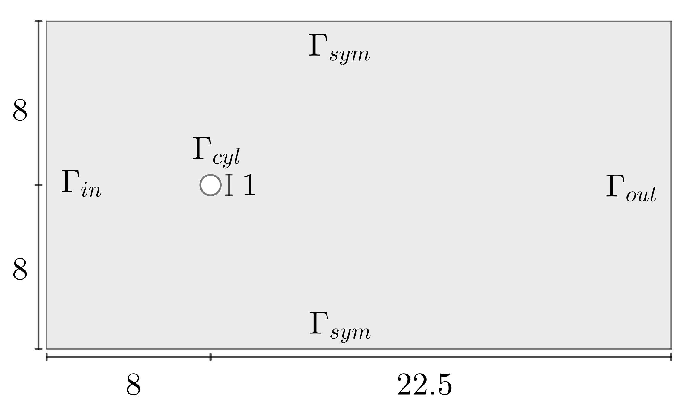
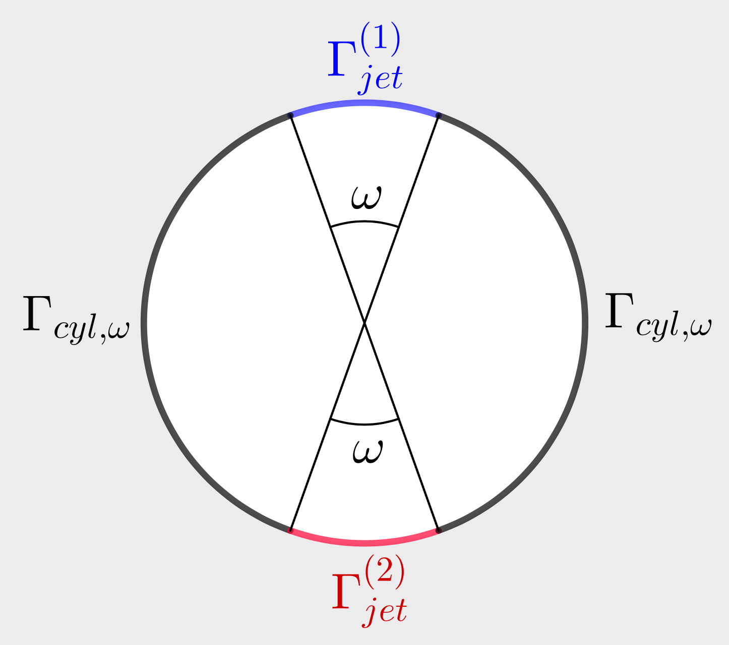
Figure 1: Geometry of the domain and boundary partition.

The fluid enters the domain with uniform horizontal velocity $\mathrm{U}_{\mathrm{in}}$ through the inlet on the left boundary, symmetry conditions are imposed on the top and bottom, and an outlet with homogeneous Neumann condition is added on the right vertical contour. On the surface of the cylinder, no-slip conditions are enforced, except for two portions, on the upper and lower parts, where two jets are inserted (Figure 1, right). The boundary conditions read

$$\text{\boldmath$u$\unboldmath} =[\mathrm{U}_{\mathrm{in}},0] \text{ on }\Gamma_{in},$$ (23a)

$$\text{\boldmath$u$\unboldmath}\cdot\text{\boldmath$n$\unboldmath} =0 \text{ on }\Gamma_{sym},$$

$$\text{\boldmath$\tau$\unboldmath}\cdot\left(\nu\text{\boldmath$\nabla$\unboldmath}\text{\boldmath$u$\unboldmath}-p\text{\boldmath$I$\unboldmath}\right)\text{\boldmath$n$\unboldmath} =0 \text{ on }\Gamma_{sym},$$

$$\text{\boldmath$u$\unboldmath} =\text{\boldmath$0$\unboldmath} \text{ on }\Gamma_{cyl,w},$$

$$\text{\boldmath$u$\unboldmath} =\gamma\mathbf{U}_{\!\mathrm{jet}} \text{ on }\Gamma_{jet}^{(1)},$$

$$\text{\boldmath$u$\unboldmath} =-\gamma\mathbf{U}_{\!\mathrm{jet}} \text{ on }\Gamma_{jet}^{(2)},$$

$$\left(\nu\text{\boldmath$\nabla$\unboldmath}\text{\boldmath$u$\unboldmath}-p\text{\boldmath$I$\unboldmath}\right)\text{\boldmath$n$\unboldmath} =\text{\boldmath$0$\unboldmath} \text{ on }\Gamma_{out},$$

where $$\tau \gamma$$ denotes the unit tangent vector, is a dimensionless parameter that modulates the maximum velocity of the jets, whereas their velocity profiles are given by

$$\mathbf{U}_{\!\mathrm{jet}}(x,y)=2\mathrm{U}_{\mathrm{in}}\cos\left(\frac{\pi}{\omega}\left(\theta-\frac{\pi}{2}\right)\right)\left[x-8,y-8\right],$$ (23b)

with $\omega=5\pi/36$ being the opening angle of each jet.

The kinematic viscosity is set to $\nu=0.01\textnormal{ m}^{2}/\textnormal{s}$ and the Reynolds number is ${\text{Re}}=\mathrm{U}_{\mathrm{in}}\mathrm{D}/\nu$, the characteristic length being the diameter $\mathrm{D}=1$ of the cylinder. The full-order solver relies on a $\mathbb{P}_{2}/\mathbb{P}_{1}$ finite element discretization computed on a mesh with $10,962$ triangular elements, suitably refined in the boundary layer region and in the wake of the cylinder. The resulting discretization features a total of $44,400$ degrees of freedom for velocity and $5,610$ for pressure.

The problem under analysis features two parameters: the Reynolds number ${\text{Re}}\in[5,30]$ (through the inlet velocity $\mathrm{U}_{\mathrm{in}}$) and the maximum velocity of the jets controlled by $\gamma\in[0,4]$. The velocity field for a representative set of solutions is shown in Figure 2.

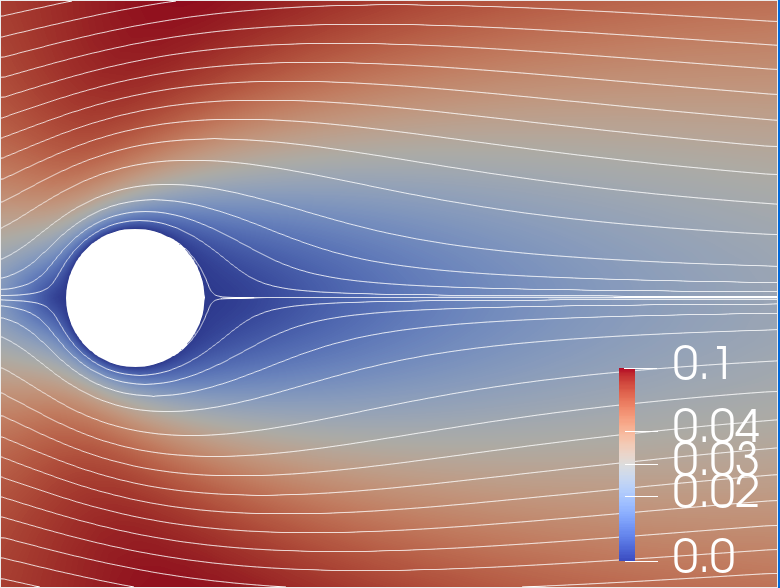
(a) ${\text{Re}}=5$, no jets ($\gamma=0$).

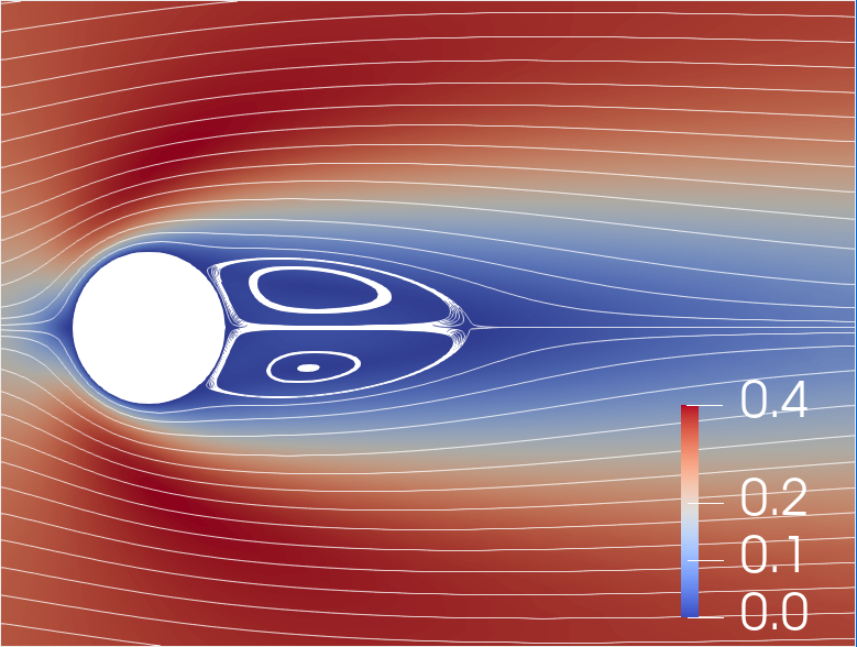
(b) ${\text{Re}}=30$, no jets ($\gamma=0$).

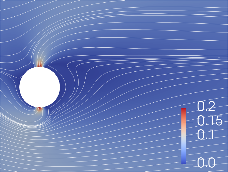
(c) ${\text{Re}}=5$, maximum jets ($\gamma=4$).

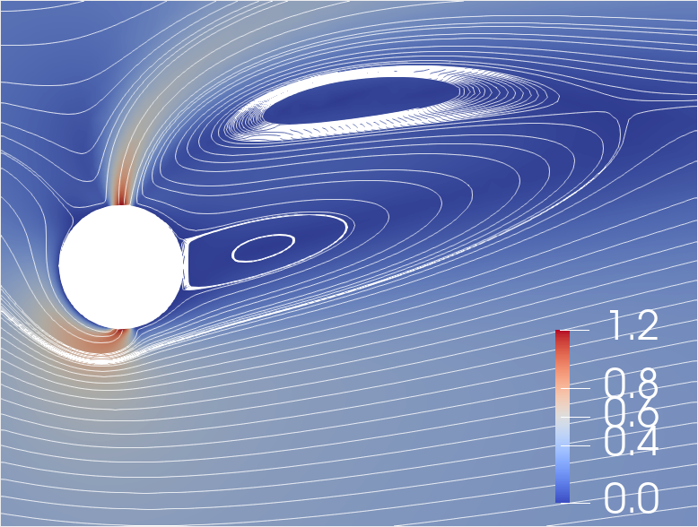
(d) ${\text{Re}}=30$ maximum jets ($\gamma=4$).

Figure 2: Velocity streamlines in the wake of the cylinder (area of interest $[7,13]\times[6,10]$) for representative values of the parameters ${\text{Re}}\in[5,30]$ and $\gamma\in[0,4]$ (jet velocity).

5.1.1 Single-parameter analysis

First, the proposed data augmentation strategies are analyzed in the case of a single parameter. Considering the parametrized Reynolds number Re, the value $\gamma=4$ is fixed. The original training set for the POD consists of only two snapshots, associated with ${\text{Re}}=5$ and ${\text{Re}}=30$. Upon augmentation, an enriched velocity training set of $11$ snapshots is obtained.

The reduced dimension for the pressure is ${\texttt{n}_{\texttt{POD}}^{p}}=1$. For the velocity, the reduced dimensions are ${\texttt{n}_{\texttt{POD}}^{u}}=1$ for the standard POD, ${\texttt{n}_{\texttt{POD}}^{u}}=3$ in the case of solenoidal averages enrichment, and ${\texttt{n}_{\texttt{POD}}^{u}}=4$ in the two cases with Oseen enhancement. The relative errors, measured in the Euclidean norm, of the reduced-order approximation at intermediate values of the Reynolds number are reported in Figure 3. In general, the results show that enriching the training set by means of solenoidal averages, that is, constructing artificial snapshots only enforcing mass conservation principle, does not improve the performance of POD. On the contrary, the physics-informed Oseen enhancement, in which both mass and momentum conservation are enforced, leads to more accurate solutions: errors improve for velocity, pressure, drag and lift in all tested values. For the velocity and pressure, the improvement is more significant for lower values of Re, around one order of magnitude, and is less pronounced as Re increases and the associated relative errors decrease. The same tendency on error evolution is observed for the lift. Regarding the drag, errors improve approximately one order of magnitude for all values of Re.

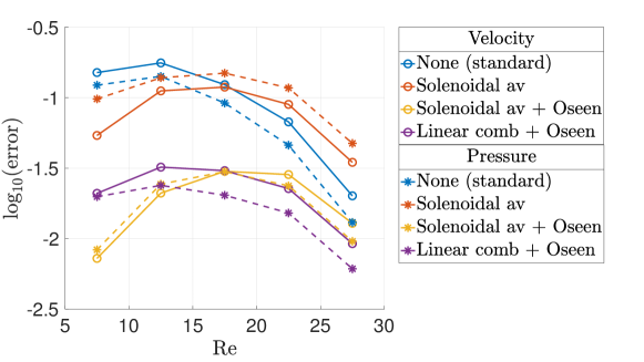
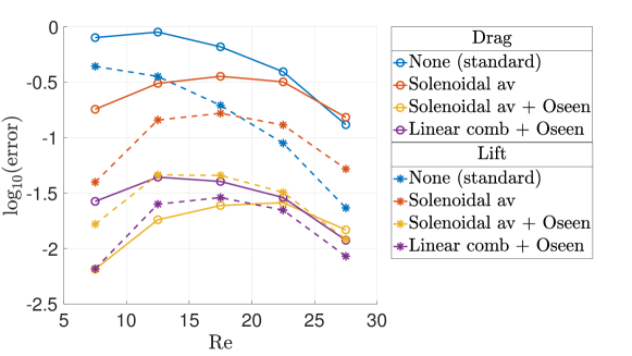
Figure 3: Relative errors, measured in the Euclidean norm, of velocity and pressure (top), drag and lift (bottom) for different strategies of data augmentation, with parametrized ${\text{Re}}\in[5,30]$ and fixed $\gamma=4$ .

The same tests is reproduced fixing ${\text{Re}}=30$ and considering $\gamma$ as unique parameter. As before, the training set consists of two snapshots, corresponding to $\gamma=0$ and $\gamma=4$, whereas the enriched velocity training set contains $11$ snapshots. It follows that the reduced dimensions are ${\texttt{n}_{\texttt{POD}}^{p}}=1$ for pressure, whereas for velocity the standard POD has a reduced space of dimension ${\texttt{n}_{\texttt{POD}}^{u}}=1$ which increases to ${\texttt{n}_{\texttt{POD}}^{u}}=4$ for the case of enrichment with solenoidal averages and ${\texttt{n}_{\texttt{POD}}^{u}}=6$ for the cases with Oseen enhancement. Figure 4 shows the relative errors at some intermediate values of $\gamma$, measured in the Euclidean norm. On the one hand, neglible differences are observed between the standard POD and the solenoidal averages enrichment strategy, highlighting that only imposing mass conservation during the construction of the artificial snapshots does not introduce relevant information not present in the original dataset. On the other hand, the Oseen enhancement is able to incorporate additional information, stemming from momentum conservation, into the approximation space and leads to more accurate results.

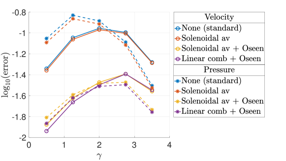
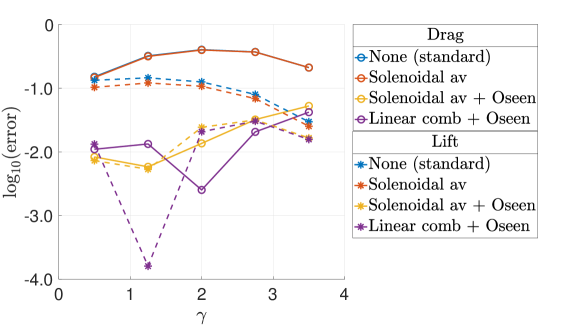
Figure 4: Relative errors, measured in the Euclidean norm, of velocity and pressure (top), drag and lift (bottom) for different strategies of data augmentation, with parametrized $\gamma\in[0,4]$ and fixed ${\text{Re}}=30$ .

Remark 2.

The two data augmentation approaches exploiting both mass and momentum conservation principles provide similar results in this example. Indeed, since the range of the Reynolds number under analysis is fairly low, all flows are highly viscous and vorticity effects are limited, whence both solenoidal averages and linear combinations of snapshots are able to provide sufficient information on the balance of forces. The performance of these two strategies in the context of transient problems and flows with more relevant vorticity effects should be thoroughly examined in future works.

5.1.2 Two-parameter analysis

Finally, the concurrent parametrization of Re and $\gamma$ is studied, with a training set comprising $25$ snapshots obtained from the uniform discretization of the parametric space. In particular, we consider the local POD approximation of the problem, accounting for the $5$ closest snapshots in the parametric space. Upon data augmentation, we include combinations of neighboring snapshots into the velocity training set, resulting into a collection of $59$ snapshots.

In Table 1, a comparison of the different enrichment techniques is presented. The dimension of the POD reduced spaces after data augmentation is reported, highlighting the capability of the proposed approaches to generate artificial snapshots.

Data	Dimension		Error
augmentation	${\texttt{n}_{\texttt{POD}}^{u}}$	${\texttt{n}_{\texttt{POD}}^{p}}$	Velocity	Pressure	Drag	Lift
None	$4$	$2$	$3.58\cdot 10^{-3}$	$6.48\cdot 10^{-3}$	$9.39\cdot 10^{-3}$	$2.06\cdot 10^{-3}$
(i)	$7$	$2$	$3.66\cdot 10^{-3}$	$6.36\cdot 10^{-3}$	$8.99\cdot 10^{-3}$	$4.63\cdot 10^{-3}$
(ii)	$8$	$2$	$5.97\cdot 10^{-4}$	$1.35\cdot 10^{-3}$	$3.07\cdot 10^{-4}$	$1.22\cdot 10^{-3}$
(iii)	$7$	$2$	$9.80\cdot 10^{-4}$	$1.60\cdot 10^{-3}$	$6.42\cdot 10^{-4}$	$1.92\cdot 10^{-3}$

Table 1: Relative errors, measured in the Euclidean norm, of the reduced-order approximation at ${\text{Re}}^{\star}=17.5$ and $\gamma^{\star}=1.5$ for different strategies of data augmentation: none, standard POD; (i) solenoidal average; (ii) solenoidal average with Oseen enhancement; (iii) linear combination with Oseen enhancement.

For a new point, corresponding to the parameters ${\text{Re}}^{\star}=17.5$ and $\gamma^{\star}=1.5$, not included in the training set, the relative errors of the reduced approximations, measured in the Euclidean norm, are also listed. The same behavior observed in the single-parameter analysis is confirmed in the case of two parameters. Data augmentation only enforcing mass conservation via solenoidal averages leads to similar approximation errors as the standard POD. On the contrary, accounting for both mass and momentum conservation by means of the Oseen enhancement strategy allows to significantly improve the errors for all the measured variables.

5.2 Lid-driven cavity with parametrized jets

In this Section, the test case of the lid-driven cavity with parametrized jets in Tsiolakis et al. (2020) is considered. In this problem, three jets are introduced into the classical non-leaky lid-driven cavity (Ghia et al., 1982). The spatial domain $\Omega=[0,1]^{2}$ is depicted in Figure 5.

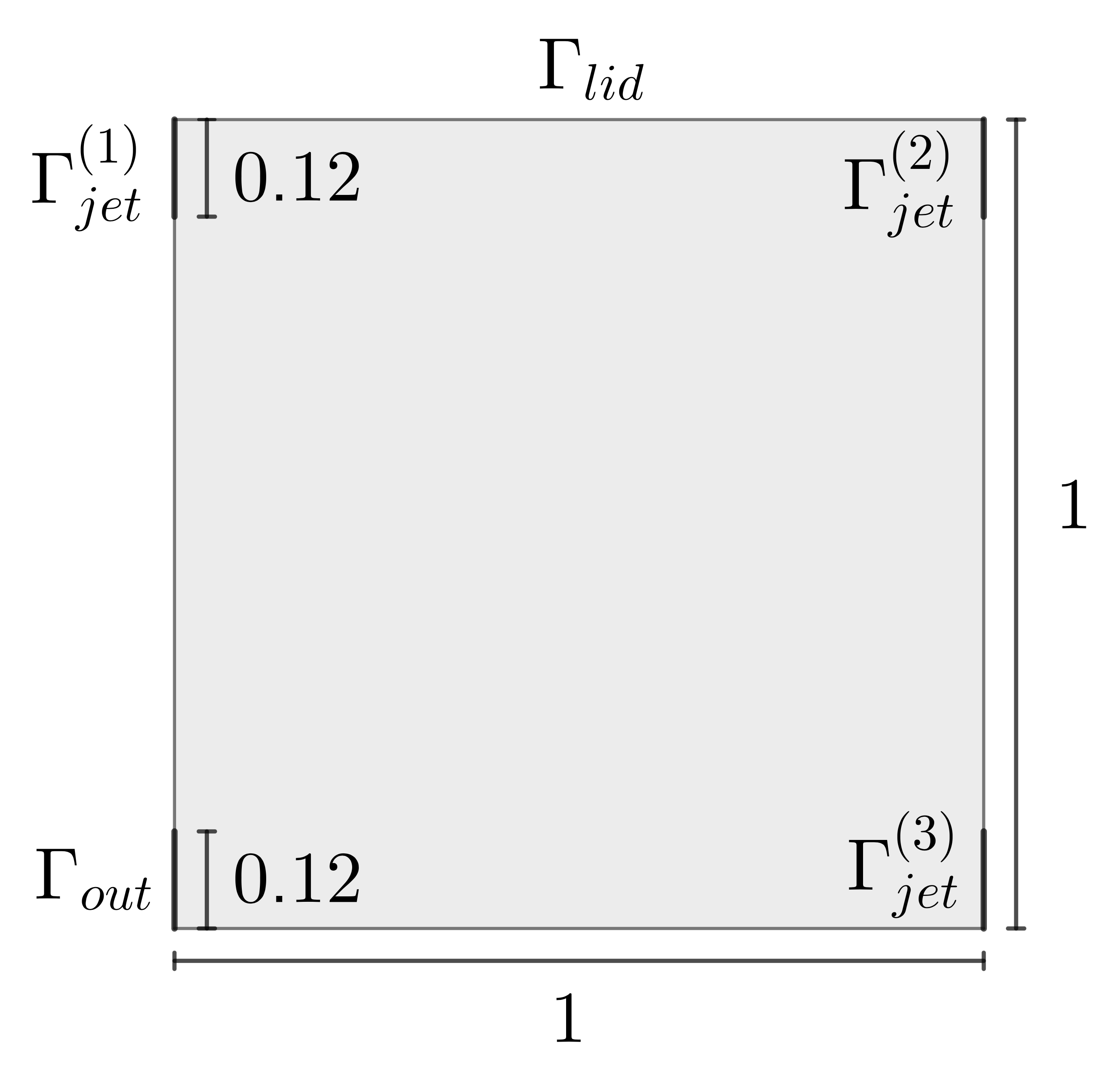
Figure 5: Geometry of the domain and boundary partition.

A horizontal velocity profile $\mathrm{U}_{\mathrm{lid}}(x)$ is imposed on the top lid of the domain, $\Gamma_{lid}$, and the three jets with horizontal velocity profiles $\mu\mathrm{U}_{\mathrm{jet}}^{(i)}(y)$ are introduced on the vertical walls at the locations defined by

$$\Gamma_{jet}^{(1)} =\{x=0,\ y\in[0.88,1]\}\,,$$ (24)

$$\Gamma_{jet}^{(2)} =\{x=1,\ y\in[0.88,1]\}\,,$$

$$\Gamma_{jet}^{(3)} =\{x=1,\ y\in[0,0.12]\}\,.$$

Moreover, an outlet surface is added on $\Gamma_{out}=\{x=0,\ y\in[0,0.12]\}$.

The complete set of imposed boundary conditions read

$$\text{\boldmath$u$\unboldmath} =[\mathrm{U}_{\mathrm{lid}},0] \textnormal{ on }\Gamma_{lid},$$ (25a)

$$\text{\boldmath$u$\unboldmath} =[\mu\mathrm{U}_{\mathrm{jet}}^{(i)},0] \textnormal{ on }\Gamma_{jet}^{(i)},\ i=1,\ldots,3,$$

$$\left(\nu\text{\boldmath$\nabla$\unboldmath}\text{\boldmath$u$\unboldmath}-p\text{\boldmath$I$\unboldmath}\right)\text{\boldmath$n$\unboldmath} =\text{\boldmath$0$\unboldmath} \textnormal{ on }\Gamma_{out},$$

$$\text{\boldmath$u$\unboldmath} =\text{\boldmath$0$\unboldmath} \textnormal{ elsewhere},$$

where the horizontal component of the lid velocity is given by

$$\mathrm{U}_{\mathrm{lid}}(x)=\begin{cases}10x/0.06&\textnormal{for }x\in[0,0.06],\\ 10&\textnormal{for }x\in(0.06,0.94),\\ 10(1-x)/0.06&\textnormal{for }x\in[0.94,1],\end{cases}$$ (25b)

whereas the profiles $$\mathrm{U}_{\mathrm{jet}}^{(i)} \Gamma_{jet}^{(i)},\ i=1,\ldots,3$$ on of the horizontal components of the jet velocities are defined as

$$\mathrm{U}_{\mathrm{jet}}^{(1)}(y) =1-\cos\left(2\pi(y-0.88)/0.12\right),$$ (25c)

$$\mathrm{U}_{\mathrm{jet}}^{(2)}(y) =1-\cos\left(2\pi(y-0.88)/0.12\right),$$

$$\mathrm{U}_{\mathrm{jet}}^{(3)}(y) =-1+\cos\left(2\pi y/0.12\right),$$

and scaled by the parameter $$\mu\in(0,1]$$.

The kinematic viscosity is set to $\nu=0.01\textnormal{ m}^{2}/\textnormal{s}$ and the resulting Reynolds number computed using $\max|\mathrm{U}_{\mathrm{lid}}|$ as characteristic velocity is ${\text{Re}}=1,000$. The high-fidelity solutions are computed using P2/P1 finite element basis on a mesh of $20,000$ triangular elements. The resulting discretization consists of $80,802$ degrees of freedom for velocity and $10,201$ for pressure.

The training set consists of two snapshots, corresponding to $\mu=0.05$ and $\mu=1$. The corresponding velocity fields and streamlines are displayed in Figure 6.

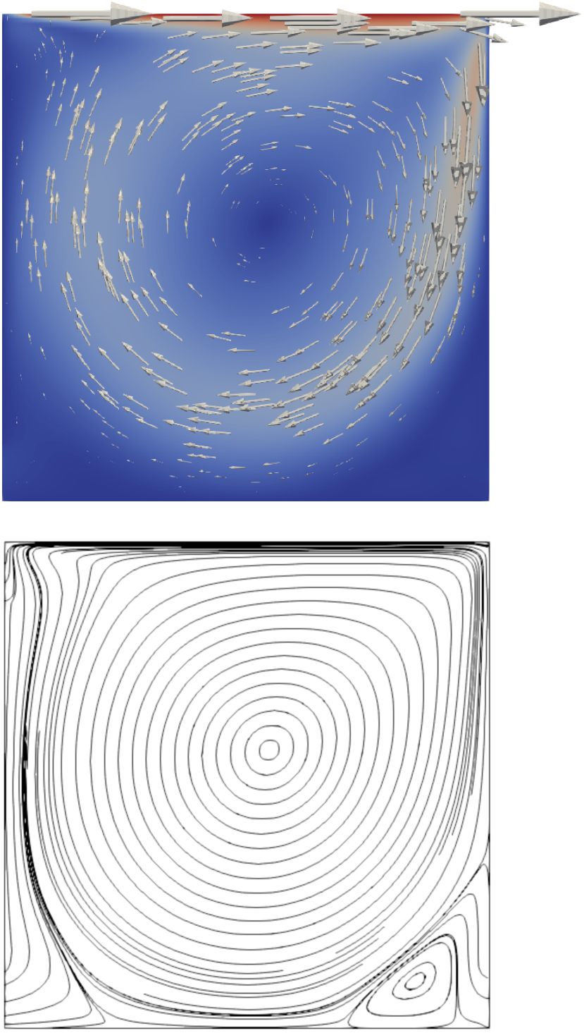
(a) $\mu=0.05$.

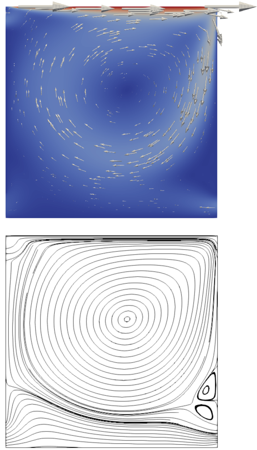
(b) $\mu=1$.

Figure 6: Velocity field (top) and velocity streamlines (bottom) for the two snapshots in the training set.

Upon enrichment, the augmented velocity training set contains $11$ elements.

Using all the proposed enriched datasets, the POD constructs reduced spaces of dimension ${\texttt{n}_{\texttt{POD}}^{u}}=5$ for velocity and ${\texttt{n}_{\texttt{POD}}^{p}}=1$ for pressure. For intermediate values of the parameter $\mu$, the solution is approximated by means of the standard POD and the proposed data augmentation strategies for the velocity. Table 2 lists the reduced dimensions and the relative errors, measured in the Euclidean norm, for the velocity and the pressure fields when approximating the solution for $\mu^{\star}=0.5$.

Data	Dimension		Error
augmentation	${\texttt{n}_{\texttt{POD}}^{u}}$	${\texttt{n}_{\texttt{POD}}^{p}}$	Velocity	Pressure
None	$1$	$1$	$5.12\cdot 10^{-2}$	$3.15\cdot 10^{-2}$
(i)	$5$	$1$	$5.13\cdot 10^{-2}$	$3.54\cdot 10^{-2}$
(ii)	$5$	$1$	$3.66\cdot 10^{-2}$	$4.09\cdot 10^{-2}$
(iii)	$5$	$1$	$3.38\cdot 10^{-2}$	$2.65\cdot 10^{-2}$

Table 2: Relative errors, measured in the Euclidean norm, of the reduced-order approximation at $\mu^{\star}=0.5$ for different strategies of data augmentation: none, standard POD; (i) solenoidal average; (ii) solenoidal average with Oseen enhancement; (iii) linear combination with Oseen enhancement.

For all the strategies, global errors comparable to the standard POD are achieved. However, incorporating the information about momentum conservation via the Oseen augmentation procedure provides richer artificial snapshots, capable of capturing detailed features of the solution. Indeed, Figure 7 displays the velocity streamlines for $\mu^{\star}=0.5$, highlighting the improved ability of the enriched dataset to capture local flow features, such as the nucleation or disappearance of vortices. In this case, the reference solution in Figure 7(a) shows a vortex in the left-bottom part of the domain. With the considered training set, the standard POD approximation is not able to capture the vortex (Figure 7(b)). Note that including the solenoidal averages to the training set (i.e., enforcing mass conservation in the artificial snapshots) does not provide sufficient additional information (Figure 7(c)). On the contrary, Figures 7(d) and 7(e) show that constructing artificial snapshots imposing both mass and momentum conservation principles via the Oseen correction, the reduced-order approximation is capable of identifying the appearence of a vortex where expected.

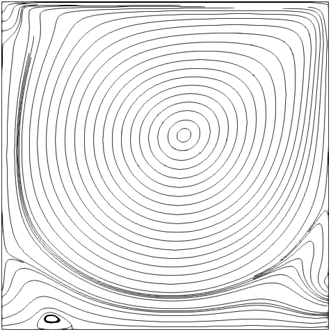
(a) High-fidelity solution.

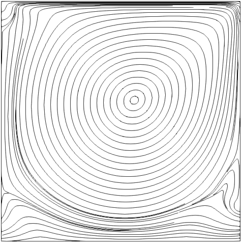
(b) Standard POD.

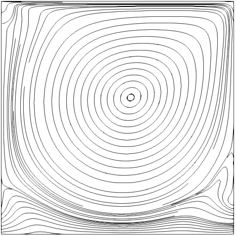
(c) Data augmentation (i).

  

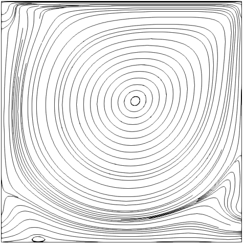
(d) Data augmentation (ii).

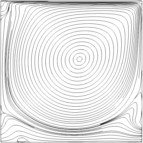
(e) Data augmentation (iii).

Figure 7: Velocity streamlines for $\mu^{\star}=0.5$ computed using (a) reference high-fidelity solver; (b) standard POD and data augmentation via (c) solenoidal average; (d) solenoidal average with Oseen enhancement; (e) linear combination with Oseen enhancement.

Similarly, the velocity streamlines for $\mu^{\star}=0.7$ are shown in Figure 8. In this case, the approximated solutions computed using standard POD and augmentation with solenoidal averages present two vortices on the bottom right region of the domain (Figures 8(b) and 8(c)), while only one is visible in the reference solution in Figure 8(a). The data augmentation relying on both mass and momentum conservation principles introduces in the training set artificial snapshots that improve the overall description of the flow and the reduced approximation displays patterns qualitatively more similar to the high-fidelity solution (Figures 8(d) and 8(e)).

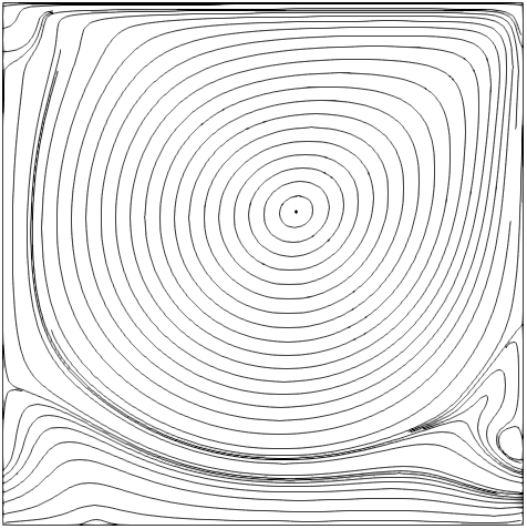
(a) High-fidelity solution.

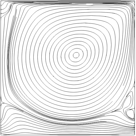
(b) Standard POD.

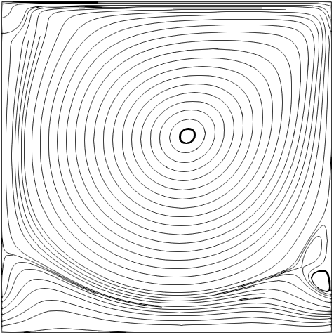
(c) Data augmentation (i).

  

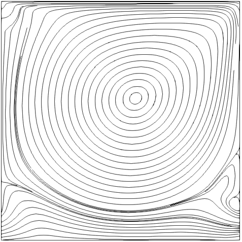
(d) Data augmentation (ii).

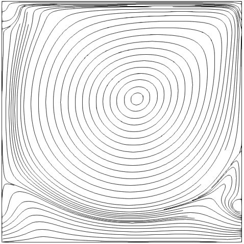
(e) Data augmentation (iii).

Figure 8: Velocity streamlines for $\mu^{\star}=0.7$ computed using (a) reference high-fidelity solver; (b) standard POD and data augmentation via (c) solenoidal average; (d) solenoidal average with Oseen enhancement; (e) linear combination with Oseen enhancement.

6 Concluding remarks

The methodologies presented in this paper aim at producing, with limited additional computational cost, new, artificial snapshots to enrich the training set for a posteriori ROMs. The ideas behind the proposed strategies are inspired in the physical knowledge of the solution, that is, enforcing mass and momentum conservation principles.

Two approaches are proposed, the one referred to as solenoidal geometric average constructs artificial snapshots fulfilling mass conservation equation, whereas the one labeled Oseen enhancement enforces both mass and momentum conservation. Despite the apparent soundness of the artificial snapshots produced by the solenoidal geometric average, it was found that, in the context of steady-state incompressible Navier-Stokes, they do not bring to the reduced basis gainful features. That is, no more than the linear combinations proposed by the standard POD computed using the original snapshots. On the contrary, accounting for both mass and momentum conservation principles via the Oseen enhancement is actually introducing in the training set new, relevant information, particularly useful to discover the features of parametric configurations not seen during the training procedure.

This opens the way to create data augmentation strategies, tailored for each specific application, to boost POD and related techniques. This is expected to release these ROMs from the computational burden of populating a training set with numerous full-order solutions. Of course, the suitability and performance of the proposed methodologies in the context of transient problems needs to be throroughly studied, assessing the individual relevance of mass and momentum conservation principles, when dynamic effects are involved.

References

- Ahmed et al. (2021) Ahmed, S.E., Pawar, S., San, O., Rasheed, A., Iliescu, T., Noack, B.R., 2021. On closures for reduced order models – A spectrum of first-principle to machine-learned avenues. Physics of Fluids 33, 091301.
- Alnaes et al. (2015) Alnaes, M.S., Blechta, J., Hake, J., Johansson, A., Kehlet, B., Logg, A., Richardson, C., Ring, J., Rognes, M.E., Wells, G.N., 2015. The FEniCS Project Version 1.5. Archive of Numerical Software 3.
- Baiges et al. (2014) Baiges, J., Codina, R., Idelsohn, S., 2014. Reduced-order modelling strategies for the finite element approximation of the incompressible Navier-Stokes equations, in: Idelsohn, S. (Ed.), Numerical Simulations of Coupled Problems in Engineering. Springer, pp. 189–216.
- Ballarin et al. (2016) Ballarin, F., Faggiano, E., Ippolito, S., Manzoni, A., Quarteroni, A., Rozza, G., Scrofani, R., 2016. Fast simulations of patient-specific haemodynamics of coronary artery bypass grafts based on a POD–Galerkin method and a vascular shape parametrization. Journal of Computational Physics 315, 609–628.
- Ballarin et al. (2015) Ballarin, F., Manzoni, A., Quarteroni, A., Rozza, G., 2015. Supremizer stabilization of POD–Galerkin approximation of parametrized steady incompressible Navier–Stokes equations. International Journal for Numerical Methods in Engineering 102, 1136–1161.
- Barnett et al. (2022) Barnett, J., Tezaur, I., Mota, A., 2022. The Schwarz alternating method for the seamless coupling of nonlinear reduced order models and full order models. Technical Report SAND2022-10280R. Computer Science Research Institute Summer Proceedings 2022, S.K. Seritan and J.D. Smith, eds., Sandia National Laboratories.
- Brezzi and Bathe (1990) Brezzi, F., Bathe, K.J., 1990. A discourse on the stability conditions for mixed finite element formulations. Computer Methods in Applied Mechanics and Engineering 82, 27–57.
- Bui-Thanh et al. (2008) Bui-Thanh, T., Willcox, K., Ghattas, O., 2008. Model reduction for large-scale systems with high-dimensional parametric input space. SIAM Journal on Scientific Computing 30, 3270–3288.
- Burkardt et al. (2006) Burkardt, J., Gunzburger, M., Lee, H.C., 2006. POD and CVT-based reduced-order modeling of Navier–Stokes flows. Computer Methods in Applied Mechanics and Engineering 196, 337–355.
- Caiazzo et al. (2014) Caiazzo, A., Iliescu, T., John, V., Schyschlowa, S., 2014. A numerical investigation of velocity–pressure reduced order models for incompressible flows. Journal of Computational Physics 259, 598–616.
- Carlberg et al. (2011) Carlberg, K., Bou-Mosleh, C., Farhat, C., 2011. Efficient non-linear model reduction via a least-squares Petrov–Galerkin projection and compressive tensor approximations. International Journal for Numerical Methods in Engineering 86, 155–181.
- Carlberg et al. (2013) Carlberg, K., Farhat, C., Cortial, J., Amsallem, D., 2013. The GNAT method for nonlinear model reduction: effective implementation and application to computational fluid dynamics and turbulent flows. Journal of Computational Physics 242, 623–647.
- Chapelle and Bathe (1993) Chapelle, D., Bathe, K.J., 1993. The inf-sup test. Computers & Structures 47, 537–545.
- Chinesta et al. (2017) Chinesta, F., Huerta, A., Rozza, G., Willcox, K., 2017. Model reduction methods, in: Encyclopedia of Computational Mechanics (Second Edition). Wiley & Sons, pp. 1–36.
- Constantine (2015) Constantine, P.G., 2015. Active subspaces: Emerging ideas for dimension reduction in parameter studies. SIAM.
- Díez et al. (2021) Díez, P., Muixí, A., Zlotnik, S., García-González, A., 2021. Nonlinear dimensionality reduction for parametric problems: a kernel Proper Orthogonal Decomposition (kPOD). International Journal for Numerical Methods in Engineering 122, 7306–7327.
- Discacciati et al. (2024) Discacciati, M., Evans, B.J., Giacomini, M., 2024. An overlapping domain decomposition method for the solution of parametric elliptic problems via proper generalized decomposition. Computer Methods in Applied Mechanics and Engineering 418, 116484.
- Discacciati and Hesthaven (2023) Discacciati, N., Hesthaven, J.S., 2023. Localized model order reduction and domain decomposition methods for coupled heterogeneous systems. International Journal for Numerical Methods in Engineering 124, 3964–3996.
- Donea and Huerta (2003) Donea, J., Huerta, A., 2003. Finite element methods for flow problems. John Wiley & Sons.
- Gerner and Veroy (2012) Gerner, A.L., Veroy, K., 2012. Certified reduced basis methods for parametrized saddle point problems. SIAM Journal on Scientific Computing 34, A2812–A2836.
- Ghia et al. (1982) Ghia, U., Ghia, K., Shin, C., 1982. High-Re solutions for incompressible flow using the Navier-Stokes equations and a multigrid method. Journal of Computational Physics 48, 387–411.
- Giacomini et al. (2021) Giacomini, M., Borchini, L., Sevilla, R., Huerta, A., 2021. Separated response surfaces for flows in parametrised domains: comparison of a priori and a posteriori PGD algorithms. Finite Elements in Analysis and Design 196, 103530.
- Gräßle et al. (2019) Gräßle, C., Hinze, M., Lang, J., Ullmann, S., 2019. POD model order reduction with space-adapted snapshots for incompressible flows. Advances in Computational Mathematics 45, 2401–2428.
- Gresho and Sani (1987) Gresho, P.M., Sani, R.L., 1987. On pressure boundary conditions for the incompressible Navier-Stokes equations. International Journal for Numerical Methods in Fluids 7, 1111–1145.
- Hijazi et al. (2020) Hijazi, S., Stabile, G., Mola, A., Rozza, G., 2020. Data-driven POD-Galerkin reduced order model for turbulent flows. Journal of Computational Physics 416, 109513.
- Ito and Ravindran (1998) Ito, K., Ravindran, S., 1998. A reduced-order method for simulation and control of fluid flows. Journal of Computational Physics 143, 403–425.
- Jakeman et al. (2022) Jakeman, J.D., Friedman, S., Eldred, M.S., Tamellini, L., Gorodetsky, A.A., Allaire, D., 2022. Adaptive experimental design for multi-fidelity surrogate modeling of multi-disciplinary systems. International Journal for Numerical Methods in Engineering 123, 2760–2790.
- Kean and Schneier (2020) Kean, K., Schneier, M., 2020. Error analysis of supremizer pressure recovery for POD based reduced-order models of the time-dependent Navier-Stokes equations. SIAM Journal on Numerical Analysis 58, 2235–2264.
- Langtangen and Logg (2017) Langtangen, H.P., Logg, A., 2017. Solving PDEs in Python. The FEniCS Tutorial. Springer.
- Löhner et al. (2021) Löhner, R., Othmer, C., Mrosek, M., Figueroa, A., Degro, A., 2021. Overnight industrial LES for external aerodynamics. Computers & Fluids 214, 104771.
- Mengaldo et al. (2021) Mengaldo, G., Moxey, D., Turner, M., Moura, R.C., Jassim, A., Taylor, M., Peiro, J., Sherwin, S., 2021. Industry-relevant implicit large-eddy simulation of a high-performance road car via spectral/hp element methods. SIAM Review 63, 723–755.
- Musharbash and Nobile (2018) Musharbash, E., Nobile, F., 2018. Dual dynamically orthogonal approximation of incompressible Navier Stokes equations with random boundary conditions. Journal of Computational Physics 354, 135–162.
- Ng and Willcox (2014) Ng, L.W., Willcox, K.E., 2014. Multifidelity approaches for optimization under uncertainty. International Journal for Numerical Methods in Engineering 100, 746–772.
- Nguyen and Peraire (2008) Nguyen, N.C., Peraire, J., 2008. An efficient reduced-order modeling approach for non-linear parametrized PDEs. International Journal for Numerical Methods in Engineering 76, 27 – 55.
- Nguyen and Peraire (2023) Nguyen, N.C., Peraire, J., 2023. Efficient and accurate nonlinear model reduction via first-order empirical interpolation. Journal of Computational Physics 494, 112512.
- Noack et al. (2005) Noack, B.R., Papas, P., Monkewitz, P.A., 2005. The need for a pressure-term representation in empirical Galerkin models of incompressible shear flows. Journal of Fluid Mechanics 523, 339–365.
- Patera and Rozza (2007) Patera, A.T., Rozza, G., 2007. Reduced Basis Approximation and A-Posteriori Error Estimation for Parametrized Partial Differential Equations. MIT Pappalardo Graduate Monographs in Mechanical Engineering. Massachusetts Institute of Technology. Cambridge, MA, USA.
- Peherstorfer et al. (2018) Peherstorfer, B., Willcox, K., Gunzburger, M., 2018. Survey of multifidelity methods in uncertainty propagation, inference, and optimization. SIAM Review 60, 550–591.
- Piazzola et al. (2023) Piazzola, C., Tamellini, L., Pellegrini, R., Broglia, R., Serani, A., Diez, M., 2023. Comparing multi-index stochastic collocation and multi-fidelity stochastic radial basis functions for forward uncertainty quantification of ship resistance. Engineering with Computers 39, 2209–2237.
- Quarteroni and Valli (2008) Quarteroni, A., Valli, A., 2008. Numerical Approximation of Partial Different Equations. volume 23. Springer Science and Business Media.
- Rabault et al. (2019) Rabault, J., Kuchta, M., Jensen, A., Réglade, U., Cerardi, N., 2019. Artificial neural networks trained through deep reinforcement learning discover control strategies for active flow control. Journal of Fluid Mechanics 865, 281–302.
- Raghavan et al. (2013) Raghavan, B., Xia, L., Breitkopf, P., Rassineux, A., Villon, P., 2013. Towards simultaneous reduction of both input and output spaces for interactive simulation-based structural design. Computer Methods in Applied Mechanics and Engineering 265, 174–185.
- Rozza et al. (2008) Rozza, G., Huynh, D.B.P., Patera, A.T., 2008. Reduced basis approximation and a posteriori error estimation for affinely parametrized elliptic coercive partial differential equations. Archives of Computational Methods in Engineering 15, 229–275.
- Rozza and Veroy (2007) Rozza, G., Veroy, K., 2007. On the stability of the reduced basis method for Stokes equations in parametrized domains. Computer Methods in Applied Mechanics and Engineering 196, 1244–1260.
- Stabile and Rozza (2018) Stabile, G., Rozza, G., 2018. Finite volume POD-Galerkin stabilised reduced order methods for the parametrised incompressible Navier–Stokes equations. Computers & Fluids 173, 273–284.
- Temam (2001) Temam, R., 2001. Navier-Stokes equations. Theory and numerical analysis. AMS Chelsea Publishing, Providence, RI. Corrected reprint of the 1984 edition [North-Holland, Amsterdam, 1984].
- Tsiolakis et al. (2020) Tsiolakis, V., Giacomini, M., Sevilla, R., Othmer, C., Huerta, A., 2020. Nonintrusive proper generalised decomposition for parametrised incompressible flow problems in OpenFOAM. Computer Physics Communications 249, 107013.
- Tsiolakis et al. (2022) Tsiolakis, V., Giacomini, M., Sevilla, R., Othmer, C., Huerta, A., 2022. Parametric solutions of turbulent incompressible flows in OpenFOAM via the proper generalised decomposition. Journal of Computational Physics 449, 110802.
- Veroy and Patera (2005) Veroy, K., Patera, A.T., 2005. Certified real-time solution of the parametrized steady incompressible Navier–Stokes equations: rigorous reduced-basis a posteriori error bounds. International Journal for Numerical Methods in Fluids 47, 773–788.
- Wang et al. (2012) Wang, Z., Akhtar, I., Borggaard, J., Iliescu, T., 2012. Proper orthogonal decomposition closure models for turbulent flows: A numerical comparison. Computer Methods in Applied Mechanics and Engineering 237-240, 10–26.
- Xiao et al. (2018) Xiao, M., Zhang, G., Breitkopf, P., Villon, P., Zhang, W., 2018. Extended Co-Kriging interpolation method based on multi-fidelity data. Applied Mathematics and Computation 323, 120–131.