Thermodynamics and dynamics of coupled complex SYK models

Abstract

It has been known that the large-$q$ complex SYK model falls under the same universality class as that of van der Waals (mean-field) and saturates the Maldacena-Shenker-Stanford bound, both features shared by various black holes. This makes the SYK model a useful tool in probing the fundamental nature of quantum chaos and holographic duality. This work establishes the robustness of this shared universality class and chaotic properties for SYK-like models by extending to a system of coupled large-$q$ complex SYK models of different orders. We provide a detailed derivation of thermodynamic properties, specifically the critical exponents for an observed phase transition, as well as dynamical properties, in particular the Lyapunov exponent, via the out-of-time correlator calculations. Our analysis reveals that, despite the introduction of an additional scaling parameter through interaction strength ratios, the system undergoes a continuous phase transition at low temperatures, similar to that of the single SYK model. The critical exponents align with the Landau-Ginzburg (mean-field) universality class, shared with van der Waals gases and various AdS black holes. Furthermore, we demonstrate that the coupled SYK system remains maximally chaotic in the large-$q$ limit at low temperatures, adhering to the Maldacena-Shenker-Stanford bound, a feature consistent with the single SYK model. These findings establish robustness and open avenues for broader inquiries into the universality and chaos in complex quantum systems. We conclude by considering the very low-temperature regime where there is again a maximally chaotic to regular (non-chaotic) phase transition. We then discuss relations with the Hawking-Page phase transition observed in the holographic dual black holes.

I Introduction

The Sachdev-Ye-Kitaev (SYK) model, initially conceptualized in the context of condensed matter physics, has rapidly emerged as a pivotal tool in exploring quantum gravity and chaos. Characterized by its non-Fermi liquid behavior and lack of quasiparticle excitations, the SYK model exemplifies a quantum many-body system that is exactly solvable in certain limits. The large-$q$ complex SYK model, in particular, has been instrumental in revealing connections between quantum chaos, black hole thermodynamics, and the holographic principle. We define quantum chaos in terms of exponential growth in the out-of-time-correlators (OTOCs). Studies have proved that the SYK model exhibits maximal chaos, saturating the Maldacena-Shenker-Stanford (MSS) bound, and parallels the thermodynamic properties of black holes, particularly in the context of the holographic duality [1, 2, 3].

It was recently shown that the large-$q$ SYK model has a second order phase transition, which matches the universality class of a wide range of black holes [4]. Similar phase transitions are also found in the finite-$q$ case [5, 6]. Given the analytic solvability of the large-$q$ model, one was able to find the exact thermodynamics and find its exact holographic dual gravitation model [3]. This duality is in terms of the thermodynamics. However, there are also large overlaps in the dynamics, namely the Lyapunov exponents, of the respective models. Here the thermodynamics is in the grand canonical ensemble. On the SYK side, this means that we have a chemical potential coupled to the charge density. The phase transition results from a varying conjugate field (chemical potential) inducing a jump in charge density. The analogy to gravity is most easily seen in a standard $3+1$-dimensional asymptotically Anti-de-Sitter (AdS₃₊₁) black hole system, where the black hole charge is the conjugate field and the surface charge density is the order parameter (see analogy 2 in [7]). Indeed, these two parameters are mapped onto one another in the thermodynamic dictionary between the $0+1$-dimensional SYK dot and the AdS₁₊₁ charged black hole system [3]. The jump in charge densities of the SYK dot is then directly related to a jump in black hole density. In particular, since the SYK dot has no size, the charge density (charge per flavors of fermions) jump actually corresponds to a change in charge. On the black hole side, the charge is merely a conjugate field, i.e., it is a set parameter and the jump happens in the surface charge density due to the black hole transition between small and large horizon radii.

For all cases, the coexistence line between the two phases terminates at the critical point, e.g., $(\mu_{c},T_{c})$ for the SYK model [4] or $(Q_{c},1/T_{c})$ for AdS₃₊₁ (Fig. 13 in [7]). These critical points correspond to the van der Waals second order phase transition (Landau-Ginzburg mean field critical exponents). Note the difference that the SYK model has no transition at temperatures above $T_{c}$, while the AdS₃₊₁ case has no transition for temperatures below $T_{c}$. Both transitions also have a non-trivial end-point corresponding to a first order chaotic-to-regular phase transition.

There is a caveat, though. Only for the uncharged case does the smaller black hole evaporate, such that we are left with regular (non-chaotic) non-interacting thermal radiation for a particular value of temperature [8]. On the SYK side, however, there exists a whole range of temperatures where we have a chaotic to regular (non-chaotic phase transition) [4] (see section V.4 below). Although the thermodynamics between the SYK model and thermodynamically holographic dual does match, there is a short-coming of this duality that it does not reproduce the standard Hawking-Page transition [8]. We make this point precise in sections V.4 and V.5 below. But at the same time, the SYK model has proved instrumental in exploring connections between quantum chaos and black holes [9, 10]. The natural question to ask is how robust are these quantum chaotic and thermodynamic properties of SYK-like models.

In this paper, we study the robustness of the chaotic and thermodynamic properties of a system of coupled large-$q$ complex SYK models and the associated dynamical inequivalence to black holes in the context of Hawking-Page transition. We do this by considering the sum of two non-commuting SYK models of different orders. This has the effect of introducing an additional length scale. As expected from relevance, in a renormalization context, the lower order term dominates at low temperatures. Note that typical physical systems will always have at least two competing terms, one associated with its kinetic energy, the other with particle interactions. A strongly dominating kinetic term results in a free, hence non-chaotic, system. As such, it seems reasonable, that such a term would have a large effect on the thermodynamics. Here, interactions are of order $q$, while we add a pseudo-kinetic term of order $q/2$. The term “pseudo-kinetic” is motivated by various findings. For one, such a term coupling a lattice of dots at equilibrium yields the standard intermediate temperature resistivity related to the $q=4$, hence quadratic hopping $q/2=2$, case [11, 12]. This is in agreement with the observation that the large-$q$ expansions converge rather fast, leading to a large quantitative and qualitative overlap even with the $q=4$ case as discussed at length in [13]. This then gives us the advantage of an analytically solvable system via a $1/q$ expansion, as opposed to the $q=4$ case which is only numerically solvable. This is our motivation in calling the $q/2$ term in our model below as “pseudo-kinetic” term because of this convergence and qualitative similarity with the finite $q$ case, such as $q=4$ while retaining the analytical tractability of the system. However we note that since the $q/2$ model is also chaotic for values larger than four, as opposed to the non-chaotic kinetic ($q=2$) SYK model, therefore we expect the term “pseudo-kinetic” to be less appropriate at low temperatures. Another difference that occurs is that the large-$q$ case thermalizes instantly [14] while the $q=4$ case thermalizes at the Planckian rate [15].

I.1 Results

Since the two Hamiltonians do not commute, one might expect rather different thermodynamics. The addition of a new scaling parameter, the ratio of interaction strengths, adds a layer of complexity to the model. Despite this, we find that the system retains the characteristic continuous phase transition of single large-$q$ SYK model for all ratios in coupling strength and the phase transition persists in the low-temperature regime. The critical point shifts for each value of the ratio of the respective coupling strengths. However, we find that this variant of coupled large-$q$ SYK models in fact has the same partition function around the critical point. In other words, the coupling of two SYK models still flows to the same model under renormalization. The critical exponents observed in this coupled system intriguingly align with the Landau-Ginzburg (mean-field) universality class, which is a shared feature with van der Waals gases and a spectrum of AdS black holes [7]. This finding underscores a potentially universal behavior underlying these disparate physical systems.

Regarding the chaotic properties in our system of coupled SYK models, it seems reasonable that the introduction of a new length scale in the system, namely the ratio of coupling constants of the two SYK terms in the Hamiltonian, might change the dynamics at lower temperatures. This would be reflected in some novel coupling found between the $q$ and $q/2$ related kernels defining the time evolutions of the OTOCs. Surprisingly, we find that, like the self energies [1], the kernels are also additive for our coupled SYK system. The chaotic nature does not change much, since the dominating SYK term just leads to the same maximal chaos as the single SYK term in the low-temperature limit. As such, we find that the dynamics of our coupled SYK system has a rather similar phase diagram to that of the single SYK model. This retention of maximal chaos, as denoted by adherence to the MSS bound, aligns with the behavior observed in single large-$q$ complex SYK model [1]. We continue our analysis at further very low temperatures and we find an entire regime of very low temperatures where we observe a first order phase transition between chaotic and non-chaotic phases (see Fig. 6 for the phase diagram). We compare this with the standard Hawking-Page phase transition observed in the holographic dual black holes. The persistence of maximal chaos in the coupled system is not just a continuation of the SYK model’s established traits but also highlights the robust nature of chaos in these quantum systems. This work establishes this robustness for a coupled SYK system not just for the case of chaos but also for the shared universality with the Landau-Ginzburg mean field critical exponents.

We introduce the model and the associated setup in Section II where we present the exact solutions of Green’s functions. Section III discusses the thermodynamics of our model where we evaluate the equation of state as well as the grand potential. We observe a continuous phase transition at low-temperature. We analyze the associated critical point in section IV where we explicitly evaluate the critical exponents and find them to belong to the same universality class as Landau-Ginzburg mean-field exponents, a universality class also shared by van der Waals fluids and various AdS black holes. Then we analyze the dynamics of our model in section V where we study the out-of-time correlator (OTOC) and calculate the Lyapunov exponent. We find that our system is chaotic and saturates the MSS bound at low temperatures. We also discuss the relation to the phase transition at “very” low-temperature (we define therein what “very” low temperatures are) and the associated comparison with the Hawking-Page phase transition. We conclude and provide an outlook in section VI.

II Model

We consider the following coupled complex large-$q$ SYK system Hamiltonian in equilibrium:

$${\cal H}=J_{q}{\cal H}_{q}+J_{q/2}{\cal H}_{q/2}$$ (1)

where ${\cal H}_{\kappa q}$ ($\kappa\in\{\frac{1}{2},1\}$) is large-$q$ complex SYK model Hamiltonian given by

$${\cal H}_{\kappa q}=\sum\limits_{\begin{subarray}{c}\{\bm{\mu}\}_{1}^{\kappa q/2}\\ \{\bm{\nu}\}_{1}^{\kappa q/2}\end{subarray}}^{N}X^{\bm{\mu}}_{\bm{\nu}}c^{{\dagger}}_{\mu_{1}}\cdots c^{{\dagger}}_{\mu_{\kappa q/2}}c_{\nu_{\kappa q/2}}^{\vphantom{{\dagger}}}\cdots c_{\nu_{1}}^{\vphantom{{\dagger}}}+\text{ h.c. }$$ (2)

summing over $\{\bm{\mu}\}_{1}^{\kappa q/2}\equiv 1\leq\mu_{1}<\cdots<\mu_{\kappa q/2}\leq{N}$. Here $X^{\bm{\mu}}_{\bm{\nu}}$ is a random matrix whose components are derived from a Gaussian ensemble with zero mean and variance given by

$$\overline{|X|^{2}}=\frac{(\kappa q)^{-2}((\kappa q/2)!)^{2}}{(N/2)^{\kappa q-1}}$$ (3)

Our main focus will be the thermodynamics of this model, defined by the partition function ${\cal Z}=e^{-\beta N\Omega}$. The thermodynamics of this model is, in fact, equivalent to a uniformly coupled lattice of SYK dots with $q/2$-body hopping with $q$-body inter-dot interactions as considered in [17]. Here the grand potential (per lattice site) $\Omega$ may, in fact, be found by studying the Green’s functions which are defined as follows:

$$\mathcal{G}\left(t_{1},t_{2}\right)\equiv\frac{-1}{N}\sum_{\mu=1}^{N}\left\langle\mathcal{T}_{\mathcal{C}}c_{\mu}\left(t_{1}\right)c_{\mu}^{\dagger}\left(t_{2}\right)\right\rangle$$ (4)

where $\mathcal{T}_{\mathcal{C}}$ is the time ordering operator on the Keldysh contour [18]. This Green’s function may be separated into the greater ($t_{1}>t_{2}$) and lesser ($t_{1}>t_{2}$) Green’s functions, which depict the order of the operators. We use the ansatz for the Green’s functions of large-$q$ complex SYK model [19, 4, 17]

$${\cal G}^{\gtrless}(t_{1},t_{2})=({\cal Q}\mp 1/2)e^{g^{\gtrless}(t_{1},t_{2})/q}$$ (5)

with the boundary conditions

$$g^{\gtrless}(t,t)=0.$$ (6)

Before proceeding further, we introduce some notations introduced earlier in the literature [19, 4, 17] that will serve us later in our analysis. Our main focus of interest will be in the so-called “symmetric” and “asymmetric” little $g$ defined as follows:

$$g^{\pm}(t_{1},t_{2})\equiv\frac{g^{>}(t_{1},t_{2})\pm g^{<}(t_{2},t_{1})}{2}.$$ (7)

Notice the reverse time argument in $g^{<}$ on the right-hand side where we recall that $g^{\gtrless}\left(t_{1},t_{2}\right)^{*}=g^{\gtrless}\left(t_{2},t_{1}\right)$. We introduce the effective coupling coefficients for both the terms in the Hamiltonian in eq. (1)

$${\cal J}_{\kappa q}\equiv(1-4{\cal Q}^{2})^{\kappa q/4-1/2}J_{\kappa q}$$ (8)

where again $\kappa\in\{\frac{1}{2},1\}$.

We defer the derivation of differential equations for $g^{\pm}$ to appendix A. Recall that we are only interested in the equilibrium situation, implying that the Green’s functions are only dependent on time differences, $t_{12}\equiv t_{1}-t_{2}$, i.e., $g^{\pm}(t_{1},t_{2})\equiv g^{\pm}(t_{12})$. Using appendix A, we get as solution for the Green’s function $g^{-}$ as follows:

$$g^{-}(t_{1},t_{2})=g^{-}(t_{1}-t_{2})=g^{-}(t_{12}=2{\cal Q}{\imath}\alpha\,t_{12}.$$ (9)

Here, using eq. (90), we see that $\alpha$ is related to the derivative of the symmetric part

$$\dot{g}^{+}(0)={\imath}\alpha$$ (10)

This symmetric part $g^{+}(t_{12})$ is the solution to a second order differential equation. Since we only have to focus on time differences due to equilibrium condition, we focus on the Green’s function with single time argument which we label $t$

$$\ddot{g}^{+}(t)=-2{\cal J}_{q}^{2}e^{g_{+}(t)}-2{\cal J}_{q/2}^{2}e^{g_{+}(t)/2}$$ (11)

Fortunately, this differential equation can be solved in closed form and the solution is given by

$$e^{g^{+}(t)/2}=\frac{1}{\left(\beta\mathcal{J}_{q/2}\right)^{2}}\frac{(\pi v)^{2}}{1+\sqrt{A^{2}+1}\cos(\pi v(1/2-\imath t/\beta))}$$ (12)

[15], with the dimensionless parameter

$$A\equiv\frac{\pi v\beta\mathcal{J}_{q}}{\left(\beta\mathcal{J}_{q/2}\right)^{2}}.$$ (13)

We impose the boundary condition for $g$, namely $g^{+}(0)=0$ to get the closure relation for $v$ as follows:

$$\pi v=\sqrt{\left(\beta\mathcal{J}_{q}\right)^{2}+\left(\frac{\left(\beta\mathcal{J}_{q/2}\right)^{2}}{\pi v}\right)^{2}}\cos(\pi v/2)+\frac{\left(\beta\mathcal{J}_{q/2}\right)^{2}}{\pi v}$$ (14)

Using the first equation in eq. (90), we see that at equal times, we have

$$\dot{g}^{+}(0)={\imath}\alpha$$ (15)

where $\alpha$ is a constant in equilibrium whose details can be found in appendix A. For convenience, we reproduce the definition of $\alpha$ here from eq. (87). $\alpha$ is related to the expectation value of energy per particle given by

$$(1-{\cal Q}^{2})\alpha(t)=\epsilon_{q/2}(t)/2+\epsilon_{q}(t)$$ (16)

where in the large-$q$ limit, we have ${\cal Q}\sim{\cal O}(\frac{1}{\sqrt{q}})$ and $\epsilon_{\kappa q}(t)\equiv q^{2}\frac{J_{\kappa q}\langle{\cal H}_{\kappa q}\rangle}{N}$ where $\kappa\in\{\frac{1}{2},1\}$.

This allows us to explicitly calculate $\alpha$ using the solution for $g^{+}$ in eq. (12) to get

$$\beta\alpha=-2\sqrt{\frac{\left(\beta{\cal J}_{q/2}\right)^{4}}{\pi^{2}v^{2}}+\left(\beta{\cal J}_{q}\right)^{2}}\sin(\pi v/2)$$ (17)

where we have made use of the closure relation eq. (14).

III Equation of State and Grand Potential

We start by calculating the equation of state valid for all temperatures, and then identifying the region of interest where we can observe a phase transition. Following the logic in [19, 4], we impose the Kubo-Martin-Schwinger (KMS) relation [20] on the full Green’s function of the system that leads us to the equation of state for our system given by

$$\beta\mu=\ln\left[\frac{1+2{\cal Q}}{1-2{\cal Q}}\right]-2{\cal Q}\beta\alpha/q$$ (18)

We immediately notice that if $\beta\alpha={\cal O}(q^{0})$ and ${\cal Q}={\cal O}(q^{-1/2})$, the second term will be suppressed in large-$q$ limit. Therefore, at intermediate and large temperatures, we are left with the equation of state of a free system only. But if we rescale the temperature as ${\tilde{\beta}}=\beta/q$ such that ${\tilde{\beta}}\sim{\cal O}(q^{0})$, then we allow for the second term in the equation of state to contribute as well. Given this re-scaling, we are accordingly interested in the low-temperature regime as we are considering the large-$q$ limit.

Note that the effective interactions are exponentially suppressed as ${\cal J}_{\kappa q}\sim e^{-\kappa q{\cal Q}^{2}}$ (using eq. (8)) for non-rescaled charge densities. As such, our first step considers charge densities

$${\cal Q}=\frac{\tilde{{\cal Q}}}{q^{1/2}},\qquad\tilde{{\cal Q}}={\cal O}(q^{0})$$ (19)

As noted above, we also focus on the low-temperature regime

$$T={\tilde{T}}/q={\cal O}(q^{-1}),\quad\beta=q\tilde{\beta}\equiv q/{\tilde{T}}$$ (20)

and a rescaled chemical potential

$$\mu=\tilde{\mu}q^{-3/2}$$ (21)

where there is a competition between the interaction terms and the free system contribution. To better understand the equation of state in the low-temperature regime, we need to first find $v$ using eq. (14) in that limit.

III.1 Finding v in the low-temperature limit

We must find the solution $v$ to eq. (14) in the low-temperature regime. In the case where we set $J_{q/2}=0$, we would be left purely with $v\sim 1$. This changes here, however. Let us define

$$U\equiv\tilde{\beta}{\cal J}_{q},\qquad K\equiv\tilde{\beta}{\cal J}_{q/2}$$ (22)

leaving

$$A=\frac{\pi vU}{qK^{2}}={\cal O}(q^{-1}).$$ (23)

With this, the eq. (14) takes the form

$$\pi v=\sqrt{\frac{U^{2}}{q^{2}}+\left(\frac{K^{2}}{\pi v}\right)^{2}}q^{2}\cos(\pi v/2)+\frac{q^{2}K^{2}}{\pi v},$$ (24)

where we can interpret $U$ as an interaction term while $K$ as a pseudo-kinetic term. We take both of the dimensionless couplings to be of order $q^{0}$. From the above we note how the pseudo-kinetic term, corresponding to $q/2$-body interactions, is the relevant term, since it enters in at a higher order of $q$. If we however first set $K=0$, then this would yield the standard closure relation [1] $\pi v=Uq\cos(\pi v/2)$ solved by $v=1+{\cal O}(1/q)$. Since this special case has already been treated extensively [4, 3], we focus on the case of non-zero $K$ at large-$q$

$$\pi v=\left[\frac{K^{2}}{\pi v}+\frac{U^{2}\pi v}{2q^{2}K^{2}}+{\cal O}(1/q^{4})\right]q^{2}\cos(\pi v/2)+\frac{q^{2}K^{2}}{\pi v},$$ (25)

with the solution

$$v=2-\frac{4}{qK}\sqrt{2+(U/K)^{2}}+{\cal O}(q^{-2}).$$ (26)

We realize that for our model, $v\in[0,2]$. We know that in the $K=0$ case that the low-temperature limit would yield $v\to 1$ [1]. We will return to this doubling of $v$ in (26) from the $K=0$ case when we discuss Lyapunov exponents in Section V.

III.2 Equation of state

Since we have $\alpha$ in the equation of state (eq. (18)), we make use of eq. (26) together with eq. (17) to get $\alpha$ in the low-temperature limit as follows:

$$\beta\alpha/q=-2\sqrt{\frac{q^{2}K^{4}}{\pi^{2}v^{2}}+U^{2}}\sin(\pi v/2)\sim-2\sqrt{2K^{2}+U^{2}}.$$ (27)

Then using the scaling of different quantities mentioned in eqs. (19), (20) and (21), we are left with the equation of state in the low-temperature limit

$$\tilde{\beta}\tilde{\mu}=4\tilde{{\cal Q}}\Big{[}1+\sqrt{2K({\cal Q})^{2}+U({\cal Q})^{2}}\Big{]}$$ (28)

which notably reduces to the standard large-$q$ complex SYK model for $K=0$ [4] as it should.

We now consider the equation of state where we first substitute from the respective definitions (namely, eqs. (8) and (22) in large-$q$ scaled temperature limit)

$$U={\tilde{\beta}}J_{q}\exp\left(-{\tilde{\mathcal{Q}}}^{2}\right),K={\tilde{\beta}}J_{q/2}\exp\left(-\frac{{\tilde{\mathcal{Q}}}^{2}}{2}\right),$$ (29)

to get

$$\frac{{\tilde{\mu}}}{J_{q}}=4\tilde{{\cal Q}}\left[\sqrt{2\left(\frac{J_{q/2}}{J_{q}}\right)^{2}e^{-{\tilde{\mathcal{Q}}}^{2}}+e^{-2{\tilde{\mathcal{Q}}}^{2}}}+{\tilde{T}}/J_{q}\right]$$ (30)

We introduce a new dimensionless parameter of the system that acts as a new scale compared to single large-$q$ complex SYK model, namely

$$\gamma\equiv\frac{J_{q/2}}{J_{q}}$$ (31)

which makes our equation of state as

$$\frac{{\tilde{\mu}}}{J_{q}}=4\tilde{{\cal Q}}\left[\sqrt{2\gamma^{2}e^{-{\tilde{\mathcal{Q}}}^{2}}+e^{-2{\tilde{\mathcal{Q}}}^{2}}}+{\tilde{T}}/J_{q}\right]$$ (32)

Let us now consider this function plotted in Fig. 1 for various temperatures, having set $J_{q}=1$. We clearly observe a phase transition in the (scaled) low-temperature regime where there exists a critical temperature $T_{c}$ below which there are three solutions while above which there is only one. This is very reminiscent of the van der Waals phase transition and indeed, as we will see in section IV, the critical exponents do belong to the same universality class as that of van der Waals for all values of $\gamma=J_{q/2}/J_{q}$.

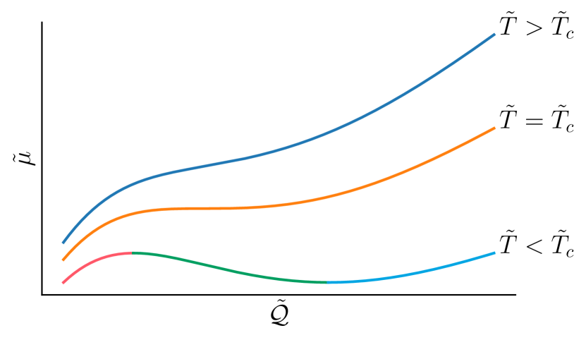
Figure 1: Plots of the equation of state (eq. (32)) for various temperatures for $\gamma^{2}=0.28$ and $J_{q}=1$. The blue and orange curves are both one-to-one functions, each corresponding to the supercritical phase at $T\geq T_{c}$. The three colors in the bottom curve correspond to $3$ different phases. Pink for the low density gaseous phase, green for the unstable phase, and blue for the high density liquid phase.

III.3 Grand potential

The grand potential is given by $\Omega=E-\mu\mathcal{Q}-T\mathcal{S}$ where ${\cal S}$ is the entropy density. Here we already have all the required relations except the entropy density.

The total energy $E=q^{2}\langle{\cal H}\rangle$ can be calculated via the effective action by considering functional derivatives. This process yields integrals over the self-energy, which we evaluate in appendix B to yield the expression in eq. (108) which we reproduce here for convenience

$$q\beta E=-\frac{4K^{2}}{U}\coth^{-1}\left[\sqrt{2\frac{K^{2}}{U^{2}}+1}\right]-2U\sqrt{2\frac{K^{2}}{U^{2}}+1}.$$ (33)

Motivated by the energy contributions, we consider an ansatz for ${\cal S}$ where the leading order is the free entropy of the system (without any interaction) and seek the leading order in $1/q$ correction. To find the leading order correction to the free entropy contribution, we use the Maxwell’s relation

$$-\left(\frac{{\partial}{\cal S}}{{\partial}{\cal Q}}\right)_{T,J_{q},J_{q/2}}=\left(\frac{{\partial}\mu}{{\partial}T}\right)_{{\cal Q},J_{q},J_{q/2}}$$ (34)

where we already know $\mu$ using the equation of state. We find that the ${\cal O}(1/q)$ contribution of entropy density is at the same order of $q$ as the energy term and the explicit expression for entropy density is given by

$${\cal S}=\ln 2-2\tilde{Q}^{2}/q+{\cal O}(q^{-2})$$ (35)

We proceed to calculate the dimensionless contribution $q\beta\Omega$ which is of order ${\cal O}(q^{0})$. We label this as $q\beta{\tilde{\Omega}}$ where we subtract off the logarithmic contribution to the entropy, namely $\tilde{\beta}{\tilde{\Omega}}=q\beta\Omega+q\ln 2$, thereby leaving us with (recall $\tilde{{\cal Q}}\equiv\sqrt{q}{\cal Q}={\cal O}(q^{0})$ in eq. (19))

$$q\beta{\tilde{\Omega}}=q\beta E-q\beta\mu{\cal Q}+2\tilde{{\cal Q}}^{2}$$ (36)

Next we use the equation of state at low-temperature given in eq. (28) combined with the scaling for $\beta$ and $\mu$ in eqs. (20) and (21), respectively. The resulting expression for $q\beta\mu{\cal Q}$ is of the order ${\cal O}(q^{0})$ and is given by

$$q\beta\mu{\cal Q}=4{\tilde{\mathcal{Q}}}^{2}[1+U\sqrt{1+2(K/U)^{2}}]$$ (37)

We already have the expression for $q\beta E$ in eq. (33) (or eq. (108) as derived in appendix B) where we see that $q\beta E\sim{\cal O}(q^{0})$. Therefore, plugging the equation of state and the energy contributions, we get

$$\tilde{\beta}{\tilde{\Omega}}=-2(1+2{\tilde{\mathcal{Q}}}^{2})U\sqrt{1+2(K/U)^{2}}-\frac{4K^{2}}{U}\coth^{-1}\left[\sqrt{[2(K/U)^{2}+1]}\right]-2\tilde{{\cal Q}}^{2}$$ (38)

where $q\beta{\tilde{\Omega}}\sim{\cal O}(q^{0})$.

Next we wish to the explicit dependence of ${\tilde{\Omega}}$ on ${\tilde{\mathcal{Q}}}$ and ${\tilde{T}}$. We use eq. (29) and recall from eq. (31) that $\gamma\equiv J_{q/2}/J_{q}$ to get as the explicit expression for the grand potential

$$\tilde{\Omega}/J_{q}=-2(1+2\tilde{\mathcal{Q}}^{2})e^{-\tilde{\mathcal{Q}}^{2}}\sqrt{1+2\gamma^{2}e^{\tilde{\mathcal{Q}}^{2}}}-4\gamma^{2}\coth^{-1}\left[\sqrt{2\gamma^{2}e^{\tilde{\mathcal{Q}}^{2}}+1}\right]-2\tilde{\mathcal{Q}}^{2}\tilde{T}/J_{q}$$ (39)

where in the limit $\gamma\rightarrow 0$, we recover the grand potential for single large-$q$ complex SYK model (eq. (6) of [4]) as it should.

IV Phase diagram

Having obtained the grand potential at low temperature, we are in a position to study the phase transition as depicted in Fig. 1. There exists a critical temperature ${\tilde{T}_{c}}$ that corresponds to the point of inflection, or in other words, when both the first derivative and the second derivative of ${\tilde{\mu}}$ with respect to ${\tilde{\mathcal{Q}}}$ vanish.

To find ${\tilde{T}_{c}}$, we start with finding the critical charge density ${\tilde{\mathcal{Q}}_{c}}$ which is obtained by imposing that the second derivative of ${\tilde{\mu}}$, given in eq. (32), with respect to ${\cal Q}$ vanish, namely ${\tilde{\mu}}^{(2)}({\tilde{\mathcal{Q}}_{c}})=0$. This equation is satisfied trivially for ${\tilde{\mathcal{Q}}_{c}}=0$ or when

$$2\gamma^{4}e^{2{\tilde{\mathcal{Q}}_{c}}^{2}}\left({\tilde{\mathcal{Q}}_{c}}^{2}-3\right)+3\gamma^{2}e^{{\tilde{\mathcal{Q}}_{c}}^{2}}\left(2{\tilde{\mathcal{Q}}_{c}}^{2}-3\right)+2{\tilde{\mathcal{Q}}_{c}}^{2}-3=0$$ (40)

Since we cannot find a simple closed form solution for ${\tilde{\mathcal{Q}}_{c}}$, we solve for $\gamma$ as a function of ${\tilde{\mathcal{Q}}_{c}}$. The positive solution is given by

$$\gamma^{2}({\tilde{\mathcal{Q}}_{c}})=e^{-{\tilde{\mathcal{Q}}_{c}}^{2}}\frac{-6{\tilde{\mathcal{Q}}_{c}}^{2}+9-\sqrt{20{\tilde{\mathcal{Q}}_{c}}^{4}-36{\tilde{\mathcal{Q}}_{c}}^{2}+9}}{4\left({\tilde{\mathcal{Q}}_{c}}^{2}-3\right)}$$ (41)

We note that $\gamma^{2}({\tilde{\mathcal{Q}}_{c}})\in[0,\infty)$ and therefore

$${\tilde{\mathcal{Q}}_{c}}\in\left[\sqrt{\frac{3}{2}},\sqrt{3}\right].$$ (42)

Indeed for the case of $\gamma^{2}({\tilde{\mathcal{Q}}_{c}})=0$, we get ${\tilde{\mathcal{Q}}_{c}}=\sqrt{3/2}$ which matches with the case of single large-$q$ complex SYK model [4] as expected.

The critical temperature is found by solving $\frac{\partial{\tilde{\mu}}}{\partial{\tilde{\mathcal{Q}}_{c}}}=0$, which yields

$$\frac{{\tilde{T}}_{c}}{J_{q}}=e^{-{\tilde{\mathcal{Q}}_{c}}^{2}}\frac{2{\tilde{\mathcal{Q}}_{c}}^{2}-1+2e^{{\tilde{\mathcal{Q}}_{c}}^{2}}\gamma^{2}({\tilde{\mathcal{Q}}_{c}})({\tilde{\mathcal{Q}}_{c}}^{2}-1)}{\sqrt{1+2e^{{\tilde{\mathcal{Q}}_{c}}^{2}}\gamma^{2}({\tilde{\mathcal{Q}}_{c}}^{2})}}$$ (43)

With this, we can now plot the parts of the EOS and grand potential corresponding to the various phases, as given in Fig. 2.

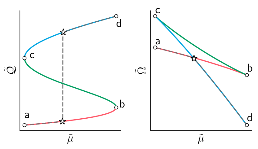
Figure 2: Plots of the equation of state (eq. (32)) and grand potential (eq. (39)) for $\gamma^{2}=0.28$, at temperature $T=0.6T_{c}$, and $J_{q}=1$.

IV.1 Universality Class

Finally, we go near the critical point on the phase diagram and expand both the chemical potential (eq. (32)) and grand potential (eq. (39)) around the critical point, including ${\tilde{\mu}_{c}}\equiv{\tilde{\mu}}({\tilde{\mathcal{Q}}_{c}})|_{T=T_{c}}$, to get the critical exponents. To do so, we first define the reduced shifted set of variables as follows:

$$m\equiv\frac{1}{a_{c}}\left[\frac{{\tilde{\mu}}}{{\tilde{\mu}_{c}}}-1\right],\;\,\rho\equiv\frac{{\tilde{\mathcal{Q}}}}{{\tilde{\mathcal{Q}}_{c}}}-1,\;\,{\tilde{T}}\equiv{\tilde{T}_{c}}\left[1+\frac{t}{b_{c}}\right]$$ (44)

such that the critical point corresponds to $m=\rho=t=0$. We have further defined

$$a_{c} \equiv\frac{1+4{\tilde{\mathcal{Q}}_{c}}^{2}(3-5{\tilde{\mathcal{Q}}_{c}}^{2}/3)+3(2{\tilde{\mathcal{Q}}_{c}}^{2}-3)\sqrt{(2{\tilde{\mathcal{Q}}_{c}}^{2}/3-1)(10{\tilde{\mathcal{Q}}_{c}}^{2}/3-1)}}{4}$$ (45)

$$b_{c} \equiv\frac{1-4{\tilde{\mathcal{Q}}_{c}}^{2}+24(2{\tilde{\mathcal{Q}}_{c}}^{2}/3)^{2}-\sqrt{(2{\tilde{\mathcal{Q}}_{c}}^{2}/3-1)(10{\tilde{\mathcal{Q}}_{c}}^{2}/3-1)}}{16(2{\tilde{\mathcal{Q}}_{c}}^{2}/3)^{2}a({\tilde{\mathcal{Q}}_{c}})}.$$

We have also rescaled the reduced shifted variables such that the overlap with the solved case of single SYK model becomes more apparent. This is the origin of the constants $a({\tilde{\mathcal{Q}}_{c}}),b({\tilde{\mathcal{Q}}_{c}})$. Such a rescaling and shifting also enters into the grand potential

$$f\equiv\frac{\tilde{\Omega}-\tilde{\Omega}_{c}}{{\tilde{\mu}_{c}}{\tilde{\mathcal{Q}}_{c}}a_{c}}+m-t/3$$ (46)

We will focus on the expansion around the critical order parameter ($\rho=0$). Using the explicit expressions in eq. (39) for the grand potential and eq. (32) for the equation of state, we expand the reduced grand potential $f$ as well as the reduced equation of state $m$ to yield

$$f =-\rho^{2}\frac{t+(3\rho/2)^{2}}{3}+{\cal O}(\rho^{5})$$ (47a)

$$m =2t/3+\rho(2t/3+\rho^{2})+{\cal O}(\rho^{4})$$ (47b)

respectively. At this point, we note that we are left with the same equations as single large-$q$ complex SYK model [4]. As such, we also have to consider field mixing to give the correct scaling function and critical exponents [21]. By this we mean that the correct ordering field $\mathscr{h}$ is not the chemical potential, but rather also gains a contribution from the temperature field, namely $\mathscr{h}\equiv m-2t/3$. We would like to express the reduced grand potential $f$ and reduced charge density $\rho$ in terms of $t$ and $\mathscr{h}$. To do this, we solve for $\rho$ in the cubic equation (47b) in terms of $t$ and $m$, use the definition of $\mathscr{h}$, then substitute in eq. (47a) and expand in various limits of either small $t$ or small $\mathscr{h}$. Since the scaling near the critical point for the reduced grand potential is found to be the same as single large-$q$ complex SYK model, the details of this procedure are already carried out in appendix C of [4]. For instance, around $\mathscr{h}=0$ for small values of $\mathscr{h}$ we get

$$f(t,\mathscr{h}) =-\frac{|t|^{2}}{6}-|\mathscr{h}||2t/3|^{1/2}-\frac{3\mathscr{h}^{2}}{2}|t|^{-1}+\mathcal{O}\left(\mathscr{h}^{3}|t|^{-5/2}\right)$$ (48)

$$\rho(t,\mathscr{h}) =\operatorname{sgn}(\mathscr{h})|2t/3|^{1/2}+2\mathscr{h}|2t/3|^{-1}+\mathcal{O}\left(\mathscr{h}^{2}t^{-5/2}\right)$$

respectively. Note that we are considering $\mathscr{h}$ to be small, but not necessarily $t$ to be small such that the term inside the big-${\cal O}$ notation is small. For small $t$ around $t=0$ (but not necessarily small $\mathscr{h}$), we also have

$$f(t,\mathscr{h}) =-\frac{3}{4}|\mathscr{h}|^{4/3}\left[1+\mathcal{O}\left(t\mathscr{h}^{-2/3}\right)\right]$$ (49)

$$\rho(t,\mathscr{h}) =-\partial_{\mathscr{h}}f(t,\mathscr{h})$$

where $f(t,\mathscr{h})$ used in the derivative is the one that has been expanded for small $t$ in eq. (49). Then we have the critical exponents $\upalpha$ calculated through specific heat $C_{\mathscr{h}}\propto-\partial_{t}^{2}f(t,0)\propto|t|^{-\upalpha}$ (using $f$ in eq. (48)), $\upbeta$ through order parameter $\rho(t,0)\propto|t|^{\upbeta}$ (using $\rho$ in eq. (48)), $\upgamma$ through susceptibility $\left.\chi_{\mathscr{h}}\propto\partial_{\mathscr{h}}^{2}f(t,\mathscr{h})\right|_{\mathscr{h}=0}\propto|t|^{-\upgamma}$ (using $f$ in eq. (48)) and $\delta$ through $\rho(0,\mathscr{h})\propto\mathscr{h}^{1/\delta}$ (using $\rho$ in eq. (49)). The critical exponents are given in table 1. These are mean-field critical exponents, and therefore our model belongs to the same universality class as van der Waals.

Table 1: Critical exponents

$\upalpha$	$\upbeta$	$\upgamma$	$\delta$
0	$\frac{1}{2}$	1	3

Surprisingly, even though the expressions for the equation of state (eq. (32)) and the grand potential (eq. (39)) are different from the case of single large-$q$ complex SYK model due to the presence of another length scale $\gamma$, we get the identical scaling of both of them around the critical point as in the case of single large-$q$ SYK model. In other words, all the above critical point expansions of the reduced equation of state $m$, the reduced charge density or equivalently the order parameter $\rho$ and the reduced grand potential $f$ are the same as that for single large-$q$ complex SYK model. Therefore, our system of coupled large-$q$ SYK models belong to the same (Landau-Ginzburg mean-field) universality class as that of a single large-$q$ complex SYK model, which in turn belongs to the van der Waals (mean-field) universality class.

V Dynamics and chaos

In this section, we will compute the Lyapunov exponent for our coupled system of complex large-$q$ SYK models and show that the model saturates the Maldacena-Shenker-Stanford (MSS) bound at low-temperature [22], thereby being maximally chaotic to order $\order{1/q}$ in the low-temperature limit.

V.1 4-point function

To obtain the Lyapunov exponent, we first analyze the four point function for the coupled system. In the large-$N$ limit, the correlator for the complex fermions $c$ is given by [1, 23]

$$\frac{1}{N^{2}}\sum_{j,k}^{N}\langle T c_{j}(\tau_{1})c_{j}^{\dagger}(\tau_{2})c_{k}^{\dagger}(\tau_{3})c_{k}(\tau_{4})\rangle=$$ (50)

$${\cal G}(\tau_{12}){\cal G}(\tau_{34})+\frac{1}{N}\mathcal{F}(\tau_{1},\tau_{2},\tau_{3},\tau_{4})+\dots$$

where the indices $j,k$ are the fermionic sites, and $\mathcal{F}=\sum_{n}\mathcal{F}_{n}$ is the unregularized out-of-time-order correlator (OTOC). The first term is a disconnected diagram, and we are interested in the $\order{\frac{1}{N}}$ diagrams. Here, the disorder average is non-vanishing if the number of indices for the two couplings $X_{\mu_{1}\dots\mu_{\kappa q/2}}^{\nu_{1}\dots\nu_{\kappa q/2}}$ (where $\kappa=\{\frac{1}{2},1\}$) are the same. As a result, the average over the product of the $q$ interaction coupling with the $q/2$ interaction is always zero. As an example, take $q=4$, for which we have the disorder average $\expectationvalue{X_{\mu_{1}\mu_{2}}^{\nu_{1}\nu_{2}}\;X_{\mu_{1}}^{\nu_{1}}}=0$.

Unlike the single large-$q$ complex SYK model, where any particular $\mathcal{F}_{n}$ in the sum denotes a single diagram [23], in our model each $\mathcal{F}_{n}$ represents a sum of ladder diagrams as depicted in Fig. (3). This is after resumming the perturbative terms to get the ladder diagrams in terms of the dressed propagators [24].

Figure 3: The diagrams related to the $\order{\frac{1}{N}}$ part of the correlator for our system of coupled complex large-$q$ SYK models. The diagram is drawn for $q=8$, and also consists of a diagram with $\tau_{3}\leftrightarrow\tau_{4}$, which have been omitted here. There are $q-2$ lines connecting the two horizontal rails, out of which Half of them ($q/2-1$ lines) run in one direction while the remaining half ($q/2-1$ lines) run in the opposite.

According to standard techniques [2, 23, 1], each diagram $\mathcal{F}_{n+1}$ is generated by applying a kernel $K$ to the previous diagram $\mathcal{F}_{n}$, i.e.,

$$\mathcal{F}_{n+1}(\tau_{1},\tau_{2},\tau_{3},\tau_{4})=\int d\tau d\tau^{\prime}K(\tau_{1},\tau_{2},\tau,\tau^{\prime})\mathcal{F}_{n}(\tau,\tau^{\prime},\tau_{3},\tau_{4})$$ (51)

or $\mathcal{F}_{n+1}=K\odot\mathcal{F}_{n}$ in short. We can recursively repeat the process and assume asymptotic exponential growth of the OTOC. The zero rung diagrams are also negligible at large times, which gives an eigenvalue problem of type $\mathcal{F}=K\odot F$ (see below for more details). The kernel for the coupled system at equilibrium is given by

$$K(\tau_{1},\tau_{2};\tau,\tau^{\prime})\equiv-\sum_{\kappa=\{\frac{1}{2},1\}}\frac{2^{\kappa q-1}J_{\kappa q}^{2}}{\kappa q}(\kappa q-1)\;{\cal G}(\tau_{1}-\tau){\cal G}(\tau_{2}-\tau^{\prime}){\cal G}^{>}(\tau-\tau^{\prime})^{\kappa q/2-1}{\cal G}^{<}(\tau^{\prime}-\tau)^{\kappa q/2-1}$$ (52)

and the generation of the ladder diagrams with the kernel is illustrated in Fig. (4). A notable result is that our kernel does not merely add a rung to the ladder diagram. It adds a sum of diagrams, where each diagram is extended with one rung.

Figure 4: In the large-$N$ limit, the diagrams of order $\order{\frac{1}{N}}$ in the out-of-time-correlator (OTOC) for the coupled SYK system can be constructed with a kernel $K$. The OTOC is then written as $\mathcal{F}=\mathcal{F}_{0}+K\mathcal{F}$, where $\mathcal{F}=\sum\limits_{n=0}^{\infty}\mathcal{F}_{n}$, where $\mathcal{F}_{0}$ is defined in Fig. 3 and becomes suppressed at large time due to exponential growth of the OTOC. This figure shows the process $\mathcal{F}_{1}=K\mathcal{F}_{0}$ for $q=8$, where the term in parentheses is the kernel.

V.2 Chaos regime

We wish to obtain the exponential growth rate of the OTOC at late times. For this, we utilize the standard approach [2, 22] by considering the following regularized out-of-time-order correlator (OTOC) in real time as

$$\mathcal{F}(t_{1},t_{2},t_{3},t_{4})=\Tr\left[y\;c_{j}(t_{1})\,y\,c_{k}^{\dagger}(t_{3})\,y\,c_{j}^{\dagger}(t_{2})\,y\,c_{k}(t_{4})\right],$$ (53)

having defined $y\equiv\rho(\beta)^{1/4}$, where $\rho(\beta)$ is the thermal density matrix. In this approach, the fermions are separated by a quarter of the thermal circle, and a real-time separation between the pairs of fermions. More on the specifics of this approach can be found in appendix C. We notice that the kernel generates all the infinite diagrams, with the exception of the free propagator, i.e.,

$$\sum\limits_{n=1}^{\infty}\mathcal{F}_{n}=K\odot\sum\limits_{n=0}^{\infty}\mathcal{F}_{n}.$$ (54)

Adding $\mathcal{F}_{0}$ on both sides and assuming asymptotic exponential growth rate of OTOC, the zero rung diagram $\mathcal{F}_{0}$ gets suppressed in the limit $t_{1},t_{2}\to\infty$. We get an eigenvalue equation of the type [23, 1] $\mathcal{F}=K\odot\mathcal{F}$, namely

$$\mathcal{F}(t_{1},t_{2},t_{3},t_{4})=\int_{\mbox{\scriptsize$-\infty$}}^{\mbox{\scriptsize$\infty$}}\!\!\!\mbox{\small$\,\mathrm{d}t$\! }\int_{\mbox{\scriptsize$-\infty$}}^{\mbox{\scriptsize$\infty$}}\!\!\!\mbox{\small$\,\mathrm{d}t^{\prime}$\! }K_{R}(t_{1},t_{2};t,t^{\prime})\mathcal{F}(t,t^{\prime},t_{3},t_{4}).$$ (55)

The exponential growth of the OTOC is determined by the real-time part of $\mathcal{F}$ , and the diagrams describing the OTOC are generated by the retarded kernel. Given the time translational invariance for our equilibrium setup, we have (with the notation from section II, namely $t_{ij}\equiv t_{i}-t_{j}$)

$$K_{R}(t_{1},t_{2};t_{3},t_{4})=\sum_{\kappa=\{\frac{1}{2},1\}}\frac{2^{\kappa q-1}J_{\kappa q}^{2}}{\kappa q}(\kappa q-1){\cal G}_{R}(t_{13}){\cal G}_{R}(-t_{24}){\cal G}_{lr}^{>}(t_{34})^{\kappa q/2-1}{\cal G}_{lr}^{<}(-t_{34})^{\kappa q/2-1},$$ (56)

where ${\cal G}_{R}$ and ${\cal G}_{lr}$ are the retarded propagator and the Wightman correlator respectively, defined as

$${\cal G}_{R}(t) \equiv[{\cal G}^{>}(t)-{\cal G}^{<}(t)]\;\theta(t)\stackrel{{\scriptstyle q\rightarrow\infty}}{{=}}\theta(t),$$ (57)

$${\cal G}^{>}_{lr}(t) \equiv{\cal G}^{>}(\imath t+\beta/2),$$

$${\cal G}^{<}_{lr}(t) \equiv{\cal G}^{<}(\imath t-\beta/2).$$

Note the relation in frequency domain between the Matsubara Green’s function and real time retarded Green’s function, namely ${\cal G}({\imath}\omega_{n}\to\omega+{\imath}0^{+})={\cal G}_{R}(\omega)$ [25]. Compared with the kernel in eq. (52), we see that the overall minus sign vanishes. This is due to the transformation $\tau\to it$ and $\tau^{\prime}\to it^{\prime}$, leading to $d\tau d\tau^{\prime}=-dtdt^{\prime}$ in the integral of type of eq. (55), where the minus sign is absorbed in the retarded kernel. For a detailed discussion on the retarded kernel and the chaos exponents in real time, see [26] (in particular, section 8).

The explicit form of the Wightman function can be found with the Green’s function in eqs. (5) and (12). Combined with the effective coupling (8), we have (recall $\cosh(-t)=\cosh(t)$)

$$K_{R}(t_{1},t_{2};t_{3},t_{4})=\theta(t_{13})\theta(t_{24})B(t_{34}),$$ (58)

where

$$B(t_{34})\equiv\frac{2(\pi v)^{2}A^{2}\;\theta(t_{13})\theta(t_{24})}{\beta^{2}\left[1+\sqrt{A^{2}+1}\cosh(\frac{\pi vt_{34}}{\beta})\right]^{2}}+\frac{(\pi v)^{2}\;\theta(t_{13})\theta(t_{24})}{\beta^{2}\left[1+\sqrt{A^{2}+1}\cosh(\frac{\pi vt_{34}}{\beta})\right]}.$$ (59)

Recall the definition of $A$ from eq. (13), namely $A\equiv\frac{\pi v\beta\mathcal{J}_{q}}{\left(\beta\mathcal{J}_{q/2}\right)^{2}}$ $=\frac{\pi vU}{qK^{2}}$ where we used definitions in eq. (22) and the scaling for $\beta$ in eq. (20). It is important to notice that even if the kernel applies multiple diagrams, the total sum of infinite diagrams in $\mathcal{F}$ does not change with applying the retarded kernel. Furthermore, the zero rung ladder diagram gets suppressed at larger times. This implies that in the coupled SYK model, $\mathcal{F}$ is also an eigenfunction of the integral transform that can be further simplified by taking the two derivatives $\partial_{t_{1}}\partial_{t_{2}}$ on both sides of the integral equation (eq. (55)) to get

$$\partial_{t_{1}}\partial_{t_{2}}\mathcal{F}(t_{1},t_{2},t_{3},t_{4})=\int_{-\infty}^{\infty}dt\int_{-\infty}^{\infty}dt^{\prime}\;\delta(t_{1}-t)\delta(t_{2}-t^{\prime})B(t_{34})\;\mathcal{F}(t,t^{\prime},t_{3},t_{4}).$$ (60)

The delta functions enforces $t=t_{1}$ and $t^{\prime}=t_{2}$. Due to the theta function and our interest in large times $t_{1}$ and $t_{2}$, we can put $t_{3}=t_{4}=0$ without loss of generality. For brevity, we write $\mathcal{F}(t_{1},t_{2},t_{3}=0,t_{4}=0)=\mathcal{F}(t_{1},t_{2})$.

V.3 The Lyapunov exponent

To solve this integral in real time, assuming a chaotic behavior at asymptotic times, we make the standard ansatz [2, 1, 23]

$$\mathcal{F}(t_{1},t_{2})=e^{\lambda_{L}(t_{1}+t_{2})/2}f(t_{12}),$$ (61)

where $\lambda_{L}$ is the growth exponent, known as the Lyapunov exponent. With the ansatz (61), and assuming the function $\mathcal{F}(t_{1},t_{2})$ decays at the boundaries $t_{1},t_{2}\to-\infty$, this reduces to a second order differential equation

$$\left[\partial_{t_{1}}\partial_{t_{2}}-B(t_{12})\right]f(t_{12})=-\frac{\lambda_{L}^{2}}{4}f(t_{12}).$$ (62)

In fact, it is a “Schrödinger equation” with a potential

$$V(x)\equiv-2B(t_{12})/(\pi vT)^{2},\qquad x\equiv\pi vTt_{12}/2.$$ (63)

From the chain rule we then have

$$\partial_{t_{1}}\partial_{t_{2}}=\frac{\partial x}{{\partial}t_{1}}\frac{\partial x}{{\partial}t_{2}}{\partial}_{x}^{2}=-\frac{(\pi vT)^{2}}{2}{\partial}_{x}^{2}/2$$

which leaves us with

$$\left[-{\partial}_{x}^{2}/2+V(x)\right]f(t_{12})=-\frac{\lambda_{L}^{2}}{2(\pi vT)^{2}}f(t_{12}).$$ (64)

While there typically exists an entire spectrum of Lyapunov exponents, the system’s chaos is defined by the maximum $\lambda_{L}$. This corresponds to the minimal negative eigenvalue, which would correspond to the ground state energy $E_{0}$. As such, we have a ground state wave function $\psi_{0}(x)\equiv f(t_{12})$ and energy

$$E_{0}\equiv-\frac{\lambda_{L}^{2}}{2[\pi vT]^{2}}.$$ (65)

This leaves us with the more familiar form of the Schrödinger equation

$$\left[-\frac{{\partial}_{x}^{2}}{2}+V(x)\right]\psi_{0}(x)=E_{0}\psi_{0}(x).$$ (66)

V.3.1 Perturbation theory

Let us now consider the above Schrödinger type equation (66) and in particular the potential, which may be written as

$$V(x)= \frac{1}{(\sqrt{A^{2}+1}-1)/2+\sqrt{A^{2}+1}\,/V_{0}(x)}$$ (67)

$$-\frac{A^{2}}{[(\sqrt{A^{2}+1}-1)/2+\sqrt{A^{2}+1}\,/V_{0}(x)]^{2}}$$

where $A\equiv\frac{\pi v\beta\mathcal{J}_{q}}{\left(\beta\mathcal{J}_{q/2}\right)^{2}}$ $=\frac{\pi vU}{qK^{2}}$. We now consider this for small $A$, with corrections $\psi_{0}=\psi_{0}^{(0)}+A^{2}\psi_{0}^{(1)}+\ldots$ and $E_{0}=E_{0}^{(0)}+A^{2}E_{0}^{(1)}+\ldots$ obtained via perturbation theory.

For $A=0$, we are left with the Pöschl-Teller potential $V_{0}(x)=-\sech^{2}(x)$ [27] and the ground state is

$$\psi_{0}^{(0)}(x)=\sech(x)/\sqrt{2}.$$ (68)

with corresponding eigenvalue is $E_{0}^{(0)}=-1/2$. The leading order perturbed potential is

$$V(x)=V_{0}(x)-\frac{V_{0}(x)}{4}(2+33V_{0}(x))A^{2}+{\cal O}(A^{4})$$ (69)

As such, first order perturbation theory yields the energy correction $E_{0}=-1/2+A^{2}E^{(1)}_{0}+{\cal O}(A^{4})$, with

$$E^{(1)}_{0}=-\bra{\psi^{(0)}_{0}}\frac{\hat{V}_{0}}{4}(2+33\hat{V}_{0})\ket{\psi^{(0)}_{0}}.$$ (70)

Inserting the identity $\int dx|x\rangle\langle x|=1$ yields

$$E^{(1)}_{0} =\int_{\mbox{\scriptsize$$}}^{\mbox{\scriptsize$$}}\!\!\!\mbox{\small$\,\mathrm{d}x$\! }\frac{V_{0}^{2}(x)}{8}(2+33V_{0}(x))$$ (71)

This integrates to $E^{(1)}_{0}=-61/15$, hence the energy is lowered. Since we have the Lyapunov exponent (65)

$$\lambda_{L}=\sqrt{2|E_{0}|}\pi vT,$$ (72)

one might assume that this leads to an increase to the exponents, hence allowing one to surpass the MSS bound. Note however that this correction is actually at quadratic order since

$$A=\frac{\pi vU}{qK^{2}}$$ (73)

whereas there is another correction to $v$ in eq. (26) which reduces the Lyapunov exponent at linear order, namely

$$v=2-\frac{4}{qK}\sqrt{2+(U/K)^{2}}+{\cal O}(q^{-2})$$ (74)

As such the MSS bound $\lambda_{L}\to 2\pi T$ remains intact in the low $T$ limit. We can now return to the topic of $v$ being twice that of the $q$-body SYK model. The point is that $v$ is not necessarily a direct measure of chaos in the usual sense of single SYK model. While $\lambda_{L}=\sqrt{2|E_{0}|}\pi vT$ remains true, if we had instead first set $\gamma=0$ (implying $A\to\infty$), we would have found a potential using eq. (67)

$$V(x)\sim-\frac{1}{[1/2+1/V_{0}(x)]^{2}}=V_{0}(2x)/4.$$ (75)

This then leads to a ground state energy of $E_{0}=2$ and $v\to 1$ in the low-temperature regime [1]. Said another way, while $v$ might saturate to either $1$ or $2$, in either of these cases, the Lyapunov exponent will saturate to the MSS bound.

V.4 Relation to the phase transitions at “very” low-temperature

Given that the MSS bound is always saturated over the phase transition corresponding to the temperature regime $T={\cal O}(q^{-1})$ (20), we conclude that both liquid and gaseous phases are maximally chaotic. In other words, we have a maximally chaotic to maximally chaotic phase transition similar to those found in small to large black hole phase transitions [3, 7].

This, however, changes in the rescaled regime of very low-temperature

$$T=\bar{T}q^{-2}={\cal O}(q^{-2}),$$ (76)

(equivalently $\bar{\beta}=\beta q^{-2}$) which is the regime one must consider to carefully take the zero temperature limit. The chemical potential scaling is defined as $\mu\equiv\bar{\mu}q^{2}$. In this regime, much like the standard $q$-body SYK model, the “gaseous” and “liquid” densities diverge [4]. The terminologies are used in accordance with the van der Waals gas as we have already seen that both belong to the same universality class. This is highlighted in Fig. 5. In fact, the liquid phase, the blue line in Fig. 1 (also see Fig. 5), is at $Q_{\ell}={\cal O}(q^{0})$ while the gaseous phase has ${\cal Q}_{g}={\cal O}(q^{-1})$. Now recall that the effective SYK interactions have a Gaussian suppression in charge density. As such, the large charge density of the liquid eventually fully suppresses the SYK interactions, leaving a free non-interacting liquid

$$\tilde{\Omega}_{\ell}=\frac{\bar{T}}{2}\ln[1-4{\cal Q}_{\ell}^{2}],\quad\bar{\mu}_{\ell}=2\bar{T}\tanh^{-1}(2{\cal Q}_{\ell}),$$ (77)

where recall that we have defined $\bar{\mu}\equiv\mu q^{-2}$.

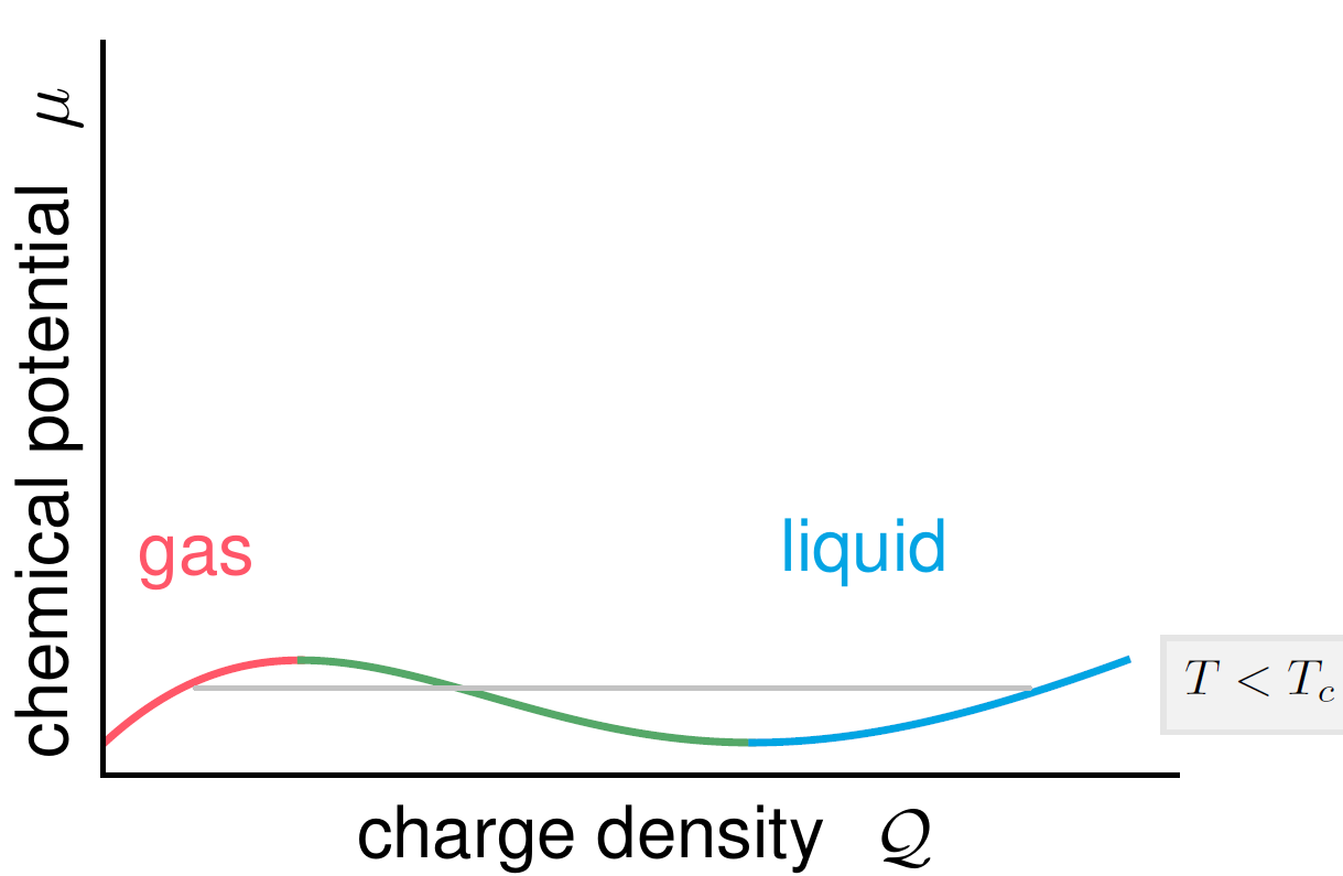
Figure 5: Liquid and gaseous phases for temperatures below the critical temperature, where we have borrowed terminology from the van der Waals phase transition that belongs to the same universality class as our coupled SYK system. Color coding is the same as in Figs. 1 and 2.

With this in mind, let us consider the mathematical details around the phase transition in this rescaled regime. The full EOS (18) may be written as

$$\bar{\beta}\bar{\mu}=\ln\left[\frac{1+2{\cal Q}}{1-2{\cal Q}}\right]-2{\cal Q}q\bar{\beta}\alpha.$$ (78)

For the case where $\gamma=0$, we know that, at such temperatures and chemical potentials, the phase transition is from ${\cal Q}$ of order ${\cal O}(1/q)\to{\cal O}(q^{0})$ [4]. Let us consider the EOS and the grand potential here for such charge densities. As for the $\gamma=0$ case, for charge densities ${\cal Q}={\cal O}(q^{0})$, the Lyapunov exponent is exponentially suppressed, $v\sim e^{-q{\cal Q}^{2}}\to 0$, hence the system is free. Here we set $J_{q}=1$, since we will not focus on the case where $J_{q}=0$.

For ${\cal Q}_{g}=\bar{{\cal Q}}_{g}q^{-1}$, we find the gaseous phase still remains in the maximally chaotic phase. This leaves us with the gaseous part of the EOS

$$\bar{\mu}_{g}\sim 4\bar{{\cal Q}}_{g}\sqrt{2\gamma^{2}+1}$$ (79)

and the grand potential (39)

$$\tilde{\Omega}_{g}=-2\sqrt{1+2\gamma^{2}}-4\gamma^{2}\coth^{-1}\sqrt{2\gamma^{2}+1}.$$ (80)

The phase transition will be where (80) and (79) are equal to (77). Equating the two expressions, we find that

$${\cal Q}_{\ell}=\frac{\sqrt{1-e^{2\bar{\beta}\tilde{\Omega}_{g}}}}{2}\xrightarrow[\bar{T}\to 0]{}1/2$$

and

$$\bar{{\cal Q}}_{g}=\bar{T}\frac{\tanh^{-1}(2{\cal Q}_{\ell})}{2\sqrt{2\gamma^{2}+1}}\xrightarrow[\bar{T}\to 0]{}-\frac{\tilde{\Omega}_{g}}{2\sqrt{1+2\gamma^{2}}}$$

So for the liquid phase, we have a relatively high density ${\cal Q}_{\ell}={\cal O}(q^{0})$. Recall that such a density leads to exponential suppression in the effective couplings (8) ${\cal J}_{\kappa q}\lesssim e^{-\kappa q{\cal Q}_{\ell}^{2}}J_{\kappa q}$. As such, despite the linear $q$ growth stemming from the smaller temperature in $K,U$, defined in eq. (22) or equivalently in eq. (29), we find using the scaling relations (20) and (76) that, in this liquid regime, both $K$ and $U$ are smaller than $q\bar{\beta}e^{-q{\cal Q}^{2}}$. The exponential suppression dominates over any polynomial growth in $q$, implying that the closure relation (24)

$$\pi v=\sqrt{\frac{U^{2}}{q^{2}}+\left(\frac{K^{2}}{\pi v}\right)^{2}}q^{2}\cos(\pi v/2)+\frac{q^{2}K^{2}}{\pi v},$$ (81)

reduces to $\pi v\sim 0$. We have plotted the phase diagram for low and “very” low temperatures in Fig. 6 for any finite value of $\gamma$. As such, we have also confirmed that the free liquid state is indeed regular (non-chaotic), with a Lyapunov exponent of $\lambda_{L}=0$. As such, we are left with a maximally chaotic to regular phase transition, which is similar to that of the standard Hawking-Page transition from a large black hole to non-interacting radiation [8] but as stated in the introduction, instead of having a particular value of temperature like in Hawking-Page, we have an entire region of temperatures in the very low-temperature regime in our coupled SYK case where we observe maximally chaotic to non-chaotic first order phase transition. We discuss this in the next subsection.

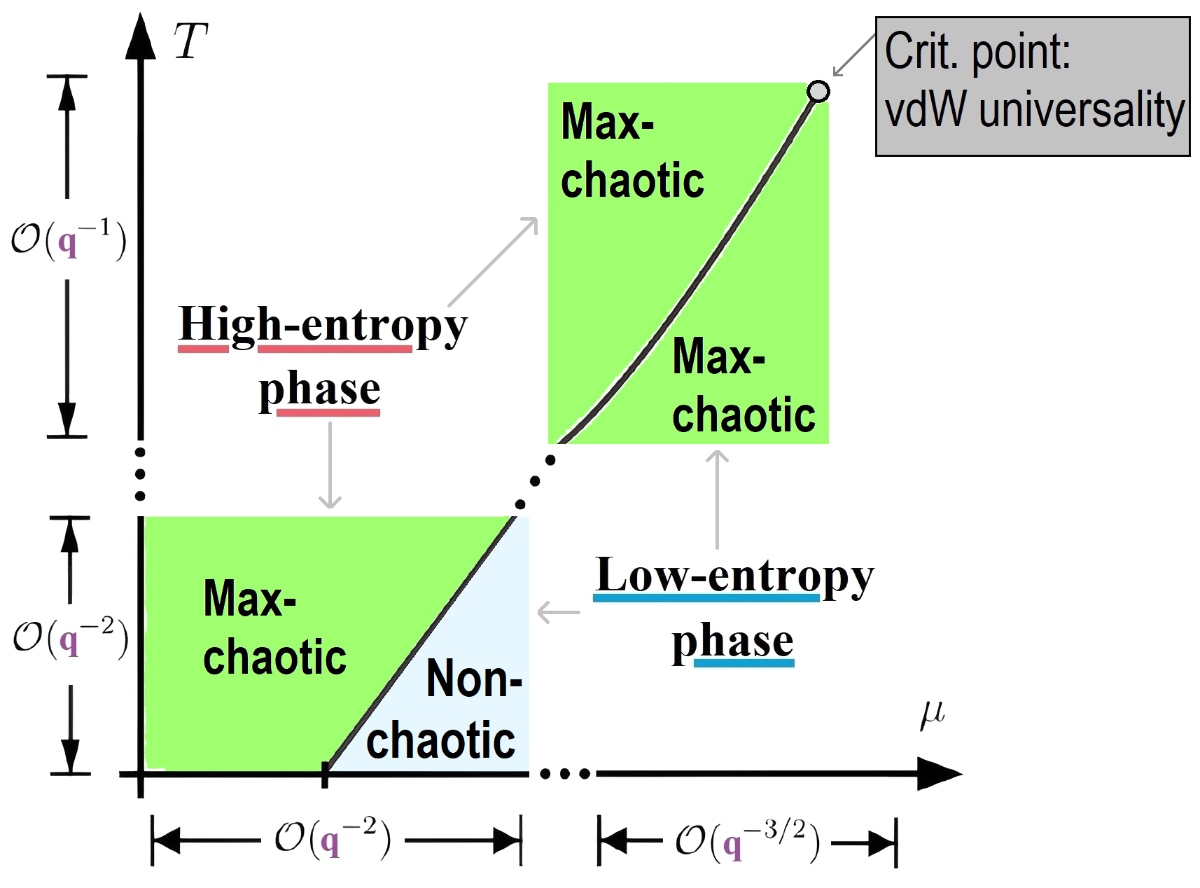
Figure 6: Phase diagram for our coupled SYK system for any finite value of $\gamma$ at low and “very” low temperatures, as discussed in section V.4.

V.5 Comparing with the Hawking-Page transition

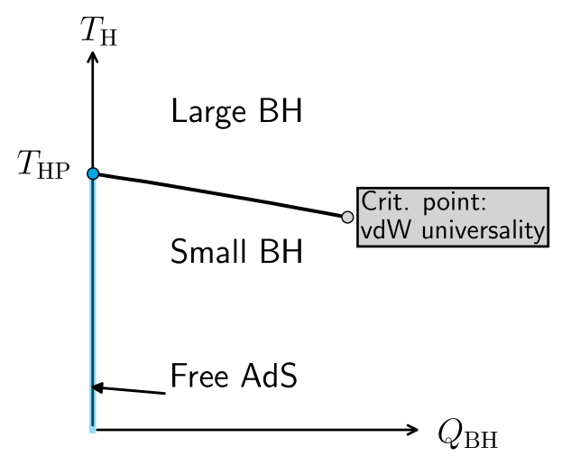
Figure 7: Phase diagram for charged ADS black hole where $T_{H}$ is the Hawking temperature, $Q_{\text{BH}}$ is the total charge of the black hole and $T_{\text{HP}}$ is the Hawking-Page temperature.

We return to the remark made in the introduction (section I) where we compare our observed phase transition (see the phase diagram in Fig. 6) with the Hawking-Page transition. Following the lead of [28, 29], we present the phase diagram of a charged AdS black hole in Fig. 7. As clear from the figure, the charge-less ($Q_{\text{BH}}=0$) case has a Hawking-Page transition where, for temperature $T<T_{\text{HP}}$, we have a free (non-chaotic) radiation while a black hole (maximally chaotic) is preferred for temperatures $T>T_{\text{HP}}$. This is a first order phase transition. For all nonzero values of $Q_{\text{BH}}\neq 0$, we have a maximally chaotic large black hole to maximally chaotic small black hole. Contrast this with Fig. 6 where for low temperatures ($T={\cal O}(q^{-1})$), we observe the same behavior as in Fig. 7 but for “very” low temperatures ($T={\cal O}(q^{-2})$), we obtain an entire regime of maximally chaotic to non-chaotic first order phase transition in contrast to Fig. 7 where this happens only along the vertical-axis where $Q_{\text{BH}}=0$. This is what we meant in the introduction and at the end of the previous subsection that for our coupled SYK system, just like single SYK model, due to the presence of this entire range of “very” low temperatures, the mapping on the black hole side to a standard Hawking-Page transition is not reproduced.

Before we end this section, we would like to comment on Fig. 7 which we reproduce from [28, 29]. The analysis was reproduced and generalized to the charged case in [7] where the authors called the temperature of transition as the “Zorro’s” temperature when $Q_{\text{BH}}=0$ on the coexistence line. As highlighted in appendix D, we show that this temperature is indeed the same as Hawking-Page temperature and the horizontal-axis of Fig. 13 in [7] (as reproduced with more details here in Fig. 7 taken from [28], [29]) is the standard Hawking-Page first order phase transition from a maximally chaotic black hole to non-chaotic free radiation (recall this is true only when $Q_{\text{BH}}=0$) as one cools the temperature down to the Hawking-Page temperature $T_{\text{HP}}$ which is referred to as the “Zorro’s” temperature in [7].

VI Conclusion and Outlook

Motivated from the study of a single large-$q$ complex SYK model, we considered a system of coupled SYK models in this work and studied its thermodynamic and dynamic properties. Despite having a new scale in the system, namely the ratio of interaction strengths of the two SYK terms in the Hamiltonian, we found that there exists a continuous phase transition at low temperatures just like the single SYK and the associated critical exponents correspond to the same universality class as Landau-Ginzburg (mean-field) exponents, also shared by van der Waals gas. Coincidentally, various AdS black holes also belong to the same universality class [7, 30]. We will comment more on this below. Finally, we calculated the Lyapunov exponent, and we again found that the coupled SYK system also saturates the Maldacena-Shenker-Stanford (MSS) bound in large-$q$ limit at low temperature, thereby making our model maximally chaotic, surprisingly matching the behavior of the single SYK model.

The coupled SYK system’s adherence to the established Landau-Ginzburg universality class and its demonstration of maximal chaos are not merely mathematical curiosities. They provide a critical lens through which the fundamental nature of quantum chaos and gravity can be examined. This universality across different models and configurations raises the question of how one can obtain deviating results. Given that we flow to the identical grand potential scaling relations near a critical point for the combination of two SYK models, the natural question to ask is to what extent this result can be generalized. Does it hold for any system of coupled large-$q$ type SYK models with the Hamiltonian given by

$${\cal H}=\sum_{\kappa>0}J_{\kappa}{\cal H}_{\kappa q}$$ (82)

or does it extend beyond this, or is it just a coincidence that we found for our coupled case? Given that the kinetic SYK model is integrable, one would imagine this to change upon adding a quadratic term to the above Hamiltonian. This term would dominate in the low-temperature regime, which would at least mean that the model is unlikely to have a maximally chaotic to maximally chaotic second order phase transition, as observed in this work. But without any kinetic term, the future work can be to find if at large-$q$ and low-temperature limits, all coupled SYK systems as in eq. (82) belong to the same universality class as Landau-Ginzburg and if they are also maximally chaotic.

Looking ahead, our study naturally leads to the exploration of holographic mappings of these coupled systems to $1+1$-dimensional gravity, analogous to what has been achieved for the single SYK model [3]. As we have found that the scaling relations near the critical point are the same as the single SYK model, essentially what we have to do is to match our grand potential of the coupled SYK system to that of the single SYK model. Then we use the dictionary developed in [3] to the deformed JT gravity to find the necessary modifications on the gravity side. We expect to find a phase transition on the gravity side between a small and a large black hole (for example, see [7]) that corresponds to the chaotic-to-chaotic continuous phase transition as obtained for our model. More importantly, the modifications to be done on the SYK side to reproduce an exact Hawking-Page type first order phase transition, as discussed in detail in section V.5, will be quite an interesting and welcoming result. We leave these for the future work.

Appendix A Derivation of differential equation for Green’s function

For our model in eq. (1), the self-energy $\Sigma$ here is just the sum of the individual self-energies, $\Sigma=\Sigma_{q}+\Sigma_{q/2}$ where $\Sigma_{\kappa q}$ ($\kappa=\{1/2,1\}$) is defined below [1]. This enters into the Dyson equation ${\cal G}^{-1}={\cal G}_{0}^{-1}-\Sigma$, where ${\cal G}_{0}$ is the free Green’s functions.

We start with the definition of effective coupling coefficients in eq. (8). This allows us to define another quantity

$${\cal L}^{>}(t_{1},t_{2})\equiv\sum_{\kappa\in\{\frac{1}{2},1\}}2{\cal J}_{\kappa}^{2}e^{\kappa g_{+}(t_{1},t_{2})},{\cal L}^{<}(t_{1},t_{2})={\cal L}^{>}(t_{1},t_{2})^{*}$$ (83)

where we reproduce the definition of the effective couplings for the Hamiltonian in eq. (1) as

$${\cal J}_{\kappa q}\equiv(1-4{\cal Q}^{2})^{\kappa q/4-1/2}J_{\kappa q}$$ (84)

This contributes to the self-energy [19] of both terms in the Hamiltonian, as

$$\Sigma_{\kappa q}^{\gtrless}(t_{1},t_{2})=\frac{1}{q}{\cal L}^{\gtrless}(t_{1},t_{2}){\cal G}^{\gtrless}(t_{1},t_{2})$$ (85)

We are interested in obtaining the differential equations for $g^{\pm}$ whose solutions will solve our model. We start with the differential equations for $g^{\gtrless}$ (plugging eq. (20) into eq. (19) in [19]) where the Kadanoff-Baym equations reduce to the following:

$$\partial_{t_{1}}g^{\gtrless}(t_{1},t_{2})=\int_{t_{1}}^{t_{2}}dt_{3}{\cal L}^{\gtrless}(t_{1},t_{3})+\underbrace{2{\cal G}^{\lessgtr}(0,0)}_{2{\cal Q}\pm 1}{\imath}\alpha(t_{1}).$$ (86)

Here $\alpha$ is related to the expectation value of energy per particle given by

$$(1-{\cal Q}^{2})\alpha(t)=\epsilon_{q/2}(t)/2+\epsilon_{q}(t)$$ (87)

where in the large-$q$ limit, we have ${\cal Q}={\cal O}(q^{-1/2})$ and $\epsilon_{\kappa q}(t)$ is defined as

$$\epsilon_{\kappa q}(t)\equiv q^{2}\frac{J_{\kappa q}\langle{\cal H}_{\kappa q}\rangle}{N}$$ (88)

where $\kappa\in\{\frac{1}{2},1\}$.

We take the differential equation for $g^{<}(t_{1},t_{2})$ and take its complex conjugate to get the differential equation for time reversed $g^{<}(t_{2},t_{1})$ given by (recall ${\cal L}^{<}(t_{1},t_{2})={\cal L}^{>}(t_{1},t_{2})^{*}$)

$${\partial}_{t_{1}}g^{<}(t_{2},t_{1})=\int_{\mbox{\scriptsize$t_{1}$}}^{\mbox{\scriptsize$t_{2}$}}\!\!\!\mbox{\small$\,\mathrm{d}t_{3}$\! }{\cal L}^{>}(t_{1},t_{3})-\left(2{\cal Q}-1\right){\imath}\alpha(t_{1})$$ (89)

We add and subtract this to the differential equation for $g^{>}(t_{1},t_{2})$ to get

$${\partial}_{t_{1}}g^{+}(t_{1},t_{2}) =\int_{t_{1}}^{t_{2}}dt_{3}{\cal L}^{>}(t_{1},t_{3})+{\imath}\alpha(t_{1})$$ (90)

$${\partial}_{t_{1}}g^{-}(t_{1},t_{2}) =2{\cal Q}{\imath}\alpha(t_{1})$$

We recall that we are only interested in the equilibrium situation, implying that all expectation values are constant, hence $\alpha(t)$ is constant as well as the Green’s functions are only dependent on time differences $g^{\pm}(t_{1},t_{2})\equiv g^{\pm}(t_{1}-t_{2})$. Therefore, we solve the above differential equation for $g^{-}$ to get

$$g^{-}(t_{1},t_{2})=2{\cal Q}{\imath}\alpha\cdot(t_{1}-t_{2})$$ (91)

and obtain a second order differential equation for $g^{+}$ given by

$${\partial}_{t_{1}}{\partial}_{t_{2}}g^{+}(t_{1}-t_{2})={\cal L}^{>}(t_{1},t_{2})$$ (92)

We finally plug the definition of ${\cal L}^{>}$ from eq. (83) above to get the differential equation for $g^{+}$ (where $t_{1}-t_{2}\equiv t$)

$$\ddot{g}^{+}(t)=-2{\cal J}_{q}^{2}e^{g_{+}(t)}-2{\cal J}_{q/2}^{2}e^{g_{+}(t)/2}$$ (93)

Thus we have solved for $g^{-}$ (eq. (91)) and obtained the differential equation for $g^{+}$ whose solution is presented in the main text in eq. (12), thereby solving the system.

Appendix B Energy contributions

The energy contributions in eq. (87) can also be derived by the integral expression for $\alpha(t)$ [17]. Asymptotically in the large-$q$ limit using eq. (5) and the scaling of ${\cal Q}$ mentioned in eq. (19), we get to leading order in $1/q$ (see eqs. (19) to (20) in [19])

$$\alpha(t_{1})={\imath}\int_{\mbox{\scriptsize$-\infty$}}^{\mbox{\scriptsize$t_{1}$}}\!\!\!\mbox{\small$\,\mathrm{d}t_{3}$\! }\left(q\Sigma^{>}(t_{1}-t_{3})-q\Sigma^{<}(t_{1}-t_{3})\right)$$ (94)

where using eq. (85), we have

$$q\Sigma_{\kappa q}^{>}(t_{1},t_{2})\sim-{\cal L}^{>}(t_{1},t_{2})/2$$ (95)

and ${\cal L}^{<}(t_{1},t_{2})={\cal L}^{>}(t_{1},t_{2})^{*}$, leaving

$$\alpha(0)={\operatorname{Im}}\int_{\mbox{\scriptsize$-\infty$}}^{\mbox{\scriptsize$0$}}\!\!\!\mbox{\small$\,\mathrm{d}t$\! }{\cal L}^{>}(-t)$$ (96)

Note from eq. (87) that ${\cal Q}^{2}\sim{\cal O}(1/q)$ and therefore to leading order in $1/q$, we have $\alpha$ equal to the weighted energy sum (which is also a constant as we are considering equilibrium situation) given by

$$\alpha(0)=\sum_{\kappa=\frac{1}{2},1}\kappa\epsilon_{\kappa q}(0)$$ (97)

Therefore, we can isolate the individual energy integrals as

$$\kappa\epsilon_{\kappa q}(0)={\operatorname{Im}}\int_{\mbox{\scriptsize$-\infty$}}^{\mbox{\scriptsize$0$}}\!\!\!\mbox{\small$\,\mathrm{d}t$\! }2{\cal J}^{2}_{\kappa q}e^{\kappa g^{+}(-t)}$$ (98)

We first evaluate $\epsilon_{q/2}$ where we substitute eq. (12) for $e^{g^{+}(-t)}$ to get

$$\beta\epsilon_{q/2}(t_{1}) ={\operatorname{Im}}\int_{\mbox{\scriptsize$-\infty$}}^{\mbox{\scriptsize$0$}}\!\!\!\mbox{\small$\,\mathrm{d}t$\! }4\beta^{2}T{\cal J}_{q/2}^{2}e^{g^{+}(-t)/2}$$ (99)

$$={\operatorname{Im}}\int_{\mbox{\scriptsize$-\infty$}}^{\mbox{\scriptsize$0$}}\!\!\!\mbox{\small$\,\mathrm{d}x$\! }\frac{4\pi v}{1+B\cos(\pi v/2+{\imath}x))}$$

where we have let $x=\pi vTt$ and $B=\sqrt{A^{2}+1}$. Recall that $A$ is given by eq. (23)

$$A=\frac{\pi vU}{qK^{2}}.$$ (100)

The integral is solved to get

$$-\frac{8{\imath}\pi v}{A}\tanh^{-1}\left[\left(\sqrt{A^{-2}+1}-A^{-1}\right)\tan(\pi v/4+{\imath}x/2)\right]$$ (101)

where $x\rightarrow-\infty$ is a purely real contribution thereby dropping out (since we are interested in the imaginary part of the integral only) and at $x=0$, we are left with

$$-\frac{8{\imath}\pi v}{A}\tanh^{-1}\left[\left(\sqrt{A^{-2}+1}-A^{-1}\right)\tan(\pi v/4)\right]$$ (102)

Therefore we have the final expression as

$$\beta\epsilon_{q/2}(t_{1})=-\frac{8\pi v}{A}\tanh^{-1}\left[\left(\sqrt{A^{-2}+1}-A^{-1}\right)\tan(\pi v/4)\right]$$ (103)

In the limiting case of ${\cal J}_{q}\rightarrow 0$, we are left with $A\rightarrow 0$, thereby leading to

$$\beta\epsilon_{q/2}(t_{1})=-4\pi v\tan(\pi v/4)$$ (104)

which is the correct energy density for single large-$q/2$ complex SYK model. Furthermore, considering the (scaled) low-temperature case

$$T={\tilde{T}}/q={\cal O}(q^{-1}),\quad\beta=q\tilde{\beta},$$ (105)

we find $A={\cal O}(q^{-1})$ implying that the obtained result is still the correct leading order result.

Next we proceed to calculate $\epsilon_{q}$. We know that to the leading order in $1/q$, we have $\alpha=\epsilon_{q}+\frac{1}{2}\epsilon_{q/2}$. Here we already know $\alpha$ from eq. (27) which is at low-temperature and $\epsilon_{q/2}$ from eq. (103). Therefore we get

$$E =\langle{\cal H}/N\rangle=\epsilon_{q/2}/q^{2}+\epsilon_{q}/q^{2}$$ (106)

$$=\epsilon_{q/2}/q^{2}+(\alpha-\epsilon_{q/2}/2)/q^{2}$$

which can be re-arranged as follows:

$$q\beta E=\beta\epsilon_{q/2}/(2q)+\beta\alpha/q$$ (107)

where using the scaling for $\beta$ in eq. (105), we immediately see that $\alpha$ and $q\beta E$ are both at order ${\cal O}(q^{0})$. Then we substitute eqs. (27) and (103) to finally get the full expression for the energy in the (scaled) low-temperature limit as

$$q\beta E=-\frac{4K^{2}}{U}\coth^{-1}\left[\sqrt{2\frac{K^{2}}{U^{2}}+1}\right]-2U\sqrt{2\frac{K^{2}}{U^{2}}+1}$$ (108)

Appendix C Chaos theory of the SYK model

In chaos theory, we wish to analyze the evolution of the systems operator $W(t)$ after a small perturbation $V(0)$ in the initial conditions. The correlation function describing this evolution is the out-of-time-order correlator (OTOC), generally written as

$$c(t)=\expectationvalue{[W(t),V(0)]^{2}}_{\beta},$$ (109)

where $\expectationvalue{\dots}_{\beta}$ is the thermal expectation value, which can be written as $\expectationvalue{{\cal O}}_{\beta}=\Tr[\rho(\beta){\cal O}]=\frac{1}{Z}\Tr[e^{\beta H}{\cal O}]$. It has been noticed that the correlator grows exponentially with some growth rate $\lambda_{L}$ [2],

$$c(t)\sim e^{\lambda_{L}t},$$ (110)

and the goal is to find this grow rate. The exponential growth of the OTOC depends on real time, and thus we wish to compute the correlator in real time.

A common and convenient choice of writing the OTOC in SYK models is [22]

$$\mathcal{F}(t_{1},t_{2})=\Tr\left[y\;W(t)\;y\;V(0)\;y\;W(t)\;y\;V(0)\right],\quad y\equiv\rho(\beta)^{1/4}$$ (111)

where $\rho(\beta)$ is the thermal density matrix. This choice is to make computation easier, and will not affect the exponent [22, 31]. For simplicity, we have illustrated the OTOC with a Keldysh-Schwinger contour in figure (8).

Figure 8: On the left is the Keldysh-Schwinger contour for the out-of-time-correlator (OTOC) for the chaotic system. The perturbation $V(0)$ and generic operator $W(t)$ are separated by a large real time and a quarter on the thermal circle, as is shown in the picture on the right.

Here, the operators are separated by a quarter on the thermal circle (for details, see [1]), and additionally a real-time separation between the pair of operators. We are interested in regimes where $t\rightarrow\infty$, such that the zero rung diagrams, can be neglected. The paths in real time are described by the retarded propagator defined as (57), and the Wightman Greens function (57) describes a pair of operators separated by $\beta/2$ on the thermal circle. If we evaluate the Greens function (12) with $t\rightarrow it+\beta/2$, we see that the function becomes a function of real time. Hence, this operation can be seen as an analytic continuation to real time.

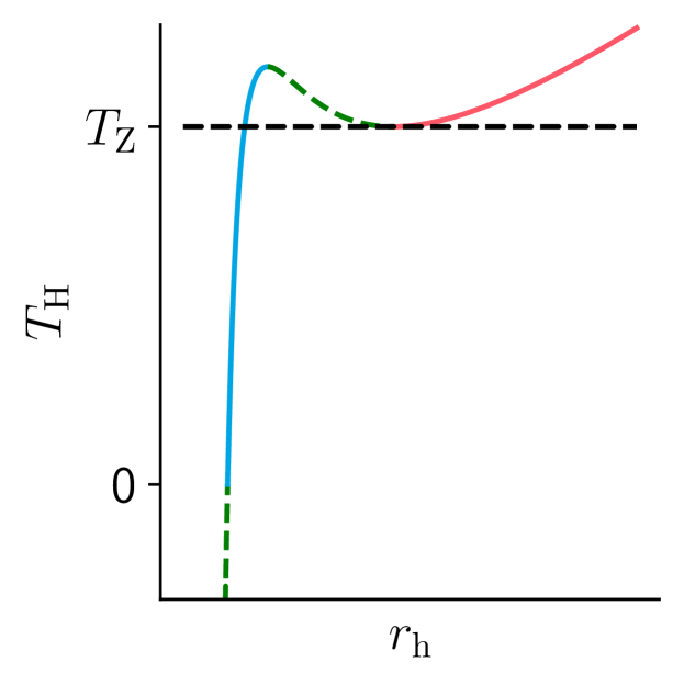
Figure 9: Equation of state for charged ADS black hole where $T_{H}$ is the Hawking temperature, $Q_{\text{BH}}>0$ is the total charge of the black hole and $T_{\text{Z}}$ is the minimum temperature of the larger black hole. The green dashed lines are the unstable regimes with negative specific heat. The two stable phases are marked with blue and red. Color coding is the same as in Figs. 1, 2 and 5.

Appendix D “Zorro’s” temperature and the Hawking-Page transition

For a Reissner–Nordström black hole, we find the Hawking temperature

$$T_{\text{H}}=\frac{1}{4\pi r_{\text{H}}}\left(1+8\pi r_{\text{H}}P-\frac{3Q_{\text{BH}}}{r_{\text{H}}^{2}}\right)$$ (112)

where $r_{\text{H}}$ is the horizon radius, $P=-\Lambda/(8\pi)$ is a pressure term stemming from the negative cosmological constant $\Lambda$, so $P>0$, and $Q_{\text{BH}}$ is the charge of the black hole.

Here, we partially repeat the analyses done in [28, 29, 7]. The goal is to provide a simple picture for how the standard large-to-small charged black hole phase transition reduces to the Hawking-Page transition [8] at zero charge.

While it is true that the phase diagram is defined by both the thermodynamic potential and the equation of state, one may extract much information from just the latter. This is because the unstable phases are highlighted by a negative specific heat $C=T_{\text{H}}{\partial}_{T_{\text{H}}}S$, with entropy $S=\pi r_{\text{H}}^{2}$. Using (112) we find

$$C=\frac{2\pi r_{\text{h}}^{2}(9r_{\text{h}}^{4}+8\pi P(r_{\text{h}}^{2}-Q_{\text{BH}}^{2}))}{9r_{\text{h}}^{4}-8\pi P(r_{\text{h}}^{2}-3Q_{\text{BH}}^{2})}$$ (113)

We have plotted the EOS for various horizon radii in Fig. 9. The phases with negative specific heat are given by the dotted lines. Note that only two stable phases remain, corresponding to the small and large black holes in blue and red, respectively.

It is also important to note that the larger black hole cannot exist below the “Zorro’s” temperature $T_{Z}(Q_{\text{BH}})$. As such, below this temperature, the larger black hole must undergo a phase transition to the smaller black hole.

As the black hole’s charge decreases, however, the blue line becomes steeper and the range of radii $r_{\text{H}}\in[r_{\text{small}}^{(-)},r_{\text{small}}^{(+)}]$ with

$$r_{\text{small}}^{(-)} =\sqrt{(-1+\sqrt{1+12[Q_{\text{BH}}8\pi P/3]^{2}})/6}$$

$$r_{\text{small}}^{(+)} =\sqrt{(1-\sqrt{1-36[Q_{\text{BH}}8\pi P/3]^{2}})/6}$$

becomes smaller for the smaller black hole (denoted by the blue line in Fig. 9). It is only at $Q_{\text{BH}}=0$ that this range tends to zero. It is then natural to ask what happens to the larger black hole below $T_{Z}(Q_{\text{BH}}=0)$. For this special case, we find that $T_{Z}(0)$ tends to the Hawking-Page temperature $T_{\text{HP}}$ [8] using eq. (112). Further, it is in this case that the non-interacting radiation phase (thermal AdS) becomes the thermodynamically preferred phase, as depicted in Fig. 7.

References

- Maldacena and Stanford [2016] J. Maldacena and D. Stanford, Remarks on the Sachdev-Ye-Kitaev model, Phys. Rev. D 94, 106002 (2016).
- [2] A. Kitaev, A simple model of quantum holography, Talks given at “KITP: Entanglement in Strongly-Correlated Quantum Matter”,(2015) (Part 1, Part 2).
- Louw et al. [2023] J. C. Louw, S. Cao, and X.-H. Ge, Matching partition functions of deformed Jackiw-Teitelboim gravity and the complex SYK model, Phys. Rev. D 108, 10.1103/PhysRevD.108.086014 (2023).
- Louw and Kehrein [2023] J. C. Louw and S. Kehrein, Shared universality of charged black holes and the complex large- Sachdev-Ye-Kitaev model, Phys. Rev. B 107, 075132 (2023).
- Azeyanagi et al. [2018] T. Azeyanagi, F. Ferrari, and F. I. Schaposnik Massolo, Phase Diagram of Planar Matrix Quantum Mechanics, Tensor, and Sachdev-Ye-Kitaev Models, Phys. Rev. Lett. 120, 061602 (2018).
- Ferrari and Schaposnik Massolo [2019] F. Ferrari and F. I. Schaposnik Massolo, Phases of melonic quantum mechanics, Phys. Rev. D 100, 026007 (2019).
- Kubizňák and Mann [2012] D. Kubizňák and R. B. Mann, P - V criticality of charged AdS black holes, J. High Energy Phys. 2012 (7), 1.
- Hawking and Page [1982] S. W. Hawking and D. N. Page, Thermodynamics of black holes in anti-de Sitter space, Commun. Math. Phys. 87, 577 (1982).
- Cotler et al. [2017] J. S. Cotler, G. Gur-Ari, M. Hanada, J. Polchinski, P. Saad, S. H. Shenker, D. Stanford, A. Streicher, and M. Tezuka, Black holes and random matrices, J. High Energy Phys. 2017 (5), 1.
- Chowdhury et al. [2022] D. Chowdhury, A. Georges, O. Parcollet, and S. Sachdev, Sachdev-Ye-Kitaev models and beyond: Window into non-Fermi liquids, Rev. Mod. Phys. 94, 035004 (2022).
- Patel et al. [2018] A. A. Patel, M. J. Lawler, and E.-A. Kim, Coherent Superconductivity with a Large Gap Ratio from Incoherent Metals, Phys. Rev. Lett. 121, 187001 (2018).
- Cha et al. [2020] P. Cha, A. A. Patel, E. Gull, and E.-A. Kim, Slope invariant -linear resistivity from local self-energy, Phys. Rev. Res. 2, 033434 (2020).
- Louw [2023] J. Louw, Analytic studies on the SYK models: from instantaneous thermalization to holographic duality, Ph.D. thesis, Goettingen University (2023).
- Louw and Kehrein [2022a] J. C. Louw and S. Kehrein, Thermalization of many many-body interacting Sachdev-Ye-Kitaev models, Phys. Rev. B 105, 10.1103/PhysRevB.105.075117 (2022a).
- Eberlein et al. [2017] A. Eberlein, V. Kasper, S. Sachdev, and J. Steinberg, Quantum quench of the Sachdev-Ye-Kitaev model, Phys. Rev. B 96, 10.1103/PhysRevB.96.205123 (2017).
- Note [1] The equivalence can be seen by considering the Lagrangian in Section II.B in [17], for a uniformly coupled lattice, i.e., site independent coupling . The remaining terms in the Lagrangian are the Green’s functions associated with the dot . Since the lattice is at equilibrium, there is no heat or charge flow, meaning that each dot has equal temperature and charge. This leads to the Green’s functions also being independent of . Although the results in [17] are valid only when the -body hopping on nearest lattice sites is of the order , the formalism and methodology developed there is valid for any value of , including .
- Jha and Louw [2023] R. Jha and J. C. Louw, Dynamics and charge fluctuations in large- Sachdev-Ye-Kitaev lattices, Phys. Rev. B 107, 235114 (2023).
- Kamenev and Levchenko [2009] A. Kamenev and A. Levchenko, Keldysh technique and non-linear -model: basic principles and applications, Adv. Phys. (2009).
- Louw and Kehrein [2022b] J. C. Louw and S. Kehrein, Thermalization of many many-body interacting Sachdev-Ye-Kitaev models, Phys. Rev. B 105, 075117 (2022b).
- Stefanucci and van Leeuwen [2013] G. Stefanucci and R. van Leeuwen, Nonequilibrium Many-Body Theory of Quantum Systems: A Modern Introduction (Cambridge University Press, Cambridge, England, UK, 2013).
- Wang and Anisimov [2007] J. Wang and M. A. Anisimov, Nature of vapor-liquid asymmetry in fluid criticality, Phys. Rev. E 75, 10.1103/PhysRevE.75.051107 (2007).
- Maldacena et al. [2016] J. Maldacena, S. H. Shenker, and D. Standford, A bound on chaos, J. High Energy Phys. (106).
- Bhattacharya et al. [2017] R. Bhattacharya, S. Chakrabarti, D. P. Jatkar, and A. Kundu, SYK model, chaos and conserved charge, J. High Energy Phys. 2017 (11), 1.
- Klebanov and Tarnopolsky [2017] I. R. Klebanov and G. Tarnopolsky, Uncolored random tensors, melon diagrams, and the Sachdev-Ye-Kitaev models, Phys. Rev. D 95, 046004 (2017).
- Jishi [2013] R. A. Jishi, Feynman Diagram Techniques in Condensed Matter Physics (Cambridge University Press, Cambridge, England, UK, 2013).
- Murugan et al. [2017] J. Murugan, D. Stanford, and E. Witten, More on supersymmetric and 2d analogs of the SYK model, J. High Energy Phys. 2017 (8), 1.
- Pöschl and Teller [1933] G. Pöschl and E. Teller, Bemerkungen zur Quantenmechanik des anharmonischen Oszillators, Z. Phys. 83, 10.1007/BF01331132 (1933).
- Chamblin et al. [1999a] A. Chamblin, R. Emparan, C. V. Johnson, and R. C. Myers, Charged AdS black holes and catastrophic holography, Phys. Rev. D 60, 10.1103/PhysRevD.60.064018 (1999a).
- Chamblin et al. [1999b] A. Chamblin, R. Emparan, C. V. Johnson, and R. C. Myers, Holography, thermodynamics, and fluctuations of charged AdS black holes, Phys. Rev. D 60, 10.1103/PhysRevD.60.104026 (1999b).
- Majhi and Samanta [2017] B. R. Majhi and S. Samanta, P-V criticality of AdS black holes in a general framework, Phys. Lett. B 773, 203 (2017).
- Standford [2016] D. Standford, Many-body chaos at weak coupling, J. High Energy Phys. (9).
- Note [2] The term “Zorro’s” temperature was coined in [7] due to the Z-slash-like ’Zorro’ free energy curve in Fig. 5 of [29].