The scaling limit of the root component in the Wired Minimal Spanning Forest of the Poisson Weighted Infinite Tree

Abstract

In this paper we prove a scaling limit result for the component of the root in the Wired Minimal Spanning Forest (WMSF) of the Poisson-Weighted Infinite Tree (PWIT), where the latter tree arises as the local weak limit of the Minimal Spanning Tree (MST) on the complete graph endowed with i.i.d. weights on its edges. The limiting object $\mathcal{M}^{\infty}$ can be obtained by aggregating independent Brownian trees using two types of gluing procedures: one that we call the Brownian tree aggregation process and resembles the so-called stick-breaking construction of the Brownian tree; and another one that we call the chain construction, which simply corresponds to gluing a sequence of metric spaces along a line.

1 Introduction

Let $(V,E,w)$ be a finite, connected, weighted graph, where $(V,E)$ is the underlying graph and $w:E\rightarrow\mathopen{[}0\mathclose{}\mathpunct{},\infty\mathclose{)}$ is the weight function. A spanning tree of $(V,E)$ is a tree that is a subgraph of $(V,E)$ with vertex set $V$. A minimal spanning tree (MST) $T$ of $(V,E,w)$ satisfies

$$\sum_{e\in T}w(e)=\min\left\{\sum_{e\in T^{\prime}}w(e)\mathrel{}\middle|\mathrel{}T^{\prime}\text{ is a spanning tree of }(V,E)\right\}.$$

This combinatorial optimization problem has been extensively studied in computer science, combinatorics and probability. We refer to [3, Section 1.1] for a overview of the probabilistic results related to the MST problem.

In this paper we place ourselves in the following random setting: we consider $K_{n}$ the complete graph on $n$ vertices and assign i.i.d. weights to the edges distributed as uniform random variables in $\mathopen{[}0\mathclose{}\mathpunct{},1\mathclose{]}$. In that case the edge-weights are almost surely distinct so there almost surely exist a unique MST, which we call $\mathrm{M}_{n}$. We are interested in some asymptotic properties of $\mathrm{M}_{n}$ as $n\rightarrow\infty$ and, in particular, in different ways of defining a notion of limit for this object.

The scaling limit of $\mathrm{M}_{n}$.

For a measured metric space $(X,d,\mu)$, we denote by $\operatorname{Scale}(a,b;X)$ the space $X$ with distances scaled by $a$ and measure scaled by $b$. In [3], the authors consider $\mathrm{M}_{n}$ as random measured metric space, by endowing its set of vertices with the graph distance and the counting measure. They obtain the following scaling limit convergence. We shall recall the definition of the Gromov–Hausdorff–Prokhorov topology later in Section 2.1. [Theorem 1.1 of [3]] Seen as a measured metric space, we have the following convergence in the Gromov–Hausdorff–Prokhorov topology

$$\mathrm{Scale}(n^{-\frac{1}{3}},n^{-1};\mathrm{M}_{n})\underset{n\rightarrow\infty}{\rightarrow}\mathcal{M}^{\mathrm{comp}},$$

where the limiting object $\mathcal{M}^{\mathrm{comp}}$ is a compact random tree that has Minkowski dimension equal to $3$ almost surely. The limiting tree appearing in the statement of the theorem is not constructed in an explicit way in [3] and remains quite mysterious. This object is believed to be universal in the sense that it is expected to arise as the scaling limit of the MST of random graphs that exhibit mean field behavior when their edges are endowed with i.i.d. weights: random regular graphs, random graphs with given degree sequence, inhomogeneous graphs, high dimensional hypercubes and more. One step in this direction is the work [6] of Addario-Berry and Sen where they rigorously prove such a result for the uniform $3$-regular graph. In the recent preprint [12], Broutin and Marckert present an explicit construction of $\mathcal{M}^{\mathrm{comp}}$ as the convex minorant tree obtained from a trajectory of Brownian motion with parabolic drift, together with a sequence of independent uniform random variable $(U_{i})_{i\geq 1}$ on $\mathopen{(}0\mathclose{}\mathpunct{},1\mathclose{)}$, and refer to the object $\mathcal{M}^{\mathrm{comp}}$ as the parabolic Brownian tree. This new construction allows them to get more insight on the structure of the object, and in particular, it allows them to prove that the Hausdorff dimension of the object is $3$.

The local weak limit.

Another way of considering a limit of the object $M_{n}$ is to look at what happens locally around a random vertex. Some general theorem of Aldous and Steele [9] ensures that for the appropriate weighted local topology (one that accounts for the weights of the edges as well as the structure of the graph), if the underlying weighted graph converges locally in that topology towards a limit, then the corresponding MST converges as well towards the Wired Minimal Spanning Forest (WMSF) of the limiting graph. In the case of $M_{n}$, the underlying graph $K_{n}$ endowed with appropriate i.i.d. weights on the edges is known to converge to the Poisson-Weighted Infinite Tree (PWIT) and so the weighted local limit of $M_{n}$ is the WMSF of the PWIT.

In [2], the same convergence is proved in the specific case of the object $M_{n}$ and the structure of the limit is investigated in more depth. Last, in the recent paper [25], Nachmias and Pang prove that under some mild conditions, which apply in our case, this convergence in the weighted local topology transfers to a convergence in the usual local topology when one forgets the weights. Note that in this case the limiting object is only a tree instead of being a forest: any vertex that is not in the root component of the WMSF is at distance infinity from the root when using the usual graph distance. [[9, 2, 25]] We have the convergence

$$\mathrm{M}_{n}\underset{n\rightarrow\infty}{\rightarrow}\mathrm{M}^{\infty},$$

in the local weak topology, where $\mathrm{M}^{\infty}$ is the root component of the WMSF of the PWIT. The limiting tree is shown in [2] to be one-ended and having roughly cubic volume growth. These results are refined in [25], where the authors also prove results about the random walk on such a graph; in particular they prove that the spectral dimension and typical displacement exponent are almost surely respectively $\frac{3}{2}$ and $\frac{1}{4}$.

Towards a non-compact scaling limit.

The goal of this paper is to introduce $\mathcal{M}^{\infty}$, a continuous non-compact version of the object $\mathrm{M}_{n}$ the MST of $K_{n}$. This should be reminiscent of the case of the uniform spanning tree $T_{n}$ of $K_{n}$, which is simply a uniform labeled tree on $n$ vertices. It is well-known in that case that three limiting objects can be associated to $T_{n}$: its scaling limit called the Brownian CRT (after rescaling the distances by $n^{1/2}$), its local weak limit which is an infinite discrete tree called the Kesten tree; and its non-compact scaling limit called the infinite Brownian CRT. This non-compact limit arises as several different limits: the scaling limit of the Kesten tree, the local limit of the Brownian CRT (i.e. what we see in the CRT when we zoom in around a random point), and as the scaling limit of $T_{n}$ when the distances are rescaled by a quantity $o(n^{1/2})$.

In our case, the goal is to introduce the corresponding continuous non-compact object $\mathcal{M}^{\infty}$ for $M_{n}$ and prove one of these convergences, namely the analogue of the first one, i.e. that $\mathcal{M}^{\infty}$ is the scaling limit of $\mathrm{M}^{\infty}$, see Figure 1. The two other convergences will be studied in a separate paper.

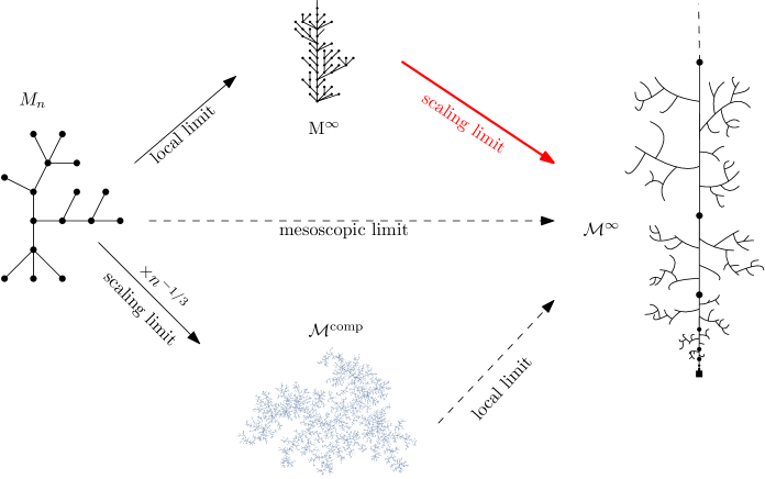
Figure 1: The objects $M_{n}$, $\mathcal{M}^{\mathrm{comp}}$, $\mathrm{M}^{\infty}$ and $\mathcal{M}^{\infty}$ and their relationships. This paper focuses on the red arrow. The solid black arrows are already proved in the literature, and the dashed ones are conjectured.

1.1 Structure of the root component of the WMSF of the PWIT

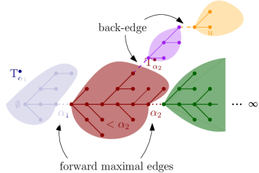
(a) Decomposition of the invasion percolation tree $\mathrm{T}^{\infty}$ into ponds that are linked along an infinite spine by forward maximal edges, drawn in dotted line. The edges in the dark red pond $\mathrm{T}_{\alpha_{2}}^{\bullet}$ all have weight smaller than $\alpha_{2}$, the forward maximal edge that exits it.

(b) Decomposition of the invasion percolation tree $T(u)$ into ponds. The invasion percolation starting from $u$ explores the orange pond first, then the purple one and the dark red one. The rest of the invasion coincides with that of the root from there.

Figure 2: Structure of invasion percolation clusters on the PWIT

First we describe the objects of study. Let $\mathbb{U}$ be the Ulam-Harris tree; this is the tree with vertex set $V(\mathbb{U})=\bigcup_{k\geq 0}\mathbb{N}^{k}$, and for each $k\geq 1$ and each vertex $v=(n_{1},\dots,n_{k})\in\mathbb{N}^{k}$ , an edge between $v$ and its parent $(n_{1},\dots,n_{k-1})$. For each $v=(n_{1},\dots,n_{k})\in\mathbb{U}$ , let $(x_{i},i\geq 1)$ be the atoms of a homogeneous rate one Poisson process on $\mathopen{[}0\mathclose{}\mathpunct{},\infty\mathclose{)}$, and for each $i\geq 1$ give the edge from $v$ to its child $v_{i}=(n_{1},\dots,n_{k},i)$ the weight $W({v,v_{i}})=x$. Writing $W=\{W(e),e\in E(\mathbb{U})\}$, where $E(\mathbb{U})$ is the edge set of $\mathbb{U}$ , the Poisson-weighted infinite tree is the tree $\mathbb{U}$ rooted at $\emptyset$, endowed with the weight function $W$, which we write as a triple $(\mathbb{U},\emptyset,W)$.

Invasion percolation, forward maximal edges and ponds.

Invasion percolation (also called Prim’s algorithm) on a rooted locally finite weighted graph with distinct weights is defined as follows: the algorithm grows a component from the root of the graph, adding at each step the lowest weight edge leaving the current component. When performed on a finite connected weighted graph, this procedure yields the minimal spanning tree of that graph. Performed on an infinite graph however, it yields an infinite tree whose set of vertices is a proper subset of the original graph, which we call the invasion percolation cluster of the root.

We consider $\mathrm{T}^{\infty}$ the invasion cluster of the root of the weighted rooted tree $(\mathbb{U},\emptyset,W)$. It is known that $\mathrm{T}^{\infty}$ is almost surely one-ended and that it admits a decomposition into ponds, by cutting at so-called forward maximal edges. We say that an edge $e\in E(\mathrm{T}^{\infty})$ is forward maximal if it disconnects the root $\emptyset$ from infinity and is such that if there exists $e^{\prime}\in E(\mathrm{T}^{\infty})$ such that $e$ is in the path joining $\emptyset$ and $e^{\prime}$ then $W(e^{\prime})<W(e)$. In terms of the invasion percolation process described above, this means that any edge explored after $e$ will have a smaller weight than $e$.

Denote by $\alpha_{1}>\alpha_{2}>\dots$ the respective weights of the successive forward maximal edges $e_{1},e_{2},\dots$ in the order in which they are discovered by the invasion percolation process, and denote by $\mathscr{A}=\{\alpha_{1},\alpha_{2},\dots\}$ the set of all their values. We can remove those edges in order to disconnect $\mathrm{T}^{\infty}$ into finite connected components that we call ponds. We denote those ponds by $(\mathrm{T}^{\bullet}_{\alpha})_{\alpha\in\mathscr{A}}$, by indexing them by the weight of the corresponding forward maximal edge exiting the component, which we call the type (called activation time in [25]) of the vertices belonging to the corresponding pond. Here, each $\mathrm{T}^{\bullet}_{\alpha}$ is then a finite rooted tree, rooted at its vertex closest to the root and pointed at the vertex from which the next forward maximal edge exits. See Figure 2 for an illustration.

Invasion percolation from every vertex.

For any vertex $u\in V(\mathbb{U})$, we can repeat the procedure above from vertex $u$ by just considering $T(u)$ the invasion percolation cluster of the rooted weighted tree $\mathbb{U}(u)=(U,u,W)$, the PWIT re-rooted at vertex $u$. Let $\widetilde{\mathrm{M}}$ be the union of all the trees $(T(u),u\in V(\mathbb{U}))$. The forest $\widetilde{\mathrm{M}}$ is the so-called Wired Minimal Spanning Forest of the PWIT. Now the tree $\mathrm{M}^{\infty}$, which we study in this paper, is defined as the connected component of the forest $\widetilde{\mathrm{M}}$ containing the root $\emptyset$ of $\mathbb{U}$. It is almost surely one-ended, see [2, Corollary 7.2].

The tree $\mathrm{M}^{\infty}$ of course contains $\mathrm{T}^{\infty}=T(\emptyset)$, the invasion percolation cluster of the root. Consider a vertex $u\in V(\mathbb{U})$ that is such that $u\notin\mathrm{T}^{\infty}$ and its invasion percolation cluster $T(u)$. The tree $T(u)$ can be disconnected along its own forward maximal edges in the same way as $T(\emptyset)$. Now if we suppose that $u\in\mathrm{M}^{\infty}$ then the facts that $T(\emptyset)$ and $T(u)$ are one-ended, as well as $\mathrm{M}^{\infty}$, imply that the ponds and forward maximal edges of $T(\emptyset)$ and $T(u)$ coincide except for a finite number of them: this ensures that the invasion percolation process from vertex $u$ visits a finite number of ponds before starting to explore one of the ponds $(\mathrm{T}^{\bullet}_{\alpha})_{\alpha\in\mathscr{A}}$. In order to avoid confusion, for $u\in\mathrm{M}^{\infty}$, we call any of the forward maximal edges of $T(u)$ that is not a forward maximal edge of $T(\emptyset)$ a back-edge. Any pond of $T(u)$ that does not overlap with $\mathrm{T}^{\infty}$ is denoted by $T_{\beta}$, where $\beta$ is the weight of the first back-edge visited by invasion percolation started from that vertex. Again we say that all the vertices in $T_{\beta}$ have type $\beta$.

Now, consider $\mathrm{M}^{\infty}$ and as before we disconnect it along the forward maximal edges $e_{1},e_{2}\dots$ of $\mathrm{T}^{\infty}$. We denote by $(\mathrm{M}^{\bullet}_{\alpha})_{\alpha\in\mathscr{A}}$ the obtained sequence of connected components. Each of those component $\mathrm{M}^{\bullet}_{\alpha}$ can actually be decomposed again into the union of $\mathrm{T}^{\bullet}_{\alpha}$ and a set of trees $T_{\beta}$ connected to each other along a tree structure by back-edges. In fact, $\mathrm{M}^{\bullet}_{\alpha}$ can be obtained from $\mathrm{T}^{\bullet}_{\alpha}$ by running the so-called Poisson–Galton–Watson Aggregation Process which we recall in Section 3. The idea of this paper is to define a similar structure in the continuum and prove that it is indeed the scaling limit of $\mathrm{M}^{\infty}$, resp. $\mathrm{T}^{\infty}$.

1.2 Summary of the results

Figure 3: Construction of the non-compact continuous object $\mathcal{M}^{\infty}$ (on the bottom) from a Poisson point process $\mathscr{P}$ (on top). The color of the trees below correspond to the atoms of the PPP above. Note that in $\mathscr{P}$ there is an accumulation of atoms near $\infty$ (not represented here).

We define an infinite one-ended continuum random tree $\mathcal{M}^{\infty}$ jointly with $\mathcal{T}^{\infty}\subset\mathcal{M}^{\infty}$, which are the continuous analogues of respectively $\mathrm{M}^{\infty}$ and $\mathrm{T}^{\infty}$.

Joint construction of $\mathcal{T}^{\infty}$ and $\mathcal{M}^{\infty}$.

We first explain how we can describe the object $\mathcal{M}^{\infty}$ from another object that we denote by $\mathcal{M}^{\bullet}$, which we then discuss below. This is slightly analogous to the construction of Brownian motion by chaining of excursions sampled from the Ito measure, though in our construction each component has another one immediately following it (among other differences). Let

• $\mathscr{P}$ be a Poisson Point Process on $\mathopen{(}0\mathclose{}\mathpunct{},\infty\mathclose{)}$ with intensity $\frac{1}{t}\mathrm{d}t$,

• $\left((\mathcal{T}^{\bullet}_{x},\mathcal{M}^{\bullet}_{x}),\ x\in\mathscr{P}\right)$ a collection of random variables, where conditionally on $\mathscr{P}$ they are independent and we have

  $$(\mathcal{T}^{\bullet}_{x},\mathcal{M}^{\bullet}_{x})\overset{(d)}{=}\left(\mathrm{Scale}(x^{-1},x^{-2};\mathcal{T}^{\bullet}),\ \mathrm{Scale}(x^{-1},x^{-3};\mathcal{M}^{\bullet})\right),$$

  where $(\mathcal{T}^{\bullet},\mathcal{M}^{\bullet})$ is a couple of random pointed rooted measured trees such that $\mathcal{T}^{\bullet}\subset\mathcal{M}^{\bullet}$ that we will describe in more details later on.

Then $\mathcal{M}^{\infty}$ is constructed from the sequence $(\mathcal{M}_{x}^{\bullet})_{x\in\mathscr{P}}$ as

$$\mathrm{Chain}(\mathcal{M}_{x}^{\bullet},\ x\in\mathscr{P}).$$

The tree $\mathcal{T}^{\infty}$ is constructed in a similar manner from $(\mathcal{T}_{x}^{\bullet})_{x\in\mathscr{P}}$ and can be seen as a subset of $\mathcal{M}^{\infty}$. The $\mathrm{Chain}$ construction will be defined in detail in Section 2, but essentially consists in taking all the sequence of rooted pointed trees $(\mathcal{M}_{x}^{\bullet})_{x\in\mathscr{P}}$ and gluing them head to tail in decreasing order of $x$-value. The resulting space is completed by adding an extra point $\rho_{\infty}$ which is characterized by $\rho_{\infty}:=\lim_{x\rightarrow\infty,x\in\mathscr{P}}\rho_{x}$, where for any $x\in\mathscr{P}$, the point $\rho_{x}$ denotes the common root of $\mathcal{T}^{\bullet}_{x}$ and $\mathcal{M}^{\bullet}_{x}$. The obtained space is an unbounded complete measured tree, rooted at $\rho_{\infty}$.

Notice the similar structure to that of $(\mathrm{T}^{\infty},\mathrm{M}^{\infty})$: the point process $\mathscr{P}$ corresponds to the set $\mathscr{A}$ of weights of forward maximal edges, the trees $(\mathcal{T}^{\bullet}_{x},\mathcal{M}^{\bullet}_{x})$ for $x\in\mathscr{P}$ take the place of the $(\mathrm{T}_{\alpha}^{\bullet},\mathrm{M}_{\alpha}^{\bullet})$ for $\alpha\in\mathscr{A}$, and the Chain construction mimics the way that we can get $\mathrm{M}^{\infty}$ and $\mathrm{T}^{\infty}$ from linking all the $(\mathrm{M}_{\alpha}^{\bullet})_{\alpha\in\mathscr{A}}$ (resp. the $(\mathrm{T}_{\alpha}^{\bullet})_{\alpha\in\mathscr{A}}$) using the forward maximal edges.

Convergence results.

Before discussing the construction of $(\mathcal{T}^{\bullet},\mathcal{M}^{\bullet})$, which are the building blocks of $\mathcal{T}^{\infty}$ and $\mathcal{M}^{\infty}$, we state our scaling limit convergence result. The result below is expressed in the local Gromov–Hausdorff–Prokhorov topology, the definition of which is recalled in Section 2. The tree $\mathcal{M}^{\infty}$ is the scaling limit of $\mathrm{M}^{\infty}$ for the local Gromov-Hausdorff-Prokhorov topology. More precisely

$$\mathrm{Scale}\left(r,\frac{r^{3}}{C_{0}};\mathrm{M}^{\infty}\right)\underset{r\rightarrow 0}{\rightarrow}\mathcal{M}^{\infty},$$

where the constant $C_{0}$ is defined later in (47). The above convergence happens jointly with

$$\mathrm{Scale}\left(r,r^{2};\mathrm{T}^{\infty}\right)\underset{r\rightarrow 0}{\rightarrow}\mathcal{T}^{\infty}.$$

Note that invasion percolation on a $d$-regular tree and its scaling limit were investigated in [11]. While the behavior does not depend significantly on $d$, the extension to the PWIT was only investigated later in [5]. In [11], the tree generated by the invasion percolation process started at the root is studied using its encoding via functions such as the contour function, height function or Lukasiewicz path. The scaling limit is then described as well by its encoding by a height function that is described as the solution to some stochastic differential equation. Heuristically, the obtained tree should have the same distribution as $\mathcal{T}^{\infty}$, up to some deterministic scaling, even though our description can seem quite different as first glance.

Construction of $\mathcal{M}^{\bullet}$ from $\mathcal{T}^{\bullet}$: the Brownian tree aggregation process.

We now describe in more details the distribution of the pair $(\mathcal{T}^{\bullet},\mathcal{M}^{\bullet})$ used to construct $\mathcal{T}^{\infty}$ and $\mathcal{M}^{\infty}$. They are seen as (nested) random metric spaces, endowed with a common root $\rho$ and distinguished point $v$, and measures (one for each) that are not necessarily normalized to be probability measures.

First, $\mathcal{T}^{\bullet}$ has the distribution of a Brownian tree with random mass $X$, where $X\overset{(d)}{=}\sqrt{2}\cdot\Gamma$ where $\Gamma$ has distribution $\mathrm{Gamma}(\frac{1}{2})$, endowed with a randomly chosen point $v$ (on top of being rooted at some point $\rho$). The construction of $\mathcal{M}^{\bullet}$ from $\mathcal{T}^{\bullet}$ then uses a process that we call the Brownian tree aggregation process (which is analogous to the Poisson-Galton-Watson aggregation process used in the discrete setting to describe the construction of $\mathrm{M}_{\alpha}^{\bullet}$ for any $\alpha>1$). A useful analogy for the reader is the stick-breaking construction of the CRT, where line segments of random lengths are glued at uniform points on the union of all past segments. However, unlike that process, there are infinitely many attached trees being added in any time interval.

Here is a first intuitive way of understanding the construction of $\mathcal{M}^{\bullet}$. This is a growth process for a tree, started at time $t=1$ (which turns out to be more convenient) with the seed $\mathcal{T}^{\bullet}$. Immediately after time $t=1$, independent Brownian trees arrive and are attached to the existing tree by having their root identified to a point already present. At time $t$, attachments of trees of mass $y$ to an element of mass $\mathrm{d}m$ of the current structure arrive at rate

$$\frac{1}{\sqrt{2\pi}y^{3/2}}\exp\left(-\frac{t^{2}}{2}y\right)\mathrm{d}y\mathrm{d}m,$$ (1)

where each corresponding tree of mass $y$ is a Brownian tree with the given mass (conditionally on all the rest). The object $\mathcal{M}^{\bullet}$ is the limit as $t\to\infty$ of the process defined above, still rooted and pointed at respectively $\rho$ and $v$.

The way that we define such a process formally deviates slightly from this intuition, and start with the process giving the total mass of the tree at time $t$. We would like to define a pure jump Markov process $(\mathcal{W}_{t})_{t\geq 1}$ in terms of its generator. Since this Markov process is inhomogeneous in time, we actually give the generator of the process $((t,\mathcal{W}_{t}))_{t\geq 1}$, which is time-homogeneous. The generator $\mathbf{A}$ of the process $(t,\mathcal{W}_{t})$ is so that for any smooth and compactly supported function $f:(0,\infty)\times\mathopen{(}0\mathclose{}\mathpunct{},\infty\mathclose{)}\rightarrow\mathbb{R}$ we have

$$\mathbf{A}f(t,x)=\partial_{t}f(t,x)+x\cdot\int_{0}^{\infty}\left(f(t,x+y)-f(t,x)\right)\frac{\exp\left(-\frac{t^{2}}{2}y\right)}{y^{\frac{3}{2}}\sqrt{2\pi}}\mathrm{d}y.$$ (2)

This process represent the evolution of the total mass that is present at time $t$. The process $(\mathcal{W}_{t})_{t\geq 1}$ is a subordinator and a pure jump process, and so has countably many jumps. For every jump time $t$ of the process, take an independent Brownian tree

$$\mathcal{T}_{t}$$

with mass given by the size of the jump $w_{t}:=\mathcal{W}_{t}-\mathcal{W}_{t-}$. For every such times $t$, a point $X_{t}$ is sampled proportionally to the mass measure on

$$\mathcal{T}^{\bullet}\sqcup\bigsqcup_{1<s<t}\mathcal{T}_{t}.$$ (3)

The tree at time $t$ is obtained by gluing the root of every $\mathcal{T}_{s}$, for all jump times $s\leq t$ of the process $\mathcal{W}$, to the corresponding point $X_{s}$. For $t=\infty$, we take the completion of the obtained space. The fact that this construction makes sense and almost surely yields a compact metric space is proved in a more general setting in the corresponding section.

We should also mention how the measure on $\mathcal{M}^{\bullet}$ is obtained: The total mass of the tree constructed up to time $t$ is $\mathcal{W}_{t}$ and tends to infinity. The measure on $\mathcal{M}^{\bullet}$ arises as the scaling limit as $t\to\infty$ of the mass-measure on the trees that have index less than $t$. As it turns out, the correct normalization is $\frac{1}{t}$. The measure $\mu$ on $\mathcal{M}^{\bullet}$ is defined as $\mu:=\lim_{t\rightarrow\infty}\frac{1}{t}\mu_{t}$, where $\mu_{t}$ is the measure on the tree at time $t$, and the limit is a weak limit of measures. The limiting measure on $\mathcal{M}^{\bullet}$ has total mass given by

$$Y:=\lim_{t\to\infty}\frac{\mathcal{W}_{t}}{t}.$$

More about that in Section 3.

Thanks to the construction of $\mathcal{M}^{\bullet}$ as an aggregation process, we can determine some of its geometric properties. The random metric space $\mathcal{M}^{\bullet}$ is well-defined as a random variable in $\mathbb{L}^{\bullet,c}$. Furthermore

1. Its mass and diameter have moments of all orders.

2. It almost surely has Minkowski and Hausdorff dimension $3$.

3. Its measure is almost surely non-zero, diffuse and has full support.

Note that, as a result, the non-compact random metric space $\mathcal{M}^{\infty}$ which is a countable union of copies of $\mathcal{M}^{\bullet}$ also has Hausdorff dimension $3$ and diffuse mass measure with full support.

1.3 Organization of this paper

We start in Section 2 by recalling some facts about the Gromov–Hausdorff–Prokhorov topology and introducing the two constructions called $\mathrm{Chain}$ and aggregation process ($\mathrm{Aggreg}$) respectively. These constructions are particularly important because we interpret all our objects in this framework. In particular, we state some sufficient conditions for the convergence of such structures. In Section 3 we then use these constructions to rigorously construct the trees $\mathcal{M}^{\bullet}$ and $\mathcal{M}^{\infty}$. In particular, we prove Theorem 1.2 in Section 3.1. Then in Section 4, we study the tree $\mathrm{M}^{\infty}$ and decompose it in a way that use again the $\mathrm{Chain}$ and $\mathrm{Aggreg}$ constructions in an analogous way. We then prove Theorem 1.2 in Section 4.8 by using results from Section 2 that ensure that the limit of objects constructed as a $\mathrm{Chain}$ (resp. $\mathrm{Aggreg}$) of discrete objects can be described as a $\mathrm{Chain}$ (resp. $\mathrm{Aggreg}$) of continuous ones.

Table 1: Table of notation of the main objects of the paper

Discrete objects
$\mathscr{A}$	:	set of weights of forward maximal edges of $\mathrm{T}^{\infty}$
$\mathrm{T}^{\infty}$	:	invasion percolation cluster of the root of the PWIT
$\mathrm{T}_{\alpha}^{\bullet}$	:	defined for $\alpha\in\mathscr{A}$; it is the pond located just before the forward maximal edge of weight $\alpha$
$M_{n}$	:	minimal spanning tree of $K_{n}$ endowed with independent random weights
$\mathrm{M}^{\infty}$	:	the root component of the WMSF of the PWIT
$\mathrm{M}_{\alpha}^{\bullet}$	:	the connected component of $\mathrm{M}^{\infty}$ after removing the forward maximal edges of $\mathrm{T}^{\infty}$ that contains $\mathrm{T}_{\alpha}^{\bullet}$
Continuous objects
$\mathscr{P}$	:	Poisson point process on $\mathopen{(}0\mathclose{}\mathpunct{},\infty\mathclose{)}$ with intensity measure $\frac{\differential t}{t}$
$\mathcal{T}^{\infty}$	:	scaling limit of $\mathrm{T}^{\infty}$
$\mathcal{T}^{\bullet}$	:	scaling limit of $\mathrm{T}_{\alpha}^{\bullet}$
$\mathcal{M}^{\infty}$	:	scaling limit of $\mathrm{M}^{\infty}$
$\mathcal{M}^{\bullet}$	:	scaling limit of $\mathrm{M}_{\alpha}^{\bullet}$
$(\mathcal{W}_{t})_{t\geq 1}$	:	weight process used in the construction of $\mathcal{M}^{\bullet}$
$X$	:	total mass of $\mathcal{T}^{\bullet}$ and starting value of $(\mathcal{W}_{t})_{t\geq 1}$, i.e. $X=\mathcal{W}_{1}$
$Y$	:	total mass of $\mathcal{M}^{\bullet}$, obtained as $Y=\lim_{t\rightarrow\infty}\frac{\mathcal{W}_{t}}{t}$
$\mathscr{J}$	:	set of jumps of the weight process $(\mathcal{W}_{t})_{t\geq 1}$
$(w_{t})_{t\in\mathscr{J}}$	:	jumps $w_{t}=\mathcal{W}_{t}-\mathcal{W}_{t-}$ of the weight process
$\mathcal{T}_{t}$	:	Brownian CRT with total mass $w_{t}$
Constructions
$\mathrm{mass}(\mathsf{X})$	:	total mass of the measure carried by the metric measured space $\mathsf{X}$
$\mathrm{diam}(\mathsf{X})$	:	diameter of the metric (possibly measured) space $\mathsf{X}$
$\mathrm{Scale}(a,b;\mathsf{X})$	:	version of the metric measured space $\mathsf{X}$ where the distances are scaled by $a$ and the mass is scaled by $b$
$\mathrm{Chain}$	:	construction taking a sequence of length spaces and linking them, each one to the next
$\mathrm{Aggreg}$	:	construction that yields a metric space from the result of an aggregation process
$\mathbb{L}$	:	set of equivalence classes of rooted, measured, locally compact length spaces
$\mathbb{L}^{c}$	:	set of equivalence classes of rooted, measured, compact length spaces
$\mathbb{L}^{\bullet,c}$	:	set of equivalence classes of rooted, pointed, measured, compact length spaces
Other symbols
$C_{0}$	:	some positive constant defined in (47)
$r$	:	positive parameter destined to tend to $0$
$\operatorname{cst}$	:	a positive constant whose value may change along the lines

2 Constructions and convergences

In this section, we introduce two constructions from sequences of measured metric space. One of them is fairly simple and consists in linking a sequence of metric spaces in a linear manner: we call it the chain construction. The other one is slightly more involved and consists of gluing some ordered family of metric spaces on top of each other in a random way: this is called an aggregation process. It is a natural extension of the so called "line-breaking" construction of random trees [7, 8, 16], already extended to more general metric spaces [17, 27], where we do not constrain the blocks that we glue together to arrive in a discrete order anymore.

We state some properties of these two constructions (in particular convergence results) and we explain how to interpret our objects of interest in this setting. These results will be the base of the rest of our arguments.

In this section we only expose results and give an idea of how they are used later in the paper. The proofs of the results stated here will be postponed to the Appendix.

2.1 Reminder about the pointed GH and GHP topologies and local versions

In this section, we give a brief reminder about the definition of the Hausdorff, Gromov–Hausdorff and Gromov–Hausdorff–Prokhorov topologies on compact metric spaces, and their local equivalent on boundedly finite rooted metric spaces. We will mainly follow the exposition of [1]. This section can be skipped at first reading.

Let $(X,d^{X})$ be a Polish metric space and ${\mathcal{B}}(X)$ be its set of Borel measurable subsets. The diameter of $A\in{\mathcal{B}}(X)$ is given by:

$$\operatorname{diam}(A)=\sup\left\{d^{X}(x,y)\mathrel{}\middle|\mathrel{}x,y\in A\right\}.$$

For $A,B\in{\mathcal{B}}(X)$, we set:

$$d_{\text{H}}^{X}(A,B)=\inf\{\epsilon>0;\ A\subset B^{\epsilon}\ \mathrm{and}\ B\subset A^{\epsilon}\},$$

the Hausdorff distance between $A$ and $B$, where

$$A^{\epsilon}=\left\{x\in X\mathrel{}\middle|\mathrel{}\inf_{y\in A}d^{X}(x,y)<\epsilon\right\}$$ (4)

is the $\epsilon$- fattening of $A$. If $(X,d^{X})$ is compact, then the space of compact subsets of $X$, endowed with the Hausdorff distance, is compact.

Let $\mathrm{Mes}_{f}(X)$ denote the set of all finite Borel measures on $X$. If $\mu,\nu\in\mathrm{Mes}_{f}(X)$, we set:

$$d_{\text{P}}^{X}(\mu,\nu)=\inf\left\{\epsilon>0\mathrel{}\middle|\mathrel{}\mu(A)\leq\nu(A^{\epsilon})+\epsilon\text{ and }\nu(A)\leq\mu(A^{\epsilon})+\epsilon\ \text{ for any closed set }A\right\},$$

the Prokhorov distance between $\mu$ and $\nu$. It is well known, that $(\mathrm{Mes}_{f}(X),d_{\text{P}}^{X})$ is a Polish metric space, and that the topology generated by $d_{\text{P}}^{X}$ is exactly the topology of weak convergence.

The notion of Prokhorov distance can be extended in the following way. A Borel measure is said to be locally finite if the measure of any bounded Borel set is finite. Let $\mathrm{Mes}(X)$ denote the set of all locally finite Borel measures on $X$. Let $\rho$ be a distinguished element of $X$, which we call the root. We consider the closed ball of radius $R$ centered at $\rho$:

$$X^{(R)}=\left\{x\in X\mathrel{}\middle|\mathrel{}d^{X}(\rho,x)\leq R\right\},$$ (5)

and for $\mu\in\mathrm{Mes}(X)$ its restriction $\mu^{(R)}$ to $X^{(R)}$:

$$\mu^{(R)}(dx)=\mathbf{1}_{X^{(R)}}(x)\;\mu(dx).$$ (6)

If $\mu,\nu\in\mathrm{Mes}(X)$, the generalized Prokhorov distance between $\mu$ and $\nu$ is defined as:

$$d_{\text{gP}}^{X}(\mu,\nu)=\int_{0}^{\infty}\exp{-R}\left(1\wedge d^{X}_{\text{P}}\left(\mu^{(R)},\nu^{(R)}\right)\right)\ \differential R.$$ (7)

The function $d_{\text{gP}}^{X}$ is well defined and is a distance. Furthermore $(\mathrm{Mes}(X),d_{\text{gP}}^{X})$ is a Polish metric space, and the topology generated by $d_{\text{gP}}^{X}$ is exactly the topology of vague convergence. When there is no ambiguity on the metric space $(X,d^{X})$, we may write $d$, $d_{\text{H}}$, and $d_{\text{P}}$ instead of $d^{X}$, $d^{X}_{\text{H}}$ and $d^{X}_{\text{P}}$.

If $\Phi:X\rightarrow X^{\prime}$ is a Borel-measurable map between two Polish metric spaces and if $\mu$ is a Borel measure on $X$, we will note $\Phi_{*}\mu$ the image measure on $X^{\prime}$ defined by $\Phi_{*}\mu(A)=\mu(\Phi^{-1}(A))$, for any Borel set $A\subset X$.

Definition .

• A rooted measured metric space $\mathsf{X}=(X,d,\rho,\mu)$ is a metric space $(X,d)$ with a distinguished element $\rho\in X$, called the root, and a locally finite Borel measure $\mu$.

• Two rooted measured metric spaces $\mathsf{X}=(X,d,\rho,\mu)$ and $\mathsf{X}^{\prime}=(X^{\prime},d^{\prime},\rho^{\prime},\mu^{\prime})$ are said to be GHP-isometric if there exists an isometric one-to-one map $\Phi:X\rightarrow X^{\prime}$ such that $\Phi(\rho)=\rho^{\prime}$ and $\Phi_{*}\mu=\mu^{\prime}$. In that case, $\Phi$ is called a GHP-isometry.

Notice that if $(X,d)$ is compact, then a locally finite measure on $X$ is finite and belongs to $\mathrm{Mes}_{f}(X)$. We will now use a procedure due to Edwards [15] and developed by Gromov [18] to compare any two compact rooted measured metric spaces, even if they are not subspaces of the same Polish metric space.

2.1.1 Gromov-Hausdorff-Prokhorov metric for compact spaces

Let $(X,d)$ and $(X^{\prime},d^{\prime})$ be two compact metric spaces. The Gromov-Hausdorff metric between $(X,d)$ and $(X^{\prime},d^{\prime})$ is given by:

$$d_{\text{GH}}^{c}((X,d),(X^{\prime},d^{\prime}))=\inf_{\varphi,\varphi^{\prime},Z}d_{\text{H}}^{Z}(\varphi(X),\varphi^{\prime}(X^{\prime})),$$ (8)

where the infimum is taken over all isometric embeddings $\varphi:X\hookrightarrow Z$ and $\varphi^{\prime}:X^{\prime}\hookrightarrow Z$ into some common Polish metric space $(Z,d^{Z})$. The last display actually defines a metric on the set of isometry classes of compact metric spaces.

Now, we introduce the Gromov–Hausdorff–Prokhorov distance for compact spaces. Let $\mathsf{X}=(X,d,\rho,\mu)$ and $\mathsf{X}^{\prime}=(X^{\prime},d^{\prime},\rho^{\prime},\mu^{\prime})$ be two compact rooted measured metric spaces, and define:

$$d_{\mathrm{GHP}}^{c}(\mathsf{X},\mathsf{X}^{\prime})=\inf_{\Phi,\Phi^{\prime},Z}\left(d^{Z}(\Phi(\rho),\Phi^{\prime}(\rho^{\prime}))+d_{\text{H}}^{Z}(\Phi(X),\Phi^{\prime}(X^{\prime}))+d_{\text{P}}^{Z}(\Phi_{*}\mu,\Phi_{*}^{\prime}\mu^{\prime})\right),$$ (9)

where the infimum is taken over all isometric embeddings $\Phi:X\hookrightarrow Z$ and $\Phi^{\prime}:X^{\prime}\hookrightarrow Z$ into some common Polish metric space $(Z,d^{Z})$.

Note that equation (9) does not actually define a distance, as $d_{\mathrm{GHP}}^{c}(\mathsf{X},\mathsf{X}^{\prime})=0$ if $\mathsf{X}$ and $\mathsf{X}^{\prime}$ are GHP-isometric. Therefore, we shall consider $\mathbb{K}$, the set of GHP-isometry classes of compact rooted measured metric space and identify a compact rooted measured metric space with its class in $\mathbb{K}$. Then the function $d_{\mathrm{GHP}}^{c}$ is finite on $\mathbb{K}^{2}$.

[Theorem 2.5 of [1]]

• The function $d_{\mathrm{GHP}}^{c}$ defines a distance on $\mathbb{K}$.

• The space $(\mathbb{K},d_{\mathrm{GHP}}^{c})$ is a Polish metric space.

The function $d_{\mathrm{GHP}}^{c}$ is called the Gromov–Hausdorff–Prokhorov distance. The Gromov–Hausdorff–Prokhorov distance could be defined without reference to any root. However, the introduction of the root is necessary to extend the definition of the Gromov–Hausdorff–Prokhorov distance to spaces that are not necessarily compact.

We sometimes need to endow our spaces with extra structure, like an additional distinguished point for example. In that case, it is possible to modify the definition of the Gromov–Hausdorff–Prokhorov distance to account for this extra piece of data and the corresponding space $\mathbb{K}^{\bullet}$ of equivalence classes of root pointed compact metric spaces is also Polish. We denote by $d_{\mathrm{GHP}}^{\bullet,c}$ the corresponding distance.

2.1.2 Gromov–Hausdorff–Prokhorov distance for locally compact length spaces

A metric space $(X,d)$ is a length space if for every $x,y\in X$ , we have $d(x,y)=\inf\{\mathrm{Len}(\gamma)\}$, - where the infimum is taken over all rectifiable curves $\gamma:\mathopen{[}0\mathclose{}\mathpunct{},1\mathclose{]}\rightarrow X$ such that $\gamma(0)=x$ and $\gamma(1)=y$ , and where $\mathrm{Len}(\gamma)$ is the length of the rectifiable curve $\gamma$.

Let $\mathbb{L}$ be the set of GHP-isometry classes of rooted, measured, complete and locally compact length spaces and identify a rooted, measured, complete and locally compact length space with its class in $\mathbb{L}$. We will also denote by $\mathbb{L}^{c}=\mathbb{K}\cap\mathbb{L}$, and $\mathbb{L}^{\bullet,c}$ for the space of their pointed counterparts.

If $\mathsf{X}=(X,d,\rho,\mu)\in\mathbb{L}$, then for $R\geq 0$ we will consider its restriction to the closed ball of radius $R$ centered at $\rho$, denoted by $\mathsf{X}^{(R)}=(X^{(R)},d^{(R)},\rho^{(R)},\mu^{(R)})$, where $X^{(R)}$ is defined by (5), the distance $d^{(R)}$ is the restriction of $d$ to $X^{(R)}$, and the measure $\mu^{(R)}$ is defined by (6). If $\mathsf{X}$ belongs to $\mathbb{L}$ , then $\mathsf{X}^{(R)}$ belongs to $\mathbb{K}$ for all $R\geq 0$.

The following distance is well defined on $\mathbb{L}\times\mathbb{L}$:

$$d_{\mathrm{GHP}}(\mathsf{X},\mathsf{Y})=\int_{0}^{\infty}e^{-R}\cdot\left(1\wedge d^{c}_{\mathrm{GHP}}\left(\mathsf{X}^{(R)},\mathsf{Y}^{(R)}\right)\right)\differential R.$$

The weight $e^{-R}$ and truncation are arbitrary and their choice does not affect the resulting topology.

[Theorem 2.9 and Proposition 2.10 of [1]] We have the following:

• The function $d_{\mathrm{GHP}}$ defines a distance on $\mathbb{L}$.

• The space $(\mathbb{L},d_{\mathrm{GHP}})$ is a Polish metric space.

• The two distances $d_{\mathrm{GHP}}$ and $d_{\mathrm{GHP}}^{c}$ define the same topology on $\mathbb{K}\cap\mathbb{L}$.

All the objects that we study in this paper can be understood in that context of length spaces. The discrete objects that we are considering (discrete trees) can be seen as length spaces by considering their cable graph, meaning that we consider every edge in the tree as a segment of length $1$. The continuous objects that we are considering are all weak limits of such discrete objects that are indeed length spaces. This makes them length spaces as well by the fact that taking Gromov–Hausdorff limits preserves the property of being a length space, see [13, Theorem 7.5.1].

2.2 The chain construction

In this section, we present a construction that takes a family of compact measured metric spaces and glues them sequentially along a path.

2.2.1 Construction

Suppose that we are given a discrete set $\mathscr{N}\subset\mathopen{(}0\mathclose{}\mathpunct{},\infty\mathclose{)}$ and a family $(\mathsf{L}_{t}^{\bullet},t\in\mathscr{N})$ of rooted pointed measured compact length spaces indexed by the set $\mathscr{N}$, where

$$\mathsf{L}_{t}^{\bullet}=(L_{t},d_{t},\rho_{t},v_{t},\nu_{t}).$$

We would like to make sense of the object obtained by linking every $\mathsf{L}_{t}^{\bullet}$ by identifying the distinguished point $v_{t}$ to the root $\rho_{t^{\prime}}$ of the next block in ascending order. For the result to be well defined we make the following assumptions.

Assume that

1. For any $A>0$ we have

   $$\sum_{t\in\mathscr{N}\cap\mathopen{(}A\mathclose{}\mathpunct{},\infty\mathclose{)}}d_{t}(\rho_{t},v_{t})<\infty\quad\text{ and }\quad\sum_{t\in\mathscr{N}\cap\mathopen{(}A\mathclose{}\mathpunct{},\infty\mathclose{)}}\nu_{t}(L_{t})<\infty$$

2. We have

   $$\sup_{t\in\mathscr{N}\cap\mathopen{(}A\mathclose{}\mathpunct{},\infty\mathclose{)}}\operatorname{diam}(\mathsf{L}_{t}^{\bullet})\underset{A\rightarrow\infty}{\rightarrow}0.$$

3. For any $\epsilon>0$, one of the two following conditions is satisfied:

   1. $\sum_{t\in\mathscr{N}\cap\mathopen{(}0\mathclose{}\mathpunct{},\epsilon\mathclose{)}}d_{t}(\rho_{t},v_{t})=\infty$,

   2. $\mathscr{N}\cap\mathopen{(}0\mathclose{}\mathpunct{},\epsilon\mathclose{)}$ is finite.

We define $L_{\infty}=\{\rho_{\infty}\}$ and consider

$$\bigsqcup_{t\in\mathscr{N}\cup\{\rho_{\infty}\}}L_{t}$$

which we endow with the pseudo-distance $d$ defined as

$$d(x,y)=d(y,x)=\begin{cases}d_{t}(x,y)&\text{if }x,y\in L_{t},\\ d_{t}(x,v_{t})+\displaystyle\sum_{r\in\mathscr{N}\cap(s,t)}d_{r}(\rho_{r},v_{r})+d_{s}(\rho_{s},y)&\text{if }(x,y)\in L_{s}\times L_{t},\ t<s.\end{cases}$$ (10)

Then $\mathrm{Chain}(\mathsf{L}_{t}^{\bullet},t\in\mathscr{N})$ is defined as

$$\left(\bigsqcup_{t\in\mathscr{N}\cup\{\rho_{\infty}\}}L_{t}\right)/\sim$$

where $\sim$ is the equivalence relation generated by $x\sim y$ if $d(x,y)=0$. The space $\mathrm{Chain}(\mathsf{L}_{t}^{\bullet},t\in\mathscr{N})$ is seen as a rooted measured metric space after endowing the space with the projection of the distance $d$ and the measure $\sum_{t\in\mathscr{N}}\nu_{t}$ and the root $\rho_{\infty}$.

Lemma .

If assumptions (Ch1), (Ch2), (Ch3) hold then $\mathrm{Chain}(\mathsf{L}_{t}^{\bullet},t\in\mathscr{N})$ is an element of $\mathbb{L}$.

The proof of this lemma can be found in Appendix A.

Remark .

If only (Ch3) fails, then a length space in $\mathbb{L}$ can still be constructed from $\mathrm{Chain}(\mathsf{L}_{t}^{\bullet},t\in\mathscr{N})$, except that it needs to be completed with a second point $\rho_{0}$ on the other side. Also, note that in our definition, we exclude the possibility that the set $\mathscr{N}$ could be dense. The construction could be made more general to accommodate for such situations, but this would require the addition of more (possibly an uncountable infinity) completion points in between the links of the chain. Such a construction appears for example in [30, Section 6.1].

2.2.2 Convergence of chains

In order to prove scaling limit convergence results for the discrete objects mentioned above to the continuous ones, we provide here sufficient conditions for convergence. Since we will consider convergence of random such objects, we state the condition for a random object constructed as $\mathrm{Chain}(\mathsf{L}_{t}^{\bullet,r},t\in\mathscr{N}^{r})$ to converge to a limit expressed as $\mathrm{Chain}(\mathsf{L}_{t}^{\bullet,0},t\in\mathscr{N}^{0})$ as $r\rightarrow 0$. We assume that for any $r\geq 0$, so in particular for $r=0$ as well, the point process $\mathscr{N}^{r}$ and the family $(\mathsf{L}_{t}^{\bullet,r},t\in\mathscr{N}^{r})$ satisfy (Ch1), (Ch2), (Ch3) almost surely. Additionally we assume the following:

1. The process $((t,\mathsf{L}_{t}^{\bullet,r}),\ t\in\mathscr{N}^{r})$ converges in distribution as $r\rightarrow 0$ to $((t,\mathsf{L}_{t}^{\bullet,0}),\ t\in\mathscr{N}^{0})$ as point processes on $\mathopen{(}0\mathclose{}\mathpunct{},\infty\mathclose{)}$ with marks in $\mathbb{L}^{\bullet,c}$. We mean by that that for any compact set $K\subset\mathopen{(}0\mathclose{}\mathpunct{},\infty\mathclose{)}$, the random measure

   $$\sum_{t\in\mathscr{N}^{r}\cap K}\delta_{(x,\mathsf{L}_{t}^{\bullet,r})}\overset{(d)}{\rightarrow}\sum_{t\in\mathscr{N}^{0}\cap K}\delta_{(x,\mathsf{L}_{t}^{\bullet,0})}$$

   as $r\rightarrow 0$ for the topology of the weak convergence of measures on $K\times\mathbb{L}^{\bullet,c}$.

2. For any $\epsilon>0$

   $$\limsup_{A\rightarrow\infty}\limsup_{r\rightarrow 0}\mathbb{P}\left(\mathrm{mass}\left(\mathrm{Chain}(\mathsf{L}_{t}^{\bullet,r},t\in\mathscr{N}^{r}\cap\mathopen{(}A\mathclose{}\mathpunct{},\infty\mathclose{)})\right)>\epsilon\right)=0.$$

3. For any $\epsilon>0$

   $$\limsup_{A\rightarrow\infty}\limsup_{r\rightarrow 0}\mathbb{P}\left(\mathrm{diam}\left(\mathrm{Chain}(\mathsf{L}_{t}^{\bullet,r},t\in\mathscr{N}^{r}\cap\mathopen{(}A\mathclose{}\mathpunct{},\infty\mathclose{)})\right)>\epsilon\right)=0.$$

Then we have the following result. Suppose that for all $r>0$, the family $(\mathsf{L}_{t}^{\bullet,r},t\in\mathscr{N}^{r})$ satisfies (Ch1), (Ch2) and (Ch3) almost surely. Additionally, assume that $(\mathsf{L}_{t}^{\bullet,0},t\in\mathscr{N}^{0})$ satisfies (Ch1), (Ch2) and (Ch3)(Ch3a) almost surely. Then, under (ChConv1),(ChConv2), (ChConv3), we have the following convergence in distribution in the space $\mathbb{L}$,

$$\mathrm{Chain}(\mathsf{L}_{t}^{\bullet,r},t\in\mathscr{N}^{r})\underset{r\rightarrow 0}{\rightarrow}\mathrm{Chain}(\mathsf{L}_{t}^{\bullet,0},t\in\mathscr{N}^{0}).$$

The proof of this proposition can be found in Appendix A.

2.3 Aggregation processes

The second construction that we will use is that of aggregation processes. In this case, we create a metric space by gluing together a (potentially infinite) collection of measured metric spaces $\left(\mathsf{B}_{t},\ t\in\mathscr{J}\right)$ in a random manner. The reader familiar with the stick-breaking construction of the CRT may wish to keep that in mind as a useful analogy. Indeed, the stick breaking construction can be defined as a special case of an aggregation process as defined here. However, unlike the stick breaking construction, here it is possible that infinitely many blocks are being glued within a finite time interval. (For any $t<\infty$ he blocks used up to time $t$ still have finite total mass.)

2.3.1 Construction

Since the definition of this process is a bit more involved, we express it for a particular case where the blocks $\left(\mathsf{B}_{t},t\in\mathscr{J}\right)$ that we glue together are random and satisfy some ad hoc assumptions that will be satisfied by the objects studied in this paper. We start with

• a weight process $(W_{t})_{t\geq t_{0}}$, which is a càdlàg increasing pure-jump process, such that $W_{t_{0}}>0$, (we denote by $\mathscr{J}$ its set of jump times),

• a seed $\mathsf{S}^{\bullet}=(S,\rho,v,d_{S},\nu_{S})$ which is a compact, rooted, pointed, measured length space (i.e. an element of $\mathbb{L}^{\bullet,c}$) and has total mass equal to $W_{t_{0}}$.

• a block-distribution family $\eta=\left(\eta(t,w):\ t>t_{0},w>0\right)$ of distributions on $\mathbb{L}^{c}$ which is such that for any $t>t_{0},w>0$, an object $\mathsf{B}(t,w)$ sampled under the measure $\eta(t,w)$ almost surely has mass $w$.

From these, we construct below some rooted (pointed) random metric space

$$\mathrm{Aggreg}((W_{t})_{t\geq t_{0}},\mathsf{S}^{\bullet},\eta).$$

For each jump time $t\in\mathscr{J}$ we let $w_{t}=W_{t}-W_{t-}$ and we let $w_{t_{0}}=W_{t_{0}}$. Then we sample a random block $\mathsf{B}_{t}=(B_{t},d_{t},\rho_{t},\nu_{t})$, whose distribution is $\eta(t,w_{t})$, independently for all $t\in\mathscr{J}$. Then the object of interest in constructed from the collection $\left(\mathsf{B}_{t},t\in\mathscr{J}\right)$, by quotienting the set

$$S\sqcup\bigsqcup_{t>t_{0}}B_{t},$$

by the appropriate identification of pairs of points: For every jump time $t\in\mathscr{J}$, we pick a random point $X_{t}$ on the set $\bigsqcup_{t_{0}\leq s<t}B_{s}$ using a normalized version of the measure $\sum_{t_{0}\leq s<t}\nu_{s}$. Define the equivalence relation $\sim$ as generated by the relations $X_{t}\sim\rho_{t}$ for each $t\in\mathscr{J}$. The object of interest is then the metric gluing

$$(A_{\infty},\rho,v,d):=\overline{\left(\mathsf{S}^{\bullet}\sqcup\bigsqcup_{t>t_{0}}\mathsf{B}_{t}\right)/\sim}$$

in the sense of [13], where the root $\rho$ and distinguished point $v$ are inherited from the seed $\mathsf{S}^{\bullet}$. The overline in the last display represent the operation of completion with respect to the distance defined by the metric gluing. Note that the completion and the gluing operation both preserve the property of being a length space. We will see below that under some reasonable assumptions, this space can be shown to be almost surely compact.

For any $t\geq t_{0}$, we can consider the probability measure $\mu_{t}:=W_{t}^{-1}\sum_{t_{0}\leq s\leq t}\nu_{s}$. Again, under some reasonable assumptions, this sequence of measures almost surely converge for the weak topology as $t\rightarrow\infty$ so that $A_{\infty}$ can be endowed with a probability measure $\mu_{\infty}:=\lim_{t\rightarrow\infty}\mu_{t}$. This makes

$$\mathrm{Aggreg}((W_{t})_{t\geq t_{0}},\mathsf{S}^{\bullet},\eta):=\mathsf{A}_{\infty}^{\bullet}=(A_{\infty},\rho,v,d,\mu_{\infty})$$

an element of $\mathbb{L}^{\bullet,c}$ almost surely. In what comes next we will work under the following two assumptions, which are satisfied in all the cases studied in this paper.

1. For some deterministic non-increasing function $\delta:\mathopen{[}t_{0}\mathclose{}\mathpunct{},\infty\mathclose{)}\rightarrow\mathopen{[}0\mathclose{}\mathpunct{},1\mathclose{]}$ that tends to $0$ as $t\rightarrow\infty$, for some random variables $Z_{1}$ and $Z_{2}$ we have for all $t\geq t_{0}$,

   $$W_{t}\leq Z_{1}\cdot t\qquad\text{ and }\qquad w_{t}\leq Z_{2}\cdot t^{-2+\delta(t)}.$$ (11)

2. We have

   $$\sup_{t\geq t_{0},w>0}\mathbb{P}\left(\frac{\operatorname{diam}\mathsf{B}(t,w)}{\sqrt{w}}\geq x\right)<C_{1}\cdot\exp\left(-C_{2}x\right)$$

The first assumption ensures that the jumps of the process get indeed smaller and smaller in a quantifiable way. The second one ensures that the scaling of the distances in the blocks are of the order of the square root of their mass. Those assumptions above have been taken so that they apply to our setting in a way that give us some quantitative results that depend on the specific exponents $2$ and $\frac{1}{2}$ that appear in (AG2) and (AG1). The arguments that we use in the proofs are quite robust and can be modified to account for other assumptions of the same type.

Under assumptions (AG1) and (AG2), the object

$$\mathsf{A}_{\infty}^{\bullet}=\mathrm{Aggreg}((W_{t})_{t\geq t_{0}},\mathsf{S}^{\bullet},\eta)$$

is almost surely well-defined as an $\mathbb{L}^{\bullet,c}$-valued random variable. Furthermore, if the random variables $Z_{1}$ and $Z_{2}$ have moments of all orders, then the Hausdorff distance $d_{\mathrm{H}}(\mathsf{A}_{\infty}^{\bullet},\mathsf{S}^{\bullet})$ also has moments of all order. The proof of this proposition can be found in Section B.4 of the Appendix. We remark that without some assumptions similar to the above it is possible to give examples of similar aggregation processes where the distances between some points in $\mathsf{A}_{t}$ are infinite, even for finite $t$.

2.3.2 Extra conditions on the aggregation process to get Hausdorff and Minkowski dimension

Finally, we introduce more precise conditions on the blocks and weight process (which will be satisfied in our applications) that allow us to compute the almost sure Hausdorff and Minkowski dimension of our object $\mathsf{A}_{\infty}^{\bullet}$. We use $N_{\epsilon}(\mathsf{X})$ to denote the minimal number of balls of radius $\epsilon$ needed to cover a metric space $\mathsf{X}$.

1. There exists some constant $C$ such that for all $t\geq t_{0}$ and $w>0$ we have for $\mathsf{B}(t,w)\sim\eta(t,w)$,

   $$\mathbb{E}\left[N_{\epsilon}(\mathsf{B}(t,w))\right]\leq C\cdot(1\vee w\epsilon^{-2+o\mathopen{}\left(1\right)}).$$ (12)

1. The weight process $(W_{t})_{t\geq t_{0}}$ satisfies

   $$W_{t}\sim Z_{3}\cdot t,$$

   as $t\rightarrow\infty$ for some random variable $Z_{3}$.

2. The weight process $(W_{t})_{t\geq t_{0}}$ is such that for all $\delta>0$,

   $$\lim_{t\rightarrow\infty}\frac{\sum_{s\leq t}w_{s}\mathbf{1}_{\{w_{s}\geq s^{-2-\delta}\}}}{W_{t}}=1.$$

3. The measure $\nu_{t,w}$ carried on $\mathsf{B}(t,w)=(B_{t,w},\rho_{t,w},d_{t,w},\nu_{t,w})$ has almost surely full support and there exists positive $a$ and $b$ such that uniformly in $t$ and $w$, for $U(t,w)$ a random point in $\mathsf{B}(t,w)$ sampled under a normalized version of the measure $\nu_{t,w}$ we have

   $$\mathbb{P}\left(d(\rho_{t,w},U(t,w))\geq aw^{\frac{1}{2}}\right)\geq b.$$

Assume (AG1) and (AG2) are satisfied so that $\mathsf{A}_{\infty}^{\bullet}$ is almost surely well-defined as a random element of $\mathbb{L}^{\bullet,c}$. Then

1. If we further assume that $\mathsf{S}^{\bullet}$ has upper Minkowski dimension less than $3$ almost surely and that (AGMink) holds, then a.s. the upper Minkowski dimension of $\mathsf{A}_{\infty}^{\bullet}$ satisfies

   $$\overline{\dim}_{\mathrm{Mink}}(\mathsf{A}_{\infty}^{\bullet})\leq 3.$$

2. If we further assume that (AGHaus1),(AGHaus2) and (AGHaus3) hold, then almost surely the measure $\mu_{\infty}$ is diffuse and has full support and

   $$\dim_{\mathrm{Haus}}(\mathsf{A}_{\infty}^{\bullet})\geq 3.$$

In particular if all those conditions are satisfied, then the Minkowski dimension of $\mathsf{A}_{\infty}^{\bullet}$ almost surely exists and $\dim_{\mathrm{Mink}}(\mathsf{A}_{\infty}^{\bullet})=\dim_{\mathrm{Haus}}(\mathsf{A}_{\infty}^{\bullet})=3$ a.s.. The proof of this proposition is divided in two parts, the proofs of (i) and (ii) can respectively be found in Section B.5 and Section B.6 of the Appendix.

2.3.3 Convergence of aggregation processes

Now, assume that for any $r>0$ we have a weight process $(W_{t}^{r})_{t\geq t_{0}}$, a seed $\mathsf{S}^{\bullet,r}$ and a block-distribution family $\eta^{r}=\left(\eta^{r}(t,w):\ t>t_{0},w>0\right)$, for which we assume that (AG1) and (AG2) are satisfied. We make the following assumptions to ensure a convergence result on aggregation processes.

1. On every compact interval we have the following convergence in distribution for the Skorokhod topology:

   $$(W_{t}^{r})_{t\geq t_{0}}\rightarrow(W_{t})_{t\geq t_{0}}\quad\text{as}\quad r\rightarrow 0.$$

2. We have $\mathsf{\mathsf{missing}}S^{\bullet,r}\underset{r\rightarrow 0}{\rightarrow}\mathsf{\mathsf{missing}}S^{\bullet}$ in distribution in $\mathbb{L}^{\bullet,c}$.

3. For any $t>t_{0}$ and $w>0$ we have $\eta^{r}(t,w)\rightarrow\eta(t,w)$ for the Prokhorov distance (on the set of probability measures over $\mathbb{L}^{c}$) as $r\rightarrow 0$, and the mapping $(t,w)\mapsto\eta(t,w)$ is continuous (for the Prokhorov distance as well).

4. For some non-increasing function $\delta:\mathopen{[}t_{0}\mathclose{}\mathpunct{},\infty\mathclose{)}\rightarrow\mathopen{[}0\mathclose{}\mathpunct{},1\mathclose{]}$ that tends to $0$ as $t\rightarrow\infty$, for some random variables $Z_{i}^{r}$ with $i\in\{1,2\}$ where the family $(Z_{i}^{r})_{0<r\leq 1}$ is tight, we have for all $t\geq t_{0}$,

   $$W_{t}^{r}\leq Z_{1}^{r}\cdot t\quad\text{ and }\quad w_{t}^{r}\leq Z_{2}^{r}\cdot t^{-2+\delta(t)}.$$ (13)

5. There exists constant $c,C>0$ such that we have

   $$\sup_{0<r\leq 1}\sup_{t>t_{0},w>0}\mathbb{P}\left(\frac{\operatorname{diam}\mathsf{B}^{r}(t,w)}{\sqrt{w}}\geq x\right)\leq C\exp(-cx).$$

Under the assumptions above, we have the convergence in $\mathbb{L}^{\bullet,c}$ in distribution

$$\mathrm{Aggreg}((W_{t}^{r})_{t\geq t_{0}},\mathsf{S}^{\bullet,r},\eta^{r})\underset{r\rightarrow 0}{\rightarrow}\mathrm{Aggreg}((W_{t})_{t\geq t_{0}},\mathsf{S}^{\bullet},\eta),$$

The proof of this proposition can be found in Section B.7 of the Appendix.

3 The tree $\mathcal{M}^{\infty}$

In this section, we use the results presented in the previous section to rigorously construct our object $\mathcal{M}^{\infty}$. First, we need to justify that the tree $\mathcal{M}^{\bullet}$ is well-defined as a random variable in $\mathbb{L}^{\bullet,c}$. Then, the tree $\mathcal{M}^{\infty}$ is constructed as

$$\mathcal{M}^{\infty}:=\mathrm{Chain}\left(\mathcal{M}_{x}^{\bullet},\ x\in\mathscr{P}\right),$$ (14)

where:

• the point process $\mathscr{P}$ is a Poisson point process with intensity $\frac{\differential t}{t}$ on $\mathopen{(}0\mathclose{}\mathpunct{},\infty\mathclose{)}$,

• conditionally on $\mathscr{P}$ the sequence $\left(\mathcal{M}_{x}^{\bullet},x\in\mathscr{P}\right)$ is independent and

  $$\mathcal{M}^{\bullet}_{x}\overset{(d)}{=}\mathrm{Scale}(x^{-1},x^{-3};\mathcal{M}^{\bullet}),$$

  for the random measured tree $\mathcal{M}^{\bullet}$.

We need to check that conditions (Ch1), (Ch2), (Ch3) hold almost surely in order for $\mathcal{M}^{\infty}$ to be a well-defined. In fact, checking that $\mathbb{E}\left[\operatorname{diam}(\mathcal{M}^{\bullet})\right]$ and $\mathbb{E}\left[\mathrm{mass}(\mathcal{M}^{\bullet})\right]$ are finite will be enough to ensure that those assumptions hold.

On our way to define $\mathcal{M}^{\bullet}$, we first introduce $\widetilde{\mathcal{M}}^{\bullet}$ as the result of an aggregation process

$$\widetilde{\mathcal{M}}^{\bullet}:=\mathrm{Aggreg}((\mathcal{W}_{t})_{t\geq 1},\mathcal{T}^{\bullet},\eta^{\mathrm{Br}})$$ (15)

where

• the seed $\mathcal{T}^{\bullet}$ is given by a Brownian tree of random mass $X$ with density $\frac{\exp\left(-\frac{x}{2}\right)}{\sqrt{2\pi x}}\mathrm{d}x$, pointed at a uniform random point,

• the weight process $(\mathcal{W}_{t})_{t\geq 1}$, started at time $1$ with value $X$, is an increasing pure-jump càdlàg process and the process $((t,\mathcal{W}_{t}))_{t\geq 1}$ is a Markov Feller process with generator $\mathbf{A}$ so that for any smooth and compactly supported function $f:(0,\infty)\times\mathopen{(}0\mathclose{}\mathpunct{},\infty\mathclose{)}\rightarrow\mathbb{R}$ we have

  $$\mathbf{A}f(t,x)=\partial_{t}f(t,x)+\int_{0}^{\infty}\left(f(t,x+y)-f(t,x)\right)\cdot x\cdot\frac{\exp\left(-\frac{t^{2}}{2}y\right)}{y^{\frac{3}{2}}\sqrt{2\pi}}\differential y,$$ (16)

• the block-distribution family $\eta^{\mathrm{Br}}$ is so that for any $t>1,w>0$, the distribution $\eta^{\mathrm{Br}}(t,w)$ is that of a Brownian tree with mass $w$. This means that a tree under $\eta^{\mathrm{Br}}(t,w)$ is distributed as $\mathrm{Scale}(w^{\frac{1}{2}},w;\mathcal{T})$, where $\mathcal{T}$ is the Brownian tree of mass $1$.

Then, denoting $Y:=\lim\frac{\mathcal{W}_{t}}{t}$ our random tree $\mathcal{M}^{\bullet}$ is obtained as

$$\mathcal{M}^{\bullet}:=\mathrm{Scale}(1,Y;\widetilde{\mathcal{M}}^{\bullet}).$$ (17)

In this section, we want to prove that (AG1) and (AG2) hold for the construction above, in order to apply Proposition 2.3.1. We also need to check that the random variable $Y$ indeed exists and is non-zero almost surely.

All of that, along with the proof of other properties of the random metric space $\mathcal{M}^{\bullet}$, will be the content of the proof of Theorem 1.2, which is the goal of this section.

3.1 Properties of the weight process and proof of Theorem 1.2

We start by stating the properties of the weight process $(\mathcal{W}_{t})_{t\geq 1}$ that we need in the proof of Theorem 1.2 and that we prove in the rest of the section. Recall that we write $w_{t}=\mathcal{W}_{t}-\mathcal{W}_{t-}$ for any $t>1$. The process $(\mathcal{W}_{t})_{t\geq 1}$ introduced above satisfies the following properties

1. Almost surely,

   $$\frac{\mathcal{W}_{t}}{t}\underset{t\rightarrow\infty}{\rightarrow}Y,$$

   where the limiting random variable is almost surely positive.

2. The random variable

   $$Z_{1}:=\sup_{t\geq 1}\left(\frac{\mathcal{W}_{t}}{t}\right)$$

   is almost surely finite and has an exponentially small tail.

3. The random variable

   $$Z_{2}:=\sup_{t\geq 1}\left(\frac{w_{t}}{t^{-2}(1\vee\log^{2}t)}\right)$$

   is almost surely finite and has an exponentially small tail.

4. For any $\delta>0$ we almost surely have

   $$\sum_{1\leq s\leq t}w_{t}\mathbf{1}_{\{w_{s}\leq s^{-2-\delta}\}}=o(t).$$

We now prove Theorem 1.2 from the definition of $\mathcal{M}^{\bullet}$ given by (15) and (17), using the properties of the weight process given in Proposition 3.1.

Proof of Theorem 1.2.

We first need to apply Proposition 2.3.1 first to get that $\widetilde{\mathcal{M}}^{\bullet}$ is well-defined as a random variable in $\mathbb{L}^{\bullet,c}$. The fact that $\mathcal{M}^{\bullet}$ is well-defined then just follows. For that we can check conditions (AG1) and (AG2). Assumption (AG2) is actually immediate in this case using the fact that the diameter of the Brownian tree of mass $1$ has an exponential moment (use for example [21] and the construction of the CRT from the Brownian excursion, see [23, Section 2.3]). Then, assumption (AG1) is satisfied thanks to items (ii) and (iii) of Proposition 3.1. This entails that $\widetilde{\mathcal{M}}^{\bullet}$ is well-defined as a random variable in $\mathbb{L}^{\bullet,c}$ and the Hausdorff distance between $\widetilde{\mathcal{M}}^{\bullet}$ and its seed $\mathcal{T}^{\bullet}$ has moments of all orders. Since $\operatorname{diam}(\mathcal{T}^{\bullet})$ has moments of all orders as well, this entails that the same is true for $\operatorname{diam}(\widetilde{\mathcal{M}}^{\bullet})$. Now, since $\mathcal{M}^{\bullet}=\mathrm{Scale}(1,Y;\widetilde{\mathcal{M}}^{\bullet})$ the above discussion also shows that $\mathcal{M}^{\bullet}$ is well-defined and its diameter has moments of all orders. Since Proposition 3.1.(ii) ensures that $Y$ has moments of all order, this allows us to conclude that Theorem 1.2.(i) holds.

For Theorem 1.2.(ii), we use Proposition 2.3.2. For that it suffices to check that the assumptions (AGMink) and (AGHaus1),(AGHaus2) and (AGHaus3) hold for the aggregation process that defines $\widetilde{\mathcal{M}}^{\bullet}$. Conditions (AGMink) and (AGHaus3) follow easily from the fact that $\eta^{\mathrm{Br}}(t,w)$ is the law of a Brownian tree of mass $w$. Conditions (AGHaus1),(AGHaus2) follow from Proposition 3.1. This concludes the proof of Theorem 1.2. ∎

The rest of the section is devoted to proving Proposition 3.1.

3.2 Definition of the weight process from a Poisson Point Process

In this section, we first present an alternative construction of the process $(\mathcal{W}_{t})_{t\geq 1}$ from a Poisson point process. This will allow for some easier computations in the next section.

Some stochastic differential equation driven by a Poisson point process.

In order to match the setting of [19], we assume in this section that we are working on a probability space $(\Omega,\mathcal{F},\mathbb{P})$ on which we can define the random variable $X$, the total mass of the tree $\mathcal{T}^{\bullet}$, together with an independent Poisson point process $\mathscr{Q}$ on $\mathopen{(}1\mathclose{}\mathpunct{},\infty\mathclose{)}\times\mathopen{(}0\mathclose{}\mathpunct{},\infty\mathclose{)}^{2}$ with intensity

$$u(t,y)\cdot\differential t\otimes\differential m\otimes\differential y\qquad\text{where}\qquad u(t,y)=\frac{\exp\left(-\frac{t^{2}}{2}y\right)}{y^{\frac{3}{2}}\sqrt{2\pi}}.$$

Note already that

$$\int_{0}^{\infty}y\cdot u(t,y)\differential y=\frac{1}{t}\qquad\text{and}\qquad\int_{0}^{\infty}y^{2}\cdot u(t,y)\differential y=\frac{1}{t^{3}},$$ (18)

as this will be useful later on.

Denote by $\mathcal{B}\left(\mathopen{(}0\mathclose{}\mathpunct{},\infty\mathclose{)}^{2}\right)$ the set of Borel-measurable subsets of $\mathopen{(}0\mathclose{}\mathpunct{},\infty\mathclose{)}^{2}$. For any $U\in\mathcal{B}\left(\mathopen{(}0\mathclose{}\mathpunct{},\infty\mathclose{)}^{2}\right)$ introduce $N_{\mathscr{Q}}(t,U):=\#\mathscr{Q}\cap(\mathopen{(}0\mathclose{}\mathpunct{},t\mathclose{]}\times U)$ and consider the (right-continuous version of the) filtration $(\mathcal{F}_{t})_{t\geq 1}$ generated by those processes together with the random variable $X$, i.e.

$$\mathcal{F}_{t}=\sigma\left(X,\left(N_{\mathscr{Q}}(s,U),\ 1\leq s\leq t,\ U\in\mathcal{B}\left(\mathopen{(}0\mathclose{}\mathpunct{},\infty\mathclose{)}^{2}\right)\right)\right),$$

so that $(t\mapsto N_{\mathscr{Q}}(t,U))$ is $(\mathcal{F}_{t})$-adapted, for every $U\in\mathcal{B}\left(\mathopen{(}0\mathclose{}\mathpunct{},\infty\mathclose{)}^{2}\right)$, and $X$ is $\mathcal{F}_{1}$-measurable. Following [19, Definition 3.1], it is natural to introduce the corresponding compensator measure $\hat{N}_{\mathscr{Q}}(t,\cdot)$ where for any $U\in\mathcal{B}\left(\mathopen{(}0\mathclose{}\mathpunct{},\infty\mathclose{)}^{2}\right)$ we have $\hat{N}_{\mathscr{Q}}(t,U)=\int_{1}^{t}\int_{\mathopen{(}0\mathclose{}\mathpunct{},\infty\mathclose{)}^{2}}\mathbf{1}_{\{(m,y)\in U\}}\cdot u(s,y)\differential s\differential m\differential y$.

From there we introduce the following equation on an unknown function $(\mathcal{X}(t))_{t\geq 1}$

$$\mathcal{X}(t)=\mathcal{X}(1)+\sum_{(s,m,y)\in\mathscr{Q}}y\cdot\mathbf{1}_{\{m<\mathcal{X}(s-),\ s\leq t\}},$$

which can also be expressed as the following jump-type SDE

$$\mathcal{X}(t)=\mathcal{X}(1)+\int_{1}^{t}\int_{\mathopen{(}0\mathclose{}\mathpunct{},\infty\mathclose{)}^{2}}g(\mathcal{X}(s-),m,y)N_{\mathscr{Q}}(\differential s\differential m\differential y)$$ (19)

where $g(x,m,y)=y\mathbf{1}_{\{m<x\}}$. From [19, Theorem 9.1], the above SDE admits a unique solution $(\mathcal{X}(t))_{t\geq 1}$ for any (possibly random and in that case $\mathcal{F}_{1}$-measurable) starting value $\xi$, and this solution is càdlàg and $(\mathcal{F}_{t})$-adapted. Moreover, if the starting value has a second moment, it follows from the construction of the solution that the obtained process $(\mathcal{X}(t))_{t\geq 1}$ is so that $\mathbb{E}\left[\mathcal{X}(t)^{2}\right]<\infty$ for all $t\geq 1$.

Definition and properties of $(\mathcal{W}_{t})_{t\geq 1}$.

The process $(\mathcal{W}_{t})_{t\geq 1}$ is then defined as the solution of (19), started from the value $X$ at time $1$, where $X$ is the total mass of the tree $\mathcal{T}^{\bullet}$. Recall that $X$ admits a second moment so that, thanks to the above paragraph we get that for all $t\geq 1$ we have $\mathbb{E}\left[(\mathcal{W}_{t})^{2}\right]<\infty$. Note also that by construction, $(\mathcal{W}_{t})_{t\geq 1}$ is almost surely positive and increasing. Now, writing $\mathcal{W}_{t}$ as

$$\mathcal{W}_{t}=X+\int_{1}^{t}\int_{\mathopen{(}0\mathclose{}\mathpunct{},\infty\mathclose{)}^{2}}g(\mathcal{W}_{s-},m,y)N_{\mathscr{Q}}(\differential s\differential m\differential y)$$ (20)

ensures that $(\mathcal{W}_{t})_{t\geq 1}$ is a semi-martingale in the sense of [19, Definition 4.1], as the term $g(\mathcal{W}_{s-},m,y)$ appearing in the integral is $(\mathcal{F}_{s})$-predictable.

Applying the Itô formula [19, Theorem 5.1] with any twice differentiable function $F$ we get that, for $t\geq 1$,

$$F(\mathcal{W}_{t})-F(\mathcal{W}_{1}) =\int_{1}^{t}\int_{\mathopen{(}0\mathclose{}\mathpunct{},\infty\mathclose{)}^{2}}\left(F(\mathcal{W}_{s-}+g(\mathcal{W}_{s-},m,y))-F(\mathcal{W}_{s-})\right)N_{\mathscr{Q}}(\differential s\differential m\differential y).$$

Now, we aim at subtracting a term from the last display in a way that we get a martingale. The standard way to do that is to subtract a term containing the same integral but against the compensator $\hat{N}_{\mathscr{Q}}(\differential s\differential m\differential y)$ instead of the point process $N_{\mathscr{Q}}(\differential s\differential m\differential y)$. For this we first need to check some integrability conditions: We can check that when we integrate the absolute value of the integrand against the compensator $\hat{N}_{\mathscr{Q}}(\differential s\differential m\differential y)$ we get

$$\int_{1}^{t}\int_{\mathopen{(}0\mathclose{}\mathpunct{},\infty\mathclose{)}^{2}}\left|F(\mathcal{W}_{s-}+g(\mathcal{W}_{s-},m,y))-F(\mathcal{W}_{s-})\right|\hat{N}_{\mathscr{Q}}(\differential s\differential m\differential y)$$

$$=\int_{1}^{t}\int_{\mathopen{(}0\mathclose{}\mathpunct{},\infty\mathclose{)}^{2}}\left|F(\mathcal{W}_{s-}+y\cdot\mathbf{1}_{\{m<\mathcal{W}_{s-}\}})-F(\mathcal{W}_{s-})\right|u(s,y)\differential s\differential m\differential y$$

$$=\int_{1}^{t}\int_{\mathopen{(}0\mathclose{}\mathpunct{},\infty\mathclose{)}}\left|F(\mathcal{W}_{s-}+y)-F(\mathcal{W}_{s-})\right|\cdot\mathcal{W}_{s-}\cdot u(s,y)\differential s\differential y.$$

Now suppose that $F$ is taken so that it additionally satisfies that for any $x,y\geq 0$ we have $|F(x+y)-F(x)|\leq C\cdot(1+x+y)\cdot y$. Note that this holds for any differentiable $F$ with bounded derivative for example, as well as for the function $x\mapsto x^{2}$. For such a function $F$, the above integral is bounded above by

$$\int_{1}^{t}\int_{\mathopen{(}0\mathclose{}\mathpunct{},\infty\mathclose{)}}C\cdot(1+\mathcal{W}_{s-}+y)\cdot y\cdot\mathcal{W}_{s-}\cdot u(s,y)\differential s\differential y=C\int_{1}^{t}\left(\frac{\mathcal{W}_{s-}}{s}+\frac{\mathcal{W}_{s-}^{2}}{s}+\frac{\mathcal{W}_{s-}}{s^{3}}\right)\differential s,$$

and now the expectation of the right-hand-side is finite, for any $t\geq 1$. This allows us to use [19, (3.8) in Chapter 2], which ensures that the compensated process

$$F(\mathcal{W}_{t})-F(\mathcal{W}_{1})-\int_{1}^{t}\int_{\mathopen{(}0\mathclose{}\mathpunct{},\infty\mathclose{)}}\left(F(\mathcal{W}_{s-}+y)-F(\mathcal{W}_{s-})\right)\cdot\mathcal{W}_{s-}\cdot u(s,y)\differential s\differential y$$ (21)

is an $(\mathcal{F}_{t})$-martingale. This will be useful later on.

Note in particular that

$$\mathbb{E}\left[F(\mathcal{W}_{t+h})-F(\mathcal{W}_{t})\mathrel{}\middle|\mathrel{}\mathcal{F}_{t}\right] =\int_{t}^{t+h}\int_{\mathopen{(}0\mathclose{}\mathpunct{},\infty\mathclose{)}}\mathbb{E}\left[\left(F(\mathcal{W}_{s-}+y)-F(\mathcal{W}_{s-})\right)\mathcal{W}_{s-})\mathrel{}\middle|\mathrel{}\mathcal{F}_{t}\right]u(s,y)\differential s\differential y$$

$$\underset{h\rightarrow 0+}{=}h\cdot\int_{\mathopen{(}0\mathclose{}\mathpunct{},\infty\mathclose{)}}\left(F(\mathcal{W}_{t}+y)-F(\mathcal{W}_{t})\right)\cdot\mathcal{W}_{t}\cdot u(t,y)\differential y+o(h).$$

This entails that $(\mathcal{W}_{t})_{t\geq 1}$ is a time-inhomogeneous Feller process whose generator $\mathbf{A}_{t}$ at time $t$ acts on functions $f$ as

$$\mathbf{A}_{t}f(x)=\int_{\mathopen{(}0\mathclose{}\mathpunct{},\infty\mathclose{)}}\left(f(x+y)-f(x)\right)\cdot x\cdot u(t,y)\differential y.$$

The reason for describing in (16) the generator of the process $((t,\mathcal{W}_{t}))_{t\geq 1}$ instead of $(\mathcal{W}_{t})_{t\geq 1}$ is just a matter of technicality in the proofs, the former is time-homogeneous whereas the latter is not. From the above we get the following lemma.

Lemma .

The process $((t,\mathcal{W}_{t}))_{t\geq 1}$ defined above is a time-homogeneous Markov Feller process with generator $\mathbf{A}$ characterized by its action on, say, the smooth functions $f:\mathopen{[}1\mathclose{}\mathpunct{},\infty\mathclose{)}\times\mathbb{R}_{+}\rightarrow\mathbb{R}$ with compact support, with

$$\mathbf{A}f(t,x)=\partial_{t}f(t,x)+\int_{0}^{\infty}\left(f(t,x+y)-f(t,x)\right)\cdot x\cdot\frac{\exp\left(-\frac{t^{2}}{2}y\right)}{y^{\frac{3}{2}}\sqrt{2\pi}}\cdot\differential y.$$ (22)

Intuition behind this description of $(\mathcal{W}_{t})_{t\geq 1}$.

From all of the above, the process $(\mathcal{W}_{t})_{t\geq 1}$ satisfies $\mathcal{W}_{1}=X$ and for all $t\geq 1$,

$$\mathcal{W}_{t}=X+\sum_{(s,m,y)\in\mathscr{Q}}y\cdot\mathbf{1}_{\{m<\mathcal{W}_{s-},\ s\leq t\}}.$$ (23)

A way to imagine this process informally is to think of the first dimension as time, the second dimension as space, and the third one as a count of mass, so that every point $(s,m,y)$ is seen as a point at time $s$, at position $m$, with mass $y$. This way we can imagine letting the time run starting from $1$ and following the value $\mathcal{W}_{t}$ of the function started at height $X$. Then at any time $t$ that an atom $(t,m,y)$ is present, if the point is below $\mathcal{W}_{t-}$ then the function grows by an amount $w_{t}=\mathcal{W}_{t}-\mathcal{W}_{t-}$, which corresponds to the mass of that point.

3.3 A priori estimates on the weight process

For any measurable subset $E$ of $\mathopen{(}1\mathclose{}\mathpunct{},\infty\mathclose{)}\times\mathopen{(}0\mathclose{}\mathpunct{},\infty\mathclose{)}^{2}$ we define

$$M^{\mathscr{Q}}(E):=\sum_{(s,m,y)\in\mathscr{Q}}y\cdot\mathbf{1}_{\{(s,m,y)\in E\}}.$$ (24)

In the time-space-mass interpretation of the construction appearing at the end of Section 3.2, the quantity $M^{\mathscr{Q}}(E)$ corresponds to the total mass of points present in the set $E$. We are interested in this quantity because of the result stated below, which states that if the process $\mathcal{W}$ is below some level $A$ at time $t$ and the total mass $M^{\mathscr{Q}}(\mathopen{(}t\mathclose{}\mathpunct{},t^{\prime}\mathclose{]}\times\mathopen{(}0\mathclose{}\mathpunct{},A+B\mathclose{]}\times\mathopen{(}0\mathclose{}\mathpunct{},\infty\mathclose{)})$ of points present below level $A+B$ in the time interval $\mathopen{(}t\mathclose{}\mathpunct{},t^{\prime}\mathclose{]}$ is smaller than $B$, then the process cannot reach level $A+B$ by time $t^{\prime}$.

Lemma .

For two different times $t<t^{\prime}$ and any two constants $A,B>0$, on the event where

$$\mathcal{W}_{t}\leq A\qquad\text{and}\qquad M^{\mathscr{Q}}(\mathopen{(}t\mathclose{}\mathpunct{},t^{\prime}\mathclose{]}\times\mathopen{(}0\mathclose{}\mathpunct{},A+B\mathclose{]}\times\mathopen{(}0\mathclose{}\mathpunct{},\infty\mathclose{)})<B$$

we have

$$\mathcal{W}_{t^{\prime}}<A+B.$$

Proof.

Assume that we are on the event where the first condition is satisfied and where $\mathcal{W}_{t^{\prime}}>A+B$. Then there exists some $t^{\prime\prime}=\inf\left\{t\leq s\leq t^{\prime}\mathrel{}\middle|\mathrel{}\mathcal{W}_{s}\geq A+B\right\}$. We then have

$$A+B\leq\mathcal{W}_{t^{\prime\prime}} =\mathcal{W}_{t}+\sum_{(s,m,y)\in\mathscr{Q}}y\cdot\mathbf{1}_{\{m<\mathcal{W}_{s-},\ t<s\leq t^{\prime\prime}\}}$$

$$\leq A+M^{\mathscr{Q}}(\mathopen{(}t\mathclose{}\mathpunct{},t^{\prime}\mathclose{]}\times\mathopen{(}0\mathclose{}\mathpunct{},A+B\mathclose{]}\times\mathopen{(}0\mathclose{}\mathpunct{},\infty\mathclose{)})<A+B,$$

which is a contradiction, so the event that we considered in the first place is empty. This concludes the proof by contradiction. ∎

Using Campbell’s theorem for Poisson point processes (see for example [22, Section 3.2] for a reference), we get that for any $\lambda\in\mathbb{C}$ for which the right-hand-side makes sense we have

$$\mathbb{E}\left[\exp(\lambda\cdot M^{\mathscr{Q}}(\mathopen{(}c\mathclose{}\mathpunct{},d\mathclose{]}\times\mathopen{(}a\mathclose{}\mathpunct{},b\mathclose{]}\times\mathopen{(}0\mathclose{}\mathpunct{},\infty\mathclose{)}))\right] =\int_{c}^{d}\differential{t}\int_{a}^{b}\differential{m}\int_{0}^{\infty}(e^{\lambda y}-1)\cdot\frac{e^{-\frac{t^{2}}{2}y}}{y^{\frac{3}{2}}\sqrt{2\pi}}\differential{y}$$

$$=(b-a)\int_{c}^{d}F(\lambda,t)\differential{t},$$

where we write $F(\lambda,t)=\int_{0}^{\infty}(e^{\lambda y}-1)\cdot\frac{e^{-\frac{t^{2}}{2}y}}{y^{\frac{3}{2}}\sqrt{2\pi}}\differential{y}$, again, for values of $\lambda$ for which this integral makes sense. Now we have the following control on the values of $F(\lambda,t)$.

Lemma .

For $\lambda<\frac{t^{2}}{2}$ the value $F(\lambda,t)$ is well-defined and

$$F(\lambda,t)\underset{\begin{subarray}{c}\lambda,t\rightarrow\infty\\ \lambda\ll t^{2}\end{subarray}}{=}\frac{\lambda}{t}+O\left(\frac{\lambda^{2}}{t^{3}}\right)$$

Proof.

We just replace $e^{\lambda y}-1$ with its Taylor series expansion

$$F(\lambda,t)=\int_{0}^{\infty}(e^{\lambda y}-1)\cdot\frac{e^{-\frac{t^{2}}{2}y}}{y^{\frac{3}{2}}\sqrt{2\pi}}\differential{y} =\int_{0}^{\infty}\left(\sum_{k=1}^{\infty}\frac{(\lambda y)^{k}}{k!}\right)\cdot\frac{e^{-\frac{t^{2}}{2}y}}{y^{\frac{3}{2}}\sqrt{2\pi}}\differential{y}$$

$$=\sum_{k=1}^{\infty}\frac{\lambda^{k}}{\sqrt{2\pi}k!}\cdot\int_{0}^{\infty}y^{k-\frac{3}{2}}\cdot e^{-\frac{t^{2}}{2}y}\differential{y}$$

$$=\sum_{k=1}^{\infty}\frac{\lambda^{k}}{\sqrt{2\pi}k!}\cdot\left(\frac{t^{2}}{2}\right)^{-k+\frac{1}{2}}\cdot\Gamma\left(k-\frac{1}{2}\right)$$

$$=\frac{t}{\sqrt{2}}\cdot\sum_{k=1}^{\infty}\cdot\left(\frac{2\lambda}{t^{2}}\right)^{k}\cdot\frac{\Gamma\left(k-\frac{1}{2}\right)}{\sqrt{2\pi}k!}$$

$$=\frac{\lambda}{t}+\frac{\lambda^{2}}{t^{3}}\cdot G\left(\frac{2\lambda}{t^{2}}\right),$$

where $G(x)$ is a power series with radius of convergence $1$ and $G(0)\neq 0$. This concludes the proof. ∎

Using those two results (Lemma 3.3 and Lemma 3.3) repeatedly, together with some Chernoff bounds, we can obtain some tail bound for the values of the process $(\mathcal{W}_{t})_{t\geq 1}$ and its jumps. Below, we prove points (ii), (iii) and (iv) of Proposition 3.1.

Proof of Proposition 3.1.(ii).

Let $(A_{k})_{k\geq 1}$ be an increasing sequence of positive real numbers that we will specify later on. Using a union bound and the Markov property at times $k\geq 1$, we get

$$\mathbb{P}\left(\exists k\geq 1,\ \mathcal{W}_{k}>A_{k}\right)\leq\mathbb{P}\left(\mathcal{W}_{1}>A_{1}\right)+\sum_{k=1}^{\infty}\mathbb{P}\left(\mathcal{W}_{k+1}>A_{k+1}\mathrel{}\middle|\mathrel{}\mathcal{W}_{k}\leq A_{k}\right).$$

From Lemma 3.3 we get that

$$\mathbb{P}\left(\mathcal{W}_{k+1}>A_{k+1}\mathrel{}\middle|\mathrel{}\mathcal{W}_{k}\leq A_{k}\right)\leq\mathbb{P}\left(M^{\mathscr{Q}}(\mathopen{(}k\mathclose{}\mathpunct{},k+1\mathclose{]}\times\mathopen{(}0\mathclose{}\mathpunct{},A_{k+1}\mathclose{]}\times\mathopen{(}0\mathclose{}\mathpunct{},\infty\mathclose{)})>(A_{k+1}-A_{k})\right).$$

Using a Chernoff bound and Lemma 3.3, for any $k\geq 1$ and $\lambda<k^{2}/2$,

$$\mathbb{P}\left(M^{\mathscr{Q}}(\mathopen{(}k\mathclose{}\mathpunct{},k+1\mathclose{]}\times\mathopen{(}0\mathclose{}\mathpunct{},A_{k+1}\mathclose{]}\times\mathopen{(}0\mathclose{}\mathpunct{},\infty\mathclose{)})>(A_{k+1}-A_{k})\right)$$

$$\leq\exp\left(-\lambda(A_{k+1}-A_{k})+A_{k+1}\cdot\int_{k}^{k+1}F(\lambda,t)\differential{t}\right)$$

$$\leq\exp\left(-\lambda(A_{k+1}-A_{k})+A_{k+1}\cdot\left(\lambda\log(1+\frac{1}{k})+O\left(\frac{\lambda^{2}}{k^{3}}\right)\right)\right).$$ (25)

For our purposes, we fix some $A>0$ and use the sequence $(A_{k})$ defined in such a way that

$$A_{1}=A\qquad\text{and}\qquad A_{k+1}=A_{k}\left(1+\frac{1}{k}+\frac{1}{k^{\frac{5}{4}}}\right).$$

From this, remark that we have $A\cdot k\leq A_{k}\leq C\cdot A\cdot k$ for all $k\geq 1$ for some constant $C$ and then

$$A_{k+1}-A_{k}=A_{k}\cdot\left(\frac{1}{k}+\frac{1}{k^{\frac{5}{4}}}\right)\geq\frac{A_{k}}{k}+\frac{A}{k^{\frac{1}{4}}}\qquad\text{and}\quad\frac{A_{k+1}}{k}\leq\frac{A_{k}}{k}+\frac{C^{\prime}}{k},$$

for some constant $C^{\prime}$. Using the above and writing $\log(1+\frac{1}{k})=\frac{1}{k}+O\left(\frac{1}{k^{2}}\right)$ we can bound the term that appears in the exponential in (3.3) as

$$-\lambda(A_{k+1}-A_{k})+A_{k+1}\cdot\left(\lambda\log(1+\frac{1}{k})+O\left(\frac{\lambda^{2}}{k^{3}}\right)\right)$$

$$\leq-\lambda\left(\frac{A_{k}}{k}+\frac{A}{k^{\frac{1}{4}}}\right)+\lambda A_{k+1}\cdot\left(\frac{1}{k}+O\left(\frac{1}{k^{2}}\right)\right)+O\left(A_{k+1}\cdot\frac{\lambda^{2}}{k^{3}}\right)$$

$$\leq\lambda\cdot\left(-\frac{A}{k^{\frac{1}{4}}}+O\left(\frac{1}{k}\right)\right)+O\left(\frac{\lambda^{2}}{k^{3}}\right).$$

Now taking $\lambda=k^{\frac{5}{4}}$ and $A$ large enough, the bounds (3.3) are summable in $k$ and the obtained sum is exponentially small in $A$. This proves that with complementary probability we have $\mathcal{W}_{k}\leq A_{k}\leq C\cdot A\cdot k$ for all $k\geq 1$; otherwise stated, the quantity

$$\mathbb{P}\left(\sup_{k\geq 1}\frac{\mathcal{W}_{k}}{k}\geq x\right)$$

decays exponentially in $x$. The analogous result where the supremum is taken on all the real numbers $t\geq 1$ follows from the monotonicity of $\mathcal{W}$. ∎

Proof of Proposition 3.1.(iii).

First, we use a union bound to write

$$\mathbb{P}\left(Z_{2}\geq A\right)\geq\mathbb{P}\left(Z_{1}\leq A,\ Z_{2}\geq A\right)+\mathbb{P}\left(Z_{1}>A\right).$$

Then

$$\mathbb{P}\left(Z_{1}\leq A,\ Z_{2}\geq A\right) \leq\mathbb{P}\left(\mathscr{Q}\cap\left\{(m,y,t)\mathrel{}\middle|\mathrel{}y\geq A(1\vee\log^{2}t)/t^{2},\ m\leq At,\ t\geq 1\right\}\neq\emptyset\right)$$

$$=1-\exp\left(-\int_{1}^{\infty}\differential t\int_{A(1\vee\log^{2}t)/t^{2}}^{\infty}\differential y\int_{0}^{At}\differential m\frac{\exp\left(-\frac{t^{2}}{2}y\right)}{y^{\frac{3}{2}}\sqrt{2\pi}}\right)$$

$$\leq 1-\exp\left(-\int_{1}^{\infty}\differential t\frac{At}{\sqrt{2\pi}}\exp\left(-\frac{A}{2}(1\vee\log^{2}t)\right)\int_{A(1\vee\log^{2}t)/t^{2}}^{\infty}\frac{1}{y^{\frac{3}{2}}}\differential y\right)$$

$$\leq 1-\exp\left(-\int_{1}^{\infty}\differential t\frac{2At^{2}}{(1\vee\log^{2}t)\sqrt{2\pi}}\exp\left(-\frac{A}{2}(1\vee\log^{2}t)\right)\right)$$

$$\leq\exp(-cA),$$

for some constant $c>0$. Since the second term $\mathbb{P}\left(Z_{1}>A\right)$ also decays exponentially in $A$ thanks to Proposition 3.1.(ii), this concludes the proof. ∎

Proof of Proposition 3.1.(iv).

We write

$$\mathbb{E}\left[\mathbf{1}_{\{Z_{1}\leq A\}}\sum_{t<s\leq 2t}w_{s}\mathbf{1}_{\{w_{s}\leq s^{-2-\delta}\}}\right] \leq\mathbb{E}\left[M^{\mathscr{Q}}(\mathopen{(}t\mathclose{}\mathpunct{},2t\mathclose{]}\times\mathopen{(}0\mathclose{}\mathpunct{},2At\mathclose{]}\times\mathopen{[}0\mathclose{}\mathpunct{},t^{-2-\delta}\mathclose{]})\right]$$

$$\leq\int_{t}^{2t}\differential s\int_{0}^{2At}\differential m\int_{0}^{t^{-2-\delta}}y\frac{\exp(-\frac{s^{2}}{2}y)}{\sqrt{2\pi}y^{3/2}}\differential y$$

$$\leq\operatorname{cst}At\int_{t}^{2t}t^{-1-\delta/2}\differential s$$

$$\leq\operatorname{cst}At^{1-\delta/2}.$$

Using Markov’s inequality, summing over a sequence $t_{n}=2^{n}$ and using the Borel-Cantelli lemma we get that almost surely for any choice of $A$ we have

$$\mathbf{1}_{\{Z_{1}\leq A\}}\sum_{1<s\leq t}w_{s}\mathbf{1}_{\{w_{s}\leq s^{-2-\delta}\}}=O(t^{1-\delta/4})$$

This proves the claim because the random variable $Z_{1}$ only finite values almost surely. ∎

3.4 Martingale associated to the weight process

We prove the following lemma, which directly ensures that Proposition 3.1.(i) holds.

Lemma .

The process $\left(\frac{\mathcal{W}_{t}}{t}\right)_{t\geq 1}$ is a positive $L^{2}$ martingale. We have

$$\frac{\mathcal{W}_{t}}{t}\underset{t\rightarrow\infty}{\rightarrow}Y,$$ (26)

almost surely and in $L^{2}$. The limiting random variable $Y$ is positive almost surely.

Proof of Lemma 3.4.

The proof is made of two parts: a first and a second moment computation.
First moment computation. Using that the expression (21) with $F(x)=x$ is a martingale we get for any $t\geq s$,

$$\mathbb{E}\left[\mathcal{W}_{t}-\mathcal{W}_{s}\mathrel{}\middle|\mathrel{}\mathcal{F}_{s}\right]=\mathbb{E}\left[\int_{s}^{t}\mathcal{W}_{u-}\cdot\int_{0}^{\infty}v\cdot\frac{\exp\left(-\frac{u^{2}}{2}v\right)}{v^{\frac{3}{2}}\sqrt{2\pi}}\differential v\mathrel{}\middle|\mathrel{}\mathcal{F}_{s}\right]=\int_{s}^{t}\frac{\mathbb{E}\left[\mathcal{W}_{u}\mathrel{}\middle|\mathrel{}\mathcal{F}_{s}\right]}{u}\differential u,$$

where we used (18) in the second equality. Taking derivatives, we get that $\frac{\differential}{\differential t}\mathbb{E}\left[\mathcal{W}_{t}\mathrel{}\middle|\mathrel{}\mathcal{F}_{s}\right]=\frac{\mathbb{E}\left[\mathcal{W}_{t}\mathrel{}\middle|\mathrel{}\mathcal{F}_{s}\right]}{t}$, so that

$$\frac{\mathrm{d}}{\mathrm{d}t}\left(\frac{\mathbb{E}\left[\mathcal{W}_{t}\mathrel{}\middle|\mathrel{}\mathcal{F}_{s}\right]}{t}\right)=\frac{1}{t^{2}}\cdot\left(\frac{\mathbb{E}\left[\mathcal{W}_{t}\mathrel{}\middle|\mathrel{}\mathcal{F}_{s}\right]}{t}\cdot t-\mathbb{E}\left[\mathcal{W}_{t}\mathrel{}\middle|\mathrel{}\mathcal{F}_{s}\right]\right)=0.$$

This ensures in that for any $t\geq s\geq 1$ we have $\mathbb{E}\left[\frac{\mathcal{W}_{t}}{t}\mathrel{}\middle|\mathrel{}\mathcal{W}_{s}\right]=\frac{\mathcal{W}_{s}}{s}$, so the the process $(\frac{\mathcal{W}_{t}}{t})_{t\geq t}$ is a martingale. Being a positive martingale, it converges almost surely to a limit $Y$.
Second moment computation. Using that the expression (21) with $F(x)=x^{2}$ is a martingale we get that

$$\mathbb{E}\left[\mathcal{W}_{t}^{2}-\mathcal{W}_{s}^{2}\mathrel{}\middle|\mathrel{}\mathcal{F}_{s}\right] =\mathbb{E}\left[\int_{s}^{t}\differential u\int_{0}^{\infty}(2y\mathcal{W}_{u-}+y^{2})(\mathcal{W}_{u-})\frac{\exp\left(-\frac{u^{2}}{2}y\right)}{y^{\frac{3}{2}}\sqrt{2\pi}}\mathrm{d}y\mathrel{}\middle|\mathrel{}\mathcal{F}_{s}\right]$$

$$=\int_{s}^{t}\left(2\mathbb{E}\left[\mathcal{W}_{u}^{2}\mathrel{}\middle|\mathrel{}\mathcal{F}_{s}\right]\cdot\frac{1}{u}+\mathbb{E}\left[\mathcal{W}_{u}\mathrel{}\middle|\mathrel{}\mathcal{F}_{s}\right]\cdot\frac{1}{u^{3}}\right)\differential u$$

so that $\frac{\differential}{\differential t}\mathbb{E}\left[\mathcal{W}_{t}^{2}\mathrel{}\middle|\mathrel{}\mathcal{F}_{s}\right]=2\mathbb{E}\left[\mathcal{W}_{t}^{2}\mathrel{}\middle|\mathrel{}\mathcal{F}_{s}\right]\cdot\frac{1}{t}+\mathbb{E}\left[\mathcal{W}_{t}\mathrel{}\middle|\mathrel{}\mathcal{F}_{s}\right]\cdot\frac{1}{t^{3}}$ and

$$\frac{\mathrm{d}}{\mathrm{d}t}\mathbb{E}\left[\frac{\mathcal{W}_{t}^{2}}{t^{2}}\mathrel{}\middle|\mathrel{}\mathcal{F}_{s}\right] =\frac{1}{t^{2}}\left(2\mathbb{E}\left[\mathcal{W}_{t}^{2}\mathrel{}\middle|\mathrel{}\mathcal{F}_{s}\right]\cdot\frac{1}{t}+\mathbb{E}\left[\mathcal{W}_{t}\mathrel{}\middle|\mathrel{}\mathcal{F}_{s}\right]\cdot\frac{1}{t^{3}}\right)-\frac{2}{t^{3}}\mathbb{E}\left[\mathcal{W}_{t}^{2}\mathrel{}\middle|\mathrel{}\mathcal{F}_{s}\right]$$

$$=\mathbb{E}\left[\mathcal{W}_{t}\mathrel{}\middle|\mathrel{}\mathcal{F}_{s}\right]\cdot\frac{1}{t^{5}}$$

$$=\frac{\mathcal{W}_{s}}{s}\cdot\frac{1}{t^{4}}$$

And so integrating between $s$ and $t$, we get

$$\mathbb{E}\left[\frac{\mathcal{W}_{t}^{2}}{t^{2}}\mathrel{}\middle|\mathrel{}\mathcal{F}_{s}\right]=\frac{\mathcal{W}_{s}^{2}}{s^{2}}+\frac{\mathcal{W}_{s}}{s}\left(\frac{1}{3s^{3}}-\frac{1}{3t^{3}}\right)\underset{t\rightarrow\infty}{\rightarrow}\frac{\mathcal{W}_{s}^{2}}{s^{2}}+\frac{\mathcal{W}_{s}}{3s^{4}}.$$

The process $\left(\frac{\mathcal{W}_{t}}{t},\ t\geq 1\right)$ is a positive martingale that is bounded in $L^{2}$ and hence converges in $L^{2}$ to the non-negative limit $Y$. From what we computed above, we have

$$\mathbb{E}\left[Y\mathrel{}\middle|\mathrel{}\mathcal{W}_{t}\right]=\frac{\mathcal{W}_{t}}{t}\quad\text{ and }\quad\mathrm{Var}\left(Y\mathrel{}\middle|\mathrel{}\mathcal{W}_{t}\right)=\frac{\mathcal{W}_{t}}{3t^{4}}.$$

Then using the Chebychev inequality and the fact that $\mathcal{W}_{t}$ is non-decreasing in $t$ almost surely we get

$$\mathbb{P}\left(Y=0\mathrel{}\middle|\mathrel{}\mathcal{W}_{t}\right)\leq\frac{\mathrm{Var}\left(Y\mathrel{}\middle|\mathrel{}\mathcal{W}_{t}\right)}{\mathbb{E}\left[Y\mathrel{}\middle|\mathrel{}\mathcal{W}_{t}\right]^{2}}\leq\frac{1}{3t^{3}\mathcal{W}_{t}}$$

which decreases to $0$ almost surely as $t\rightarrow\infty$. Hence writing $\mathbb{P}\left(Y=0\right)=\mathbb{E}\left[\mathbb{P}\left(Y=0\mathrel{}\middle|\mathrel{}\mathcal{W}_{t}\right)\right]$ and using monotone convergence we get that $\mathbb{P}\left(Y=0\right)=0$. ∎

Note that it would be possible to do the same computation we $F(x)=x^{k}$ to obtain information about the value of higher moments of $Y$ recursively.

4 The root component of the WMSF of the PWIT and its scaling limit

In this section, we present in detail the construction of the object $\mathrm{M}^{\infty}$ that appears in Theorem 1 as the local weak limit of $\mathrm{M}_{n}$. We then interpret this construction in the framework of chains and aggregation processes, in order to prove the convergence of this object to $\mathcal{M}^{\infty}$, which is the content of Theorem 1.2.

Table 2: Table of Notation for Section 4

About Poisson–Galton–Watson trees
$\operatorname{PGW}(\lambda)$	:	Poisson–Galton–Watson distribution on trees, with parameter $\lambda$
$\absolutevalue{\operatorname{PGW}(\lambda)}$	:	by abuse of notation, a random variable with the distribution of the total number of vertices of a Poisson–Galton–Watson tree with parameter $\lambda$
$\theta(\lambda)$	:	the probability $\mathbb{P}\left(\absolutevalue{\operatorname{PGW}(\lambda)}=\infty\right)$
$\lambda^{*}$	:	the dual parameter associated to $\lambda>1$, defined by the relation $\lambda e^{-\lambda}=\lambda^{*}e^{-\lambda^{*}}$
Objects related to the structure of $\mathrm{M}^{\infty}$
$\alpha_{1},\alpha_{2},\dots$	:	forward maximal weights in decreasing order
$\mathscr{A}$	:	set of forward maximal weights
$\mathrm{T}_{\alpha}^{\bullet}$	:	pond located just before the forward maximal edge of weight $\alpha$
$\mathrm{M}_{\alpha}^{\bullet}$	:	obtained as the result of the Poisson–Galton–Watson Aggregation Process (PGWAP) started from $\mathrm{T}_{\alpha}^{\bullet}$
$(W^{\alpha}(s))_{s\geq\alpha}$	:	process counting the number of vertices during the PGWAP started from $\mathrm{T}_{\alpha}^{\bullet}$
$(W(s))_{s\geq\alpha}$	:	Markov process with the same transitions as $W^{\alpha}$
$X_{\alpha}$	:	number of vertices of $\mathrm{T}_{\alpha}^{\bullet}$ so that $W^{\alpha}(\alpha)=X_{\alpha}$
$W^{\alpha}(\infty)$	:	(finite) limiting value of $(W^{\alpha}(s))_{s\geq\alpha}$, it is the number of vertices in $\mathrm{M}_{\alpha}^{\bullet}$
$\hat{T}$	:	version of a tree $T$ endowed with a phantom root
$\hat{\mathrm{M}}^{\bullet}_{\alpha}$	:	version of $\mathrm{M}^{\bullet}_{\alpha}$ with an added phantom root
$\widetilde{\mathrm{M}}^{\bullet}_{\alpha}$	:	version of $\hat{\mathrm{M}}^{\bullet}_{\alpha}$ with normalized measure
$\eta^{\mathrm{Poi}}$	:	family $(\eta^{\mathrm{Poi}}(t,w),\ t>0,w>0)$ of distributions where a tree under $\eta^{\mathrm{Poi}}(t,w)$ is distributed as $\hat{T}$ where $T$ is a Poisson-Galton-Watson tree conditioned on having exactly $\lfloor w\rfloor$ vertices, endowed with a phantom root.
$L_{k}$	:	type of the $k$-th vertex along the spine of $\mathrm{T}^{\infty}$
Scaled versions of the discrete objects and their corresponding limits
$\mathscr{A}^{r}$	:	rescaled version $\left\{r^{-1}\cdot(\alpha-1)\mathrel{}\middle|\mathrel{}\alpha\in\mathscr{A}\right\}$, tending to $\mathscr{P}$
$\mathscr{P}$	:	Poisson Point Process of intensity $\frac{\differential t}{t}$ on $\mathopen{(}0\mathclose{}\mathpunct{},\infty\mathclose{)}$
$\left(\mathsf{W}^{r}(t)\right)_{t\geq 1}$	:	defined as $\left(r^{2}\cdot W^{1+r}(1+rt)\right)_{t\geq 1}$
$(\mathcal{W}_{t})_{t\geq 1}$	:	weight process used in the construction of $\mathcal{M}^{\bullet}$
$\mathbf{A}^{r}$	:	generator of the process $\left((t,\mathsf{W}^{r}(t))\right)_{t\geq 1}$
$\mathbf{A}$	:	generator of the process $\left((t,\mathcal{W}(t))\right)_{t\geq 1}$
$\mathsf{W}^{r}(1)$	:	starting value of $\left(\mathsf{W}^{r}(t)\right)_{t\geq 1}$, also expressed as $r^{-2}\cdot X_{1+r}$
$\mathcal{W}_{1}$	:	starting value of $\left(\mathcal{W}_{t}\right)_{t\geq 1}$, also expressed as $X$
$r\cdot C_{0}^{-1}\cdot\mathsf{W}^{r}(\infty)$	:	scaled version of the end-value of the process $\left(\mathsf{W}^{r}(t)\right)_{t\geq 1}$
$Y$	:	defined as $\lim_{t\rightarrow\infty}\frac{\mathcal{W}_{t}}{t}$
$\eta^{\mathrm{Poi},r}$	:	defined from $\eta^{\mathrm{Poi}}$, where a tree sampled under $\eta^{\mathrm{Poi},r}(t,w)$ is distributed as $\mathrm{Scale}(r,r^{2};\hat{T})$, where $\hat{T}\sim\eta^{\mathrm{Poi}}(t,w)$.
$\eta^{\mathrm{Br}}$	:	family $(\eta^{\mathrm{Br}}(t,w),\ t>0,w>0)$ of distributions where a tree under $\eta^{\mathrm{Br}}(t,w)$ is a Brownian tree of mass $w$

4.1 Description of the root component of the WMSF of the PWIT

Recall the definition of $\mathrm{M}^{\infty}$ from Section 1.1 in the introduction. In the tree $\mathrm{M}^{\infty}$, there is a unique infinite path starting from the root. For every vertex $v$ we can define its type as the maximal weight of edges on the path between $v$ and $\infty$. This is always a number in the interval $\mathopen{(}1\mathclose{}\mathpunct{},\infty\mathclose{)}$. In what follows, we describe the tree $\mathrm{M}^{\infty}$ as a rooted tree whose vertices have a type and forget about the weights of the edges and the planar structure. First, we have to recall a few fact about Poisson–Galton–Watson trees and their probability of being infinite.

4.1.1 Around the probability of extinction of Poisson–Galton–Watson trees

For any $\lambda\geq 1$ we write $\theta(\lambda)=\mathbb{P}\left(\absolutevalue{\operatorname{PGW}(\lambda)}=\infty\right)$. The dual parameter $\lambda^{*}$ is such that $\lambda e^{-\lambda}=\lambda^{*}e^{-\lambda^{*}}$. We state a few useful facts about those quantities:

• The value $\theta=\theta(\lambda)$ is defined by the equation $1-\theta=e^{\lambda\theta}$.

• For any $\lambda>1$ we have $\lambda^{*}=\lambda(1-\theta(\lambda))$.

• For any $\lambda>1$ we have

  $$\theta^{\prime}(\lambda)=\frac{\theta(\lambda)(1-\theta(\lambda))}{1-\lambda^{*}}\qquad\text{and}\qquad\theta^{\prime}(\lambda)\underset{\lambda\rightarrow 1}{\rightarrow}2.$$ (27)

• For $\epsilon>0$ we have

  $$(1+\epsilon)^{*}=1-\epsilon+\frac{2}{3}\epsilon^{2}+O(\epsilon^{3}).$$ (28)

• For any $\lambda>1$ we have

  $$\frac{1-\theta(\lambda)}{1-\lambda^{*}}\leq\frac{1}{\lambda-1}.$$ (29)

• For any $\lambda>1$ we have

  $$(\lambda-1)\frac{1-\theta(\lambda)}{(1-\lambda^{*})^{3}}\leq\frac{1}{(\lambda-1)^{2}}$$ (30)

The first four facts can be found in [25] and [31, Corollary 3.19]. We only prove (29), since (30) is obtained is a very similar way.

Proof of (29).

For $\theta=\theta(\lambda)$, since $1-\theta=e^{\lambda\theta}$ we have $\lambda=\frac{\log(1-\theta)}{\theta}$. Then since $\lambda^{*}=\lambda(1-\theta)$ we have $\lambda^{*}=\frac{(1-\theta)\log(1-\theta)}{\theta}$. Proving the inequality (29) can then be reduced to proving

$$\frac{1-\theta}{1-\frac{(1-\theta)\log(1-\theta)}{\theta}}\leq\frac{1}{\frac{\log(1-\theta)}{\theta}-1},$$

which in turns corresponds to

$$2(1-\theta)\log(1-\theta)-2\theta+\theta^{2}\leq 0.$$

Now we can just check that the right-hand-side is $0$ for $\theta=0$ and the derivative in $\theta$ is negative for $\theta\in\mathopen{(}0\mathclose{}\mathpunct{},1\mathclose{)}$. This concludes the proof. ∎

4.1.2 Distribution of $(\mathrm{T}^{\infty},\mathrm{M}^{\infty})$.

As explained in the introduction, we can consider the sequence $e_{1},e_{2},\dots$ of forward maximal edges in the invasion percolation process run from the root $\rho$ of the PWIT, and their corresponding weights $\alpha_{1}>\alpha_{2}>\dots$. Writing $\mathscr{A}:=\{\alpha_{1},\alpha_{2},\dots\}$, if we disconnect $\mathrm{T}^{\infty}$ (resp. $\mathrm{M}^{\infty})$ by removing all the edges $e_{1},e_{2},\dots$, we get a sequence of connected component that we call $\mathrm{T}_{\alpha}^{\bullet}$ (resp. $\mathrm{M}_{\alpha}^{\bullet}$), indexed by $\alpha\in\mathscr{A}$. Those components are rooted at their lowest vertex $\rho_{\alpha}$ and pointed at their highest vertex $v_{\alpha}$. Since the whole structure of $\mathrm{T}^{\infty}$ (resp. $\mathrm{M}^{\infty})$ can be recovered from the data of $\mathscr{A}$ and $(\mathrm{T}_{\alpha}^{\bullet})_{\alpha\in\mathscr{A}}$ (resp. $(\mathrm{M}_{\alpha}^{\bullet})_{\alpha\in\mathscr{A}}$), we just need to express their joint distribution. From [2, Section 2.2], we get that:

• The sequence $(\alpha_{k})_{k\geq 1}$ is a Markov process in $k$, where

  • $\alpha_{1}$ has density $\theta^{\prime}(y)\differential y$ on $\mathopen{(}1\mathclose{}\mathpunct{},\infty\mathclose{)}$,

  • for any $k\geq 1$, conditionally on $\alpha_{k}$, the random variable $\alpha_{k+1}$ has density $\frac{\theta^{\prime}(y)}{\theta(\alpha_{k})}\mathbf{1}_{\{y<\alpha_{k}\}}\differential y$.

• Conditionally on $\mathscr{A}$, the $((\mathrm{T}_{\alpha}^{\bullet},\mathrm{M}_{\alpha}^{\bullet}),\ \alpha\in\mathscr{A})$ are independent and

  • The total number $X_{\alpha}$ of vertices of $\mathrm{T}_{\alpha}^{\bullet}$ has the Borel–Tanner distribution with parameter $\alpha$ where for $m\geq 1$,

    $$\mathbb{P}\left(X_{\alpha}=m\right)=\frac{\theta(\alpha)}{\theta^{\prime}(\alpha)}\frac{e^{-\alpha m}(\alpha m)^{m-1}}{(m-1)!},$$

    see [2, Eq. (2.2)].

  • Conditionally on $X_{\alpha}$, the tree $\mathrm{T}_{\alpha}^{\bullet}$ has the distribution of a PGW tree conditioned on having $X_{\alpha}$ vertices, pointed at a uniform random vertex.

  • Conditionally on $\mathrm{T}_{\alpha}^{\bullet}$, the tree $\mathrm{M}_{\alpha}^{\bullet}$ is obtained by running the Poisson–Galton–Watson Aggregation Process from the seed $\mathrm{T}_{\alpha}^{\bullet}$.

The Poisson–Galton–Watson Aggregation Process.

We recall from [2, Section 2.2] the definition of the Poisson–Galton–Watson Aggregation Process. We define the process $(A(s))_{s\geq\alpha}$ started from some time $\alpha>1$ with some finite tree $A(\alpha)$.

At any time $s\geq\alpha$, for any vertex $v$ of $A(s)$, Poisson–Galton–Watson trees attach themselves at $v$ by having their root linked to $v$ by an edge; at time $s$, attachments at every vertex occur at rate $(1-\theta(s))$. A tree attaching to $v$ at time $\lambda$ is distributed as $\operatorname{PGW}(\lambda^{*})$, independently of everything else. This process stabilizes after a finite amount of time to some finite tree that we denote by $A(\infty)$. In the above description, every $\mathrm{M}^{\bullet}_{\alpha}$ is obtained from the corresponding $\mathrm{T}^{\bullet}_{\alpha}$ by running a PGW process started at time $\alpha$ from $A(\alpha)=\mathrm{T}^{\bullet}_{\alpha}$.

Interpretation in the $\mathrm{Aggreg}$ construction.

Start the PGWA process at time $\alpha$ as defined above, from the seed tree $\mathrm{T}^{\bullet}_{\alpha}$. We introduce the weight process $(W^{\alpha}(s))_{s\geq\alpha}$ as

$$W^{\alpha}(s):=\#\{\text{vertices in the aggregate at time }s\}.$$

Note that the starting value $W^{\alpha}(\alpha)$ is equal to $X_{\alpha}$, the number of vertices in the tree $\mathrm{T}^{\bullet}_{\alpha}$. Now for any $s$ we denote by $w_{s}=W^{\alpha}(s)-W^{\alpha}(s-)$ and we consider the jump times of this process $J^{\alpha}=\left\{s\geq\alpha\mathrel{}\middle|\mathrel{}w_{s}\neq 0\right\}$. Each of those jumps corresponds to the attachment of a tree to the aggregate. For any $s\in J^{\alpha}$, we call $T_{s}$ the corresponding tree. This tree is considered as rooted at the closest vertex to the seed graph $\mathrm{T}^{\bullet}_{\alpha}$. The total number of vertices of that tree is given by the size of the jump $w_{s}$, and conditionally on $w_{s}$, its distribution is that of a $\operatorname{PGW}$-tree conditioned to have that number of vertices.

Then, conditionally on $(W^{\alpha}(s))_{s\geq\alpha}$, and $\mathrm{T}^{\bullet}_{\alpha}$ and $(T_{s},\ s\in J^{\alpha})$, all these trees are glued on each other. From the definition of the process, a rooted tree $T_{s}$ corresponding to a jump at time $s$ is attached on a uniform vertex $x_{s}$ on the aggregate at time $s-$ by adding an edge between its root and $x_{s}$. In order to be in the context of the aggregation process of Section 2.3, we introduce a slight modification in the way we express this attachment procedure: for every rooted tree $T$, we define the tree $\hat{T}$ as the tree $T$ with the addition of a parent to the root of $T$, which is then the root of $\hat{T}$ (which we call the phantom root). When we consider those trees as endowed with the counting measure, the phantom root has zero mass. Whenever a gluing happens at time $s$, we can now express that as having the phantom root of the tree $\hat{T}_{s}$ identified to vertex $x_{s}$ uniformly chosen on the aggregate.

In the end, we can describe this process as an aggregation process in the sense of Section 2.3, with

• weight process $(W^{\alpha}(s))_{s\geq\alpha}$,

• seed metric space $\mathrm{T}^{\bullet}_{\alpha}$,

• block distributions $\eta^{\mathrm{Poi}}(t,w)$ where for any $t>1$, a tree under $\eta^{\mathrm{Poi}}(t,w)$ is distributed as a Poisson-Galton-Watson tree conditioned on having exactly $\lfloor w\rfloor$ vertices, endowed with a phantom root (and a single point with no mass if $\lfloor w\rfloor=0$).

Additionally, the process $(W^{\alpha}(s))_{s\geq\alpha}$ is Markovian and we can express its transitions explicitly. This will be done in more details in Section 4.5.1. The process $(W^{\alpha}(s))_{s\geq\alpha}$ almost surely stabilizes to some value as $s\rightarrow\infty$ and we write $W^{\alpha}(\infty):=\lim_{s\rightarrow\infty}W^{\alpha}(s)$. According to this description we can write $\hat{\mathrm{M}}^{\bullet}_{\alpha}$ as the result of a PGWA process started from the seed tree $\hat{\mathrm{T}}^{\bullet}_{\alpha}$ so that

$$\hat{\mathrm{M}}^{\bullet}_{\alpha}:=\mathrm{Scale}\left(1,W^{\alpha}(\infty);\widetilde{\mathrm{M}}^{\bullet}_{\alpha}\right),$$ (31)

where

$$\widetilde{\mathrm{M}}^{\bullet}_{\alpha}:=\mathrm{Aggreg}((W^{\alpha}(s))_{s\geq\alpha}\ ,\hat{\mathrm{T}}^{\bullet}_{\alpha}\ ,\eta^{\mathrm{Poi}}),$$ (32)

where the scaling part of the expression in (31) just appears from the fact that in our definition of the aggregation process, the measure carried by the aggregate is normalized to a probability measure.

4.1.3 Alternative description of the process

Another description of the distribution of $\mathrm{T}_{\alpha}^{\bullet}$.

Another way of constructing the tree $\mathrm{T}^{\bullet}_{\alpha}$ for a given $\alpha$ is to first construct a spine of length given by a $\mathrm{Geo}(\alpha^{*})$-distributed random variable linking the root $\rho_{\alpha}$ to the marked point $v_{\alpha}$, and to let every vertex on the spine have a progeny off the spine distributed as independent $\mathrm{PGW}(\alpha^{*})$ random trees. This is the content of [5, Theorem 30, Theorem 31].

The types along the spine.

The previous paragraph together with the fact that the sequence of weights $(\alpha_{k})_{k\geq 1}$ of the forward maximal edges has an explicit description given in Section 4.1.2 allows to give an explicit description of the sequence $(L_{k})_{k\geq 0}$ that describes the type of the vertex at height $k$ along the spine of the tree. This process admits a scaling limit, this is studied in Section 4.3.

Description as a branching process with types.

We can describe the trees $\mathrm{T}^{\infty}$ and $\mathrm{M}^{\infty}$ using a branching process in discrete time. This branching process considers individuals with types in $\mathopen{(}1\mathclose{}\mathpunct{},\infty\mathclose{)}$. Additionally, individuals can be normal or special and there are two types of reproduction events that happen simultaneously: giving birth to individuals of smaller or equal type, and adopting individuals of larger type.

• A normal individual of type $\alpha$

  • gives birth to a Poisson number $\operatorname{Poi}(\alpha^{*})$ of normal individuals of type $\alpha$,

  • adopts normal individuals of larger type that are given by the points of a Poisson process with intensity $(1-\theta(y))\mathbf{1}_{\{y>\alpha\}}\mathrm{d}y$

• A special individual of type $\alpha$

  • gives birth to and adopts normal individuals with the same distribution as normal individuals do,

  • gives birth to exactly one special individual. This special child has the same type $\alpha$ as the parent with probability $\alpha^{*}$ and has a different type with probability $(1-\alpha^{*})$. In that case its type is taken in the interval $\mathopen{(}1\mathclose{}\mathpunct{},\alpha\mathclose{)}$ with a distribution that has a density given by $\mathbf{1}_{\mathopen{(}1\mathclose{}\mathpunct{},\alpha\mathclose{)}}(y)\frac{\theta^{\prime}(y)}{\theta(\alpha)}\mathrm{d}y$.

The tree $\mathrm{M}^{\infty}$, seen as a rooted tree with types, has the same distribution as the genealogy of this process started with one special individual with type taken under the distribution with density $\theta^{\prime}(y)\mathrm{d}y$ on the interval $\mathopen{(}1\mathclose{}\mathpunct{},\infty\mathclose{)}$. The tree $\mathrm{T}^{\infty}\subset\mathrm{M}^{\infty}$ corresponds to the tree obtained by removing the adoption mechanism in this process.

4.2 Analogy between the discrete construction and the continuous one: an outline of the proof of Theorem 1.2

From the description of $\mathrm{M}^{\infty}$, we have

$$\hat{\mathrm{M}}^{\infty}=\mathrm{Chain}\left(\hat{\mathrm{M}}_{\alpha}^{\bullet},\ \alpha\in\mathscr{A}\right),$$ (33)

where we use to phantom root construction as in the previous section: for a discrete rooted tree $T$ (seen as a measured metric space), we define $\hat{T}$ as the tree $T$ to which we add a parent $\hat{\rho}$ of the root $\rho$ of $T$. The measure associated to $\hat{T}$ does not charge $\hat{\rho}$ and $\hat{T}$ is rooted at $\hat{\rho}$. We can easily check that the assumptions (Ch1), (Ch2) and (Ch3) hold here so that the construction (33) makes sense.

We want to use the result of Proposition 2.2.2, which allows to have the convergence of metric spaces defined as chains to spaces of the same type. For that we write

$$\mathscr{A}^{r}:=\left\{r^{-1}\cdot(\alpha-1)\mathrel{}\middle|\mathrel{}\alpha\in\mathscr{A}\right\}$$

so that

$$\mathrm{Scale}\left(r,\frac{r^{3}}{C_{0}};\hat{\mathrm{M}}^{\infty}\right) =\mathrm{Scale}\left(r,\frac{r^{3}}{C_{0}};\mathrm{Chain}\left(\hat{\mathrm{M}}_{\alpha}^{\bullet},\ \alpha\in\mathscr{A}\right)\right)$$

$$=\mathrm{Chain}\left(\mathrm{Scale}\left(r,\frac{r^{3}}{C_{0}};\hat{\mathrm{M}}_{1+tr}^{\bullet}\right),\ t\in\mathscr{A}^{r}\right).$$ (34)

From this description, recalling the analogous definition of the continuous object

$$\mathcal{M}^{\infty}=\mathrm{Chain}\left(\mathcal{M}_{x}^{\bullet},\ x\in\mathscr{P}\right),$$

we want to check that the assumptions of Proposition 2.2.2 are satisfied. For that, in order to check that (ChConv1) is satisfied we need to prove the following:

1. The point process $\mathscr{A}^{r}$ converges vaguely towards to a Poisson point process with intensity measure $\frac{\differential t}{t}$ on $\mathopen{(}0\mathclose{}\mathpunct{},\infty\mathclose{)}$, this will be the content of Lemma 4.3.

2. We have the convergence

   $$\mathrm{Scale}(r,C_{0}^{-1}\cdot r^{3};\hat{\mathrm{M}}_{1+r}^{\bullet})\rightarrow\mathcal{M}^{\bullet}$$

   in distribution as $r\rightarrow 0$, this will be the content of Proposition 4.6.

   In order to prove this convergence, we recall the description (32) and rescale things so that

   $$\mathrm{Scale}\left(r,1;\widetilde{\mathrm{M}}^{\bullet}_{1+r}\right)=\mathrm{Aggreg}((r^{-2}\cdot W^{1+r}(1+rt))_{t\geq 1}\ ,\mathrm{Scale}(r,r^{2};\hat{\mathrm{T}}^{\bullet}_{1+r})\ ,\eta^{\mathrm{Poi},r}).$$

   where a tree sampled according to $\eta^{\mathrm{Poi},r}(t,w)$ has the distribution of $\mathrm{Scale}\left(r,r^{2};\hat{\mathrm{T}}_{\lfloor wr^{-2}\rfloor}\right)$ where $\mathrm{T}_{k}$ is a PGW tree conditioned to having exactly $k$ vertices. Recall the definition of $\widetilde{\mathcal{M}}$ as

   $$\widetilde{\mathcal{M}}^{\bullet}:=\mathrm{Aggreg}((\mathcal{W}_{t})_{t\geq 1},\mathcal{T}^{\bullet},\eta^{\mathrm{Br}}).$$

   Then the convergence of $\mathrm{Scale}\left(r,1;\widetilde{\mathrm{M}}^{\bullet}_{1+r}\right)$ to $\widetilde{\mathcal{M}}$ consists in applying Proposition 2.3.3 for which three main ingredients are required:

   • convergence of the seed $\mathrm{Scale}(r,r^{2};\hat{\mathrm{T}}^{\bullet}_{1+r})\rightarrow\mathcal{T}^{\bullet}$, this will be done in Section 4.4,

   • convergence of the weight process $(r^{-2}\cdot W^{1+r}(1+rt))_{t\geq 1}\rightarrow(\mathcal{W}_{t})_{t\geq 1}$,

   • convergence of $\eta^{\mathrm{Poi},r}$ towards $\eta^{\mathrm{Br}}$, which follows from well-known scaling limit theorems, see [7].

   The last step in order to get the convergence $\mathrm{Scale}(r,C_{0}^{-1}\cdot r^{3};\hat{\mathrm{M}}_{1+r}^{\bullet})\rightarrow\mathcal{M}^{\bullet}$ is to write $\mathrm{Scale}(r,C_{0}^{-1}\cdot r^{3};\hat{\mathrm{M}}_{1+r}^{\bullet})=\mathrm{Scale}(r,C_{0}^{-1}\cdot r^{3}\cdot W^{1+r}(\infty);\widetilde{\mathrm{M}}_{1+r}^{\bullet})$ and just invoke the fact that $C_{0}^{-1}\cdot r^{3}\cdot W^{1+r}(\infty)\underset{r\rightarrow 0}{\rightarrow}Y=\lim_{t\rightarrow\infty}\frac{\mathcal{W}_{t}}{t}$ in distribution, and that convergence takes place jointly with the previous ones.

3. We also need to check that some technical assumptions hold at several steps of the way, namely (AGConv4) and (AGConv5) for the application of Proposition 2.3.3 in the convergence towards $\mathcal{M}^{\bullet}$. This will be contained in Section 4.5.4.

4. We also need to check that the assumptions (ChConv2) and (ChConv3) indeed hold to be able to apply Proposition 2.2.2. This will be done in Section 4.7.

In the end, the proof of Theorem 1.2 uses everything above and is found in Section 4.8.

4.3 Convergence of the set of weights of forward maximal edges

The goal of Section 4.3 is to prove the following lemma.

Lemma .

As $r\rightarrow 0$, we have

$$\mathscr{A}^{r}\rightarrow\mathscr{P},$$

in distribution for the vague topology on $\mathopen{(}0\mathclose{}\mathpunct{},\infty\mathclose{)}$, where $\mathscr{P}$ is a Poisson process of intensity $\frac{\differential t}{t}$.

In order to prove the convergence stated in the lemma, we use the fact that the distribution of $\mathscr{P}$ is characterized by the following: for any $K>0$, if we enumerate $\mathscr{P}\cap\mathopen{(}0\mathclose{}\mathpunct{},K\mathclose{)}$ in decreasing order as $X_{1}>X_{2}>\dots$, then $(X_{1},X_{2},\dots)$ has the same distribution as

$$(KU_{1},KU_{1}U_{2},\dots),$$ (35)

where $(U_{i})_{i\geq 1}$ is a sequence of i.i.d. uniform random variables on $\mathopen{(}0\mathclose{}\mathpunct{},1\mathclose{)}$.

Proof of Lemma 4.3.

First, recall the random variable $\alpha_{1}$ with density $\theta^{\prime}(y)\mathbf{1}_{\{y>1\}}$. Because of (27), we can get that for $x\rightarrow 1$, we have the following convergence in distribution

$$\mathrm{Law}\left(\frac{\alpha_{1}-1}{x-1}\ \bigg{|}\ \alpha_{1}\leq x\right)\underset{x\rightarrow 1}{\rightarrow}\mathrm{Unif}\mathopen{(}0\mathclose{}\mathpunct{},1\mathclose{)}.$$ (36)

Now, note that the transition of the Markov chain $(\alpha_{k})_{k\geq 1}$ is so that conditionally on $\{\alpha_{k}=x\}$, the term $\alpha_{k+1}$ has the same distribution as $\alpha_{1}$ conditionally on $\{\alpha_{1}\leq x\}$. This entails that, for $T_{x}=\inf\left\{k\geq 1\mathrel{}\middle|\mathrel{}\alpha_{k}\leq x\right\}$, then $\alpha_{T_{x}}$ has the distribution of $\alpha_{1}$ conditional on $\{\alpha_{1}\leq x\}$. Indeed, for any $1\leq y\leq x$,

$$\mathbb{P}\left(\alpha_{T_{x}}\leq y\right) =\sum_{k=1}^{\infty}\mathbb{P}\left(T_{x}=k\right)\mathbb{P}\left(\alpha_{k}\leq y\mathrel{}\middle|\mathrel{}T_{x}=k\right)$$

$$=\sum_{k=1}^{\infty}\mathbb{P}\left(T_{x}=k\right)\mathbb{P}\left(\alpha_{k}\leq y\mathrel{}\middle|\mathrel{}\alpha_{k-1}>x,\alpha_{k}\leq x\right)$$

$$=\sum_{k=1}^{\infty}\mathbb{P}\left(T_{x}=k\right)\mathbb{P}\left(\alpha_{1}\leq y\mathrel{}\middle|\mathrel{}\alpha_{1}\leq x\right)=\mathbb{P}\left(\alpha_{1}\leq y\mathrel{}\middle|\mathrel{}\alpha_{1}<x\right).$$

Now we have $\mathscr{A}=\{\alpha_{1},\alpha_{2},\dots\}$ and $\mathscr{A}^{r}=r^{-1}\cdot\{\alpha_{1}-1,\alpha_{2}-1,\dots\}$. Fix some $K>0$. Applying the above for $x=1+rK$, the highest point in $\mathscr{A}^{r}\cap\mathopen{(}0\mathclose{}\mathpunct{},K\mathclose{)}$ is $r^{-1}\cdot(\alpha_{T_{1+rK}}-1)$, and has the distribution $\mathrm{Law}\left(\frac{\alpha_{1}-1}{r}\bigg{|}\ \alpha_{1}\leq 1+rK\right)$ so that thanks to (36), we have $r^{-1}\cdot(\alpha_{T_{1+rK}}-1)\underset{r\rightarrow 0}{\rightarrow}KU_{1}$ with $U_{1}\sim\mathrm{Unif}\mathopen{(}0\mathclose{}\mathpunct{},1\mathclose{)}$. Using (36) iteratively, we can then easily get the finite dimensional convergence of $r^{-1}(\alpha_{T_{1+rK}}-1,\alpha_{T_{1+rK}+1}-1,\alpha_{T_{1+rK}+2}-2\dots)$ towards $(KU_{1},KU_{1}U_{2},\dots)$ that appears in (35). This concludes the proof of the lemma. ∎

Connection with the lower envelope process.

For completeness, in order to connect our current work the approach of [10], we can also consider the process $(L_{k})_{k\geq 0}$ of the types of vertices along the spine of $\mathrm{T}^{\infty}$. From the considerations of Section 4.1.3, we get that $(L_{k})_{k\geq 0}$ is a Markov process where $L_{0}$ has density $\theta^{\prime}(y)$ on $\mathopen{(}1\mathclose{}\mathpunct{},\infty\mathclose{)}$ and the transitions are given by

$$\mathbb{P}\left(L_{k+1}=L_{k}\mathrel{}\middle|\mathrel{}L_{k}=\alpha\right) =\alpha^{*},$$

$$\mathbb{P}\left(L_{k+1}\in\mathrm{d}y\mathrel{}\middle|\mathrel{}L_{k}=\alpha\right) =(1-\alpha^{*})\frac{\theta^{\prime}(y)}{\theta(\alpha)}\mathbf{1}_{\{y\leq\alpha\}}\differential y.$$

Using [10, Proposition 3.3] which treats a very similar case, we get the following convergence in the Skorokhod topology for any positive $\epsilon$,

$$(k(L_{\lceil kt\rceil}-1))_{t\geq\epsilon}\underset{k\rightarrow\infty}{\rightarrow}(\mathcal{L}(t))_{t\geq\epsilon},$$ (37)

where $(\mathcal{L}(t))_{t>0}$ is called the Poisson Lower Envelope Process. It is defined as such: Let $\mathscr{R}$ denote the Poisson point process on the positive quadrant with intensity 1. Then $\mathcal{L}:\mathopen{(}0\mathclose{}\mathpunct{},\infty\mathclose{)}\rightarrow\mathopen{(}0\mathclose{}\mathpunct{},\infty\mathclose{)}$ is defined by

$$\mathcal{L}(t):=\min\left\{y>0\mathrel{}\middle|\mathrel{}(x,y)\in\mathscr{R}\text{ for some }x\leq t\right\}.$$

The process $t\mapsto\mathcal{L}(t)$ is positive and non-increasing and tends to $\infty$ at $0$ and to $0$ at $\infty$. This process is intimately linked with a Poisson Point Process of intensity $\frac{\differential t}{t}$, as the next lemma asserts.

Lemma .

The set of values $\mathscr{P}:=\left\{\mathcal{L}(t)\mathrel{}\middle|\mathrel{}t\in\mathopen{(}0\mathclose{}\mathpunct{},\infty\mathclose{)}\right\}$, seen as a point process on $\mathopen{(}0\mathclose{}\mathpunct{},\infty\mathclose{)}$, is distributed as a Poisson point process with intensity measure $\frac{\mathrm{d}t}{t}$.

Proof.

This fact comes easily from the characterization (35), the fact that $t\mapsto\mathcal{L}(t)$ decreases from infinity at times $0$ and the fact that at very jump time $t>0$ of the process, the value $\mathcal{L}(t)$ conditionally on the trajectory on the interval $\mathopen{(}0\mathclose{}\mathpunct{},t\mathclose{)}$, has the distribution of $\mathcal{L}(t-)\cdot U$, where $U\sim\mathrm{Unif}\mathopen{(}0\mathclose{}\mathpunct{},1\mathclose{)}$. The details are left to the reader. ∎

4.4 Convergence of the seed $\mathrm{Scale}(r,r^{2};\mathrm{T}^{\bullet}_{1+r})$

From Section 4.1.2, a way to sample $\mathrm{T}^{\bullet}_{\alpha}$ is to first sample a random variable $X_{\alpha}$ with the Borel–Tanner distribution with parameter $\alpha$, which is such that for all $m\geq 1$

$$\mathbb{P}\left(X_{\alpha}=m\right)=\frac{\theta(\alpha)}{\theta^{\prime}(\alpha)}\frac{e^{-\alpha m}(\alpha m)^{m-1}}{(m-1)!},$$

and then let $\mathrm{T}^{\bullet}_{\alpha}$ be a PGW tree conditioned to have $X_{\alpha}$ vertices. The vertex $v_{\alpha}$ is then uniformly picked in $\mathrm{T}^{\bullet}_{\alpha}$. Using Sterling’s approximation we have, for $m\rightarrow\infty$

$$m!=\sqrt{2\pi m}\cdot\left(\frac{m}{e}\right)^{m}\cdot(1+o(1)).$$

Then, for any $x\in\mathopen{(}0\mathclose{}\mathpunct{},\infty\mathclose{)}$ and $r\rightarrow 0$ we have

$$\mathbb{P}\left(X_{1+r}=\lfloor xr^{-2}\rfloor\right) =\frac{\theta(1+r)}{\theta^{\prime}(1+r)}\frac{e^{-r\lfloor xr^{-2}\rfloor}}{r^{-1}\sqrt{2\pi x}}(1+r)^{\lfloor xr^{-2}\rfloor}\cdot(1+o(1))$$

$$=\frac{r^{2}}{\sqrt{2\pi x}}\cdot\exp\left(-\frac{x}{2}\right)\cdot(1+o(1))$$

and this proves that

$$r^{2}\cdot X_{1+r}\overset{(d)}{\underset{r\rightarrow 0}{\rightarrow}}X$$ (38)

where $X$ has density $\frac{\exp\left(-\frac{x}{2}\right)}{\sqrt{2\pi x}}\mathrm{d}x$ on $\mathopen{(}0\mathclose{}\mathpunct{},\infty\mathclose{)}$, which is the density of $\sqrt{2}\cdot G$ where $G$ is $\mathrm{Gamma}(\frac{1}{2})$-distributed. In fact the above convergence also takes place in $L^{2}$ and $\mathbb{E}\left[X\right]=1$ and $\mathrm{Var}\left(X\right)=2$.

From there and from known results about the convergence of $\operatorname{PGW}$ trees conditioned on their size towards to Brownian tree, it is easy to check that we have the convergence

$$\mathrm{Scale}(r,r^{2};\mathrm{T}^{\bullet}_{1+r})\underset{r\rightarrow 0}{\rightarrow}\mathcal{T}^{\bullet},$$ (39)

where $\mathcal{T}^{\bullet}$ is a Brownian tree with mass $\sqrt{2}\cdot\mathrm{Gamma}(\frac{1}{2})$-distributed, pointed at a point sampled at random using a normalized version of its weight measure.

4.5 Properties and convergence of the discrete weight process

4.5.1 Definition of the weight process as a Markov process

Recall the definition of the PGWA process started from at time $\alpha$ from some seed tree $S_{\alpha}$. The aggregate starts at $A(\alpha)=S_{\alpha}$ and at any time $s\geq\alpha$, growing event happen at each vertex of the aggregate at rate $(1-\theta(s))$. Whenever an growing event happens, a tree with distribution $\operatorname{PGW}(s^{*})$ is attached to the corresponding vertex. From this description, it is easy to check that the weight process $(W(s))_{s\geq\alpha}$ defined as

$$W(s):=\#\{\text{vertices in $A(s)$ at time }s\},$$

is then a time-inhomogeneous Markov process such that at time $s$, a jump happens with rate $W(s)\cdot(1-\theta(s))$ and the size of the corresponding jump is distributed as the number of vertices of a $\operatorname{PGW}(s^{*})$-distributed tree. This entails that the process $((s,W(s))_{s\geq\alpha}$ is a time-homogeneous Markov process with generator $A$ characterized by the fact that, given any compactly supported smooth function $f:\mathbb{R}_{+}\times\mathbb{R}_{+}\rightarrow\mathbb{R}$ we have

$$Af(s,x) =\partial_{s}f+x\cdot(1-\theta(s))\cdot\sum_{k=1}^{\infty}\left(f(s,x+k)-f(s,x)\right)\cdot\mathbb{P}\left(\absolutevalue{\operatorname{PGW}(s^{*})}=k\right).$$ (40)

Note that, by construction, this process satisfies the so-called branching property: if we denote by $\left(W(s)\right)_{s\geq\alpha}$ and $\left(W^{\prime}(s)\right)_{s\geq\alpha}$ two independent processes with the same transitions as above, started from respectively $k_{1}$ and $k_{2}$, then their sum $\left(W(s)+W^{\prime}(s)\right)_{s\geq\alpha}$ would still be a Markov process with the same transitions, started at $k_{1}+k_{2}$.

In the rest of the section, we will use $(W(s))_{s\geq\alpha}$ to denote a general version of this Markov process started at time $\alpha$ and write $(W^{\alpha}(s))_{s\geq\alpha}$ for the version of this process started at time $\alpha$ from the value $X_{\alpha}$, the number of vertices of $\mathrm{T}_{\alpha}^{\bullet}$, which is the version of the process that appears in the construction of $\mathrm{M}^{\bullet}_{\alpha}$, see Section 4.1.2.

4.5.2 Moment computations

In order to compute the moments, we will follow the same strategy as in the proof of Lemma 3.4, and rely on the fact that for the functions $F$ given by $x\mapsto x$ and $x\mapsto x^{2}$, one can prove that

$$F(W(t))-F(W(\alpha))-\int_{\alpha}^{t}W(s-)\cdot(1-\theta(s))\cdot\sum_{k=1}^{\infty}\left(F(W(s-)+k)-F(W(s-))\right)\cdot\mathbb{P}\left(\absolutevalue{\operatorname{PGW}(s^{*})}=k\right),$$ (41)

is a martingale, in the same way as we prove the analogous statement (21) for process $(\mathcal{W}_{t})_{t\geq 1}$, by representing $(W(t))_{t\geq\alpha}$ as the solution of an SDE.

Expectation of $W^{\alpha}(s)$.

We follow the same steps as in the proof of Lemma 3.4 and use the fact that the process described in (41) is a martingale. We get, using the same steps,

$$\frac{\mathrm{d}}{\mathrm{d}s}\mathbb{E}\left[W(s)\mathrel{}\middle|\mathrel{}W(\alpha)\right] =\mathbb{E}\left[W(s)\mathrel{}\middle|\mathrel{}W(\alpha)\right](1-\theta(s))\mathbb{E}\left[\absolutevalue{\operatorname{PGW}(s^{*})}\right]$$

$$=\mathbb{E}\left[W(s)\mathrel{}\middle|\mathrel{}W(\alpha)\right]\frac{(1-\theta(s))}{1-s^{*}}.$$

Integrating the above differential equation yields

$$\mathbb{E}\left[W(s)\mathrel{}\middle|\mathrel{}W(\alpha)\right]=W(\alpha)\cdot\exp\left(\int_{\alpha}^{s}\frac{1-\theta(\lambda)}{1-\lambda^{*}}\mathrm{d}\lambda\right).$$ (42)

Since the right-hand side tends to a finite limit as $s\rightarrow\infty$ we can write, denoting $W(\infty)$ as the limit of the increasing process $s\mapsto W(s)$ and using monotone convergence

$$\mathbb{E}\left[W(\infty)\mathrel{}\middle|\mathrel{}W(\alpha)\right]=W(\alpha)\cdot\exp\left(\int_{\alpha}^{\infty}\frac{(1-\theta(\lambda))}{1-\lambda^{*}}\mathrm{d}\lambda\right).$$ (43)

Assuming that $\alpha\leq 2$, (we are interested in what happens when $\alpha\rightarrow 1$), we can write the second term in the last display as

$$\exp\left(\int_{\alpha}^{\infty}\frac{(1-\theta(\lambda))}{1-\lambda^{*}}\mathrm{d}\lambda\right) =\exp\left(\int_{\alpha}^{2}\frac{1}{\lambda-1}\mathrm{d}\lambda\right)\cdot\exp\left(\int_{\alpha}^{\infty}\frac{(1-\theta(\lambda))}{1-\lambda^{*}}-\frac{\mathbf{1}_{\{\lambda\leq 2\}}}{\lambda-1}\mathrm{d}\lambda\right)$$

$$=\frac{1}{\alpha-1}\cdot\exp\left(\int_{\alpha}^{\infty}\frac{(1-\theta(\lambda))}{1-\lambda^{*}}-\frac{\mathbf{1}_{\{\lambda\leq 2\}}}{\lambda-1}\mathrm{d}\lambda\right),$$ (44)

where the last integrand is integrable over $\mathopen{[}1\mathclose{}\mathpunct{},\infty\mathclose{)}$ and so the second term in the above product is bounded above by the value

$$C_{0}:=\exp\left(\int_{1}^{\infty}\frac{(1-\theta(\lambda))}{1-\lambda^{*}}-\frac{\mathbf{1}_{\{\lambda\leq 2\}}}{\lambda-1}\mathrm{d}\lambda\right),$$ (45)

and converges to that value when $\alpha\rightarrow 1$.

Remark .

From the computations above, we also get that for any $s\geq\beta\geq\alpha$ we have

$$\mathbb{E}\left[\frac{W(s)}{s-1}\mathrel{}\middle|\mathrel{}W(\beta)\right] =\frac{W(\beta)}{\beta-1}\cdot\frac{\beta-1}{s-1}\cdot\exp\left(\int_{\beta}^{s}\frac{1-\theta(\lambda)}{1-\lambda^{*}}\mathrm{d}\lambda\right)$$

$$=\frac{W(\beta)}{\beta-1}\cdot\exp\left(\int_{\beta}^{s}\frac{1-\theta(\lambda)}{1-\lambda^{*}}-\frac{1}{\lambda-1}\mathrm{d}\lambda\right).$$

Since from (29) the integrand in the last display is negative for any $\lambda>1$, this entails that $(\frac{W(s)}{s-1})_{s\geq\alpha}$ is a supermartingale in its own filtration. This will be useful later on.

Second moment of $W(s)$.

We apply the same method as above with $F(x)=x^{2}$. We use in the computation below the fact that for any parameter $\lambda\in\mathopen{[}0\mathclose{}\mathpunct{},1\mathclose{)}$ the second moment for the size of a Poisson–Galton–Watson tree with parameter $\lambda$ is given by $\mathbb{E}\left[\absolutevalue{\operatorname{PGW}(\lambda)}^{2}\right]=\frac{1}{(1-\lambda)^{3}}$, see [1, Eq. (4.1)].

$$\frac{\mathrm{d}}{\mathrm{d}s}\mathbb{E}\left[\left(W(s)\right)^{2}\mathrel{}\middle|\mathrel{}W(\alpha)\right]$$

$$=2\mathbb{E}\left[\left(W(s)\right)^{2}\mathrel{}\middle|\mathrel{}W(\alpha)\right](1-\theta(s))\mathbb{E}\left[\absolutevalue{\operatorname{PGW}(s^{*})}\right]+\mathbb{E}\left[W(s)\mathrel{}\middle|\mathrel{}W(\alpha)\right](1-\theta(s))\mathbb{E}\left[\absolutevalue{\operatorname{PGW}(s^{*})}^{2}\right]$$

$$=2\mathbb{E}\left[\left(W(s)\right)^{2}\mathrel{}\middle|\mathrel{}W(\alpha)\right]\frac{1-\theta(s)}{1-s^{*}}+\mathbb{E}\left[W(s)\mathrel{}\middle|\mathrel{}W(\alpha)\right]\frac{1-\theta(s)}{(1-s^{*})^{3}}.$$

We integrate the differential equation in $s$ and get

$$\mathbb{E}\left[\left(W(s)\right)^{2}\mathrel{}\middle|\mathrel{}W(\alpha)\right]=\exp\left(2\int_{\alpha}^{s}\frac{(1-\theta(\lambda))}{1-\lambda^{*}}\mathrm{d}\lambda\right)\cdot\left((W(\alpha))^{2}+\int_{\alpha}^{s}\mathbb{E}\left[W(\lambda)\mathrel{}\middle|\mathrel{}W(\alpha)\right]\frac{1-\theta(\lambda)}{(1-\lambda^{*})^{3}}\ \differential\lambda\right)$$

and again, the above display has a limit when $s\rightarrow\infty$ so

$$\mathbb{E}\left[\left(W(\infty)\right)^{2}\mathrel{}\middle|\mathrel{}W(\alpha)\right] =\exp\left(2\int_{\alpha}^{\infty}\frac{(1-\theta(\lambda))}{1-\lambda^{*}}\mathrm{d}\lambda\right)\cdot\left((W(\alpha))^{2}+\int_{\alpha}^{\infty}\mathbb{E}\left[W(\lambda)\mathrel{}\middle|\mathrel{}W(\alpha)\right]\frac{1-\theta(\lambda)}{(1-\lambda^{*})^{3}}\mathrm{d}\lambda\right).$$

Using the last display and (42) we can then get

$$\mathrm{Var}\left(W(\infty)\mathrel{}\middle|\mathrel{}W(\alpha)\right) =\exp\left(2\int_{\alpha}^{\infty}\frac{(1-\theta(\lambda))}{1-\lambda^{*}}\mathrm{d}\lambda\right)\cdot\int_{\alpha}^{s}\mathbb{E}\left[W(\lambda)\mathrel{}\middle|\mathrel{}W(\alpha)\right]\frac{1-\theta(\lambda)}{(1-\lambda^{*})^{3}}\ \differential\lambda$$

where we used (45) for the inequality. Then we can write using (29)

$$\exp\left(\int_{\alpha}^{s}\frac{1-\theta(\lambda)}{1-\lambda^{*}}\mathrm{d}\lambda\right)\leq\exp\left(\int_{\alpha}^{s}\frac{1}{\lambda-1}\mathrm{d}\lambda\right)\leq\frac{s-1}{\alpha-1},$$

so that plugging this in (42) yields

$$\mathbb{E}\left[W(s)\mathrel{}\middle|\mathrel{}W(\alpha)\right]\leq W(\alpha)\cdot\frac{s-1}{\alpha-1}.$$

Using the above inequality we now have

$$\int_{\alpha}^{\infty}\mathbb{E}\left[W(\lambda)\mathrel{}\middle|\mathrel{}W(\alpha)\right]\frac{1-\theta(\lambda)}{(1-\lambda^{*})^{3}}\differential\lambda\leq\frac{W(\alpha)}{\alpha-1}\cdot\int_{\alpha}^{\infty}(\lambda-1)\frac{1-\theta(\lambda)}{(1-\lambda^{*})^{3}}\differential\lambda.$$

Using (30) we can integrate and get that the last display is smaller than $\frac{W(\alpha)}{(\alpha-1)^{2}}$.

In the end, putting everything together we have

$$\mathrm{Var}\left(W(\infty)\mathrel{}\middle|\mathrel{}W(\alpha)\right)\leq\frac{(C_{0})^{2}W(\alpha)}{(\alpha-1)^{4}}.$$ (46)

4.5.3 Convergence of the weight process

We introduce the following rescaled version of the process

$$\left(\mathsf{W}^{r}(t)\right)_{t\geq 1}=\left(r^{2}\cdot W^{1+r}(1+rt)\right)_{t\geq 1}.$$

We are going to compare this process to the process $(\mathcal{W}_{t})_{t\geq 1}$ and we recall that $Y$ is defined as the almost sure limit $Y:=\lim_{t\rightarrow\infty}\frac{\mathcal{W}_{t}}{t}$. We have the joint convergence in distribution

$$\left(\left(\mathsf{W}^{r}(t)\right)_{t\geq 1},r\cdot\mathsf{W}^{r}(\infty)\right)\underset{r\rightarrow 0}{\longrightarrow}\left((\mathcal{W}_{t})_{t\geq 1},C_{0}\cdot Y\right),$$

where

$$C_{0}:=\exp\left(\int_{1}^{\infty}\frac{1-\theta(\lambda)}{1-\lambda^{*}}-\frac{\mathbf{1}_{\{\lambda\leq 2\}}}{\lambda-1}\mathrm{d}\lambda\right),$$ (47)

and the convergence of the process is in the sense of the Skorokhod convergence on every bounded interval.

Proof.

The proof works in two steps. First we prove the convergence of $\left(\left(t,\mathsf{W}^{r}(t)\right)\right)_{t\geq 1}$ towards $\left((t,\mathcal{W}_{t})\right)_{t\geq 1}$ as Feller processes by proving the convergence of their generator and the convergence of their starting distribution. Then in a second step we prove that this convergence holds jointly with that of $r\cdot\mathsf{W}^{r}(\infty)$.

Step 1: convergence of Feller processes via their generators.

Fix a smooth function $f$ with compact support in $\mathopen{[}1\mathclose{}\mathpunct{},\infty\mathclose{)}\times\mathbb{R}_{+}$. We first write down the generator $\mathbf{A}^{r}$ of the process $(t,\mathsf{W}^{r}(t))$ applied to the function $f$ as

$$\mathbf{A}^{r}f(t,x) =\partial_{t}f+\frac{x}{r^{2}}\cdot r\cdot(1-\theta(1+rt))\cdot\int_{u=1}^{\infty}(f(t,x+r^{2}x)-f(t,x))\mathbb{P}\left(\absolutevalue{\operatorname{PGW}((1+rt)^{*})}=\lfloor u\rfloor\right)\differential u$$

$$=\partial_{t}f+(1-O(rt))\cdot x\cdot r^{-3}\cdot\int_{y=r^{2}}^{\infty}(f(t,x+y)-f(t,x))\mathbb{P}\left(\absolutevalue{\operatorname{PGW}((1+rt)^{*})}=\lfloor r^{-2}y\rfloor\right)\differential y$$ (48)

For any $\lambda>0$ and $k\geq 1$ we have, using the cycle lemma,

$$\mathbb{P}\left(\absolutevalue{\operatorname{PGW}(\lambda)}=k\right)=\frac{1}{k}\cdot\mathbb{P}\left(\sum_{i=1}^{k}\mathrm{Poi}(\lambda)=k-1\right)=\frac{1}{k}\cdot\mathbb{P}\left(\mathrm{Poi}(\lambda k)=k-1\right)=\frac{e^{-\lambda k}(\lambda k)^{k-1}}{k!}.$$ (49)

For a bounded $t\geq 1$ and $r$ going to $0$, we have the expansion $(1+tr)^{*}=1-tr+\frac{2}{3}(tr)^{2}+O((tr)^{3})$. We plug in $k=\lfloor xr^{-2}\rfloor$ in the equality above and using Stirling’s approximation and the asymptotic expansion of the logarithm near $1$ and get the following fact, the proof of which is postponed to the end of Section 4.5.3.

Fact .

Let $T>0$. There exists constants $c,C>0$ such that for $r\rightarrow 0$ and uniformly for $t\in\mathopen{[}1\mathclose{}\mathpunct{},T\mathclose{]}$, we have

$$\mathbb{P}\left(\absolutevalue{\operatorname{PGW}((1+rt)^{*})}=\lfloor r^{-2}y\rfloor\right)\left\{\begin{aligned} &=\frac{r^{3}\exp\left(-\frac{t^{2}}{2}x\right)}{y^{\frac{3}{2}}\sqrt{2\pi}}(1+o(1))\quad&\text{uniformly for }y\in\mathopen{[}r^{\frac{3}{2}}\mathclose{}\mathpunct{},r^{-\frac{1}{2}}\mathclose{]}\\ &\leq\frac{r^{3}\exp\left(-c\frac{t^{2}}{2}y+C\right)}{y^{\frac{3}{2}}\sqrt{2\pi}}\quad&\text{for }y\in\mathopen{[}r^{-\frac{1}{2}}\mathclose{}\mathpunct{},\infty\mathclose{)}\end{aligned}\right.$$

Now, we can approximate the integral appearing on the right-hand-side of (4.5.3) by splitting it into three pieces. First,

$$r^{-3}\cdot\left|\int_{y=r^{2}}^{r^{\frac{3}{2}}}(f(t,x+y)-f(t,x))\mathbb{P}\left(\absolutevalue{\operatorname{PGW}((1+rt)^{*})}=\lfloor r^{-2}y\rfloor\right)\differential y\right|$$

$$=r^{-1}\left|\int_{y=1}^{r^{-\frac{1}{2}}}(f(t,x+r^{2}y)-f(t,x))\mathbb{P}\left(\absolutevalue{\operatorname{PGW}((1+rt)^{*})}=\lfloor y\rfloor\right)\differential y\right|$$

$$\leq r^{-1}\cdot\sup_{y\leq r^{-1/2}}|f(t,x+r^{2}y)-f(t,x)|\cdot 1\leq r^{\frac{1}{2}}\norm{\partial_{x}f}_{\infty}$$

which tends to $0$ as $r\rightarrow 0$. Also we get

$$r^{-3}\cdot\left|\int_{y=r^{-1/2}}^{\infty}(f(t,x+y)-f(t,x))\mathbb{P}\left(\absolutevalue{\operatorname{PGW}((1+rt)^{*})}=\lfloor r^{-2}y\rfloor\right)\differential y\right|$$

$$\leq\int_{y=r^{-1/2}}^{\infty}\norm{\partial_{x}f}_{\infty}y\frac{\exp\left(-c\frac{t^{2}}{2}y+C\right)}{y^{\frac{3}{2}}\sqrt{2\pi}}\differential y,$$

which also tends to $0$ as $r\rightarrow 0$, uniformly in $t\in\mathopen{[}1\mathclose{}\mathpunct{},T\mathclose{]}$. Last, we have

$$r^{-3}\cdot\int_{y=r^{\frac{1}{2}}}^{r^{-\frac{1}{2}}}(f(t,x+y)-f(t,x))\mathbb{P}\left(\absolutevalue{\operatorname{PGW}((1+rt)^{*})}=\lfloor r^{-2}y\rfloor\right)\differential y$$

$$\underset{r\rightarrow 0}{\rightarrow}\int_{0}^{\infty}(f(t,x+y)-f(t,x))\cdot\frac{\exp\left(-\frac{t^{2}}{2}y\right)}{y^{\frac{3}{2}}\sqrt{2\pi}}\differential y$$

by dominated convergence, using again that $|f(t,x+y)-f(t,x)|\leq\norm{\partial_{x}f}_{\infty}\cdot y$. Putting everything together we get that for any fixed function $f$ that is smooth and compactly supported we have the convergence

$$\mathbf{A}^{r}f(t,x) \underset{r\rightarrow 0}{\rightarrow}\partial_{t}f+x\cdot\int_{0}^{\infty}(f(t,x+y)-f(t,x))\cdot\frac{\exp\left(-\frac{t^{2}}{2}y\right)}{y^{\frac{3}{2}}\sqrt{2\pi}}\differential y$$

and we recognize the limit as $\mathbf{A}f(t,x)$ where $\mathbf{A}$ is the generator of the process $((t,\mathcal{W}_{t}))_{t\geq 1}$ as described in (22). Recall also the convergence $\mathsf{W}^{r}(1)=r^{2}\cdot X_{1+r}\underset{r\rightarrow 0}{\rightarrow}X=\mathcal{W}_{1}$ from Section 4.4. Using a general result [20, Theorem 17.25] for the convergence of Markov process via their generators, we get the convergence of $\left(\left(t,\mathsf{W}^{r}(t)\right)\right)_{t\geq 1}$ towards $\left((t,\mathcal{W}_{t})\right)_{t\geq 1}$ for the Skorokhod topology on every bounded interval.

Step 2: convergence of the limiting value.

Fix some large $T$. Conditionally on the value $\mathsf{W}^{r}(T)$, the computation (4.5.2) ensures that the limiting value $r\cdot\mathsf{W}^{r}(\infty)$ has conditional expectation given by

$$\mathbb{E}\left[r\cdot\mathsf{W}^{r}(\infty)\mathrel{}\middle|\mathrel{}\mathsf{W}^{r}(T)\right] =\mathbb{E}\left[r^{3}\cdot W^{1+r}(\infty)\mathrel{}\middle|\mathrel{}W^{1+r}(1+rT)\right]$$

$$=r^{3}\cdot\frac{W^{1+r}(1+rT)}{rT}\cdot\exp\left(\int_{1+rT}^{\infty}\frac{(1-\theta(\lambda))}{1-\lambda^{*}}-\frac{\mathbf{1}_{\{\lambda\leq 2\}}}{\lambda-1}\mathrm{d}\lambda\right)$$

$$=\frac{r^{2}\cdot W^{1+r}(1+rT)}{T}\cdot\exp\left(\int_{1+rT}^{\infty}\frac{(1-\theta(\lambda))}{1-\lambda^{*}}-\frac{\mathbf{1}_{\{\lambda\leq 2\}}}{\lambda-1}\mathrm{d}\lambda\right)$$

$$\underset{r\rightarrow 0}{\rightarrow}C_{0}\cdot\frac{\mathcal{W}_{T}}{T},$$

where the convergence on the last line is in distribution, jointly with that of $\left(\mathsf{W}^{r}(t)\right)_{t\in\mathopen{[}1\mathclose{}\mathpunct{},T\mathclose{]}}$ towards $\left(\mathcal{W}_{t}\right)_{t\in\mathopen{[}1\mathclose{}\mathpunct{},T\mathclose{]}}$. The conditional variance of the same quantity can be bounded above using (46) as

$$\mathrm{Var}\left(r\cdot\mathsf{W}^{r}(\infty)\mathrel{}\middle|\mathrel{}\mathsf{W}^{r}(T)\right) =\mathrm{Var}\left(r^{3}\cdot W^{1+r}(\infty)\mathrel{}\middle|\mathrel{}W^{1+r}(1+rT)\right)$$

$$\leq r^{6}\cdot(C_{0})^{2}\cdot W^{1+r}(1+rT)\cdot(rT)^{-4}$$

$$\leq\operatorname{cst}\cdot\frac{r^{2}\cdot W^{1+r}(1+rT)}{T^{4}}$$

$$\leq\operatorname{cst}\cdot\frac{r^{2}\cdot W^{1+r}(1+rT)}{T}\cdot\frac{1}{T^{3}}$$

$$\underset{r\rightarrow 0}{\rightarrow}\operatorname{cst}\frac{\mathcal{W}_{T}}{T}\cdot\frac{1}{T^{3}},$$

again, in distribution, jointly with the previous convergences.

As $T\rightarrow\infty$, we have $\frac{\mathcal{W}_{T}}{T}\rightarrow Y$ and so the two last displays satisfy

$$C_{0}\cdot\frac{\mathcal{W}_{T}}{T}\underset{T\rightarrow\infty}{\rightarrow}C_{0}\cdot Y\quad\text{and}\quad\operatorname{cst}\cdot\frac{\mathcal{W}_{T}}{T}\cdot\frac{1}{T^{3}}\underset{T\rightarrow\infty}{\rightarrow}0.$$

This ensures that for large $T$ and small $r$, the value $r\cdot\mathsf{W}^{r}(\infty)$ is very concentrated around its conditional expectation at time $T$ which is close to its $r\rightarrow 0$ limit $C_{0}\cdot\frac{\mathcal{W}_{T}}{T}$, which in turn is close to its $T\rightarrow\infty$ limit $C_{0}\cdot Y$. This concludes the proof. ∎

Proof of Fact 4.5.3.

We use the Stirling formula $k!\underset{k\rightarrow\infty}{=}\exp\left(k\log k-k-\log(\sqrt{2\pi k})+o_{k}(1)\right)$ to write

$$\mathbb{P}\left(\absolutevalue{\operatorname{PGW}(\lambda)}=k\right) =\frac{e^{-\lambda k}(\lambda k)^{k-1}}{k!}$$

$$\underset{k\rightarrow\infty}{=}\exp\left(-\lambda k+(k-1)\log(\lambda k)-k\log k+k-\log(\sqrt{2\pi k})+o_{k}(1)\right)$$

$$\underset{k\rightarrow\infty}{=}\exp\left(-\lambda k+(k-1)\log(\lambda)-\log k+k-\log(\sqrt{2\pi k})+o_{k}(1)\right)$$

$$\underset{k\rightarrow\infty}{=}\exp\left((\log\lambda-(\lambda-1))k-\log(\lambda)-\log(k^{\frac{3}{2}}\sqrt{2\pi})+o_{k}(1)\right)$$

Now, we plug in $\lambda=(1+tr)^{*}\underset{r\rightarrow 0}{=}1-tr+\frac{2}{3}(tr)^{2}+O((tr)^{3})$, thanks to (28). We get that

$$\log(\lambda)-(\lambda-1) \underset{\lambda\rightarrow 1}{=}-\frac{1}{2}(\lambda-1)^{2}+O((\lambda-1)^{3})$$

$$=-\frac{1}{2}(tr)^{2}+O((tr)^{3}).$$

Setting $k=k(x)=\lfloor xr^{-2}\rfloor$, for values $x\geq r^{\frac{3}{2}}$ (so that $k\rightarrow\infty$ as $r\rightarrow 0$) we get that $\lfloor xr^{-2}\rfloor=xr^{-2}(1+o(1))$ and so

$$\mathbb{P}\left(\absolutevalue{\operatorname{PGW}((1+tr)^{*})}=\lfloor xr^{-2}\rfloor\right)=\frac{1}{x^{\frac{3}{2}}\sqrt{2\pi}}\exp\left(-\frac{1}{2}t^{2}x+O(t^{3}xr)+o(1)\right).$$

The result follows from this asymptotics. ∎

4.5.4 Control on the process.

We want bounds on the whole process $\left(\mathsf{W}^{r}(t)\right)_{t\geq 1}$ that hold at fixed $r$ namely that there exists two random variable $Z_{r,1}$ and $Z_{r,2}$ such that for all $t\geq 1$ we have

$$\mathsf{W}^{r}(t)\leq Z_{r,1}\cdot t\quad\text{ and }\quad(\mathsf{W}^{r}(t)-\mathsf{W}^{r}(t-))\leq Z_{r,2}\cdot\frac{1\vee(\log^{2}t)}{t^{2}},$$ (50)

and such that $(Z_{r,1})_{0<r\leq 1}$ and $(Z_{r,2})_{0<r\leq 1}$ are tight.

For that, we first check that the processes $(\frac{\mathsf{W}^{r}(t)}{t})_{t\geq 1}$ for all values of $r$ are positive supermartingales. This follows from Remark 4.5.2. Denote

$$Z_{r,1}:=\sup_{t\geq 1}\left(\frac{\mathsf{W}^{r}(t)}{t}\right)\quad\text{ and }\quad Z_{r,2}:=\sup_{t\geq 1}\left(\frac{\mathsf{W}^{r}(t)-\mathsf{W}^{r}(t-)}{{(1\vee\log^{2}t)}/{t^{2}}}\right).$$ (51)

For what follows, we use the notation $M_{t}:=\frac{\mathsf{W}^{r}(t)}{t}$ to lighten the expressions. First, for any $A>0$ we can set $\tau_{A}:=\inf\left\{t\geq 1\mathrel{}\middle|\mathrel{}M_{t}\geq A\right\}$ and write

$$\mathbb{E}\left[r^{2}\cdot X_{1+r}\right]=\mathbb{E}\left[M_{1}\right]\geq\mathbb{E}\left[M_{t\wedge\tau_{A}}\right]\geq A\cdot\mathbb{P}\left(\tau_{A}\leq t\right).$$

where we used the optional sampling theorem for supermartingales and the fact that $(M_{t})$ only takes positive values. Then we have

$$\mathbb{P}\left(Z_{r,1}\geq A\right)=\mathbb{P}\left(\tau_{A}<\infty\right)=\lim_{t\rightarrow\infty}\mathbb{P}\left(\tau_{A}\leq t\right)\leq\frac{\mathbb{E}\left[r^{2}\cdot X_{1+r}\right]}{A}\leq\frac{\operatorname{cst}}{A},$$

because the convergence (38) also takes place in $L^{1}$.

For the second type of control, we use the same method as in Section 3.3 and assume that the process $W^{\alpha}$ was defined from some Poisson point process $\mathscr{S}$ on $\mathopen{(}\alpha\mathclose{}\mathpunct{},\infty\mathclose{)}\times\mathbb{R}_{+}\times\mathbb{N}_{+}$ with intensity

$$\differential s\otimes\differential m\otimes\mathrm{Law}(\absolutevalue{\operatorname{PGW}(s^{*})})$$

in such a way that $W^{\alpha}(\alpha)=X_{\alpha}$ and for $t\geq\alpha$,

$$W^{\alpha}(t)=X_{\alpha}+\sum_{(m,y,s)\in\mathscr{S}}y\cdot\mathbf{1}_{\{m<W^{\alpha}(s-),\ s\leq t\}},$$

analogously to how $(\mathcal{W}_{t})_{t\geq 1}$ was defined in Section 3.2. Now reason on the event $\{Z_{1,r}\leq A\}$ and write

$$\mathbb{P}\left(Z_{2,r}\geq A,Z_{1,r}\leq A\right)$$

$$\leq\mathbb{P}\left(\operatorname{Poi}\left(A\int_{t=1}^{\infty}t(1-\theta((1+rt)^{*}))\differential t\int_{x=A\frac{\log^{2}t}{t^{2}}}^{\infty}\mathbb{P}\left(|\operatorname{PGW}((1+rt)^{*})|\geq r^{-2}x\right)\right)\geq 1\right)$$

$$\leq\operatorname{cst}\cdot A\cdot\exp(-A/2).$$

This entails that $\mathbb{P}\left(Z_{r,2}\geq A\right)\leq\mathbb{P}\left(Z_{2,r}\geq A,Z_{1,r}\leq A\right)+\mathbb{P}\left(Z_{1,r}\geq A\right)$ and the right-hand-side tends to $0$ as $A\rightarrow\infty$ uniformly in $0<r\leq 1$.

4.6 Convergence of $\mathrm{Scale}(r,r^{3};\mathrm{M}^{\bullet}_{1+r})$

We finally prove the following result. We have the convergence in distribution as $r\rightarrow 0$ in the Gromov–Hausdorff–Prokhorov topology

$$\mathrm{Scale}\left(r,\frac{r^{3}}{C_{0}};\mathrm{M}^{\bullet}_{1+r}\right)\rightarrow\mathcal{M}^{\bullet}.$$ (52)

This convergence takes place jointly with (39). In order to prove such a convergence, we will use Proposition 2.3.3 and the description of both $\mathrm{Scale}(r,r^{3};\mathrm{M}^{\bullet}_{1+r})$ and $\mathcal{M}^{\bullet}$ as resulting from aggregation processes. Recall the definition of the objects $\mathcal{M}^{\bullet}$ and $\widetilde{\mathcal{M}}^{\bullet}$ from the beginning of Section 3.

Proof of Proposition 4.6.

In order to prove the proposition, we will check that the assumptions of Proposition 2.3.3 are satisfied in our setting where $\widetilde{\mathrm{M}}_{1+r}^{\bullet}$ is defined as the result of an aggregation process with

• weight process $\left(\mathsf{W}^{r}(t)\right)_{t\geq 1}$,

• seed given by $\mathrm{Scale}\left(r,r^{2};\hat{\mathrm{T}}^{\bullet}_{1+r}\right)$,

• block distribution $\eta^{\mathrm{Poi},r}(t,w)$.

The convergence $\left(\mathsf{W}^{r}(t)\right)_{t\geq 1}\underset{r\rightarrow 0}{\rightarrow}(\mathcal{W}_{t})_{t\geq 1}$ is ensured by Proposition 4.5.3. The convergence of the seed $\mathrm{Scale}\left(r,r^{2};\mathrm{T}^{\bullet}_{1+r}\right)\underset{r\rightarrow 0}{\rightarrow}\mathcal{T}^{\bullet}$ was obtained in (39). The convergence of the block distribution $\eta^{\mathrm{Poi},r}(t,w)$ to $\eta^{\mathrm{Br}}(t,w)$ the law of the Brownian tree of mass $w$ follows from classical results. Last, the two technical assumptions (AGConv4) and (AGConv5) are handled respectively by (50) and a general result of [4] on tail bounds for the height of conditioned Galton–Watson trees.

Thanks to the above, we can apply Proposition 2.3.3 to get the convergence

$$\mathrm{Scale}\left(r,1;\widetilde{\mathrm{M}}_{1+r}^{\bullet}\right)\underset{r\rightarrow 0}{\rightarrow}\widetilde{\mathcal{M}}^{\bullet},$$

where $\widetilde{\mathcal{M}}^{\bullet}$ is defined as in the previous section from the weight process $(\mathcal{W}_{t})_{t\geq 1}$, seed $\mathcal{T}^{\bullet}$ and block distribution $\eta^{\mathrm{Br}}$. Then using the joint convergence from Proposition 4.5.3, we get that the convergence in the last display takes place jointly with

$$r^{3}\cdot C_{0}^{-1}\cdot W^{1+r}(\infty)\rightarrow Y.$$

In the end, since $\hat{\mathrm{M}}_{1+r}^{\bullet}=\mathrm{Scale}\left(1,W^{1+r}(\infty);\widetilde{\mathrm{M}}_{1+r}^{\bullet}\right)$ and $\mathcal{M}^{\bullet}=\mathrm{Scale}\left(1,Y;\widetilde{\mathcal{M}}^{\bullet}\right)$ we get

$$\mathrm{Scale}\left(r,\frac{r^{3}}{C_{0}};\hat{\mathrm{M}}_{1+r}^{\bullet}\right)\underset{r\rightarrow 0}{\rightarrow}\mathcal{M}^{\bullet}.$$

∎

4.7 Tightness near the root

Recall from Section 4.1 the description of $\mathrm{T}^{\infty}$ and $\mathrm{M}^{\infty}$ from $(\mathrm{T}_{\alpha}^{\bullet})_{\alpha\in\mathscr{A}}$ and $(\mathrm{M}_{\alpha}^{\bullet})_{\alpha\in\mathscr{A}}$. For any $\alpha>1$ introduce the following

$$\mathrm{T}_{\geq\alpha}^{\bullet}=\bigcup_{\beta\in\mathscr{A},\beta\geq\alpha}\mathrm{T}_{\beta}^{\bullet}\qquad\text{ and }\qquad\mathrm{M}_{\geq\alpha}^{\bullet}=\bigcup_{\beta\in\mathscr{A},\beta\geq\alpha}\mathrm{M}_{\beta}^{\bullet},$$

where the common marked point of $\mathrm{T}_{\geq\alpha}^{\bullet}$ and $\mathrm{M}_{\geq\alpha}^{\bullet}$ is that of the lowest $\beta$ value, and the common root is $\emptyset$. We show the following:

Lemma .

For any $\epsilon>0$, we have the following

1. $\limsup_{A\rightarrow\infty}\limsup_{r\rightarrow 0}\mathbb{P}\left(r^{2}\cdot\mathrm{mass}(\mathrm{T}_{\geq 1+Ar}^{\bullet})>\epsilon\right)=0$,

2. $\limsup_{A\rightarrow\infty}\limsup_{r\rightarrow 0}\mathbb{P}\left(r\cdot\mathrm{diam}(\mathrm{T}_{\geq 1+Ar}^{\bullet})>\epsilon\right)=0$,

3. $\limsup_{A\rightarrow\infty}\limsup_{r\rightarrow 0}\mathbb{P}\left(r^{3}\cdot\mathrm{mass}(\mathrm{M}_{\geq 1+Ar}^{\bullet})>\epsilon\right)=0$,

4. $\limsup_{A\rightarrow\infty}\limsup_{r\rightarrow 0}\mathbb{P}\left(r\cdot\mathrm{diam}(\mathrm{M}_{\geq 1+Ar}^{\bullet})>\epsilon\right)=0$

This corresponds to conditions (ChConv2) and (ChConv3) in the setting of the convergence of $\mathrm{T}^{\infty}$ (resp. $\mathrm{M}^{\infty}$) to $\mathcal{T}^{\infty}$ (resp. $\mathcal{M}^{\infty}$).

Proof.

First, recall that $L_{k}$ denotes the type of the vertex at height $k$ along the spine. We let $H_{r}:=\sup\left\{k\geq 0\mathrel{}\middle|\mathrel{}L_{k}\geq 1+r\right\}$. Using the convergence (37) we can prove that

$$r\cdot H_{r}\underset{r\rightarrow 0}{\rightarrow}\tau:=\sup\left\{t\geq 0\mathrel{}\middle|\mathrel{}\mathcal{L}(t)\geq 1\right\},$$ (53)

and it is easy to check from the definition of $t\mapsto\mathcal{L}(t)$ that $\tau\sim\mathrm{Exp}(1)$. Then, in order to get the tree $\mathrm{T}_{\geq 1+r}^{\bullet}$ we need to consider the biological progeny off the spine of each of the $H_{r}$ vertices on the spine (here we use the language of the branching process description of Section 4.1.3). Each of those trees is a $\operatorname{PGW}(\alpha^{*})$ where $\alpha$ corresponds to its type. By definition, we have $\alpha\geq 1+r$ so that $\alpha^{*}\leq(1+r)^{*}$ for all types $\alpha$ of vertices present along the spine below height $H_{r}$.

In what follows, we consider another pair of trees $(\check{\mathrm{T}}_{1+\frac{r}{2}}^{\bullet},\check{\mathrm{M}}_{1+\frac{r}{2}}^{\bullet})$ that has the same distribution as $(\mathrm{T}_{1+\frac{r}{2}}^{\bullet},\mathrm{M}_{1+\frac{r}{2}}^{\bullet})$, and we couple their construction with that of $\mathrm{T}_{\geq 1+r}^{\bullet}$ and $\mathrm{M}_{\geq 1+r}^{\bullet}$ in such a way that with high probability we have

$$\mathrm{T}_{\geq 1+r}^{\bullet}\subseteq\check{\mathrm{T}}_{1+\frac{r}{2}}^{\bullet}\qquad\text{and}\qquad\mathrm{M}_{\geq 1+r}^{\bullet}\subseteq\check{\mathrm{M}}_{1+\frac{r}{2}}^{\bullet}.$$ (54)

For that, we denote by $\check{H_{r}}$ the distance between the root and the marked point in $\check{\mathrm{T}}_{1+\frac{r}{2}}^{\bullet}$ and remark that $r\cdot\check{H_{r}}\underset{r\rightarrow 0}{\rightarrow}\mathrm{Exp}(\frac{1}{2})$ in distribution. Then, conditionally on $\check{H_{r}}$, the tree $\check{\mathrm{T}}_{1+\frac{r}{2}}^{\bullet}$ is obtained by considering the progeny off the spine of those vertices which is distributed as $\operatorname{PGW}((1+\frac{r}{2})^{*})$. Here, note that $(1+r)^{*}\leq(1+\frac{r}{2})^{*}$. From there it is clear that we can couple $H_{r}$ and $\check{H_{r}}$ on an event of high probability so that $H_{r}\leq\check{H_{r}}$ and, still on that event, couple the progeny off of the spine from vertices in one and the other tree to get $\mathrm{T}_{\geq 1+r}^{\bullet}\subseteq\check{\mathrm{T}}_{1+\frac{r}{2}}^{\bullet}$.

Then, coupling the Poisson–Galton–Watson Aggregation Processes respectively started at time $\beta>1+r$ for each of the $\mathrm{T}_{\beta}^{\bullet}$ with $\beta\geq 1+r$ that constitute $\mathrm{T}_{\geq 1+r}^{\bullet}$ and started at the earlier time $1+\frac{r}{2}$ from $\check{\mathrm{T}}_{1+\frac{r}{2}}^{\bullet}$ in the obvious way, we obtain trees $\mathrm{M}_{\geq 1+r}^{\bullet}\subseteq\check{\mathrm{M}}_{1+\frac{r}{2}}^{\bullet}$, where the right-hand one has the distribution of $\mathrm{M}_{1+\frac{r}{2}}^{\bullet}$.

From (54), the result of the lemma is easily obtained from the convergences (39) and (52) for the mass and diameter of $\mathrm{T}_{1+r}^{\bullet}$ and $\mathrm{M}_{1+r}^{\bullet}$. ∎

4.8 Convergence to $\mathcal{T}^{\infty}$ and to $\mathcal{M}^{\infty}$

We now have everything to prove the main result of this section.

Proof of Theorem 1.2.

Following the outline given in Section 4.2, we can check that (a) is satisfied thanks to Lemma 4.3 and that (b) is satisfied thanks to Proposition 4.6. This ensures that assumption (ChConv1) is satisfied for $\mathrm{Chain}\left(\mathrm{Scale}(r,r^{3};\hat{\mathrm{M}}_{1+tr}^{\bullet}),t\in\mathscr{A}^{r}\right)=\hat{\mathrm{M}}^{\infty}$. Now, we just need to check (ChConv2) and (ChConv3), which are ensured by Lemma 4.7. Considering all this and the definition of $\mathcal{M}^{\infty}$ as $\mathrm{Chain}\left(\mathcal{M}_{x}^{\bullet},x\in\mathscr{P}\right)$ in (14) we can now apply Proposition 2.2.2 to get the convergence in distribution in $\mathbb{L}$,

$$\mathrm{Scale}(r,r^{3};\hat{\mathrm{M}}^{\infty})\underset{r\rightarrow 0}{\rightarrow}\mathcal{M}^{\infty}.$$

Going through the exact same proof, it is easy to see that the same arguments can be made for $\mathrm{Chain}\left(\mathrm{Scale}(r,r^{2};\hat{\mathrm{T}}_{1+tr}^{\bullet}),t\in\mathscr{A}^{r}\right)$, which ensures that the second convergence holds as well

$$\mathrm{Scale}(r,r^{2};\hat{\mathrm{T}}^{\infty})\underset{r\rightarrow 0}{\rightarrow}\mathcal{T}^{\infty}.$$

The fact that the two convergence take place jointly is clear from the fact that the convergence of each link of the chain takes place jointly, thanks to Proposition 4.6. ∎

Appendix A Chain construction

In this section, we prove results stated in Section 2.2 about the $\mathrm{Chain}$ construction.

Proof of Lemma 2.2.1.

Recall the framework defined before the statement of Lemma 2.2.1 and assume that conditions (Ch1), (Ch2) and (Ch3) are satisfied. The fact that $\mathrm{Chain}(\mathsf{L}_{t}^{\bullet},t\in\mathscr{N})$ is a length space can be derived from the definition as a gluing of length spaces along a line. Then, we just need to check that this tree is indeed in $\mathbb{L}$, meaning that its closed balls are compact and have finite mass.

Consider the closed ball of radius $R$ around $\rho_{\infty}$. Let us prove that this ball is pre-compact. First, let $A_{R}:=\sup\left\{A\in\mathscr{N}\mathrel{}\middle|\mathrel{}\sum_{t\in\mathscr{N}\cap\mathopen{(}A\mathclose{}\mathpunct{},\infty\mathclose{)}}d_{t}(\rho_{t},v_{t})>R\right\}$ where $\sup\emptyset$ is interpreted as the infimum of $\mathscr{N}$. Note that this set can only be empty whenever $\mathscr{N}$ has a smallest element, thanks to (Ch3), so that $A_{R}$ is a positive real number. This entails that the ball of radius $R$ is contained in the set $\bigcup_{t\in\mathscr{N}\cap(A_{R},\infty]}L_{t}$, seen as a subset of $\mathrm{Chain}(\mathsf{L}_{t}^{\bullet},t\in\mathscr{N})$.

Now let $\epsilon>0$ and construct an $\epsilon$-covering of that set. First, we place a ball with centre $\rho_{\infty}$. From (Ch1) and (Ch2), we can find $A$ large enough so that $\sum_{t\in\mathscr{N}\cap\mathopen{(}A\mathclose{}\mathpunct{},\infty\mathclose{)}}d_{t}(\rho_{t},v_{t})<\frac{\epsilon}{2}$ and $\sup_{t\in\mathscr{N}\cap\mathopen{(}A\mathclose{}\mathpunct{},\infty\mathclose{)}}\operatorname{diam}(\mathsf{L}_{t}^{\bullet})<\frac{\epsilon}{2}$. For such an $A$ we have $\mathrm{Ball}(\rho_{\infty},R)\setminus\mathrm{Ball}(\rho_{\infty},\epsilon)\subset\bigcup_{t\in(A_{R},A)\cap\mathscr{N}}L_{t}$. Now, since the set $\mathscr{N}$ is discrete, the set $(A_{R},A)\cap\mathscr{N}$ only contains a finite number of points. Since every one of the finite number of sets $L_{t}$ for $t\in(A_{R},A)\cap\mathscr{N}$ is compact, we can cover them with a finite number of balls of radius $\epsilon$. In the end, we just constructed a covering of $\mathrm{Ball}(\rho_{\infty},R)$ with balls of radius $\epsilon$. This closed ball is hence compact. Now we just have to check that it has finite mass. This is ensured by the same argument, using this time the second requirement in (Ch1). ∎

Proof of Proposition 2.2.2. Assume (ChConv1). Using Skorokhod’s representation theorem, we can assume that we are working with a coupling that ensures that this convergence is almost sure. This entails that $((t,\mathsf{L}_{t}^{\bullet,r}))_{t\in\mathscr{N}^{r}}$ converges a.s. as $r\rightarrow 0$ to $((t,\mathsf{L}_{t}^{\bullet,0}))_{t\in\mathscr{N}^{0}}$ as point processes on $\mathopen{(}0\mathclose{}\mathpunct{},\infty\mathclose{)}$ with marks in $\mathbb{L}^{\bullet,c}$. It follows that for any interval $(a,A)$ such that the endpoints $a,A$ are not in $\mathscr{N}^{0}$, for $r$ small enough, the number of elements in $\mathscr{N}^{r}\cap(a,A)$ stabilizes to some number $N$ which is the cardinal of $\mathscr{N}^{0}\cap(a,A)$. We denote by $u_{1}^{r},\dots,u_{N}^{r}$ their elements in ascending order. Again, from the convergence assumption, for any $1\leq i\leq N$ we have

$$u_{i}^{r}\underset{r\rightarrow 0}{\rightarrow}u_{i}^{0}\qquad\text{and}\qquad\mathsf{L}_{u_{i}^{r}}^{\bullet,r}\underset{r\rightarrow 0}{\rightarrow}\mathsf{L}_{u_{i}^{0}}^{\bullet,0}\quad\text{in $\mathbb{L}^{\bullet,c}$.}$$

It is easy to see that this shows that this proves that

$$\mathrm{Chain}(\mathsf{L}_{t}^{\bullet,r},t\in\mathscr{N}^{r}\cap(a,A))\underset{r\rightarrow 0}{\rightarrow}\mathrm{Chain}(\mathsf{L}_{t}^{\bullet,0},t\in\mathscr{N}^{0}\cap(a,A))$$

in $\mathbb{L}^{c}$ (see for example [28, Lemma 2.4], in the context where the tree $\theta$ is just a line with $N$ vertices). Now, using (Ch1) and (Ch2), we have, for a fixed $a$,

$$\mathrm{Chain}(\mathsf{L}_{t}^{\bullet,0},t\in\mathscr{N}^{0}\cap(a,A))\underset{A\rightarrow\infty}{\rightarrow}\mathrm{Chain}(\mathsf{L}_{t}^{\bullet,0},t\in\mathscr{N}^{0}\cap(a,\infty)).$$

Combined with the previous display, this entails that we can find a deterministic sequence $(A_{r})_{r}$ tending to infinity as $r\rightarrow 0$ so that almost surely

$$\mathrm{Chain}(\mathsf{L}_{t}^{\bullet,r},t\in\mathscr{N}^{r}\cap(a,A_{r}))\underset{r\rightarrow 0}{\rightarrow}\mathrm{Chain}(\mathsf{L}_{t}^{\bullet,0},t\in\mathscr{N}^{0}\cap(a,\infty)).$$

Now, we can check that the assumptions (ChConv2) and (ChConv3) ensure that

$$d_{\mathrm{GHP}}(\mathrm{Chain}(\mathsf{L}_{t}^{\bullet,r},t\in\mathscr{N}^{r}\cap(a,A_{r}),\mathrm{Chain}(\mathsf{L}_{t}^{\bullet,r},t\in\mathscr{N}^{r}\cap(a,\infty))))\underset{r\rightarrow 0}{\rightarrow}0$$

in probability so that

$$\mathrm{Chain}(\mathsf{L}_{t}^{\bullet,r},t\in\mathscr{N}^{r}\cap(a,\infty))\underset{r\rightarrow 0}{\rightarrow}\mathrm{Chain}(\mathsf{L}_{t}^{\bullet,0},\ t\in\mathscr{N}^{0}\cap(a,\infty)),$$

in probability. Since we assumed that (Ch3)(Ch3a) holds almost surely for $(\mathsf{L}_{t}^{\bullet,0},\ t\in\mathscr{N}^{0})$, for any fixed realization the ball of radius $r$ around the root of $\mathrm{Chain}(\mathsf{L}_{t}^{\bullet,0},\ t\in\mathscr{N}^{0})$ is contained in $\mathrm{Chain}(\mathsf{L}_{t}^{\bullet,0},\ t\in\mathscr{N}^{0}\cap(a,\infty))$ for $a>0$ small enough. This ensures that we have the convergence

$$\mathrm{Chain}(\mathsf{L}_{t}^{\bullet,r},t\in\mathscr{N}^{r})\underset{r\rightarrow 0}{\rightarrow}\mathrm{Chain}(\mathsf{L}_{t}^{\bullet,0},\ t\in\mathscr{N}^{0}),$$

in probability in $\mathbb{L}$, for this particular coupling. This ensures that in general, this convergence takes place in distribution, so that the proposition is proved.

Appendix B Aggregation processes

In this section, we introduce a general version of an aggregation process. We prove that under some reasonable assumptions that will be met in our applications, such a process yields a compact measured metric space in the limit and prove some properties of that limit (namely Hausdorff dimension, diffusivity of the measure).

This construction is very similar to the general line-breaking construction of Curien and Haas [14], except that we glue trees instead of segments, and that the times of gluing here can be are dense instead of being discrete. The ideas that we develop in this section are very similar to those already present in [27] in a similar context of gluing random metric spaces together.

In the next section, we prove the convergence of sequences of such process, under some reasonable assumptions, and this is the result that allows us to prove convergence results between different objects with this construction.

B.1 Construction and notation

B.1.1 Reminder of the aggregation process construction

We recall the construction of an aggregation process from Section 2.3. We start with

• a weight process $(W_{t})_{t\geq t_{0}}$, which is a càdlàg increasing pure-jump process, such that $W_{t_{0}}>0$, (we denote by $\mathscr{J}$ its set of jump times),

• a seed $\mathsf{S}^{\bullet}$, which is a compact, rooted, pointed, measured length space (i.e. an element of $\mathbb{L}^{\bullet,c}$) and has total mass equal to $W_{t_{0}}$.

• a block-distribution family $\eta=\left(\eta(t,w):\ t>t_{0},w>0\right)$ of distributions on $\mathbb{L}^{c}$ that is such that for any $t,w$, an object $\mathsf{B}(t,w)$ sampled under the measure $\eta(t,w)$ almost surely has mass $w$.

Note that in all this section, we always consider $(W_{t})_{t\geq t_{0}}$ as deterministic. For constructions using a random $(W_{t})_{t\geq t_{0}}$ we will first condition on $(W_{t})_{t\geq t_{0}}$. Then, independently for any jump time $t\in\mathscr{J}$ of the weight process $(W_{t})_{t\geq t_{0}}$ we have

• A rooted metric space $\mathsf{B}_{t}$, with root $\rho_{t}$, carrying a mass measure $\nu_{s}$ of total mass $w_{t}=W_{t}-W_{t-}$, and which is sampled under the measure $\eta(t,w_{t})$.

• $X_{t}$ a random point sampled on $\mathsf{S}^{\bullet}\sqcup\bigsqcup_{s\in\mathopen{(}t_{0}\mathclose{}\mathpunct{},t\mathclose{)}}\mathsf{B}_{s}$ according to a normalized version of $\nu_{S}+\sum_{t\in\mathopen{(}t_{0}\mathclose{}\mathpunct{},t\mathclose{)}}\nu_{s}$ which has finite total mass $W_{t-}$.

Then, the random metric space $\mathsf{A}_{\infty}^{\bullet}:=\mathrm{Aggreg}((W_{t})_{t\geq t_{0}},\mathsf{S}^{\bullet},\eta)$ that we construct is obtained, as a random pointed metric space, by identifying the pairs $(X_{t},\rho_{t})$ for all $t\in\mathscr{J}$, and keeping the root and marked point of $S^{\bullet}$. We endow this set with a probability measure $\mu_{\infty}$ defined as the following weak limit

$$\mu_{\infty}:=\lim_{t\rightarrow\infty}\frac{1}{W_{t}}(\nu_{S}+\sum_{s\in\mathopen{(}t_{0}\mathclose{}\mathpunct{},t\mathclose{)}}\nu_{s}).$$

B.1.2 Construction coupled with a weighted recursive tree

Let us be more precise here in the way that we define the points $(X_{t},t\in\mathscr{J})$:

• We let $(U_{t},t\in\mathscr{J})$ be independent uniform variables in $\mathopen{[}0\mathclose{}\mathpunct{},1\mathclose{]}$,

• For every $t\in\mathscr{J}$ we let $K_{t}=\inf\left\{s\leq t\mathrel{}\middle|\mathrel{}W_{s}\geq U_{t}\cdot W_{t-}\right\}$ so that $K_{t}$ takes values in $\{t_{0}\}\cup\mathscr{J}\cap\mathopen{(}t_{0}\mathclose{}\mathpunct{},t\mathclose{)}$. Remark that for any $s\in\{t_{0}\}\cup\left(\mathscr{J}\cap\mathopen{(}t_{0}\mathclose{}\mathpunct{},t\mathclose{)}\right)$ we have, conditionally on the weight process, $\mathbb{P}\left(K_{t}=s\right)=\frac{w_{s}}{W_{t-}}$.

• Then, conditionally on $K_{t}$, we let $X_{t}$ be sampled on $\mathsf{B}_{K_{t}}$ under a normalized version of the measure $\nu_{K_{t}}$, with $\mathsf{B}_{t_{0}}$ interpreted as the seed $\mathsf{S}$.

We can easily check that defined in the way described above, the points $X_{t}$ have the appropriate distribution. The introduction of the random variables $(K_{t},t\in\mathscr{J})$ allows us to define the following order relation $\prec$ on $\{t_{0}\}\cup\mathscr{J}$ defined as the order relation generated by $s\prec t$ whenever $K_{t}=s$.

This relation encodes the tree structure along which the blocks $(\mathsf{B}_{t},\ t\in\mathscr{J})$ are glued. A way to picture this structure is to imagine a discrete (locally infinite) tree $\mathtt{T}$ whose vertices are labelled by $\mathscr{J}$ and such for any $t\in\mathscr{J}$ the parent of the vertex labelled $t$ is $K_{t}$. We can also define the corresponding increasing tree process $(\mathtt{T}_{t})_{t\geq t_{0}}$ defined so that for any $t$, the tree $\mathtt{T}_{t}$ corresponds to the set of vertices of labels smaller than or equal to $t$.

From the construction, the process $(\mathtt{T}_{t})_{t\geq t_{0}}$ is a form of weighted recursive tree as studied in [24] in the sense that for any $t\in\mathscr{J}$, the parent of vertex labelled $t$ is chosen among $\{t_{0}\}\cup\mathscr{J}\cap\mathopen{(}t_{0}\mathclose{}\mathpunct{},t\mathclose{)}$ with probability proportional to their weight, independently for all $t\in\mathscr{J}$. Some properties of weighted recursive trees remain true in this general setting, like the following proposition. For any jump time $t\in\mathscr{J}$ the random variables

$$(\mathbf{1}_{\{s\prec t\}},s\in\mathscr{J}\cap\mathopen{(}t_{0}\mathclose{}\mathpunct{},t\mathclose{)})$$

are independent Bernoulli random variables with respective parameter $\frac{w_{s}}{W_{s}}$.

Proof.

See [14, Section 2.2] or [24, Corollary 8]. ∎

B.1.3 Organization of the section

We recall the assumptions (AG1) and (AG2) which state that

• For some non-increasing function $\delta:\mathopen{[}t_{0}\mathclose{}\mathpunct{},\infty\mathclose{)}\rightarrow\mathopen{[}0\mathclose{}\mathpunct{},1\mathclose{]}$ that tends to $0$ as $t\rightarrow\infty$, for some random variables $Z_{1}$ and $Z_{2}$ we have for all $t\geq t_{0}$,

  $$W_{t}\leq Z_{1}\cdot t\quad\text{ and }\quad w_{t}\leq Z_{2}\cdot t^{-2+\delta(t)}.$$

  Note that here we see $(W_{t})_{t\geq t_{0}}$ as deterministic so $Z_{1}$ and $Z_{2}$ are just constants. Note that without loss of generality, we can always assume that $Z_{1},Z_{2}\geq 1$, and we do so in the rest of this section.

• We have

  $$\sup_{t\geq t_{0},w>0}\mathbb{P}\left(\frac{\operatorname{diam}\mathsf{B}(t,w)}{\sqrt{w}}\geq x\right)<C_{1}\cdot\exp\left(-C_{2}x\right)$$

The first goal of this section is to prove Proposition 2.3.1, which ensures that under the conditions above, the random measured metric space $\mathrm{Aggreg}((W_{t})_{t\geq t_{0}},\mathsf{S}^{\bullet},\eta)$ is well-defined as an element of $\mathbb{L}^{\bullet,c}$. Along the way, we will also provide some probabilistic bounds on the tail of the diameter of the obtained object that only depend on $Z_{1}$ and $Z_{2}$, in such a way that, whenever we work with a random weight process, it is possible to integrate those bounds with respect to $Z_{1}$ and $Z_{2}$, see Lemma B.2.3. The way this is done is by first proving the almost sure compactness of the object (Lemma B.2.3 in Section B.2) and then proving that the probability measure that it carries is indeed almost surely well-defined, which is done in Proposition B.3 of Section B.3. The proof of Proposition 2.3.1 can be found in Section B.4.

The second goal is to prove Proposition 2.3.2, which under some additional conditions on the weight process $(W_{t})_{t\geq t_{0}}$ and on the block distribution $\eta$, allows us to get its Hausdorff and Minkowski dimension, as well as some information about the measure $\mu_{\infty}$. This is done in Section B.5 and Section B.6.

Third, we prove Proposition 2.3.3, which ensures that under the appropriate conditions, a sequence of objects defined as the result of aggregation processes converge to an object constructed from a limiting version of the aggregation process. This is done in Section B.7.

B.2 Bounds on diameter and compactness of $\mathsf{A}_{\infty}$

In this section, we prove that under assumptions (AG1) and (AG2) the object $\mathsf{A}_{\infty}^{\bullet}$ obtained from the aggregation process is almost surely compact and we provide some quantitative estimate on the tail of its diameter. In this section, we omit the $\bullet$ superscript on pointed objects to lighten the notation.

B.2.1 Bounding distance in the aggregate

Recall the definition of $\mathsf{A}_{\infty}$ as the metric gluing

$$(A_{\infty},\rho,v,d):=\overline{\left(\mathsf{S}\sqcup\bigsqcup_{t>t_{0}}\mathsf{B}_{t}\right)/\sim}$$

where every $\rho_{t}$ is identified with the corresponding point $X_{t}$. Then for any for any jump $s\in\mathscr{J}$ and any point $x\in\mathsf{B}_{s}$, by definition, the distance from $x$ to the seed $\mathsf{S}$ in $\mathsf{A}_{\infty}$ is bounded above by the sum of the contribution of all the block along the chain that links $\mathsf{B}_{s}$ to $\mathsf{S}$ in $\mathsf{A}_{\infty}$. Hence, recalling that $K_{t}$ is defined such that $X_{t}\in\mathsf{B}_{K_{t}}$,

$$d(x,\mathsf{S})=d(x,\rho_{s})+\sum_{t_{0}\prec u\prec s}d(X_{u},\rho_{K_{u}}) \leq\sum_{t_{0}\prec u\preceq s}\operatorname{diam}(\mathsf{B}_{u}).$$ (55)

The idea is then to use the probabilistic description of the set $\left\{u\mathrel{}\middle|\mathrel{}t_{0}\prec u\prec s\right\}$ and the tails of the diameter of the blocks $\mathsf{B}_{u}$ given by (AG2).

For that, we first decompose the set of jump times $\mathscr{J}$ into

$$\mathscr{J}=\mathscr{E}^{*}\sqcup\bigsqcup_{k=1}^{\infty}\mathscr{E}(2^{-k})$$

where for any $\epsilon$ we set $\mathscr{E}(\epsilon):=\left\{t>t_{0}\mathrel{}\middle|\mathrel{}\epsilon\leq w_{t}<2\epsilon\right\}$ and $\mathscr{E}^{*}=\left\{t>t_{0}\mathrel{}\middle|\mathrel{}w_{t}\geq 1\right\}$.

Now for $s\in\mathscr{J}$, for $x\in\mathsf{B}_{s}$, we decompose further the sum appearing on the right-hand-side of (55) according to the sizes of the different jumps involved in the sum

$$d(x,\mathsf{S}) \leq\sum_{t_{0}\prec u\preceq s}\operatorname{diam}(\mathsf{B}_{u})$$

$$\leq\sum_{t_{0}\prec u\preceq s}\sum_{k=1}^{\infty}\operatorname{diam}(\mathsf{B}_{u})\mathbf{1}_{\{u\in\mathscr{E}(2^{-k})\}}+\sum_{t_{0}\prec u\preceq s}\operatorname{diam}(\mathsf{B}_{u})\mathbf{1}_{\{u\in\mathscr{E}^{*}\}}$$

$$\leq\sum_{k=1}^{\infty}\underset{Y(k)}{\underbrace{\left(\max_{u\in\mathscr{E}(2^{-k})}\operatorname{diam}(\mathsf{B}_{u})\right)}}\underset{X(k)}{\underbrace{\left(\max_{r\in\mathscr{J}}\sum_{t_{0}\prec u\preceq r}\mathbf{1}_{\{u\in\mathscr{E}(2^{-k})\}}\right)}}+\underset{Z}{\underbrace{\sum_{u\in\mathscr{E}^{*}}\operatorname{diam}(\mathsf{B}_{u})}}$$ (56)

Remark that the last display does not depend on $x$ nor $s$ anymore, so that the Hausdorff distance $d_{H}(\mathsf{A}_{\infty},\mathsf{S})$ is smaller than the last display. Now it just remains to prove that the right-hand-side is almost surely finite under our assumptions.

The first part $X(k)$ will be handled using concentration inequalities about sums of independent Bernoulli random variables, thanks to Proposition B.1.2. For the second part $Y(k)$, we will use the tail behaviour for the diameter of the blocks that is ensured by (AG2). Also, $Z$ is just a finite sum of random variables so it is almost surely finite.

B.2.2 Controls on the quantities $X(k)$ and $Y(k)$

We prove here a technical result that contains bounds for the quantities $X(k)$ and $Y(k)$ that appear on the right-hand-side of (B.2.1).

Lemma .

Under assumptions (AG1) and (AG2), there exists constants $c,C$ and independent random variables $X$ and $Y$ such that for all $k\geq 1$ we have

$$X(k)\leq X\cdot(\log(Z_{1}Z_{2})+1)\cdot 7k\cdot\quad\text{ and }\quad Y(k)\leq Y\cdot k\cdot 2^{-\frac{k}{2}}$$

and such that for $x\geq C$,

$$\mathbb{P}\left(X\geq x\right)\leq C\cdot Z_{1}\cdot Z_{2}\cdot\exp\left(-cx^{2}\right)$$

and

$$\mathbb{P}\left(Y\geq x\right)\leq C\cdot Z_{1}\cdot Z_{2}\cdot\exp\left(-cx\right).$$

As a preliminary result, we prove that deterministically, for all $k\geq 0$ we have

$$|\mathscr{E}(2^{-k})|\leq Z_{1}\cdot Z_{2}\cdot 2^{2k}.$$ (57)

Proof of (57).

Thanks to (AG1), there exists $Z_{1},Z_{2}$ and some non-increasing function $\delta:\mathopen{[}t_{0}\mathclose{}\mathpunct{},\infty\mathclose{)}\rightarrow\mathopen{[}0\mathclose{}\mathpunct{},1\mathclose{]}$ so that for all $t\geq t_{0}$,

$$W_{t}\leq Z_{1}\cdot t\quad\text{ and }\quad w_{t}\leq Z_{2}\cdot t^{-2+\delta(t)}.$$

From the above display, if for any $\epsilon$ we define $t_{\epsilon}$ as $t_{\epsilon}=Z_{2}\cdot\epsilon^{-1}$, then for any $t>t_{\epsilon}$ we have

$$w_{t}\leq Z_{2}\cdot t^{-2+\delta(t)}\leq Z_{2}\cdot t_{\epsilon}^{-1}<\epsilon.$$

This entails that $\mathscr{E}(\epsilon)\cap\mathopen{(}t_{\epsilon}\mathclose{}\mathpunct{},\infty\mathclose{)}=\emptyset$. Hence we have

$$W_{t_{\epsilon}}\geq\sum_{t\in\mathscr{E}(\epsilon)}w_{t}\geq|\mathscr{E}(\epsilon)|\cdot\epsilon.$$

And so we get

$$|\mathscr{E}(\epsilon)|\leq\epsilon^{-1}\cdot W_{t_{\epsilon}}\leq\epsilon^{-1}\cdot Z_{1}\cdot t_{\epsilon}\leq Z_{1}\cdot Z_{2}\cdot\epsilon^{-2}.$$

Applying the former to $\epsilon=2^{-k}$ concludes the proof of (57). ∎

Now we turn to the proof of Lemma B.2.2.

Proof of Lemma B.2.2.

We first study the random variables $(X(k),\ k\geq 1)$. For that we write, using a union bound,

$$\mathbb{P}\left(X(k)\geq x\right) =\mathbb{P}\left(\max_{u\in\mathscr{E}(2^{-k})}\left(\sum_{v\preceq u}\mathbf{1}_{\{v\in\mathscr{E}(2^{-k})\}}\right)\geq x\right)$$

$$\leq\sum_{u\in\mathscr{E}(2^{-k})}\mathbb{P}\left(\sum_{v\preceq u}\mathbf{1}_{\{v\in\mathscr{E}(2^{-k})\}}\geq x\right)$$

But for any such $u$ in the sum

$$\mathbb{P}\left(\sum_{v\preceq u}\mathbf{1}_{\{v\in\mathscr{E}(2^{-k})\}}\geq x\right)=\mathbb{P}\left(\sum_{v\in\mathscr{E}(2^{-k})}\mathbf{1}_{\{v\preceq u\}}\geq x\right),$$

and all the $\mathbf{1}_{\{v\preceq u\}}$, for $v<u$ are independent Bernoulli r.v. with parameters $\frac{w_{v}}{W_{v}}$, thanks to Proposition B.1.2. The terms $\mathbf{1}_{\{v\preceq u\}}$ for $v>u$ are identically $0$ and the term $\mathbf{1}_{\{u\preceq u\}}$ is identically $1$, which we interpret as Bernoulli random variables of parameter $0$ and $1$ respectively. We can bound the sum of the parameters of those Bernoulli random variables by

$$1+\sum_{v\in\mathscr{E}(2^{-k})}\frac{w_{v}}{W_{v}}\leq 1+\sum_{v\in\mathscr{E}(2^{-k})}\frac{w_{v}}{\sum_{u\in\mathscr{E}(2^{-k})}w_{u}\mathbf{1}_{\{u\leq v\}}} \leq 1+2\sum_{i=1}^{|\mathscr{E}(2^{-k})|}\frac{1}{i}$$

$$\leq 1+2\left(1+\log(|\mathscr{E}(2^{-k})|)\right)$$

$$\leq 2\log(Z_{1}Z_{2})+4k\log 2+3$$

$$\leq(\log(Z_{1}Z_{2})+1)\cdot 7k,$$

where we use the bound (57). Then using the last display together with some classical estimates for sums of independent Bernoulli r.v. we get for any $y>0$

$$\mathbb{P}\left(\sum_{v\in\mathscr{E}(2^{-k})}\mathrm{Ber}\left(\frac{w_{v}}{W_{v}}\right)\geq(1+y)(\log(Z_{1}Z_{2})+1)\cdot 7k\right) \leq\exp\left(-\frac{1}{3}y^{2}\cdot 7k\right)$$

so that for all $x>1$,

$$\mathbb{P}\left(X(k)\geq((\log(Z_{1}Z_{2})+1)\cdot 7k)\cdot x\right)$$

$$\leq|\mathscr{E}(2^{-k})|\cdot\exp\left(-\frac{1}{3}\cdot(x-1)^{2}\cdot 7k\right)$$

$$\underset{\eqref{eq:upper bound number of blocks of given scale}}{\leq}Z_{1}Z_{2}\cdot\exp\left(\left(-\frac{1}{3}\cdot(x-1)^{2}\cdot 7k\right)+2k\log 2\right).$$

We can find constant $c_{1},c_{2},C>0$ so that the expression that appears in the exponential in the last display is bounded above for all $x\geq 1$ and all $k\geq 1$ by $(c_{1}-c_{2}\cdot x^{2})k+C$. In the end, for all $x>1$,

$$\mathbb{P}\left(X(k)\geq((\log(Z_{1}Z_{2})+1)\cdot 7k)\cdot x\right) \leq C\cdot Z_{1}\cdot Z_{2}\cdot\exp((c_{1}-c_{2}x^{2})\cdot k).$$

Introducing

$$X:=\sup_{k\geq 1}\left(\frac{X(k)}{(\log(Z_{1}Z_{2})+1)\cdot 7k}\right),$$

we can use an union-bound and write, for all $x$ sufficiently large so that $(c_{1}-c_{2}x^{2})\leq-1$ we have

$$\mathbb{P}\left(X\geq x\right)\leq\sum_{k=1}^{\infty}C\cdot Z_{1}\cdot Z_{2}\cdot\exp((c_{1}-c_{2}x^{2})\cdot k) =C\cdot Z_{1}\cdot Z_{2}\cdot\frac{\exp(c_{1}-c_{2}x^{2})}{1-\exp(c_{1}-c_{2}x^{2})}$$

$$\leq C\cdot Z_{1}\cdot Z_{2}\cdot\exp(-c_{2}x^{2}),$$

by adequately changing the value of $C$ at the last inequality.

Now let us turn to the study of $(Y(k),\ k\geq 1)$. Recall that the blocks $(\mathsf{B}_{s})_{s\in\mathscr{J}}$ are random and independent, and that they are such that

$$\mathbb{P}\left(\frac{\operatorname{diam}\mathsf{B}_{s}}{\sqrt{w_{s}}}\geq x\right)\leq C_{1}\exp\left(-C_{2}x\right).$$

Then, using a union-bound, the Markov inequality and (57) we get

$$\mathbb{P}\left(Y(k)\geq x\cdot k\cdot 2^{\frac{k}{2}}\right) =\mathbb{P}\left(\max_{u\in\mathscr{E}(2^{-k})}\operatorname{diam}(\mathsf{B}_{u})\geq x\cdot k\cdot 2^{-k/2}\right)$$

$$\leq|\mathscr{E}(2^{-k})|\cdot C_{1}\exp\left(-C_{2}xk\right)$$

$$\leq Z_{1}\cdot Z_{2}\cdot C_{1}\cdot\exp\left((2\log 2-C_{2}x)k\right)$$

which is summable in $k$ if we take $x$ large enough (in a way that does not depend on $Z_{1}$ and $Z_{2}$). In the end, introducing

$$Y:=\sup_{k\geq 1}\left(\frac{Y(k)}{k\cdot 2^{\frac{k}{2}}}\right),$$

using a union bound we get

$$\mathbb{P}\left(Y\geq x\cdot k\cdot 2^{\frac{k}{2}}\right)\leq C\cdot Z_{1}\cdot Z_{2}\cdot\exp(-cx),$$

by adequately changing the values of the constants $c,C$. This concludes the proof of the lemma. ∎

B.2.3 Proof of compactness of $\mathsf{A}_{\infty}$

We now prove the following lemma.

Lemma .

Under (AG1) and (AG2), the aggregation process (considered without measure) yields an almost surely compact metric space $\mathsf{A}_{\infty}$.

Proof of Lemma B.2.3.

First, under the assumption of the lemma we can apply Lemma B.2.2 to ensure that almost surely

$$\sum_{k\geq 1}^{\infty}X(k)Y(k)\leq 7XY(1+\log(Z_{1}Z_{2}))\sum_{k=1}^{\infty}k^{2}2^{-\frac{k}{2}}<\infty.$$

Recalling (B.2.1), this already ensure that the metric space $\mathsf{A}_{\infty}$ is bounded. Since we want to prove the stronger statement that it is compact, we need to work a little bit more. First introduce for any $k\geq 1$ the set

$$\mathsf{A}^{(k)}:=\mathsf{S}\cup\bigcup_{t\in\mathscr{E}^{*}}\mathsf{B}_{t}\cup\bigcup_{i=0}^{k}\bigcup_{t\in\mathscr{E}(2^{-i})}\mathsf{B}_{t}$$ (58)

seen as a subset of $\mathsf{A}_{\infty}$. Since it is a finite union of compact sets, it is itself compact as well.

Then, from the same argument that led to (B.2.1), we can show that for any $1\leq k\leq\ell$ we have the following upper-bound on the Hausdorff distance between the compact subsets $\mathsf{A}^{(k)}$ and $\mathsf{A}^{(\ell)}$

$$d_{\mathrm{H}}(\mathsf{A}^{(k)},\mathsf{A}^{(\ell)})\leq 2\sum_{i\geq k+1}^{\infty}X(i)Y(i).$$ (59)

Now since the right-hand-side of the inequality almost surely tends to $0$ as $k\rightarrow\infty$, this ensures that the sequence $(\mathsf{A}^{(k)})_{k\geq 0}$ of compact subsets of the Polish space $\mathsf{A}_{\infty}$ is a Cauchy sequence for the Hausdorff distance, hence it converges. We can then identify $\mathsf{A}_{\infty}$ as its limit, which is then indeed compact. This proves the claim of the lemma. ∎

To finish, we state a more quantitative result.

Lemma .

Under (AG1) and (AG2), the aggregation process (considered without measure) is such that for any $p\geq 1$,

$$\mathbb{E}\left[d_{\mathrm{H}}(\mathsf{A}_{\infty},\mathsf{S})^{p}\right]^{\frac{1}{p}}\leq C_{p}\cdot\left(Z_{1}Z_{2}^{3/2}+350(1+\log(Z_{1}Z_{2}))(Z_{1}Z_{2})^{\frac{1}{p}}\right),$$

where $C_{p}$ is a constant that only depends on $p$ and on $\eta$ but not on $(W_{t})_{t\geq t_{0}}$.

Proof.

Thanks (B.2.1) and the previous lemma we have,

$$d_{\mathrm{H}}(\mathsf{A}_{\infty},\mathsf{S}) \leq Z+XY(1+\log(Z_{1}Z_{2}))\cdot 7\sum_{k=1}^{\infty}k^{2}2^{-\frac{k}{2}}$$

$$\leq Z+350\cdot XY(1+\log(Z_{1}Z_{2})).$$

Using the triangular inequality for the $L^{p}$ norm we get

$$\mathbb{E}\left[d_{\mathrm{H}}(\mathsf{A}_{\infty},\mathsf{S})^{p}\right]^{\frac{1}{p}} \leq\mathbb{E}\left[Z^{p}\right]^{\frac{1}{p}}+350(1+\log(Z_{1}Z_{2}))\cdot\mathbb{E}\left[\left(XY\right)^{p}\right]^{\frac{1}{p}}$$

$$\leq\mathbb{E}\left[Z^{p}\right]^{\frac{1}{p}}+350(1+\log(Z_{1}Z_{2}))\cdot\mathbb{E}\left[X^{2p}\right]^{\frac{1}{2p}}\cdot\mathbb{E}\left[Y^{2p}\right]^{\frac{1}{2p}}$$

where we used Cauchy-Schwarz in the second inequality. Using the tails of $X$ and $Y$ that are so that for $x$ larger than some constant

$$\mathbb{P}\left(X\geq x\right)\leq C\cdot Z_{1}\cdot Z_{2}\cdot\exp\left(-cx^{2}\right)\quad\text{and}\quad\mathbb{P}\left(Y\geq x\right)\leq C\cdot Z_{1}\cdot Z_{2}\cdot\exp\left(-cx\right),$$

we can get by integrating that there exists a constant $C_{p}$ such that

$$\mathbb{E}\left[X^{2p}\right]^{\frac{1}{2p}}\leq C_{p}(Z_{1}Z_{2})^{\frac{1}{2p}}\qquad\text{and}\qquad\mathbb{E}\left[Y^{2p}\right]^{\frac{1}{2p}}\leq C_{p}(Z_{1}Z_{2})^{\frac{1}{2p}}.$$

Now for the term involving $Z$, without any additional assumption, we can use some crude bounds

$$\sum_{u\in\mathscr{E}^{*}}\operatorname{diam}(\mathsf{B}_{u})=\sum_{u\in\mathscr{E}^{*}}\sqrt{w_{u}}\cdot\frac{\operatorname{diam}(\mathsf{B}_{u})}{\sqrt{w_{u}}} \leq(\max_{u\in\mathscr{E}^{*}}\sqrt{w_{u}})\cdot\sum_{u\in\mathscr{E}^{*}}\frac{\operatorname{diam}(\mathsf{B}_{u})}{\sqrt{w_{u}}}.$$

In the last display, we have $(\max_{u\in\mathscr{E}^{*}}\sqrt{w_{u}})\leq\sqrt{Z_{2}}$ and $\sum_{u\in\mathscr{E}^{*}}\frac{\operatorname{diam}(\mathsf{B}_{u})}{\sqrt{w_{u}}}$ is a sum of independent variables with a common exponential tail containing $|\mathscr{E}^{*}|\leq Z_{1}Z_{2}$ terms. This ensures that, up to increasing the value of $C_{p}$, we get

$$\mathbb{E}\left[Z^{p}\right]^{\frac{1}{p}}\leq Z_{1}Z_{2}^{\frac{3}{2}}\cdot C_{p}.$$

Putting everything together concludes the proof of the lemma.

∎

B.3 Endowing $\mathsf{A}_{\infty}$ with a probability measure: definition of $\mu_{\infty}$

Now that under assumptions (AG1) and (AG2), Lemma B.2.3 ensures that the object $\mathsf{A}_{\infty}:=\mathrm{Aggreg}((W_{t})_{t\geq t_{0}},\mathsf{S},\eta)$ is almost surely well-defined as a compact random metric space, we want to endow it with some probability measure. Recall the definition for any $t\geq t_{0}$ of the measure $\mu_{t}$

$$\mu_{t}:=\frac{1}{W_{t}}\sum_{t_{0}\leq s\leq t}\nu_{s},$$

where as usual we abuse notation by seeing every one of the blocks $\mathsf{B}_{s}$ as a subset of $\mathsf{A}_{\infty}$. The measure process $(\mu_{t})_{t\geq t_{0}}$ takes values in the set of probability measures on $\mathsf{A}_{\infty}$ which is compact. Endowing the set of probability measure on $\mathsf{A}_{\infty}$ with the so-called Lévy-Prokhorov distance yields a compact metric space that has the topology of weak convergence.

Elements of notation.

In what follows, we will need some elements of notation. For $t\geq t_{0}$:

• We let $\mathsf{A}_{t}\subset\mathsf{A}_{\infty}$ be defined as

  $$\mathsf{S}\cup\bigcup_{s\in\mathopen{(}t_{0}\mathclose{}\mathpunct{},t\mathclose{]}}\mathsf{B}_{s},$$

  the subset of $\mathsf{A}_{\infty}$ constituted by the blocks arrived at time $s\leq t$.

• We let $p_{t}:\mathsf{A}_{\infty}\rightarrow\mathsf{A}_{t}$ be the projection towards $\mathsf{A}_{t}$, which maps any $x\in\mathsf{A}_{\infty}$ to the point $p_{t}(x)$ which makes the distance $d(x,p_{t}(x))$ minimal.

• We let $\mathscr{D}(t)=\left\{s\in\mathscr{J}\mathrel{}\middle|\mathrel{}s\succeq t\right\}$, be the set of descendants of $t$, (recall the definition of $\preceq$ from the beginning of the section).

• We let $\mathsf{D}(t)=\overline{\bigcup_{s\in\mathscr{D}(t)}\mathsf{B}_{s}}$ be the corresponding subset of $\mathsf{A}_{\infty}$.

• In a similar manner, for $\mathcal{C}\subset\mathsf{A}_{t}$ we let $\mathscr{D}(t,\mathcal{C})=\left\{s\in\mathscr{J}\mathrel{}\middle|\mathrel{}p_{t}(\rho_{s})\in\mathcal{C}\right\}$.

• Similarly, define $\mathsf{D}(t,\mathcal{C})=\mathcal{C}\cup\overline{\bigcup_{s\in\mathscr{D}(t,\mathcal{C})}\mathsf{B}_{s}}$.

The process of measures $(\mu_{t})_{t\geq t_{0}}$ on $\mathsf{A}_{\infty}$ converges weakly to a limit $\mu_{\infty}$. Furthermore, a random point $Y_{\infty}$ that has distribution $\mu_{\infty}$ conditionally on $\mathsf{A}_{\infty}$ is such that the events

$$\{Y_{\infty}\in\mathsf{D}(t)\}\quad\text{ for }t\in\mathscr{J},$$

are independent with respective probability $\frac{w_{t}}{W_{t}}$. The proof of Proposition B.3 can be found in Section B.3.2. The methods of proof of this section rely on adaptions of arguments already present in [14, Theorem 2.5] and [27, Lemma 5 and Section 4].

B.3.1 Generalized Pólya urns with weight process $(W_{t})_{t\geq t_{0}}$

We start by describing an urn process, a slightly more general version of the one studied by Pemantle in [26]. Let $a,b$ be two non-negative real numbers, with $a+b>0$ , and $t_{0}$ be some real number and $(W_{s})_{s\geq t_{0}}$ a non-increasing càdlàg pure jump process, whose jumps we call $(w_{s})_{s\in\mathscr{J}}$ where $\mathscr{J}$ is the set of jump times of the process $s\mapsto W_{s}$.

We refer to the following process as a time-dependent Pólya urn starting at time $t_{0}$ with $a$ red balls and $b$ black balls and weight process $(W_{s})_{s\geq t_{0}}$:

• At time $t_{0}$, the urn contains $a$ red balls and $b$ black balls with $a+b=W_{t_{0}}$,

• Then at every jump time $s$ of the process, a ball is drawn at random and replaced in the urn, along with $w_{s}$ additional balls of the same colour. For any $s\geq t_{0}$ we call $R_{s}$ the proportion of red balls in the urn at time $s$.

From that description, it is unclear if the definition of the process makes sense because we could draw infinitely many times in the urn in every finite interval of time. However, we can define a version of this whole process using a family $(V_{r})_{r\in\mathscr{J}}$ i.i.d. random variables that are uniform on $\mathopen{[}0\mathclose{}\mathpunct{},1\mathclose{]}$:

$$R_{t}=R_{s}+\sum_{t<r\leq s}\frac{w_{r}}{W_{r}}\cdot\left(\mathbf{1}_{\{V_{r}\leq R_{r-}\}}-R_{r-}\right).$$ (60)

In particular, with this definition we deterministically have for any $s\leq t$,

$$|R_{s}-R_{t}|\leq\sum_{t<r\leq s}\frac{w_{r}}{W_{r}}\leq\frac{1}{W_{t}}\cdot(W_{s}-W_{t})$$

which ensures that the function that we define is almost surely càdlàg. From (60), it is also immediate that this process is a martingale in its own filtration. Because its values are in $\mathopen{[}0\mathclose{}\mathpunct{},1\mathclose{]}$ we automatically have the convergence of $R_{s}$ to some random variable $R_{\infty}$ almost surely and in all $L^{p}$ for $p\geq 1$.

From [26, Theorem 4], easily adapted to this setting, if the process $(R_{t})_{t\geq t_{0}}$ starts with a positive value $R_{t_{0}}>0$, then we almost surely have

$$R_{\infty}>0.$$ (61)

Bounding the moments.

In order to get a bound on the moments of $R_{\infty}$, we use the following reasoning, which is the same as the one used in the proof of [27, Lemma 5]. For any jump time $s$ and integer $N\geq 2$ we have

$$\mathbb{E}\left[(R_{s})^{N}\right] =\mathbb{E}\left[\left(R_{s-}+\frac{w_{s}}{W_{s}}\cdot\left(\mathbf{1}_{\{V_{s}\leq R_{s-}\}}-R_{s-}\right)\right)^{N}\right]$$

$$=\mathbb{E}\left[\left(\frac{W_{s-}}{W_{s}}R_{s-}+\frac{w_{s}}{W_{s}}\mathbf{1}_{\{V_{s}\leq R_{s-}\}}\right)^{N}\right]$$

$$\leq\left(\left(\frac{W_{s-}}{W_{s}}\right)^{N}+N\left(\frac{W_{s-}}{W_{s}}\right)^{N-1}\frac{w_{s}}{W_{s}}\right)\cdot\mathbb{E}\left[(R_{s-})^{N}\right]+\sum_{\ell=0}^{N-2}\binom{N}{\ell}\mathbb{E}\left[(R_{s-})^{\ell+1}\right]\left(\frac{w_{s}}{W_{s}}\right)^{k-\ell}$$

$$\leq\mathbb{E}\left[(R_{s-})^{N}\right]+\sum_{\ell=0}^{N-2}\binom{N}{\ell}\mathbb{E}\left[(R_{s-})^{\ell+1}\right]\left(\frac{w_{s}}{W_{s}}\right)^{k-\ell}.$$

Hence, we write

$$\mathbb{E}\left[(R_{t})^{N}\right] =\mathbb{E}\left[(R_{t_{0}})^{N}\right]+\sum_{t_{0}<s\leq t}\left(\mathbb{E}\left[(R_{s})^{N}\right]-\mathbb{E}\left[(R_{s-})^{N}\right]\right)$$

$$\leq\mathbb{E}\left[(R_{t_{0}})^{N}\right]+\sum_{t_{0}<s\leq t}\sum_{\ell=0}^{N-2}\binom{N}{\ell}\mathbb{E}\left[(R_{s-})^{\ell+1}\right]\left(\frac{w_{s}}{W_{s}}\right)^{k-\ell}$$

$$\leq\mathbb{E}\left[(R_{t_{0}})^{N}\right]+\sum_{\ell=0}^{N-2}\binom{N}{\ell}\left(\sup_{s\geq t_{0}}\mathbb{E}\left[(R_{s-})^{\ell+1}\right]\right)\left(\sum_{s\geq t_{0}}\left(\frac{w_{s}}{W_{s}}\right)^{N-\ell}\right).$$ (62)

This entails that we can have bounds on the moments of $R_{\infty}$ recursively. A useful inequality for those martingales is the following:

$$\mathrm{Var}\left(R_{\infty}\mathrel{}\middle|\mathrel{}R_{t}\right)=\mathrm{Var}\left(\sum_{r>t}\frac{w_{r}}{W_{r}}\cdot\left(\mathbf{1}_{\{V_{r}\leq R_{r-}\}}-R_{r-}\right)\mathrel{}\middle|\mathrel{}R_{t}\right)\leq R_{t}\cdot\sum_{r>t}\left(\frac{w_{r}}{W_{r}}\right)^{2}.$$ (63)

B.3.2 Proof of Proposition B.3

We can already prove the almost sure well-definedness of $\mu_{\infty}$.

Proof of Proposition B.3.

We can check the following: for any measurable set $\mathcal{C}\subset\mathsf{A}_{t}$, the process $s\mapsto M_{t,s}(\mathcal{C})=\mu_{s}(\mathsf{D}(t,\mathcal{C}))$ has the distribution as the proportion of red balls in a time-dependent Pólya urn starting at time $t$ with $\mu_{t}(\mathcal{C})$ red balls and $W_{t}-\mu_{t}(\mathcal{C})$ black balls and weight process $(W_{s})_{s\geq t}$. In particular, it is a martingale so it converges to an almost sure limit.

Note that this is already enough to get a convergence of the sequence $(\mu_{t})_{t\geq t_{0}}$ because

• for a fixed $t$, using the martingale convergence on $M_{t,s}(\mathcal{C})$ for a well-chosen countable number of subsets $\mathcal{C}$ yields the convergence of the process of measures $(p_{t})_{*}\mu_{s}$;

• from the previous section, the Prokhorov distance between $\mu_{s}$ and $(p_{t})_{*}\mu_{s}$ is smaller than $d_{\mathrm{H}}(\mathsf{A}_{t},\mathsf{A}_{\infty})$, which tends to $0$ as $t\rightarrow\infty$.

Hence by taking $t$ large and then $s$ large, we can show that $(\mu_{s})_{s\geq t_{0}}$ is Cauchy for the Prokhorov distance. Since we are working on a complete space, the associated space of measures is also complete and so $(\mu_{s})$ converges to some limit $\mu_{\infty}$.

The statement about the ancestry of a random point $Y_{\infty}$ taken under $\mu_{\infty}$ follows from the similar fact expressed for a point taken under $\mu_{s}$, see Proposition B.1.2 and the fact that $\mu_{\infty}$ is the limit of the sequence $(\mu_{t})_{t\geq t_{0}}$. ∎

B.3.3 Quantitative results on the behavior of $(\mu_{t})_{t\geq t_{0}}$

We want to be a more precise than Proposition B.3 so as to have some rate of convergence for these measures. This will be useful in the next section when we prove the GHP convergence of spaces constructed by an aggregation process.

First we prove a technical result that just follows from the assumption (AG1) on the weight process $(W_{t})_{t\geq t_{0}}$.

Lemma .

Under assumption (AG1) there exists a constant $C$ such that

$$\sum_{s\geq t}\left(\frac{w_{s}}{W_{s}}\right)^{2}\leq\frac{C}{(W_{t})^{2}}\cdot(Z_{2})^{2}\cdot Z_{1}\cdot t^{-1+\delta(t)}.$$ (64)

If we furthermore assume (AGHaus1) than for any $k\geq 2$

$$\sum_{s\geq t}\left(\frac{w_{s}}{W_{s}}\right)^{k}\leq t^{3-3k+o(1)}$$ (65)

Proof of Lemma B.3.3.

Under assumptions (AG1) we have

$$W_{t}\leq Z_{1}t\quad\text{and}\quad w_{t}\leq t^{-2+\delta(t)}.$$

Hence for $s\geq t$,

$$\left(\frac{w_{s}}{W_{s}}\right)^{k}\leq\frac{(Z_{2}\cdot t^{-1+\delta(t)})^{k-1}\cdot w_{s}}{(W_{s})^{k}}.$$

Hence

$$\sum_{t<s\leq 2t}\left(\frac{w_{s}}{W_{s}}\right)^{k}\leq\frac{(Z_{2}\cdot t^{-1+\delta(t)})^{k-1}}{W_{t}^{2}}\cdot\left(\sum_{t<s\leq 2t}w_{s}\right)\leq\frac{(Z_{2}\cdot t^{-1+\delta(t)})^{k-1}}{W_{t}^{2}}\cdot Z_{1}\cdot 2t$$

The first result follows by summing the last display for value of $t$ that double each time and taking $k=2$. The second assertion just follows from using the lower bound $W_{t}\geq Z_{3}t$. ∎

We can now prove some quantitative estimates.

Lemma .

Under (AG1) and (AGHaus1), for any $N\geq 1$ there exists a function $o(1)$ such that for all $t\geq t_{0}$ such that for all $t\in\mathscr{J}$,

$$\sup_{s\geq t}\mathbb{E}\left[M_{t,s}(\mathsf{B}_{t})^{N}\right]\leq t^{-3N+o(1)}.$$

Proof of Lemma B.3.3.

This proof follows the same idea as the proof of the analogous statement for the discrete time version of this process [27, Lemma 5]. The proof is by induction. For $N=1$ then the statement just follows from the fact that we are working with a martingale and that the initial value has the correct order. Then, for $N\geq 2$ we use the recursion given in (B.3.1) and apply it to the process $s\rightarrow M_{t,s}(\mathsf{B}_{t})$ to get

$$\sup_{s\geq t}\mathbb{E}\left[(M_{t,s}(\mathsf{B}_{t}))^{N}\right] \leq\mathbb{E}\left[(M_{t,t}(\mathsf{B}_{t}))^{N}\right]+\sum_{\ell=0}^{N-2}\binom{N}{\ell}\left(\sup_{s\geq t}\mathbb{E}\left[((M_{t,s-}(\mathsf{B}_{t})))^{\ell+1}\right]\right)\left(\sum_{s\geq t}\left(\frac{w_{s}}{W_{s}}\right)^{N-\ell}\right)$$

$$\leq\left(\frac{w_{t}}{W_{t}}\right)^{N}+\sum_{\ell=0}^{N-2}\binom{N}{\ell}t^{-3(\ell+1)+o(1)}\cdot t^{3-3(N-\ell)+o(1)}$$

$$\leq t^{-3N+o(1)},$$

where in the last inequality we used assumption (AG1), the induction hypothesis and the previous lemma. ∎

B.4 Proof of Proposition 2.3.1

Proof of Proposition 2.3.1.

By construction, the space $\mathsf{A}_{\infty}^{\bullet}$ (considered without measure first) is a random rooted, pointed, length space. From Lemma B.2.3, we get that under the assumptions (AG1) and (AG2), it is almost surely compact. From Proposition B.3, it can almost surely be endowed with a probability measure $\mu_{\infty}$, thus making it a random rooted, pointed, measured compact length space, thus a random variable in $\mathbb{L}^{\bullet,c}$. Reasoning conditionally on the random weight process $(W_{t})_{t\geq t_{0}}$, we get from Lemma B.2.3, which is stated in the case of a deterministic weight process, that for any $p\geq 1$,

$$\mathbb{E}\left[d_{\mathrm{H}}(\mathsf{A}_{\infty},\mathsf{S})^{p}\mathrel{}\middle|\mathrel{}(W_{t})_{t\geq t_{0}}\right]\leq\left(C_{p}\cdot\left(Z_{1}Z_{2}^{3/2}+350(1+\log(Z_{1}Z_{2}))(Z_{1}Z_{2})^{\frac{1}{p}}\right)\right)^{p}.$$

Integrating the inequality above with respect to $(W_{t})_{t\geq t_{0}}$ ensures that if $Z_{1}$ and $Z_{2}$ admit sufficiently high moment then $\mathbb{E}\left[d_{\mathrm{H}}(\mathsf{A}_{\infty},\mathsf{S})^{p}\right]<\infty$. This concludes the proof. ∎

B.5 Upper-bound on Minkowski dimension

In this section, we provide an upper-bound on the Minkowki dimension of the metric space $\mathsf{A}_{\infty}$, under some additional assumption (AGMink) on the laws of the blocks that we glue and the assumption that $\mathsf{S}$ has Minkoswki dimension less than $3$. This is the content of Proposition 2.3.2(i).

For any metric space $X$, we denote by $N_{\epsilon}(X)$ the minimal number of balls of radius $\epsilon$ needed to cover the space $X$. The upper-Minkowski dimension of $X$ is obtained as

$$\overline{\dim}_{\mathrm{Mink}}(X)=\limsup_{\epsilon\rightarrow 0}\frac{\log N_{\epsilon}(X)}{-\log\epsilon}.$$

By monotonicity, it is sufficient to take the above limsup along a sequence $(\epsilon_{k})$ that is such that $\epsilon_{k}\rightarrow 0$ and $\frac{\log\epsilon_{k+1}}{\log{\epsilon_{k}}}\underset{k\rightarrow\infty}{\rightarrow}1$

Proof of Proposition 2.3.2(i).

Using the same notation as in the last paragraph of the previous subsection, we want to construct a covering of $\mathsf{A}_{\infty}$ by balls of small radius.

Fix some $k\geq 1$ and set $\epsilon_{k}=2^{-\frac{k}{2}}$. Then we consider an $\epsilon_{k}$-covering of the set $\mathsf{A}^{(k)}$ defined in (58). The number of balls needed is then bounded above by

$$N_{\epsilon_{k}}(\mathsf{S})+\sum_{t\in\mathscr{J}:w_{t}\geq 2^{-k}}N_{\epsilon_{k}}(\mathsf{B}_{t}).$$

Thanks to assumption (AGMink), the expectation of the sum appearing in the last display is then smaller than

$$\sum_{t\in\mathscr{J}:w_{t}\geq 2^{-k}}C\cdot(1\vee w_{t}\epsilon_{k}^{-2}) \leq C\cdot\epsilon_{k}^{-2}\cdot\left(\sum_{t\in\mathscr{J}:w_{t}\geq 2^{-k}}w_{t}\right)$$

$$\leq C\cdot(2^{-k})^{-\frac{3}{2}+f(k)},$$

where the function $f(k)$ depends on $Z_{1}$ and $Z_{2}$ and tends to $0$ as $k\rightarrow\infty$. Using Markov’s inequality we have

$$\mathbb{P}\left(\sum_{t\in\mathscr{J}:w_{t}\geq 2^{-k}}N_{\epsilon_{k}}(\mathsf{B}_{t})\geq(2^{-k})^{-\frac{3}{2}+f(k)-\frac{1}{\sqrt{k}}}\right)\leq C2^{-\sqrt{k}},$$

and the right-hand-side is summable in $k$. Hence using the Borel-Cantelli lemma, with probability one we have $\sum_{t\in\mathscr{J}:w_{t}\geq 2^{-k}}N_{\epsilon_{k}}(\mathsf{B}_{t})\leq(2^{-k})^{-\frac{3}{2}+o(1)}$. Note that because we assumed that $\mathsf{S}$ had upper-Minkowski dimension less than $3$ we have $N_{\epsilon_{k}}(\mathsf{S})\leq(\epsilon_{k})^{3+o(1)}=(2^{-\frac{k}{2}})^{-\frac{3}{2}+o(1)}$, so that

$$N_{\epsilon_{k}}(\mathsf{A}^{(k)})\leq N_{\epsilon_{k}}(\mathsf{S})+\sum_{t\in\mathscr{J}:w_{t}\geq 2^{-k}}N_{\epsilon_{k}}(\mathsf{B}_{t})\leq(2^{-\frac{k}{2}})^{-\frac{3}{2}+o(1)}.$$

From there we consider $\epsilon^{\prime}_{k}=2^{-\frac{k}{2}}+2\sum_{i\geq k+1}^{\infty}X(i)Y(i)$, where the $X(k),Y(k)$ are those appearing in (B.2.1). Thanks to Lemma B.2.2, we almost surely have $2^{-\frac{k}{2}}\leq\epsilon^{\prime}_{k}\leq\operatorname{cst}k^{2}2^{-k/2}$. Now thanks to (59) we have $d_{\mathrm{H}}(\mathsf{A}^{(k)},\mathsf{A}_{\infty})\leq 2\sum_{i\geq k+1}^{\infty}X(i)Y(i)$ so any point of $\mathsf{A}_{\infty}$ is at most at distance $2\sum_{i\geq k+1}^{\infty}X(i)Y(i)$ away from any point of $\mathsf{A}^{(k)}$. This ensures that considering the collection of balls with the same centres as in the first covering but where the radius is changed from $\epsilon_{k}$ to $\epsilon^{\prime}_{k}$ yields a covering of $\mathsf{A}_{\infty}$.

In the end, on an event of probability $1$ we have

$$\limsup_{k\rightarrow\infty}\frac{\log N_{\epsilon^{\prime}_{k}}(\mathsf{A}_{\infty})}{-\log\epsilon^{\prime}_{k}}\leq 3.$$

with a sequence $(\epsilon_{k}^{\prime})$ that tends to $0$ and such that $\frac{\log\epsilon_{k+1}^{\prime}}{\log{\epsilon_{k}^{\prime}}}\rightarrow 1$. This concludes the proof. ∎

B.6 Lower-bound on the Hausdorff dimension.

In this section, we prove a lower-bound of $3$ on the Hausdorff dimension of $\mathsf{A}_{\infty}$ under the additional assumptions (AGHaus1), (AGHaus2) and (AGHaus3). This is the content of Proposition 2.3.2.(ii). We follow the same idea as in the proof of [27, Proposition 12]. We will show that almost surely, for a point $Y_{\infty}$ sampled from $\mu_{\infty}$, we have

$$\mu_{\infty}(\mathrm{Ball}(Y_{\infty},r))\leq r^{3+o(1)}\quad\text{ as }r\rightarrow 0.$$

Using the so-called mass-distribution principle, the last display entails that the Hausdorff dimension of our object is at least $3$. It also ensures that $\mu_{\infty}$ is diffuse.

In order to get the last display, we first introduce the following notation

$$Y_{t}:=p_{t}(Y_{\infty}).$$

We can remark that if $Y_{\infty}\in\mathsf{D}(t)$ for some $t\geq t_{0}$ then we have

$$\mathrm{Ball}(Y_{\infty},d(Y_{\infty},Y_{t-}))\subset\mathsf{D}(t),$$ (66)

where $\mathsf{D}(t)$ is the substructure descending from $\mathsf{B}_{t}$. Then, since we have controls on the moments of $\mu_{\infty}(\mathsf{D}(t))=M_{t,\infty}(\mathsf{B}_{t})$ and an explicit description of $d(Y_{\infty},Y_{t-})$ we can get that roughly $d(Y_{\infty},Y_{t-})\approx t^{-1}$ and $M_{t,\infty}(\mathsf{B}_{t})\leq t^{-3}$, which will yield the result.

Proof of Proposition 2.3.2.(ii)..

First, for any $\delta$ positive, we consider the set $\mathscr{S}^{\delta}=\left\{t\in\mathscr{J}\mathrel{}\middle|\mathrel{}w_{t}\geq t^{-2-\delta}\right\}$. For any $t\in\mathscr{S}^{\delta}$ and any $N\geq 1$ we have $\mathbb{E}\left[M_{t,\infty}(\mathsf{B}_{t})^{N}\right]\leq t^{-3N+o(1)}$, thanks to Lemma B.3.3. For any $\epsilon>0$ we can use Markov’s inequality and get that $\mathbb{P}\left(M_{t,\infty}(\mathsf{B}_{t})\geq t^{-3+\epsilon}\right)\leq t^{-N\epsilon+o(1)}$. Taking $N$ large enough, the last display is summable over $t\in\mathscr{S}^{\delta}$. Doing this reasoning for a sequence of $\epsilon$ tending to $0$ and using the Borel-Cantelli lemma, we get that along $t\in\mathscr{S}^{\delta}$ we have

$$\mu_{\infty}(\mathsf{D}(t))=M_{t,\infty}(\mathsf{B}_{t})\leq t^{-3+o(1)},$$

where the function $o(1)$ in the exponent is random.

Now, let $\epsilon$ be a positive number and for any $n$ we let $t_{n}=\exp\left((1+\epsilon)^{n}\right)$.

Lemma .

Under our assumptions, with probability $1$, for all $n$ large enough, there exists $\hat{t}_{n}\in\mathopen{[}t_{n-1}\mathclose{}\mathpunct{},t_{n}\mathclose{)}\cap\mathscr{S}^{\delta}$ such that $Y_{\infty}\in\mathsf{D}(\hat{t}_{n})$ and $d(Y_{\infty},Y_{\hat{t}_{n}-})\geq a\cdot t_{n}^{-1-\delta/2}$.

Assuming that the result of the lemma holds true, we have for any $t$ large enough, where we implicitly define $n$ such that $t_{n}\leq t\leq t_{n+1}$,

$$\mu_{\infty}(\mathrm{Ball}(Y_{\infty},a\cdot t^{-1-\delta/2}))\leq\mu_{\infty}(\mathrm{Ball}(Y_{\infty},d(Y_{\infty},Y_{\hat{t}_{n}-})))\leq\mu_{\infty}(\mathsf{D}(\hat{t}_{n}))\leq t^{-\frac{3}{(1+\epsilon)^{2}}+o(1)}$$

This entails using the mass distribution principle that the Hausdorff dimension of $\mathsf{A}_{\infty}$ is at least $\frac{3}{(1+\delta/2)(1+\epsilon)^{2}}$. Taking $\epsilon\rightarrow 0$ and $\delta\rightarrow 0$ finishes the proof of the lower-bound on the Hausdorff dimension

Note that the last claim of Proposition 2.3.2.(ii), that $\mu_{\infty}$ has full support, follows from the fact that the seed and all the blocks carry a measure that has full support and the property of the weight martingale (61) that ensures that any subset with positive $\mu_{t}$ mass also has some positive $\mu_{\infty}$ mass. ∎

Proof of Lemma B.6.

Let $n\geq 1$. Remark that for any $t\in\mathopen{[}t_{n-1}\mathclose{}\mathpunct{},t_{n}\mathclose{)}\cap\mathscr{S}^{\delta}$, the probability that $Y_{\infty}\in\mathsf{D}(t)$ is $\frac{w_{t}}{W_{t}}$ and conditionally on $Y_{\infty}\in\mathsf{D}(t)$ we have $d(Y_{\infty},Y_{t-})\geq d(Y_{t},Y_{t-})$ and the latter has (conditional) distribution that has the same law as $d(\rho,U(t,w_{t}))$. Recalling assumption (AGHaus3), we have $\mathbb{P}\left(d(\rho,U(t,w_{t}))\geq a\sqrt{w_{t}}\right)\geq b$ and since $t$ is assumed to be in $\mathopen{[}t_{n-1}\mathclose{}\mathpunct{},t_{n}\mathclose{)}\cap\mathscr{S}^{\delta}$ we have $w_{t}\geq t^{-2-\delta}\geq t_{n}^{-2-\delta}$. From that we get that

$$\mathbb{P}\left(Y_{\infty}\in\mathsf{D}(t)\text{ and }d(Y_{\infty},Y_{t})\geq a\cdot t_{n}^{-1-\delta/2}\right)\geq b\cdot\frac{w_{t}}{W_{t}}.$$

and those events are independent for different values of $t$. Hence

$$\mathbb{P}\left(\nexists t\in\mathopen{[}t_{n}\mathclose{}\mathpunct{},t_{n+1}\mathclose{)}\cap\mathscr{S}^{\delta},\ Y_{\infty}\in\mathsf{D}(t)\text{ and }d(Y_{\infty},Y_{t})\geq a\cdot t_{n}^{-1-\delta/2}\right)$$

$$\leq\prod_{t\in\mathopen{[}t_{n}\mathclose{}\mathpunct{},t_{n+1}\mathclose{)}\cap\mathscr{S}^{\delta}}\left(1-b\frac{w_{t}}{W_{t}}\right)$$

$$\leq\exp\left(-b\cdot\sum_{t\in\mathopen{[}t_{n}\mathclose{}\mathpunct{},t_{n+1}\mathclose{)}\cap\mathscr{S}^{\delta}}\frac{w_{t}}{W_{t}}\right)$$

$$\leq\exp\left(-b\cdot C_{\delta,\epsilon}\cdot\epsilon(1+\epsilon)^{n}\right),$$

where in the last line we used the lemma stated below. Since the last display is summable in $n$, we can use the Borel-Cantelli lemma to conclude. ∎

Lemma .

Under the assumptions, for all $\epsilon,\delta>0$ there exists a constant $C_{\delta,\epsilon}$ such that for all $n\geq 1$

$$\sum_{t\in\mathopen{[}t_{n}\mathclose{}\mathpunct{},t_{n+1}\mathclose{)}\cap\mathscr{S}^{\delta}}\frac{w_{t}}{W_{t}}\geq C_{\delta,\epsilon}\epsilon(1+\epsilon)^{n}$$

Proof of Lemma B.6.

We work under the assumptions (AGHaus1) and (AGHaus2) for some $\delta>0$. This entails that $W_{t}=Z_{3}t+o(t)$ and $\sum_{s\leq t,s\in\mathscr{S}^{\delta}}w_{s}=W_{t}+o(W_{t})=Z_{3}t+o(t)$. First, we split the sum into slices as follows

$$\sum_{t\in\mathopen{[}t_{n}\mathclose{}\mathpunct{},t_{n+1}\mathclose{)}\cap\mathscr{S}^{\delta}}\frac{w_{t}}{W_{t}}\geq\sum_{i=0}^{I_{n}}\sum_{t\in\mathopen{[}2^{i}t_{n}\mathclose{}\mathpunct{},2^{i+1}t_{n}\mathclose{)}\cap\mathscr{S}^{\delta}}\frac{w_{t}}{W_{t}},$$

where $I_{n}$ is defined as $I_{n}:=\max\left\{i\geq 0\mathrel{}\middle|\mathrel{}2^{i}t_{n}\leq t_{n+1}\right\}$. Now, for a given $i$, we have

$$\sum_{t\in\mathopen{[}2^{i}t_{n}\mathclose{}\mathpunct{},2^{i+1}t_{n}\mathclose{)}\cap\mathscr{S}^{\delta}}\frac{w_{t}}{W_{t}} \geq\frac{1}{W_{2^{i+1}t_{n}}}\cdot\sum_{t\in\mathopen{[}2^{i}t_{n}\mathclose{}\mathpunct{},2^{i+1}t_{n}\mathclose{)}\cap\mathscr{S}^{\delta}}w_{t}$$

$$\geq\frac{1}{Z_{3}2^{i+1}t_{n}+o(2^{i+1}t_{n})}\cdot(Z_{3}\cdot 2^{i+1}t_{n}+o(2^{i}t_{n})-(Z_{3}\cdot 2^{i}t_{n}+o(2^{i+1}t_{n})))$$

$$\geq\frac{1}{2}+o(1),$$

so that $\sum_{t\in\mathopen{[}t_{n}\mathclose{}\mathpunct{},t_{n+1}\mathclose{)}\cap\mathscr{S}^{\delta}}\frac{w_{t}}{W_{t}}\geq I_{n}(\frac{1}{2}+o(1))$. Now, by definition of $I_{n}$ and of $t_{n}$ we have

$$I_{n}\sim\frac{\log(t_{n+1})-\log(t_{n})}{\log 2}\sim\frac{\epsilon(1+\epsilon)^{n}}{\log 2}$$

as $n\rightarrow\infty$. This completes the proof. ∎

B.7 Convergence of tree aggregation processes

Finally in this section we prove Proposition 2.3.3, which ensures that under the appropriate conditions, we have the convergence

$$\mathrm{Aggreg}((W_{t}^{r})_{t\geq t_{0}},\mathsf{S}^{\bullet,r},\eta^{r})\underset{r\rightarrow 0}{\rightarrow}\mathrm{Aggreg}((W_{t})_{t\geq t_{0}},\mathsf{S}^{\bullet},\eta),$$

in distribution in $\mathbb{L}$.

Proof of Proposition 2.3.3.

Recall the setting introduced in Section 2.3.3. We write, for every $r$,

$$\mathsf{A}^{r,\bullet}_{\infty}:=\mathrm{Aggreg}((W_{t}^{r})_{t\geq t_{0}},\mathsf{S}^{\bullet,r},\eta^{r})$$

and $\mathsf{A}^{\bullet}_{\infty}:=\mathrm{Aggreg}((W_{t})_{t\geq t_{0}},\mathsf{S}^{\bullet},\eta)$ for the limit candidate. We will keep the same notation for both constructions, simply adding a superscript $r$ for the one that depends on the parameter $r$. For the whole proof below, we drop the $\bullet$ superscript for readability.

Let $k\geq 1$ and $t\geq t_{0}$. We denote by $\mathsf{A}^{(k)}_{t}$ the subset of $\mathsf{A}_{\infty}$ obtained by only keeping the seed and the blocks corresponding to jump times $s\in\mathscr{J}\cup\mathopen{(}t_{0}\mathclose{}\mathpunct{},t\mathclose{]}$ and whose weight $w_{s}$ are larger than $2^{-k}$. For simplicity, we assume that with probability $1$, no jump in $\mathscr{J}$ has size exactly $2^{-k}$. (Otherwise we could just replace $2^{-k}$ with another similar threshold that has that property).

$$\mathsf{A}^{(k)}_{t}=\mathsf{S}\cup\underset{w_{s}>2^{-k}}{\bigcup_{s\in\mathscr{J}\cap\mathopen{(}t_{0}\mathclose{}\mathpunct{},t\mathclose{]}}}\mathsf{B}_{s}.$$

We consider the finite measure $\mu_{t}^{(k)}:=\mathbf{1}_{\mathsf{A}^{(k)}_{t}}\cdot\mu_{t}$ on $\mathsf{A}^{(k)}_{t}$ to see it as a rooted, measured, compact metric space. We define $\mathsf{A}^{(k),r}_{t}$ and $\mu_{t}^{(k),r}$ similarly for $\mathsf{A}_{\infty}^{r}$.

First, let us show that for any fixed $k$ and $t$ then

$$\mathsf{A}^{(k),r}_{t}\rightarrow\mathsf{A}^{(k)}_{t}$$ (67)

in distribution for the GHP topology.

By assumption (AGConv1), and using the Skhorokhod embedding theorem, we can couple $(W_{s}^{r})_{s\geq t_{0}}$ and $(W_{s})_{s\geq t_{0}}$ in such a way that $(W_{s}^{r})_{s\in\mathopen{[}t_{0}\mathclose{}\mathpunct{},t\mathclose{]}}\rightarrow(W_{s})_{s\in\mathopen{[}t_{0}\mathclose{}\mathpunct{},t\mathclose{]}}$ for the Skorokhod topology. This entails that the position and size of the jumps of $(W_{s}^{r})_{s\in\mathopen{[}t_{0}\mathclose{}\mathpunct{},t\mathclose{]}}$ converge to that of $(W_{s})_{s\in\mathopen{[}t_{0}\mathclose{}\mathpunct{},t\mathclose{]}}$ on that interval.

We enumerate the jump times $s_{0},s_{1},\dots$ of the process $(W_{t})$ on the interval $\mathopen{[}t_{0}\mathclose{}\mathpunct{},T\mathclose{]}$ say in non-increasing order of the size of the associated jump. The above convergence ensures that we can find times $s_{0}^{r},s_{1}^{r},\dots$ to that, as $r\rightarrow 0$ we have $s_{k}^{r}\rightarrow s_{k}$ and $w_{s_{k}^{r}}^{r}\rightarrow w_{s_{k}}$ and $W_{s_{k}^{r}}^{r}\rightarrow W_{s_{k}}$. (Note that for a given $r$ and $k$, it is possible that $s_{k}^{r}$ is not a jump time of the process). Now we couple the constructions:

• We couple the seeds $\mathsf{S}^{\bullet}$ and $\mathsf{S}^{r,\bullet}$ in such a way that their GHP distance is small (and tends to $0$ as $r\rightarrow\infty$), as given by assumption (AGConv2).

• For any $k\geq 1$ for which $s_{k}^{r}\in\mathscr{J}^{r}$, we couple the blocks $\mathsf{B}_{s_{k}}$ and $\mathsf{B}_{s_{k}^{r}}^{r}$ which have respective distribution $\eta(s_{k},w_{s_{k}})$ and $\eta^{r}(s_{k}^{r},w_{s_{k}}^{r})$ in such a way that their GHP distance is small. This amounts to saying that we can isometrically embed $\mathsf{B}_{s_{k}}$ and $\mathsf{B}_{s_{k}^{r}}^{r}$ in the same metric space so that the Hausdorff distance of their image and Prokhorov distance of their push-forward measure is small. This is possible thanks to assumption (AGConv3).

• We couple the uniform random variables $(U_{t},\ t\in\mathscr{J})$ and $(U_{t}^{r},\ t\in\mathscr{J}^{r})$ in such a way that $U_{s_{k}}=U_{s_{k}^{r}}$, whenever $s_{k}^{r}\in\mathscr{J}^{r}$. The rest of those can be chosen in an i.i.d. fashion.

• From all the above, for any $k\geq 1$ we almost surely have $K_{s_{k}}=K_{s_{k}^{r}}^{r}$ when $r$ is large enough. In that case, we couple the random point $X_{s_{k}}$ with $X_{s_{k}^{r}}^{r}$ on respectively $\mathsf{B}_{s_{k}}$ and $\mathsf{B}_{s_{k}^{r}}^{r}$, in such a way that $X_{s_{k}}$ and $X_{s_{k}^{r}}^{r}$ are close together. This is possible because they are embedded in such a way that the Prokhorov distance between their respective measure is small.

Now, since $\mathsf{A}^{(k)}_{t}$ and $\mathsf{A}^{(k),r}_{t}$ are determined by a finite (though random) number of gluing events, they can be shown to be close to one another in GHP topology when $r$ is large enough. More precisely, $\mathsf{A}^{(k)}_{t}$ only depends on the blocks and gluing events corresponding to all the jumps in

$$\left\{u\in\mathscr{J}\cap\mathopen{(}t_{0}\mathclose{}\mathpunct{},t\mathclose{)}\mathrel{}\middle|\mathrel{}u\preceq s\text{ for some }s\in\mathscr{J}\cap\mathopen{(}t_{0}\mathclose{}\mathpunct{},t\mathclose{)}\text{ with }w_{s}>2^{-k}\right\},$$

and similarly for $\mathsf{A}^{(k),r}_{t}$. Then the coupling of all those objects and quantities presented above ensures that the convergence (67) holds, (see [29, Lemma 2.4] for a similar statement only for the GH topology, the addition of measures is straightforward).

Now, in order to prove Proposition 2.3.3, we just need to show that for any $\epsilon>0$, we have

$$\limsup_{t\rightarrow\infty}\limsup_{k\rightarrow\infty}\mathbb{P}\left(d_{\mathrm{GHP}}(\mathsf{A}^{(k),r}_{t},\mathsf{A}^{r}_{\infty})\geq\epsilon\right)\underset{r\rightarrow 0}{\rightarrow}0,$$

as well as a similar statement $\limsup_{t\rightarrow\infty}\limsup_{k\rightarrow\infty}\mathbb{P}\left(d_{\mathrm{GHP}}(\mathsf{A}^{(k),r}_{t},\mathsf{A}^{r}_{\infty})\geq\epsilon\right)=0$ for the limit. Indeed, for any $\epsilon>0$, it would suffice to first take $t$ and $k$ large enough so that $\mathbb{P}\left(d_{\mathrm{GHP}}(\mathsf{A}^{(k),r}_{t},\mathsf{A}^{r}_{\infty})\geq\frac{\epsilon}{3}\right)$ and $\mathbb{P}\left(d_{\mathrm{GHP}}(\mathsf{A}^{(k)}_{t},\mathsf{A}_{\infty})\geq\frac{\epsilon}{3}\right)$ are smaller than $\frac{\epsilon}{3}$ and then take $r$ small enough so that $d_{\mathrm{GHP}}(\mathsf{A}^{(k),r}_{t}\mathsf{A}^{(k)}_{t})\leq\frac{\epsilon}{3}$ with probability larger than $1-\frac{\epsilon}{3}$. This would ensure that on the coupling that we determined above, we have $\mathbb{P}\left(d_{\mathrm{GHP}}(\mathsf{A}_{\infty},\mathsf{A}^{r}_{\infty})\geq\epsilon\right)\leq\epsilon$, so that $\mathsf{A}^{r}_{\infty}\rightarrow\mathsf{A}_{\infty}$ in probability.

Now, we fix some $\epsilon>0$ and we aim at showing that we can find $k$ and $t$ such that for $r$ small enough we can couple $\mathsf{A}_{\infty}$ and $\mathsf{A}_{\infty}^{r}$ in such a way that their GHP distance is smaller than $\epsilon$ with probability at least $1-\epsilon$. This will show that $\mathsf{A}_{\infty}^{r}$ converges in distribution as $r\rightarrow 0$ towards $\mathsf{A}_{\infty}$.

First,

$$d_{\mathrm{H}}(\mathsf{A}^{(k)}_{t},\mathsf{A}_{\infty})\underset{t\rightarrow\infty}{\rightarrow}d_{\mathrm{H}}(\mathsf{A}^{(k)},\mathsf{A}_{\infty})\underset{k\rightarrow\infty}{\rightarrow}0,$$

thanks to (59) so this term is small with arbitrary high probability, by taking $t$ and $k$ large enough. The same is true for $d_{\mathrm{H}}(\mathsf{A}^{r,(k)}_{t},\mathsf{A}_{\infty}^{r})$ using (AGConv4). Then

$$d_{\mathrm{P}}(\mu_{t}^{(k)},\mu_{\infty})\leq d_{\mathrm{P}}(\mu_{t}^{(k)},\mu_{t})+d_{\mathrm{P}}(\mu_{t},\mu_{\infty})\leq(1-\mu_{t}(\mathsf{A}_{t}^{(k)}))+d_{\mathrm{P}}(\mu_{t},\mu_{\infty}),$$

where the second term can be made small by taking a large $t$ and the first one can be made small by taking a large $k$. Last

$$d_{\mathrm{P}}(\mu_{t}^{(k),r},\mu_{\infty}^{r})\leq d_{\mathrm{P}}(\mu_{t}^{(k),r},\mu_{t}^{r})+d_{\mathrm{P}}(\mu_{t}^{r},\mu_{\infty}^{r})\leq(1-\mu_{t}^{r}(\mathsf{A}_{t}^{(k),r}))+d_{\mathrm{P}}(\mu_{t}^{r},\mu_{\infty}^{r}).$$

The first term is small if we take $t$ and $k$ large and then $r$ large.

We just have to take care of the last term $d_{\mathrm{P}}(\mu_{t}^{r},\mu_{\infty}^{r})$. For that, suppose that we have constructed $\mathsf{A}^{r,(k)}_{t}$ and $\mathsf{A}^{(k)}_{t}$ on the same probability space and that we are on the event where $d_{\mathrm{GHP}}(\mathsf{A}^{r,(k)}_{t},\mathsf{A}^{(k)}_{t})\leq\epsilon$. This entails that we can isometrically embed $\mathsf{A}^{r,(k)}_{t}$ and $\mathsf{A}^{(k)}_{t}$ in the same metric space with isometries $\phi$ and $\phi^{\prime}$ so that $d_{\mathrm{H}}(\phi(\mathsf{A}^{r,(k)}_{t}),\phi^{\prime}(\mathsf{A}^{(k)}_{t}))\leq\epsilon$ and $d_{\mathrm{P}}(\phi_{*}\mu_{t}^{(k),r},\phi^{\prime}_{*}\mu_{t}^{(k)})\leq\epsilon$. Now since $\mathsf{A}^{(k)}_{t}$ is compact, it can be covered with a finite number $N(\epsilon)$ of balls of radius $\epsilon$. If we abuse notation and consider $\mathsf{A}^{r,(k)}_{t}$ and $\mathsf{A}^{(k)}_{t}$ as embedded in the same metric space as above, then using the same centres but taking the radii to be $2\epsilon$ instead of $\epsilon$ allows us to cover $\mathsf{A}^{r,(k)}_{t}$ as well.

This gives us a covering of $\mathsf{A}^{r,(k)}_{t}$ of a certain number of pieces $\mathcal{C}_{1}^{r},\mathcal{C}_{2}^{r}\dots\mathcal{C}_{N}^{r}$ which all have diameter smaller than $2\epsilon$, and where $N=N(\epsilon)$. From there, we can show using estimates on the mass martingales that the $\mu_{\infty}^{r}$-mass of any of the $\mathsf{D}(t,\mathcal{C}^{r})$ will not substantially deviate from their $\mu_{t}$-mass and this will prove that indeed those two measures are close in Prokhorov sense.

Then, for any $1\leq i\leq N(\epsilon)$ we know that we have

$$\mu_{\infty}^{r}(\mathsf{D}(t,\mathcal{C}_{i}^{r}))=M_{t,\infty}(\mathcal{C}_{i}^{r})\quad\text{ and }\quad\mu_{t}^{r}(\mathsf{D}(t,\mathcal{C}_{i}^{r}))=M_{t,t}(\mathcal{C}_{i}^{r})=\mu_{t}(\mathcal{C}_{i}^{r}).$$

The variance of $\mu_{\infty}^{r}(\mathsf{D}(t,\mathcal{C}_{i}^{r}))$ is, thanks to (63) and Lemma B.3.3, bounded above by

$$\sum_{s>t}\left(\frac{w_{s}}{W_{s}}\right)^{2}\leq\frac{1}{(W_{t}^{r})^{2}}\cdot Z_{1}^{r}\cdot(Z_{2}^{r})^{2}\cdot t^{-1+\delta(t)}.$$

Note that using Cauchy-Schwarz inequality we have

$$\left(\sum_{i=1}^{N}|M_{t,\infty}(\mathcal{C}_{i}^{r})-\mathbb{E}\left[M_{t,\infty}(\mathcal{C}_{i}^{r})\right]|\right)^{2}\leq N(\epsilon)\cdot\sum_{i=1}^{N}|M_{t,\infty}(\mathcal{C}_{i}^{r})-\mathbb{E}\left[M_{t,\infty}(\mathcal{C}_{i}^{r})\right]|^{2}.$$

Now using Markov’s inequality we get

$$\mathbb{P}\left(\sum_{i=1}^{N}|M_{t,\infty}(\mathcal{C}_{i}^{r})-\mathbb{E}\left[M_{t,\infty}(\mathcal{C}_{i}^{r})\right]|\geq\epsilon\right) \leq\frac{1}{\epsilon^{2}}\cdot N\cdot\sum_{i=1}^{N}\mathrm{Var}\left(M_{t,\infty}(\mathcal{C}_{i}^{r})\right)$$

$$\leq N\cdot\epsilon^{-2}\cdot N\cdot\sum_{s\geq t}\left(\frac{w_{s}}{W_{s}}\right)^{2}$$

$$\leq\epsilon^{-2}N^{2}\cdot\frac{1}{(W_{t}^{r})^{2}}\cdot Z_{1}^{r}\cdot(Z_{2}^{r})^{2}\cdot t^{-1+\delta(t)}.$$

and the last display tends to $0$ in probability as $t\rightarrow\infty$, uniformly in $r$. This ensures that with high probability as $t\rightarrow\infty$ we have

$$\sum_{i=1}^{N}|\mu_{\infty}^{r}(\mathsf{D}(t,\mathcal{C}_{i}^{r}))-\mu_{t}^{r}(\mathsf{D}(t,\mathcal{C}_{i}^{r}))|\leq\epsilon.$$

This ensures that we can couple two random variables $X$ and $Y$ with respective distribution $\mu_{t}^{r}$ and $\mu_{\infty}^{r}$ in such a way that with probability at least $1-2\epsilon$, the points $X$ and $Y$ fall into the same $\mathsf{D}(t,\mathcal{C}_{i}^{r})$. Since

$$\sup_{1\leq i\leq N}\operatorname{diam}(\mathsf{D}(t,\mathcal{C}_{i}^{r}))\leq 2\epsilon+2d_{\mathrm{H}}(\mathsf{A}_{t}^{r},\mathsf{A}_{\infty}^{r}),$$

this proves that the Prokhorov distance between $\mu_{t}^{r}$ and $\mu_{\infty}^{r}$ is smaller than $3\epsilon$ with high probability as $t$ is large. This completes the proof. ∎

References

- [1] Romain Abraham, Jean-François Delmas, and Patrick Hoscheit. A note on the Gromov-Hausdorff-Prokhorov distance between (locally) compact metric measure spaces. Electron. J. Probab., 18:no. 14, 21, 2013.
- [2] Louigi Addario-Berry. The local weak limit of the minimum spanning tree of the complete graph. arXiv:1301.1667, 2013.
- [3] Louigi Addario-Berry, Nicolas Broutin, Christina Goldschmidt, and Grégory Miermont. The scaling limit of the minimum spanning tree of the complete graph. Ann. Probab., 45(5):3075–3144, 2017.
- [4] Louigi Addario-Berry, Luc Devroye, and Svante Janson. Sub-Gaussian tail bounds for the width and height of conditioned Galton-Watson trees. Ann. Probab., 41(2):1072–1087, 2013.
- [5] Louigi Addario-Berry, Simon Griffiths, and Ross J. Kang. Invasion percolation on the Poisson-weighted infinite tree. Ann. Appl. Probab., 22(3):931–970, 2012.
- [6] Louigi Addario-Berry and Sanchayan Sen. Geometry of the minimal spanning tree of a random 3-regular graph. Probab. Theory Related Fields, 180(3-4):553–620, 2021.
- [7] David Aldous. The continuum random tree. I. Ann. Probab., 19(1):1–28, 1991.
- [8] David Aldous and Jim Pitman. Inhomogeneous continuum random trees and the entrance boundary of the additive coalescent. Probab. Theory Related Fields, 118(4):455–482, 2000.
- [9] David Aldous and J. Michael Steele. The objective method: probabilistic combinatorial optimization and local weak convergence. In Probability on discrete structures, volume 110 of Encyclopaedia Math. Sci., pages 1–72. Springer, Berlin, 2004.
- [10] Omer Angel, Jesse Goodman, Frank den Hollander, and Gordon Slade. Invasion percolation on regular trees. Ann. Probab., 36(2):420–466, 2008.
- [11] Omer Angel, Jesse Goodman, and Mathieu Merle. Scaling limit of the invasion percolation cluster on a regular tree. Ann. Probab., 41(1):229–261, 2013.
- [12] Nicolas Broutin and Jean-François Marckert. Convex minorant trees associated with brownian paths and the continuum limit of the minimum spanning tree.
- [13] Dmitri Burago, Yuri Burago, and Sergei Ivanov. A course in metric geometry, volume 33 of Graduate Studies in Mathematics. American Mathematical Society, Providence, RI, 2001.
- [14] Nicolas Curien and Bénédicte Haas. Random trees constructed by aggregation. Ann. Inst. Fourier (Grenoble), 67(5):1963–2001, 2017.
- [15] David A. Edwards. The structure of superspace. In Studies in topology (Proc. Conf., Univ. North Carolina, Charlotte, N.C., 1974; dedicated to Math. Sect. Polish Acad. Sci.), pages 121–133. Academic Press, New York-London, 1975.
- [16] Christina Goldschmidt and Bénédicte Haas. A line-breaking construction of the stable trees. Electron. J. Probab., 20:no. 16, 24, 2015.
- [17] Christina Goldschmidt, Bénédicte Haas, and Delphin Sénizergues. Stable graphs: distributions and line-breaking construction. 2018. (Under revisions for Ann. Henri Lebesgue).
- [18] Mikhael Gromov. Groups of polynomial growth and expanding maps. Inst. Hautes Études Sci. Publ. Math., (53):53–73, 1981.
- [19] Nobuyuki Ikeda and Shinzo Watanabe. Stochastic differential equations and diffusion processes, volume 24 of North-Holland Mathematical Library. North-Holland Publishing Co., Amsterdam; Kodansha, Ltd., Tokyo, second edition, 1989.
- [20] Olav Kallenberg. Foundations of modern probability. Probab. Appl. New York, NY: Springer, 2nd ed. edition, 2002.
- [21] Douglas P. Kennedy. The distribution of the maximum Brownian excursion. J. Appl. Probability, 13(2):371–376, 1976.
- [22] J. F. C. Kingman. Poisson processes, volume 3 of Oxf. Stud. Probab. Oxford: Clarendon Press, 1993.
- [23] Jean-François Le Gall. Random real trees. Ann. Fac. Sci. Toulouse Math. (6), 15(1):35–62, 2006.
- [24] Cécile Mailler and Gerónimo Uribe Bravo. Random walks with preferential relocations and fading memory: a study through random recursive trees. J. Stat. Mech. Theory Exp., (9):093206, 49, 2019.
- [25] Asaf Nachmias and Pengfei Tang. The wired minimal spanning forest on the poisson-weighted infinite tree. July 2022.
- [26] Robin Pemantle. A time-dependent version of Pólya’s urn. J. Theor. Probab., 3(4):627–637, 1990.
- [27] Delphin Sénizergues. Random gluing of metric spaces. Ann. Probab., 47(6):3812–3865, 2019.
- [28] Delphin Sénizergues. Geometry of weighted recursive and affine preferential attachment trees. Electron. J. Probab., 26:Paper No. 80, 56, 2021.
- [29] Delphin Sénizergues. Growing random graphs with a preferential attachment structure. ALEA, Lat. Am. J. Probab. Math. Stat., 19(1):259–309, 2022.
- [30] Delphin Sénizergues, Sigurdur Örn Stefánsson, and Benedikt Stufler. Decorated stable trees. Electron. J. Probab., 28:Paper No. 1, 2023.
- [31] Remco van der Hofstad. Random graphs and complex networks. Volume 1, volume 43 of Camb. Ser. Stat. Probab. Math. Cambridge: Cambridge University Press, 2017.