Bouncing cosmologies at the Lagrangian fixed point

Abstract

We explore the physics of a Lagrangian fixed point within the framework of a gravitational average effective action with scale-dependent couplings. A concrete model with a Lagrangian fixed point in four-dimensional space-time is formulated. The cosmological equations of this model are then solved analytically. The solution offers several non-trivial branches, which have the characteristics of a bouncing cosmology with late time inflation and variable gravitational couplings.

I Introduction and hypothesis

I.1 Effective average action

The effective average action (EAA hereafter) is a concept that arises in the context of the functional renormalization group approach to quantum field theories, and it has been applied to the study of quantum gravity (see Weinberg:1976xy ; Wetterich:1992yh ; Morris:1993qb ; Bonanno:2000ep ; Reuter:2001ag ; Litim:2002xm ; Reuter:2004nv ; Bonanno:2006eu ; Niedermaier:2006ns ; Percacci:2007sz ; Dupuis:2020fhh and references therein). This tool is particularly valuable for analyzing non-perturbative aspects of quantum field theories. The idea has also motivated some closely related approaches in which classical backgrounds are modified by the inclusion of quantum features, a side effect of considering an effective average action. In the context of black hole physics, the improved black hole formalism Ishibashi:2021kmf ; Ladino:2023zdn ; Torres:2017gix ; Ladino:2022aja ; Rincon:2020iwy , in the context of cosmological solutions, running vacuum models Sola:2013gha ; Shapiro:2003ui ; Sola:2005et ; Espana-Bonet:2003qjh ; Grande:2011xf ; Cruz:2023dzn ; Panotopoulos:2020kpo , and in black holes, relativistic stars and cosmology, the scale-dependent formalim Koch:2016uso ; Rincon:2018lyd ; Rincon:2018sgd ; Rincon:2017goj ; Contreras:2019cmf , among others.

The EAA is a bridge between the classical action of a theory and its quantum effective counterpart Wetterich:2001kra . It contains a scale parameter, often denoted by $k$, effective dimensionless couplings $\alpha_{i}(k)$, and curvature invariants ${\mathcal{I}}_{i}$ with the energy dimension $j(i)+4$. It can be denoted as

$$\Gamma(k,\phi)=\int d^{4}x\;{\mathcal{L}}(k,\phi)=\int d^{4}x\sum_{i}\alpha_{i}(k)\cdot{\mathcal{I}}_{i}(\phi)\cdot k^{j(i)}.$$ (1)

As the scale $k$ changes, the EAA interpolates between two limits:

• At $k\rightarrow\infty$ The EAA coincides with the bare action of the theory.

• At $k\rightarrow 0$ The EAA approaches the full quantum effective action, which incorporates all quantum fluctuations.

The idea behind the EAA is to introduce a smooth cutoff scale $k$ that allows for the progressive integration of quantum fluctuations with momenta between zero and $k$. This is opposed to integrating out all quantum fluctuations above $k$, as would typically be the case when deriving the quantum effective action. By doing the integration progressively, one can track how the “physics” (e.g., couplings and other parameters) of a quantum field theory changes as more and more quantum fluctuations are included. This is the essence of the renormalization group flow.

When applied to quantum gravity, the effective average action approach shed light into the renormalization group flow of gravitational interactions (see for instance Buchbinder:1992rb ). This approach has led to insights into the possibility of non-perturbative renormalizability of quantum gravity, often discussed in the context of ‘asymptotic safety.” In an asymptotically safe theory of quantum gravity, there exists a UV fixed point where the theory becomes scale-invariant, potentially allowing for a consistent quantum description of gravity without the need for a UV completion or a “fundamental” length scale (like the Planck length) where the theory would break down Benedetti:2009rx ; Codello:2008vh ; Donkin:2012ud ; Lauscher:2001ya ; Reuter:1996cp ; Niedermaier:2006wt .

I.2 Scale invariance and fixed points of the dimensionless couplings in the effective action

Scale invariance (SI) is a property of quantities, systems or phenomena that remain unchanged under a change in scale. Depending on the context, this can refer to spatial scales, temporal scales, or energy scales. In the context of quantum gravity and the renormalization group, one can define SI for different quantities. Let us consider scale changes of the effective Lagrangian in (1)

$$\left.k\frac{\partial}{\partial k}{\mathcal{L}}(k,\phi)\right.=\left(\sum_{i}\beta_{i}(k){\mathcal{I}}_{i}(\phi)\right)+\left(\sum_{l|j(l)\neq 0}\alpha_{l}(k){\mathcal{I}}_{l}(\phi)k^{j(l)}j(l)\right),$$ (2)

where the beta functions are defined as

$$\beta_{i}\equiv k\frac{\partial}{\partial k}\alpha_{i}.$$ (3)

A fixed point of the Lagrangian can be defined as

$$k\frac{\partial}{\partial k}{\mathcal{L}}^{*}(k,\phi)=0.$$ (4)

Note that there might also be non-local contributions to the Lagrangian Modesto:2017sdr ; Modesto:2017hzl ; Calmet:2018elv , since these non-localities make it hard to obtain predictions and since they might also be absent Fraaije:2022uhg , they will not be considered in what follows. We distinguish two special cases for (2):

• If the couplings of the Lagrangian are dimensionless ($j(i)=0$) then (4), combined with the fact that the relation has to hold for arbitrary field content, implies

  $$\beta_{i}(\alpha_{i}=\alpha^{*},\dots)\equiv\left.k\frac{\partial}{\partial k}\alpha_{i}\right|_{\alpha_{i}=\alpha_{i}^{*}}=0.$$ (5)

  This is the traditional definition of SI. It is associated to fixed points $\alpha_{i}^{*}$, which refers to particular values of the dimensionless coupling constants of a theory for which the beta function vanishes.

• If the Lagrangian contains dimensionfull couplings ($j(l)\neq 0$), then (4), combined with the fact that the relation has to hold for arbitrary field content, implies for these couplings that

  $$\beta^{*}_{l}+\alpha^{*}_{l}j(l)k^{j(l)}=0.$$ (6)

  This differs from the traditional definition of a fixed point.

Thus, whether a scale-invariant Lagrangian (4) is equivalent to the traditional notion of a fixed point or not, depends on the dimensionality of the couplings.

Following Percacci:2007sz , let us further clarify some related terminology in the realm of SI and coupling fixed points. There are two kinds of these coupling fixed points that are often discussed: infrared (IR) fixed points and ultraviolet (UV) fixed points. The IR fixed points correspond to long distance or low-energy behavior. If a theory flows to an IR fixed point, it means the theory becomes scale-invariant at large distances or low energies. Physically, phenomena at large scales (like macroscopic scales) would look similar or “scale” in a particular way, regardless of how large we go. The IR fixed points are typically assumed to be unstable such that scale-symmetry can be spontaneously broken, which allows for the existence of massive particles and massless dilatons. The other type of coupling fixed points is named ultraviolet (UV) fixed points: These correspond to short distance or high-energy behavior. A theory that has a UV fixed point is said to be “UV complete” or “non-perturbatively renormalizable”. This means that at very short distances or high energies, the theory becomes scale-invariant. In the context of quantum gravity, this is of special importance. Einstein’s theory of general relativity, which describes gravity at large scales, breaks down at very small scales (like the Planck scale). If a quantum theory of gravity has a UV fixed point, it suggests that the theory is well-defined even at these tiny scales, and there isn’t a breakdown of the theory. When we speak of a fixed point in the space of theories (often described by a set of parameters or coupling constants), we can imagine perturbing the theory slightly away from this fixed point. The behavior of these perturbations under the RG flow will determine whether they are relevant or irrelevant. If a perturbation grows as we move to longer length scales (or equivalently, to lower energies) under the RG flow, it is termed “relevant”, otherwise “irrelevant”.

I.3 Physically meaningful scale-setting

When we are looking to use $\Gamma_{k}$ to make a concrete prediction, we need to choose an appropriate expression for the scale $k$ in terms of the physical parameters of a given problem. These parameters could be e.g. position $x^{\mu}$, time $t$, energy $E$, momentum transfer among others,

$$k=k(x^{\mu},\,E,\,t,\dots).$$ (7)

This choice is the act of “scale-setting.” It is crucial to choose a scale that is physically meaningful for the process we are studying. For instance, in quantum chromodynamics (QCD), when studying processes involving the strong force at a particular energy, we would typically set our scale close to that energy. Similarly, in cosmology, we would typically set the scale in terms of the only physical continuously varying parameter, time

$$k=k(t).$$ (8)

After this choice, the couplings of a scale-dependent theory, like the gravitational coupling, or the cosmological coupling, become space-time dependent quantities Sola:2015wwa ; Sola:2017znb ; Torres:2017ygl ; Ishibashi:2021kmf ; Sendra:2018vux ; Saueressig:2015xua ; Koch:2014cqa ; Falls:2012nd ; Koch:2013rwa ; Bonanno:2001xi ; Bonanno:2006eu ; Reuter:2006zq .

The manner in which this scale is chosen, and the physical reasoning behind it, can influence the results and conclusions one draws from the approach.

It is worth noting that the choice of scale and the associated scale-setting procedure are a source of systematic uncertainty in predictions, and different scale-setting methods might be employed to assess this uncertainty. Just to name a few: Variations Koch:2010nn ; Domazet:2012tw ; Koch:2014joa ; Koch:2020baj ; Koch:2022cta , dimensional, symmetry arguments Platania:2019kyx ; Eichhorn:2021etc ; Eichhorn:2021iwq ; Held:2021vwd , energy conditions Rincon:2017ayr ; Canales:2018tbn ; Alvarez:2020xmk ; Alvarez:2022mlf ; Alvarez:2022wef . Moreover, there is an additional theoretical uncertainty that could arise from whether the above scale-setting is to be implemented at the level of Reuter:2003ca the action Koch:2010nn ; Domazet:2012tw ; Koch:2014joa ; Koch:2020baj ; Koch:2022cta , equations of motion Bonanno:2020qfu , or solutions Bonanno:2000ep ; Bonanno:2006eu ; Koch:2013owa ; Bonanno:2017zen ; Pawlowski:2018swz . It was in part these systematic uncertainties that lead to criticism Donoghue:2019clr . Independent of which of the above choices is taken, after the choice the couplings are functions of the physical parameter, e.g. functions of time in the case of (8). As a consequence, the effective equations of motions and their solutions change accordingly.

I.4 Hypothesis: fixed point of the full Lagrangian

The purpose of this study is to combine the two concepts from the preceding subsections. This reasoning is clarified in the conceptual map 1:

• On the one hand we have shown that a possible way to study scaling behaviuour and SI is to do it in terms of the effective Lagrangian and the condition (4).

• On the other hand, we have the ambition to give the effective action a physical meaning. This implies a scale-setting which involves local space-time dependence e.g. (8).

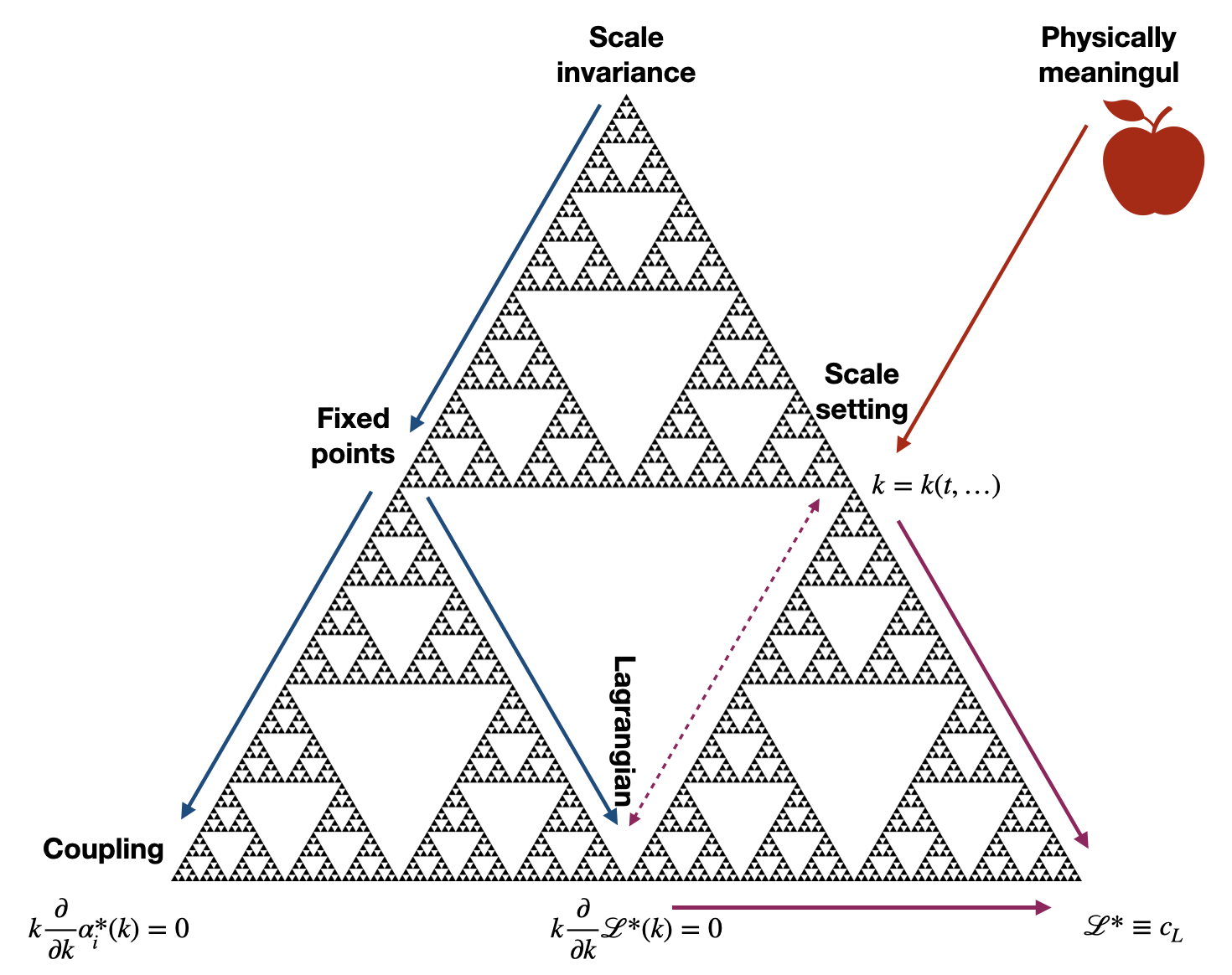
Figure 1: Conceptual map, that shows how SI combined with a physically meaningful prediction motivate ELFP

Imposing both, a Lagrangian independence of $k$ and a e.g. a space-time dependence of $k=k(t)$, we have to demand that the effective Lagrangian is space-time independent. Based on this simple observation, let us hypothesize a different class of idealized regime of SI, which we call the effective Lagrangian fixed point (ELFP):

“The Lagrangian of a theory that has reached an ELFP will remain constant and thus independent of changes in the scale $k$, and after a scale-setting also independent of continuous physical parameters of the system (such as time for the case of cosmology)”

$${\mathcal{L}}={\mathcal{L}}^{*}=c_{L}.$$ (9)

Finally, we note that the hypothesis (9) is specially suitable for a gravitational system, where matter degrees of freedom are negligible. The reason for this is, that the equations of motion for all matter Lagrangian are invariant under a shift ${\mathcal{L}}\rightarrow{\mathcal{L}}+c_{L}$. This invariance gets lost, when the system is coupled to gravity, a fact which lies in the core of the cosmological constant problem Padmanabhan:2006cj .

I.5 Structure of the paper

This work is organized as follows: After this introduction we will present the formalism/method to be used in section II. In section III, we will focus on the cosmological scenario, in particular, in the very early universe, by solving the corresponding scale-dependent Friedman equations with an ELFP. Our results are discussed and summarized in section IV.

II The model

In order to implement and study the above idea of an ELFP, let us consider a concrete model that is close to classical general relativity. A good starting point for this is an Einstein-Hilbert action with cosmological term.

II.1 Scale dependence

In the absence of matter, the leading curvature terms of the gravitational effective action read

$$\Gamma[g_{\mu\nu},k]\equiv\int\mathrm{d}^{4}x\sqrt{-g}{\mathcal{L}}_{k}[g_{\mu\nu}]=\int\mathrm{d}^{4}x\sqrt{-g}\Bigg{[}\frac{1}{2\kappa_{k}}\Bigl{(}R-2\Lambda_{k}\Bigl{)}\Bigg{]},$$ (10)

where $g_{\mu\nu}$ is the metric field, $k$ is the renormalization scale, $\mathcal{L}_{k}$ is the effective Lagrangian density, $g$ is the determinant of the metric field, $R$ is the Ricci scalar, $\Lambda_{k}$ is the cosmological coupling, $\kappa_{k}\equiv 8\pi G_{k}$ is Einstein’s coupling, and $G_{k}$ is the Newton’s coupling. The corresponding equations of motion are Reuter:2004nv ; Reuter:2003ca ; Koch:2010nn ; Domazet:2012tw ; Koch:2014joa ; Contreras:2016mdt

$$G_{\mu\nu}+\Lambda_{k}g_{\mu\nu}=-\Delta t_{\mu\nu}.$$ (11)

The tensor $\Delta t_{\mu\nu}$ encodes the scale–dependence of the gravitational coupling. It is given by

$$\Delta t_{\mu\nu} =G_{k}\Bigl{(}g_{\mu\nu}\square-\nabla_{\mu}\nabla_{\nu}\Bigl{)}G_{k}^{-1}.$$ (12)

Note, that the equations (11) with their local covariant structure also arise from different approaches and formulations such as

• a non-dynamical version of Brans-Dicke theory Brans:1961sx ;

• a particular (minimal) case of the broader class of scalar-tensor theories of gravity Damour:1992kf ; Fujii:2003pa ;

• $f(R)$ gravity Sotiriou:2008rp , if one imposes that $G(k)$ and $\Lambda(k)$ are functions of the Ricci scalar.

II.2 Fixed point condition for the effective Lagrangian

To explore the physics of our hypothetical ELFP we implement it at the level of the action (10) in terms of a Lagrange multiplyer $\lambda$

$$\left.\Gamma\right|_{\mathrm{ELFP}}\left(g_{\mu\nu},k,\lambda\right)\equiv\int\mathrm{d}^{4}x\sqrt{-g}\left({\mathcal{L}}_{k}-\lambda\left({\mathcal{L}}_{k}-c_{L}\right)\right).$$ (13)

This action is manifestly reparametrization invariant. Thus, general covariance of the model is assured. The action (13) can be varied with respect to the three fields $(g_{\mu\nu},\,k,\,\lambda)$, giving three equations of motion. First, one can vary with respect to the auxiliary field $\lambda$ giving the ELFP condition of a constant Lagrangian

$${\mathcal{L}}|_{\mathrm{ELFP}}=c_{L}.$$ (14)

Second, the equation which arises from variations with respect to the scale-field $k$, is

$$\frac{\partial{\mathcal{L}}_{k}}{\partial k}\cdot(1-\lambda)=0.$$ (15)

This equation is trivially solved by (14). The third set of equations arises from variations with respect to the metric field. These equations are identical to (11), with the replacement

$$G_{k}\rightarrow\tilde{G}_{k}\equiv\frac{G_{k}}{1-\lambda}.$$ (16)

In what follows, we will solve the equations for this effective gravitational coupling and drop the “tilde” notation.

III Exploring an ELFP scenario in cosmology

Now, that the stage is set in terms of the action (13), we will explore this model in a cosmological context.

III.1 General considerations

In the very early universe we expect:

• Physics is dominated by higher curvature terms in the gravitational sector. Thus, if this is true, we can neglect the impact of matter contributions $T_{\mu\nu}=0$.

• The Universe is in a quantum regime, which means that scale-dependence in the gravitational couplings is not negligible, in particular: $G=G_{k}$ and $\Lambda=\Lambda_{k}$. Due to limited algebraic and computational power, we restrict to these two couplings in the gravitational sector.

• The Universe is in a extremely symmetric state, which means that the metric is homogeneous and only time dependent, just like the SD couplings

  $$g_{\mu\nu} = g_{\mu\nu}(t),$$ (17)

  $$G_{k} = G(t),$$ (18)

  $$\Lambda_{k} = \Lambda(t).$$ (19)

  Further, and this is crucial, the scale setting is maximally insensitive to the choice of the quantum scale, which is implemented by (14).

There is a remarkable consequence of these conditions and the ELFP relation (14). It allows to solve the equations directly for $G=G(t)$ and $\Lambda=\Lambda(t)$, as it will be shown in the next section.

III.2 Ansatz

The condition of homogeneity is reflected by a line element

$$ds^{2}=-dt^{2}+a^{2}(t)(dx^{2}+dy^{2}+dz^{2}).$$ (20)

For this line element the equations of motion (11) simplify to the SD Friedmann equations

$$\Lambda = -\frac{3\dot{a}(a\dot{G}-G\dot{a})}{a^{2}G},$$ (21)

$$\Lambda-\frac{\dot{a}^{2}}{a^{2}} = \frac{2\dot{a}\dot{G}-2G\ddot{a}}{Ga}+\frac{G\ddot{G}-2\dot{G}^{2}}{G^{2}}$$ (22)

and the ELFP condition

$$\frac{6(\dot{a}^{2}+a\ddot{a})}{a^{2}G}-2\frac{\Lambda(t)}{G(t)}=c_{L}.$$ (23)

One verifies that (21) and (22) simplify to the usual “classical” Friedman equation

$$\frac{\dot{a}^{2}}{a^{2}}=\frac{\Lambda_{0}}{3},$$ (24)

when the couplings become constants $G\rightarrow G_{0}$ and $\Lambda\rightarrow\Lambda_{0}$, which is a solution of (21) -(23) . The “classical” equations (24) are solved by an exponential growth of the scale-factor

$$a_{cl}(t)=a_{0}\exp\left(t\sqrt{\frac{\Lambda_{0}}{3}}\right)\,.$$ (25)

The relations (21), (22) and (23) correspond to a higher-order system, but, as it will be shown, the system can be integrated analytically.

III.3 Solving the equations

For solving, the equations (21, 22, 23), one can start with algebraic identities for $\Lambda$. For example, Eq. (21) can be read as identity for $\Lambda$. Alternatively one can also read $\Lambda$ from Eq. (23) as

$$\Lambda(t)=\frac{6(\dot{a}^{2}+a\ddot{a})}{2a^{2}}-G\frac{c_{L}}{2}.$$ (26)

Even though, the two conditions (21) and (26) do not look identical, their difference must vanish. This difference can be translated into a condition on $\dot{G}$

$$\dot{G}=G\frac{c_{L}aG-6\ddot{a}}{6\dot{a}}.$$ (27)

Deriving the condition (27) with respect to $t$, gives an analogous condition for $\ddot{G}$. Now, one use this on the two conditions and (26) on (21), to get a decoupled differential equation

$$\frac{G^{2}}{\dot{a}}\left(2\dot{a}^{3}-a\dot{a}\ddot{a}-a^{2}\frac{d^{3}a}{dt^{3}}\right)=0.$$ (28)

We can recognize the time derivative of the Ricci scalar in the term between parenthesis,

$$\frac{R(t)}{6}=\frac{\dot{a}^{2}}{a^{2}}+\frac{\ddot{a}}{a},$$ (29)

therefore an important class of solutions of (28), described by $\dot{R}=0$, corresponds to

$$R=c_{R},$$ (30)

where $c_{R}$ is an integration constant.

We will present two alternative complementary ways to express the new solutions. Albeit it could be self-evident, let us reinforce that a concrete form of the scale factor plays a critical role at the moment of identifying the corresponding integration constants. In what follows, we will consider a solution written in terms of exponential functions, trying to mimic the classical scale factor representation. Thus, by replacing Eq. (30) we can find a solution of Eq. (29):

$$a(t) =\frac{1}{\sqrt{2}}c_{2}e^{\frac{t}{2}\sqrt{\frac{c_{R}}{3}}}\sqrt{e^{c_{1}\sqrt{\frac{c_{R}}{3}}}+e^{-(2t+c_{1})\sqrt{\frac{c_{R}}{3}}},}$$ (31)

and, subsequently, we can replace Eq. (31) into Eq. (27) to get a compact expression for the Newton’s coupling, which is

$$G(t) =\frac{c_{R}\sqrt{Y(t)(Y(t)^{2}+1)}}{c_{L}\sqrt{Y(t)}\Bigl{(}\sqrt{Y(t)^{2}+1}-(Y(t)^{2}-1){}_{2}F_{1}\Bigl{(}\frac{1}{4},\frac{1}{2};\frac{5}{4};-Y(t)^{2}\Bigl{)}\Bigl{)}+c_{3}c_{R}(Y(t)^{2}-1)},$$ (32)

where we have defined the auxiliary function $Y(t)$,

$$Y(t)\equiv\exp\left(\sqrt{\frac{c_{R}}{3}}(t+c_{1})\right),$$ (33)

and finally, we use Eq.(26), to obtain the cosmological coupling

$$\Lambda(t) =\frac{1}{2}\Bigl{(}c_{R}-c_{L}G(t)\Bigl{)},$$ (34)

where the gravitational coupling is given in (32). At this point it is clear that a trivial identification of the integration constants is a difficult task, at least in the present representation. However, if we consider the scale factor in terms of hyperbolic functions, we can clearly identify Newton’s constant (at $t=t_{i}$). Inserting (29) in (30) and integrating it yields the solution for the scale factor

$$a(t)=c_{2}\Bigg{(}\cosh{\left[\sqrt{\frac{c_{R}}{3}}\Bigl{(}c_{1}+t\Bigl{)}\right]}\Bigg{)}^{1/2},$$ (35)

where $c_{1,2}$ are the corresponding integration constants. This solution, Eq. (35), can be inserted back into (27) leading to an ordinary differential equation for $G(t)$,

$$\dot{G}(t)=F_{1}(t)G(t)+F_{2}(t)G(t)^{2}\,,$$ (36)

where

$$F_{1}(t)= -\sqrt{c_{R}/3}\mathrm{coth}(\sqrt{c_{R}/3}(t+c_{1}))+\frac{\sqrt{c_{R}/3}}{2}\mathrm{tanh}(\sqrt{c_{R}/3}(t+c_{1}))\,,$$ (37)

$$F_{2}(t)= \frac{c_{L}}{3\sqrt{c_{R}/3}}\mathrm{coth}(\sqrt{c_{R}/3}(t+c_{1}))\,.$$ (38)

The equation has the Bernoulli form and therefore the general solution can be written as

$$\frac{1}{G(t)}=\exp\left(-\int_{t_{i}}^{t}dt^{\prime}F_{1}\right)\left[\frac{1}{G_{i}}-\int_{t_{i}}^{t}dt^{\prime}F_{2}\exp\left(\int_{t_{i}}^{t^{\prime}}dt^{\prime\prime}F_{1}\right)\right]\,,$$ (39)

where $G_{i}$ is an integration constant that has the meaning of the value of $G(t)$ at the time $t_{i}$, $G(t_{i})=G_{i}$. The following expressions are useful:

$$\exp\left(\int_{t_{i}}^{t}dt^{\prime}F_{1}\right)=\frac{\mathcal{F}(t;c_{R},c_{1})}{\mathcal{F}(t_{i};c_{R},c_{1})}\,,$$ (40)

where

$$\mathcal{F}(t;c_{R},c_{1})=\frac{\sqrt{\mathrm{cosh}(\sqrt{c_{R}/3}(t+c_{1}))}}{\mathrm{sinh}(\sqrt{c_{R}/3}(t+c_{1}))}\,,$$ (41)

and

$$\int_{t_{i}}^{t}dt^{\prime}F_{2}\exp\left(\int_{t_{i}}^{t^{\prime}}dt^{\prime\prime}F_{1}\right)= \frac{c_{L}}{|c_{R}|}\left[1-\frac{\mathcal{F}(t;c_{R},c_{1})}{\mathcal{F}(t_{i};c_{R},c_{1})}\right.$$

$$- \left.\frac{i}{\mathcal{F}(t_{i};c_{R},c_{1})}(E^{(F)}(i\sqrt{c_{R}/12}(t+c_{1}),\ 2)\right.$$

$$- \left.E^{(F)}(i\sqrt{c_{R}/12}(t_{i}+c_{1}),\ 2)\right]\,,$$ (42)

where

$$E^{(F)}(x,m)=\int_{0}^{x}d\theta\frac{1}{\sqrt{1-m\sin^{2}\theta}}\,,$$ (43)

is an elliptic function of the first kind. Using (40) and (42) in (39) we get

$$\frac{1}{G(t)}= \frac{\mathcal{F}(t_{i};c_{R},c_{1})}{\mathcal{F}(t;c_{R},c_{1})}\left[\frac{1}{G_{i}}-\frac{c_{L}}{|c_{R}|}+\frac{c_{L}}{|c_{R}|}\frac{\mathcal{F}(t;c_{R},c_{1})}{\mathcal{F}(t_{i};c_{R},c_{1})}\right.$$

$$+ \left.\frac{ic_{L}}{|c_{R}|\mathcal{F}(t_{i};c_{R},c_{1})}(E^{(F)}(i\sqrt{c_{R}/12}(t+c_{1}),\ 2)\right.$$

$$- \left.E^{(F)}(i\sqrt{c_{R}/12}(t_{i}+c_{1}),\ 2))\right]\,.$$ (44)

We will see that the behavior of $G(t)$ depends crucially of the values of $G_{i}$, $c_{L}$ and $c_{R}$.

III.4 Physical interpretation of the integration constants

The above solution has five free parameters which consist of one actual parameter of the Lagrangian $c_{L}$ and four integration constants $c_{R}$, $c_{1}$, $c_{2}$ and $G_{i}$. In this subsection these parameters will be brought into a more intuitive form.

Let’s first study the solution $a(t)$. It is straight forward to see that (35) describes a bouncing scale factor and that $c_{1}$ defines the time of the bounce, thus we write

$$c_{1}=-t_{b}.$$ (45)

The condition

$$\lim_{t_{b}\rightarrow-\infty}a(t)=a_{cl}(t)$$ (46)

allows us to rewrite the two constants $c_{R}$ and $c_{2}$. From the Ricci scalar of the classical solution

$$R|_{a_{cl}}=4\Lambda_{0},$$ (47)

we relabel the corresponding integration constant

$$c_{R}\equiv 4\Lambda_{0}.$$ (48)

Next, fix the constant

$$c_{2}=\sqrt{2}a_{0}\exp{\left(\sqrt{\frac{\Lambda_{0}}{3}}t_{b}\right)}.$$ (49)

After these re-definitions the scale-factor reads in terms of the integration constants $\Lambda_{0},t_{b}$ and $a_{0}$

$$a=\sqrt{2}a_{0}\exp{\left(\sqrt{\frac{\Lambda_{0}}{3}}t_{b}\right)}\left(\cosh{2\sqrt{\frac{\Lambda_{0}}{3}}(t-t_{b})}\right)^{1/2}.$$ (50)

Similarly we can proceed with the gravitational coupling. For this, we keep in mind that there are four time-scales involved in the definition of $G(t)$: $t_{b}<t_{i}<t$.

For large $t$ the gravitational coupling drops to zero, $\lim_{t\rightarrow\infty}G(t)=0$, see figures (4,5). However, for a short period of time, $G(t)$ has a plateau behavior. The time length of the plateau depends on the parameters, as we see it in the figure. There is an special case in which the time length of the plateau get enhanced and it occurs when $c_{L}=2\Lambda_{0}/G_{i}$. To get a better understanding of this behavior, we explore the regime $t_{b}\ll t_{i},t$, where we can approximate the functions (37, 37)

$$F_{1}|_{t_{b}\ll t_{i}} = -\sqrt{\frac{\Lambda_{0}}{3}}$$ (51)

$$F_{2}|_{t_{b}\ll t_{i}} = \frac{c_{L}}{2\sqrt{3\Lambda_{0}}}.$$ (52)

In this regime the differential equation (36) reads

$$\frac{d}{dt}\left(\frac{1}{G}\right)=-\sqrt{\frac{\Lambda_{0}}{3}}\left(\frac{1}{G}\right)-\frac{c_{L}}{2\sqrt{3\Lambda_{0}}}.$$ (53)

We can solve this linear differential equation with the initial condition $G(t_{i})=G_{i}$, giving

$$\left(\frac{1}{G}\right)=\exp\left(\Delta t\sqrt{\frac{\Lambda_{0}}{3}}\right)\left(\frac{1}{G_{i}}-\frac{c_{L}}{2\Lambda_{0}}\right)+\frac{c_{L}}{2\Lambda_{0}},$$ (54)

where $\Delta t\equiv t-t_{i}\gg t_{b}$. There are two main cases, firstly if $c_{L}\neq 2\Lambda_{0}/G_{i}$, then:

$$\lim_{\Delta t\rightarrow 0}G(t)=G_{i}\,,\quad\lim_{\Delta t\rightarrow 0}\Lambda(t)=2\Lambda_{0}-\frac{c_{L}G_{i}}{2}\\$$ (55)

and the solution has the following asymptotic behavior

$$\lim_{\Delta t\rightarrow\infty}G(t)=0\,,\quad\lim_{\Delta t\rightarrow\infty}\Lambda(t)=2\Lambda_{0}\,.\\$$ (56)

Also, if $G_{i}<2\Lambda_{0}/c_{L}$, then $G(t)$ continuously but quickly decrease to a vanishing value (figure 4). If $G_{i}>2\Lambda_{0}/c_{L}$, then $G(t)$ may blow up very quickly to then emerge from $-\infty$ and approach a vanishing value very quickly (figure 5) Secondly, in the fine-tuned case, $c_{L}=2\Lambda_{0}/G_{i}$, we have a regime where both couplings appear to be approximately constant

$$G(t)=\frac{2\Lambda_{0}}{c_{L}}\,,\quad\Lambda(t)=\Lambda_{0}\,.$$ (57)

This case is special because the time duration of the plateau of $G(t)$ gets enhanced. We denote the time length at which $G(t)$ is approximately constant by $\Delta t_{d}$. We found it being proportional to

$$\Delta t_{d}\sim\frac{1}{\sqrt{c_{L}}}=\sqrt{\frac{G_{i}}{2\Lambda_{0}}}\,.$$ (58)

We determined by a numerical analysis by looking at the time at which $G(t)=(1/2)G_{i}$. In figure 6, we vary $\Lambda_{0}$ and we can observe that a smaller $\Lambda_{0}$ implies a later drop of the gravitational coupling.

To summarize this section, an intuitive parametrization of our four integration constants can be given in terms of the scale factor normalization at late times $a_{0}$, the expansion factor at late times $\Lambda_{0}$, the bouncing time $t_{b}$, and the value of the gravitational coupling at an intermediate time $G(t_{i})=G_{i}$. For this scenario the couplings approach the values given in (56). If further, $G_{i}=\frac{2\Lambda_{0}}{c_{L}}$ and we take the singular limit $t_{i}\rightarrow\infty$ with $t_{i}\gg t_{b}$, the couplings approach finite constant values (57).

III.5 Curvature invariants

One can further study the curvature invariants of our solution. The Ricci scalar takes the same value as in the classical case, $R=4\Lambda_{0}$, however higher curvature scalars like the Kretschmann scalar are sensitive to the deviations from the classical case:

$$R^{\mu\nu\alpha\beta}R_{\mu\nu\alpha\beta}=\frac{8}{3}\Lambda_{0}^{2}\left(1+\text{sech}\left(2\sqrt{\frac{\Lambda_{0}}{3}}(t-t_{b})\right)\right).$$ (59)

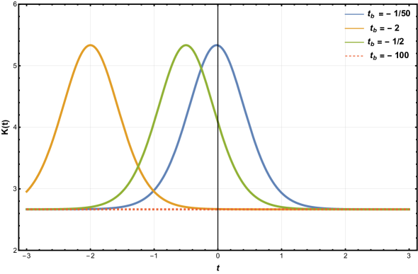
Figure 2: Visualization of the Kretschmann scalar in Eq. (59) for four different choices of the bouncing time $t_{b}$. In all the scenarios, $\Lambda_{0}$ is set to one.

In figure 2, we observe two interesting features. First, one immediately notices that as the bouncing time is pushed back in time, the contribution from the second term in Eq. (59) becomes negligible for late times and the solution converges to the classical case as we have highlighted this in the figure with dashed line. Second, when time $t$ reaches the bouncing time $t_{b}$, the argument in the hyperbolic function becomes zero and we have a maximum and again, as $t$ moves forward or backwards away from $t_{b}$, we recover the classical Kretschmann scalar. In terms of the statefinder parameters the model is described by a straight line in the $(q,r)$-plane with slope unity that finishes in the classical point $(q,r)_{\mathrm{cl}}=(1,1)$

IV Discussion

In this final section, we revisit and discuss the preceding results.

IV.1 The dynamical variables

Our results provide several interesting features for the functions $a(t),\,G(t),\,\Lambda(t)$. Since analytical structure of $G(t)$ is more involved than the structure of the other functions, the discussion of $G(t)$ will require somewhat more space than the discussion of the other two functions.

• $a(t)$: In the scale factor we notice truly remarkable features that can be read from the figure 3. We realize at large times the function $a(t)$ shows the expected classical exponential evolution. However, when evolving backwards in time, the curve flattens, reaches a minimum and then grows again. We observe that, for sufficiently large times the solution becomes harder to distinguish from a purely classical one.

  

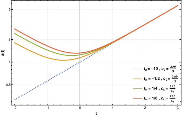
  Figure 3: Visualization of the evolution of the scale factor for four different scenarios all with $c_{L}=2\Lambda_{0}/G_{i}$. The y-axis is in logarithmic scale. Both $\Lambda_{0}$ and $G_{i}$ are set to one in all the four scenarios.

• $G(t)$: The time dependence of the gravitational coupling is shown in figures (4,5). In the figure, we have defined three different categories by keeping the ratio $2\Lambda_{0}/G_{i}$ and defining $c_{L}$ to be equal, greater and smaller than $2\Lambda_{0}/G_{i}$. We notice some features from the behaviour of the coupling. First, the coupling drops to zero at very large times and this behaviour is unavoidable. However, as mentioned in section III.3, by fine-tuning the solution of $G(t)$, it is possible to keep the coupling constant for some time before it drops to zero. This can be seen from the scenarios in the middle column of the figure. We also notice that in all scenarios the coupling diverges as the time $t$ approaches the bouncing time $t_{b}$. The reason for this is that the function $\mathcal{F}(t,c_{R},t_{b})=\frac{\sqrt{\text{cosh}(\sqrt{cR/3}(t-tb)}}{\text{sinh}(\sqrt{cR/3}(t-tb)}$ diverges, causing the coupling $G(t)$ to diverge as well.
  Also, as discussed in section III.4, for late times and when $t_{b}\ll t,t_{i}$, one can use approximations to understand why the couplings become approximately constant. However, one needs to be careful with this approximation. In order to use this asymptotic feature of the model, the approximation has to be made at the level of the differential equations as discussed. Once the full differential equations, without the approximations in section III.4, are solved and the solution (Eq. 44) is found, the coupling necessarily drops to zero at some late enough time.
  

  

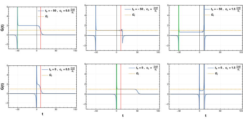
  Figure 4: Visualization of the evolution of the scale-dependent gravitational coupling constant for different scenarios with $t_{b}<t_{i}$ . In the matrix, the rows correspond to the variation of the bouncing time $t_{b}$ and the columns correspond to the three different cases $c_{L}<2\Lambda_{0}/G_{i}$, $c_{L}=2\Lambda_{0}/G_{i}$ and $c_{L}>2\Lambda_{0}/G_{i}$, respectively. The vertical green line indicates the chosen bouncing time and the vertical red line indicates the chosen initial time where the value of $G_{i}$ is fixed. In all the figures, $G_{i}$ and $\Lambda_{0}$ are set to one.

  

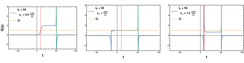
  Figure 5: Same as Figure 4 but with $t_{b}>t_{i}$.

  

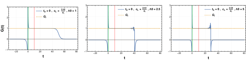
  Figure 6: Visualization of $G(t)$ in the case where $\Lambda_{0}$ is being varied, illustrating the fact that a smaller $\Lambda_{0}$ makes $G(t)$ non-zero for a larger period of time. $G_{i}$ and $t_{i}$ are set to 1 and 10, respectively.

  One notes further that for $c_{L}=0$ the analytical form of $G(t)$ gets particularly simple, but apart from this, the qualitative behaviour remains the same.

• $\Lambda(t)$: The evolution of the cosmological term is shown in figure 7. In the evolution backwards and also forwards in time one notes that the cosmological term reaches a constant value of $2\Lambda_{0}$ due to the behaviour our of the scale dependent coupling $G(t)$. Also, due to the behaviour of $G(t)$, when $G(t)$ diverges, so does $\Lambda(t)$ but with a different sign because of the minus sign in Eq. (34).

  

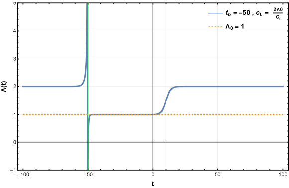
  Figure 7: Visualization of the evolution of the scale-dependent cosmological constant for a scenario with $c_{L}=2\Lambda_{0}/G_{i}$. The vertical green line corresponds to the bouncing time and the vertical red line corresponds to the initial time where the value of $G_{i}$ is being fixed. The values of $G_{i}$ and $\Lambda_{0}$ are set to one.

IV.2 Towards a dynamical systems perspective

Attractors are fundamental concepts in the study of dynamical systems. An attractor is a set or a point towards which a dynamical system evolves over time, regardless of the starting conditions (within a given region). Attractors represent the long-term behavior of systems. There are various types of attractors, and they can be distinguished based on their structure and the nature of the dynamical system: Fixed points, attractors, limit cycles, limit torus, strange attractors.

It is interesting to analyze the above results from the perspective of such a dynamical system. The dynamical variables are $a(t)$ and $G(t)$. They span the four dimensional phase space ${\bf{X}}\equiv\left\{a,\,\dot{a},G,\,\dot{G}\right\}(t)$. Analyzing the time evolution of our solution we find that

$${\bf{X}}_{FP1}=\left\{a_{cl},\,\dot{a}_{cl},0,\,0\right\}(t\rightarrow\infty)$$ (60)

is a stable fixed point (attractor) of the dynamical system. There further seems to be another, unstable fixed point

$${\bf{X}}_{FP2}=\left\{a_{cl},\,\dot{a}_{cl},\frac{2\Lambda_{0}}{c_{L}},\,0\right\}(t\gg t_{b}).$$ (61)

Here, it is important to note that a priory fixed points of RG systems are not related to fixed points of dynamical systems, because the latter are understood as characteristics of the time evolution of a system like $\left\{a,\,\dot{a},G,\,\dot{G}\right\}(t)$, while the former are related to scale transformations of a different system $\Gamma(k,\dots)$. This clear separation of the two concepts gets however bridged as soon as one seeks a physical interpretation of the RG system in terms of a scale setting (8) as discussed in section I.3. It is highly intriguing to observe that demanding an ELFP for an effective action leads to a dynamical system which has one attractive and one repulsive fixed point.

It will be an interesting subject of future studies, to explore this apparent scale-setting induced link between RG fixed points and the attractors of the corresponding dynamical systems. In particular since such attractors have also been found in the broader context of certain tensor-scalar theories Damour:1992kf .

IV.3 Parallels to bouncing cosmology models

Bouncing cosmologies refer to models of the universe in which there was a contraction phase that preceded the current expansion phase, and instead of a singularity (as in the Big Bang model), there was a “bounce” at some minimum scale. Essentially, these models propose that our universe underwent a contraction, reached a small but finite size, and then began expanding, which is the phase we observe today. They are interesting because they can serve for avoiding singularities, provide an alternative to inflation, shed light on quantum gravity, provide cyclic universes, and at timed provide observational clues.

The results presented above show intriguing similarities with completely different approaches to gravity which also produce such a bouncing cosmology. These are for example, Horava-Lifshitz gravity  Horava:2009uw ; Horava:2009if , $f(R)$ gravity 10.1093/mnras/150.1.1 ; Nojiri:2009kx , $f({\mathcal{G}})$ gravity Astashenok:2015haa , $f(T)$ gravity Geng:2011aj ; Maluf:2013gaa and even loop quantum cosmology Finelli:2001sr ; Laguna:2006wr ; Corichi:2007am ; Bojowald:2008pu (for a summary see Nojiri:2017ncd ). Since the ELFP was proposed from a perspective of scale invariance, it is interesting that the bounce we find seems to reflect the essence of another cosmological model, whose construction principle is conformal symmetry Gurzadyan:2013cna . I is interesting to carry out a detailed comparison between the $f(R)$ models with bounce and our ELFT proposal, which could be further explored in future studies.

V Summary and conclusions

In this paper, we have defined and motivated the notion of an effective Lagrangian fixed point. Based on the hypothesis that such a fixed point exists in some regime of a scale-dependent theory gravitational theory, we formulated a model that implements such a ELFP in the low curvature expansion (13). Then we solved and analyzed the resulting field equations for a cosmology (20). The solution has four integration constants $\Lambda_{0},a_{0},G_{i},t_{b}$ and one parameter $c_{L}$, which we treat as the five-dimensional parameter space. We explored the solution of our model in terms of this parameter space by studying the time behaviour of the gravitational coupling, curvature invariants, and the scale factor. For the gravitational coupling $G(t)$ we find that for $t>t_{b,i}$, the evolution is continuous and converging asymptotically to zero. There is, however, a notable case on a four-dimensional subspace such that $c_{L}=2\Lambda_{0}/G_{i}$, where the gravitational coupling enters a regime of “meta-stability” that delays its otherwise rapid fall to zero. For the scale factor and the derived Kretschmann scalar we observe remarkable features. The parameter space contains a distinguished time $t_{b}$, which can be identified as bouncing time. At this time our model predicts a bounce, avoiding a singular behaviour at the “origin”. Interestingly, at later times $t\gg t_{b}$, the scale factor and the curvature invariants behave just as if it was goverened by the classical Einstein equations with a cosmological constant and a constant gravitational coupling, even though the couplings are not constant and eventually not even finite.

Thus, the ELFP cosmological model has highly non trivial evolution of its couplings, but it reproduces the exponential expansion for sufficiently large times, while it provides a “save bounce” at earlier times.

Acknowlegements

This work has been partially funded by Agencia Nacional de Investigación y Desarrollo (ANID) through FONDECYT grant 1230112. A.R. is funded by the Generalitat Valenciana (Prometeo excellence programme grant CIPROM/2022/13) and by the Maria Zambrano contract ZAMBRANO 21-25 (Spain).

References

- (1) Steven Weinberg. Critical Phenomena for Field Theorists. In 14th International School of Subnuclear Physics: Understanding the Fundamental Constitutents of Matter, 8 1976.
- (2) Christof Wetterich. Exact evolution equation for the effective potential. Phys. Lett. B, 301:90–94, 1993.
- (3) Tim R. Morris. The Exact renormalization group and approximate solutions. Int. J. Mod. Phys. A, 9:2411–2450, 1994.
- (4) Alfio Bonanno and Martin Reuter. Renormalization group improved black hole space-times. Phys. Rev. D, 62:043008, 2000.
- (5) M. Reuter and Frank Saueressig. Renormalization group flow of quantum gravity in the Einstein-Hilbert truncation. Phys. Rev. D, 65:065016, 2002.
- (6) Daniel F. Litim and Jan M. Pawlowski. Completeness and consistency of renormalisation group flows. Phys. Rev. D, 66:025030, 2002.
- (7) M. Reuter and H. Weyer. Running Newton constant, improved gravitational actions, and galaxy rotation curves. Phys. Rev. D, 70:124028, 2004.
- (8) A. Bonanno and M. Reuter. Spacetime structure of an evaporating black hole in quantum gravity. Phys. Rev. D, 73:083005, 2006.
- (9) M. Niedermaier. The Asymptotic safety scenario in quantum gravity: An Introduction. Class. Quant. Grav., 24:R171–230, 2007.
- (10) Roberto Percacci. Asymptotic Safety. pages 111–128, 9 2007.
- (11) N. Dupuis, L. Canet, A. Eichhorn, W. Metzner, J. M. Pawlowski, M. Tissier, and N. Wschebor. The nonperturbative functional renormalization group and its applications. Phys. Rept., 910:1–114, 2021.
- (12) Akihiro Ishibashi, Nobuyoshi Ohta, and Daiki Yamaguchi. Quantum improved charged black holes. Phys. Rev. D, 104(6):066016, 2021.
- (13) Jose Miguel Ladino, Carlos A. Benavides-Gallego, Eduard Larrañaga, Javlon Rayimbaev, and Farrux Abdulxamidov. Charged spinning and magnetized test particles orbiting quantum improved charged black holes. Eur. Phys. J. C, 83(11):989, 2023.
- (14) R. Torres. Non-singular quantum improved rotating black holes and their maximal extension. Gen. Rel. Grav., 49(6):74, 2017.
- (15) Jose Miguel Ladino and Eduard Larrañaga. Motion of a spinning particle around an improved rotating black hole. Int. J. Mod. Phys. D, 31(12):2250091, 2022.
- (16) Ángel Rincón and Grigoris Panotopoulos. Quasinormal modes of an improved Schwarzschild black hole. Phys. Dark Univ., 30:100639, 2020.
- (17) Joan Sola. Cosmological constant and vacuum energy: old and new ideas. J. Phys. Conf. Ser., 453:012015, 2013.
- (18) Ilya L. Shapiro, Joan Sola, Cristina Espana-Bonet, and Pilar Ruiz-Lapuente. Variable cosmological constant as a Planck scale effect. Phys. Lett. B, 574:149–155, 2003.
- (19) Joan Sola and Hrvoje Stefancic. Effective equation of state for dark energy: Mimicking quintessence and phantom energy through a variable lambda. Phys. Lett. B, 624:147–157, 2005.
- (20) Cristina Espana-Bonet, Pilar Ruiz-Lapuente, Ilya L. Shapiro, and Joan Sola. Testing the running of the cosmological constant with type Ia supernovae at high z. JCAP, 02:006, 2004.
- (21) Javier Grande, Joan Sola, Spyros Basilakos, and Manolis Plionis. Hubble expansion and structure formation in the ’running FLRW model’ of the cosmic evolution. JCAP, 08:007, 2011.
- (22) Norman Cruz, Gabriel Gomez, Esteban Gonzalez, Guillermo Palma, and Angel Rincon. Exploring models of running vacuum energy with viscous dark matter from a dynamical system perspective. Phys. Dark Univ., 42:101351, 2023.
- (23) Grigoris Panotopoulos, Ángel Rincón, Giovanni Otalora, and Nelson Videla. Dynamical systems methods and statender diagnostic of interacting vacuum energy models. Eur. Phys. J. C, 80(3):286, 2020.
- (24) Benjamin Koch, Ignacio A. Reyes, and Ángel Rincón. A scale dependent black hole in three-dimensional space–time. Class. Quant. Grav., 33(22):225010, 2016.
- (25) Ángel Rincón and Benjamin Koch. Scale-dependent rotating BTZ black hole. Eur. Phys. J. C, 78(12):1022, 2018.
- (26) Ángel Rincón and Grigoris Panotopoulos. Quasinormal modes of scale dependent black holes in ( 1+2 )-dimensional Einstein-power-Maxwell theory. Phys. Rev. D, 97(2):024027, 2018.
- (27) Ángel Rincón, Ernesto Contreras, Pedro Bargueño, Benjamin Koch, Grigorios Panotopoulos, and Alejandro Hernández-Arboleda. Scale dependent three-dimensional charged black holes in linear and non-linear electrodynamics. Eur. Phys. J. C, 77(7):494, 2017.
- (28) Ernesto Contreras, Ángel Rincón, Grigoris Panotopoulos, Pedro Bargueño, and Benjamin Koch. Black hole shadow of a rotating scale–dependent black hole. Phys. Rev. D, 101(6):064053, 2020.
- (29) Christof Wetterich. Effective average action in statistical physics and quantum field theory. Int. J. Mod. Phys. A, 16:1951–1982, 2001.
- (30) I. L. Buchbinder, S. D. Odintsov, and I. L. Shapiro. Effective action in quantum gravity. 1992.
- (31) Dario Benedetti, Pedro F. Machado, and Frank Saueressig. Asymptotic safety in higher-derivative gravity. Mod. Phys. Lett. A, 24:2233–2241, 2009.
- (32) Alessandro Codello, Roberto Percacci, and Christoph Rahmede. Investigating the Ultraviolet Properties of Gravity with a Wilsonian Renormalization Group Equation. Annals Phys., 324:414–469, 2009.
- (33) Ivan Donkin and Jan M. Pawlowski. The phase diagram of quantum gravity from diffeomorphism-invariant RG-flows. 3 2012.
- (34) O. Lauscher and M. Reuter. Ultraviolet fixed point and generalized flow equation of quantum gravity. Phys. Rev. D, 65:025013, 2002.
- (35) M. Reuter. Nonperturbative evolution equation for quantum gravity. Phys. Rev. D, 57:971–985, 1998.
- (36) Max Niedermaier and Martin Reuter. The Asymptotic Safety Scenario in Quantum Gravity. Living Rev. Rel., 9:5–173, 2006.
- (37) Leonardo Modesto and Lesław Rachwał. Nonlocal quantum gravity: A review. Int. J. Mod. Phys. D, 26(11):1730020, 2017.
- (38) Leonardo Modesto, Lesław Rachwał, and Ilya L. Shapiro. Renormalization group in super-renormalizable quantum gravity. Eur. Phys. J. C, 78(7):555, 2018.
- (39) Xavier Calmet. Vanishing of Quantum Gravitational Corrections to Vacuum Solutions of General Relativity at Second Order in Curvature. Phys. Lett. B, 787:36–38, 2018.
- (40) Mathijs Fraaije, Alessia Platania, and Frank Saueressig. On the reconstruction problem in quantum gravity. Phys. Lett. B, 834:137399, 2022.
- (41) Joan Sola, Adria Gomez-Valent, and Javier de Cruz Pérez. Hints of dynamical vacuum energy in the expanding Universe. Astrophys. J. Lett., 811:L14, 2015.
- (42) Joan Solà, Adrià Gómez-Valent, and Javier de Cruz Pérez. The tension in light of vacuum dynamics in the Universe. Phys. Lett. B, 774:317–324, 2017.
- (43) Ramon Torres. Nonsingular black holes, the cosmological constant, and asymptotic safety. Phys. Rev. D, 95(12):124004, 2017.
- (44) Carlos M. Sendra. Regular scale-dependent black holes as gravitational lenses. Gen. Rel. Grav., 51(7):83, 2019.
- (45) Frank Saueressig, Natalia Alkofer, Giulio D’Odorico, and Francesca Vidotto. Black holes in Asymptotically Safe Gravity. PoS, FFP14:174, 2016.
- (46) Benjamin Koch and Frank Saueressig. Black holes within Asymptotic Safety. Int. J. Mod. Phys. A, 29(8):1430011, 2014.
- (47) Kevin Falls and Daniel F. Litim. Black hole thermodynamics under the microscope. Phys. Rev. D, 89:084002, 2014.
- (48) Benjamin Koch, Carlos Contreras, Paola Rioseco, and Frank Saueressig. Black holes and running couplings: A comparison of two complementary approaches. Springer Proc. Phys., 170:263–269, 2016.
- (49) A. Bonanno and M. Reuter. Cosmology of the Planck era from a renormalization group for quantum gravity. Phys. Rev. D, 65:043508, 2002.
- (50) Martin Reuter and Jan-Markus Schwindt. Scale-dependent metric and causal structures in Quantum Einstein Gravity. JHEP, 01:049, 2007.
- (51) Benjamin Koch and Israel Ramirez. Exact renormalization group with optimal scale and its application to cosmology. Class. Quant. Grav., 28:055008, 2011.
- (52) Silvije Domazet and Hrvoje Stefancic. Renormalization group scale-setting from the action - a road to modified gravity theories. Class. Quant. Grav., 29:235005, 2012.
- (53) Benjamin Koch, Paola Rioseco, and Carlos Contreras. Scale Setting for Self-consistent Backgrounds. Phys. Rev. D, 91(2):025009, 2015.
- (54) Benjamin Koch and C. Laporte. Variational technique for gauge boson masses. Phys. Rev. D, 103(4):045011, 2021.
- (55) Benjamin Koch, Christian Käding, Mario Pitschmann, and René Sedmik. Vacuum energy, the Casimir effect, and Newton’s non-constant. 11 2022.
- (56) Alessia Platania. Dynamical renormalization of black-hole spacetimes. Eur. Phys. J. C, 79(6):470, 2019.
- (57) Astrid Eichhorn and Aaron Held. Image features of spinning regular black holes based on a locality principle. Eur. Phys. J. C, 81(10):933, 2021.
- (58) Astrid Eichhorn and Aaron Held. From a locality-principle for new physics to image features of regular spinning black holes with disks. JCAP, 05:073, 2021.
- (59) Aaron Held. Invariant Renormalization-Group improvement. 5 2021.
- (60) Angel Rincon and Benjamin Koch. On the null energy condition in scale dependent frameworks with spherical symmetry. J. Phys. Conf. Ser., 1043(1):012015, 2018.
- (61) Felipe Canales, Benjamin Koch, Cristobal Laporte, and Angel Rincon. Cosmological constant problem: deflation during inflation. JCAP, 01:021, 2020.
- (62) Pedro D. Alvarez, Benjamin Koch, Cristobal Laporte, and Ángel Rincón. Can scale-dependent cosmology alleviate the tension? JCAP, 06:019, 2021.
- (63) Pedro D. Alvarez, Benjamin Koch, Cristobal Laporte, Felipe Canales, and Angel Rincon. Statefinder analysis of scale-dependent cosmology. JCAP, 10:071, 2022.
- (64) Pedro D. Alvarez, Benjamin Koch, Cristobal Laporte, and Angel Rincon. Cosmological constraints on scale-dependent cosmology. 10 2022.
- (65) M. Reuter and H. Weyer. Renormalization group improved gravitational actions: A Brans-Dicke approach. Phys. Rev. D, 69:104022, 2004.
- (66) Alfio Bonanno, Georgios Kofinas, and Vasilios Zarikas. Effective field equations and scale-dependent couplings in gravity. Phys. Rev. D, 103(10):104025, 2021.
- (67) Benjamin Koch and Frank Saueressig. Structural aspects of asymptotically safe black holes. Class. Quant. Grav., 31:015006, 2014.
- (68) Alfio Bonanno, Benjamin Koch, and Alessia Platania. Gravitational collapse in Quantum Einstein Gravity. Found. Phys., 48(10):1393–1406, 2018.
- (69) Jan M. Pawlowski and Dennis Stock. Quantum-improved Schwarzschild-(A)dS and Kerr-(A)dS spacetimes. Phys. Rev. D, 98(10):106008, 2018.
- (70) John F. Donoghue. A Critique of the Asymptotic Safety Program. Front. in Phys., 8:56, 2020.
- (71) T. Padmanabhan. Why Does Gravity Ignore the Vacuum Energy? Int. J. Mod. Phys. D, 15:2029–2058, 2006.
- (72) Carlos Contreras, Benjamin Koch, and Paola Rioseco. Setting the Renormalization Scale in QFT. J. Phys. Conf. Ser., 720(1):012020, 2016.
- (73) C. Brans and R. H. Dicke. Mach’s principle and a relativistic theory of gravitation. Phys. Rev., 124:925–935, 1961.
- (74) Thibault Damour and Kenneth Nordtvedt. General relativity as a cosmological attractor of tensor scalar theories. Phys. Rev. Lett., 70:2217–2219, 1993.
- (75) Y. Fujii and K. Maeda. The scalar-tensor theory of gravitation. Cambridge Monographs on Mathematical Physics. Cambridge University Press, 7 2007.
- (76) Thomas P. Sotiriou and Valerio Faraoni. f(R) Theories Of Gravity. Rev. Mod. Phys., 82:451–497, 2010.
- (77) Petr Horava. Quantum Gravity at a Lifshitz Point. Phys. Rev. D, 79:084008, 2009.
- (78) Petr Horava. Spectral Dimension of the Universe in Quantum Gravity at a Lifshitz Point. Phys. Rev. Lett., 102:161301, 2009.
- (79) H. A. Buchdahl. Non-Linear Lagrangians and Cosmological Theory. Monthly Notices of the Royal Astronomical Society, 150(1):1–8, 09 1970.
- (80) Shin’ichi Nojiri, Sergei D. Odintsov, and Diego Saez-Gomez. Cosmological reconstruction of realistic modified F(R) gravities. Phys. Lett. B, 681:74–80, 2009.
- (81) Artyom V. Astashenok, Sergei D. Odintsov, and V. K. Oikonomou. Modified Gauss–Bonnet gravity with the Lagrange multiplier constraint as mimetic theory. Class. Quant. Grav., 32(18):185007, 2015.
- (82) Chao-Qiang Geng, Chung-Chi Lee, Emmanuel N. Saridakis, and Yi-Peng Wu. “Teleparallel” dark energy. Phys. Lett. B, 704:384–387, 2011.
- (83) J. W. Maluf. The teleparallel equivalent of general relativity. Annalen Phys., 525:339–357, 2013.
- (84) Fabio Finelli and Robert Brandenberger. On the generation of a scale invariant spectrum of adiabatic fluctuations in cosmological models with a contracting phase. Phys. Rev. D, 65:103522, 2002.
- (85) Pablo Laguna. Numerical Analysis of the Big Bounce in Loop Quantum Cosmology. Phys. Rev. D, 75:024033, 2007.
- (86) Alejandro Corichi and Parampreet Singh. Quantum bounce and cosmic recall. Phys. Rev. Lett., 100:161302, 2008.
- (87) Martin Bojowald. Quantum nature of cosmological bounces. Gen. Rel. Grav., 40:2659–2683, 2008.
- (88) S. Nojiri, S. D. Odintsov, and V. K. Oikonomou. Modified Gravity Theories on a Nutshell: Inflation, Bounce and Late-time Evolution. Phys. Rept., 692:1–104, 2017.
- (89) V. G. Gurzadyan and R. Penrose. On CCC-predicted concentric low-variance circles in the CMB sky. Eur. Phys. J. Plus, 128:22, 2013.