Seismic monitoring of water volume in a porous storage: A field-data study

Abstract

With global groundwater levels undergoing rapid declines, there is an urgent need for advanced methodologies to monitor and manage aquifers. This paper explores the potential of seismic data as a tool for these purposes. Building upon prior studies employing synthetic data, our investigation progresses to analyzing measured data acquired from a field site in Laukaa, Finland. Utilizing neural networks, we directly recover water volume from seismic data, eliminating the need for independent determinations of geometry and porosity. The study involves simulating wave propagation through a coupled poroviscoelastic-viscoelastic medium, employing a three-dimensional discontinuous Galerkin method coupled with an Adams-Bashforth time-stepping scheme. The proposed approach is tested on both field measurements from the Laukaa site and synthetic data, aiming to enhance methodologies for precisely mapping water volume and providing invaluable insights for the development of sustainable water management strategies.

1 Introduction

Groundwater aquifers are facing unprecedented threats, with levels decreasing at alarming rates, often more than one meter per year in many parts of the world. As a result, surface water flows that were previously sustained by groundwater are becoming seasonal or disappearing completely [9]. To ensure sustainable water extraction, it is crucial to have a better understanding of the location and extent of groundwater resources. To tackle these challenges and better understand groundwater resources, this paper explores the application of geophysical seismic data analysis, enhanced by neural network techniques, in monitoring and managing groundwater resources.

Geophysical methods, including seismic techniques, are commonly used tools in the early stages of groundwater exploration and for ensuring sustainable extraction strategies. They offer a cost-effective alternative to drilling, providing laterally continuous data across vast areas, by utilizing variations in seismic velocity and density to detect subsurface features. Seismic methods, in particular, are well-suited for locating and monitoring groundwaters due to the higher seismic velocities exhibited by saturated materials compared to unsaturated ones [11]. The high resolution of seismic methods, both horizontally and vertically, enables the creation of detailed subsurface feature mapping.

This study builds upon the works [14] and [12], in which synthetic seismic data were used to develop computational methodologies for monitoring the water volume of aquifer. The results demonstrated that, by incorporating advanced neural network algorithms, seismic data could provide valuable information about groundwater resources and can be crucial in developing more accurate and efficient models for subsurface water distribution. The current study focuses on utilizing real seismic data to further test and refine these methodologies. By analyzing data from a field site, our objective is to provide more accurate and detailed information about the distribution and extraction of groundwater resources.

In this study, our objective is to explore the estimation of water volume from seismic data obtained in an artificial porous sand-pool located at Laukaa, Finland. In the studied approach, neural networks are employed to directly recover water volume from seismic data, eliminating the necessity for independent determination of geometry and porosity. The seismic data, generated by a drop-weight seismic source, were collected in several acquisition campaigns, following a change in the water table level of the sand pool.

One crucial step involves simulating wave propagation for the training phase of the neural network. The wave propagation simulation involves formulating the governing equations using the coupled viscoelastic and Biot’s poroviscoelastic wave equations [5]. For numerical approximation, we employ the nodal discontinuous Galerkin method formulated in three dimensions [10] coupled with an Adams-Bashforth time-stepping scheme [8]. The applied wave solver builds upon the works presented in references [7] and [12].

In our analysis of neural network-based estimates, we augment our approach by applying the Shapley additive explanation (SHAP) framework [15]. Employing the SHAP framework provides us with a deeper understanding of the estimation process at the receiver level. In our specific context, we focus on understanding the contribution of receivers to our results, rather than aiming to optimize the configuration of the receiver array.

We present a comprehensive study on employing neural networks to characterize water storage using seismic data from the Laukaa test site. Section 2 explores the field measurements at the Laukaa site. In Section 3, we discuss the simulation of measurement data and the synthetic modeling of the site. The use of neural networks to characterize water storage is discussed in Section 4. Section 5 offers a thorough analysis of the results, with a focus on the water volume predictions and the results of the SHAP analysis. In Section 6, we summarize our findings and suggest possible directions for future research.

2 Laukaa test site - field measurements

2.1 Description of the Laukaa test site

The field measurements are conducted in a man-made sand pool located at Natural Resources Institute Finland (Luke) premises in Laukaa, Finland. Generally, sand pool serves a controlled environment to explore groundwater distribution with a knowledge of the media’s geometry and physical parameters. The Laukaa test site stands as a homogeneous and isotropic custom pool, integrated into a recirculating aquaculture system. It contains uniform sand grain size and is surrounded by an impermeable clay lining, as detailed in [17]. The pool’s dimensions are well-defined, facilitating adjustments to the groundwater table level as required. With this setup, it is possible to calculate the actual volumes of water as well as collect the seismic data that corresponds to them.

2.2 Seismic measurements

The seismic measurements were conducted in Laukaa in June 2022. The measurements from the gauge shallow wells were collected to get the ground truth values to calculate the water volume. To study different water levels, we opened a valve to reduce the water table level, followed by a period of stabilization. The stabilization process was monitored by measuring the water table levels from different wells placed along the groundwater flow path.

In our experiments, a metallic rod weight was dropped on a steel plate and served as a source of seismic waves, with an electric brake mechanism to control the rod’s release and prevent multiple hits. The experiments involved shots at 13 specific locations and were conducted at three different drop heights ($\rm{dh}$), consisting of 5, 10, and 15 cm elevations.

For data acquisition, three-component (3C) 5 Hz geophones connected to commercially available 24-bit nodal seismic recorders were used to collect the data. The recorders were deployed along 4 receiver lines (14 per line) with 0.5 m inline and 1.5 m crossline spacing, plus an extra receiver randomly positioned, making a rather fine-scale 3D seismic setup. The recorded time length was 3 seconds with 4 kHz sampling rate.

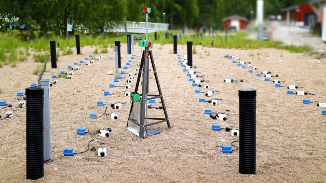
Figure 1: Photo of experimental setup at Laukaa test site, showing the grid of geophones, weight-drop source, and wells to measure the water table level.

Various sources of noise were active throughout the measurements, such as river currents and ongoing construction work contributing to the background noise. Additionally, the occasional operation of lawnmowers was also present on the site. To minimize potential interference and enhance data quality, the measurements were deliberately scheduled during rain-free days.

Figure 1 displays an image of the Laukaa test site, illustrating the arrangement of geophones, the weight-drop source tool, and wells used to gauge the water table level (black pipes). The receiver setup includes a total of 57 3C geophones (blue), each accompanied by a nodal seismic recorder (white box).

3 Modeling of the test site and field measurements

The model’s geometry for synthetic data generation replicates the Laukaa sand pool, capturing its structure and physical parameters. This replicated model serves as a tool for generating extensive synthetic training data for our neural network model. To generate synthetic seismograms, we employ Biot’s isotropic poroviscoelastic model to handle wave propagation in the porous medium. In a narrow zone adjacent to the porous material, the isotropic viscoelastic model is utilized.

Real seismic samples serve as inputs to the prediction model, and the outputs are compared with the actual calculated water volume. Our primary objective is to assess the methodology’s performance in the context of real data. It is noteworthy that the neural network model is exclusively trained using synthetic seismic samples, as synthetic data significantly streamlines the model-building process.

3.1 Synthetic model of the Laukaa test site

The applied synthetic model shown in Fig. 2 replicates the geometry of the Laukaa test site. It is a box with a length of 31.5 m, a width of 16.2 m, and a height of 2.75 m. In addition, the corners of the geometry are rounded as shown in the graph. The maximum length and width of the air-saturated zone are 29.5 m and 14.2 m, respectively. Finally, the bottom profile of the water-saturated zone is a rectangle with a length of 23.5 m and a width of 8.2 m. The bottom is located at a depth of 2 m from the top surface. A water table divides the porous material into air-saturated and water-saturated subdomains. In the synthetic model, the water table level is allowed to move freely from $z=-25$ cm to $z=-1.2$ m.

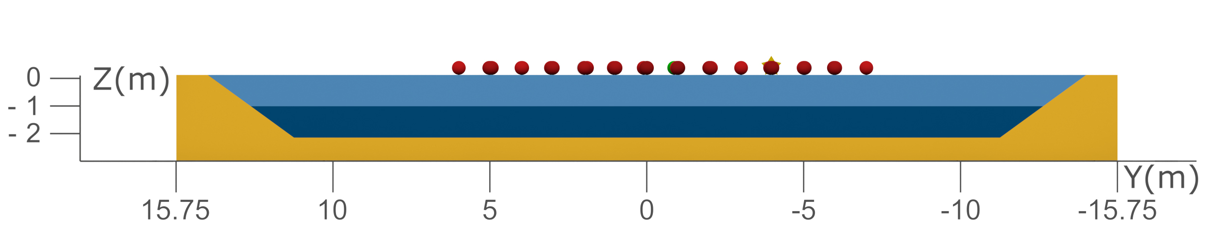
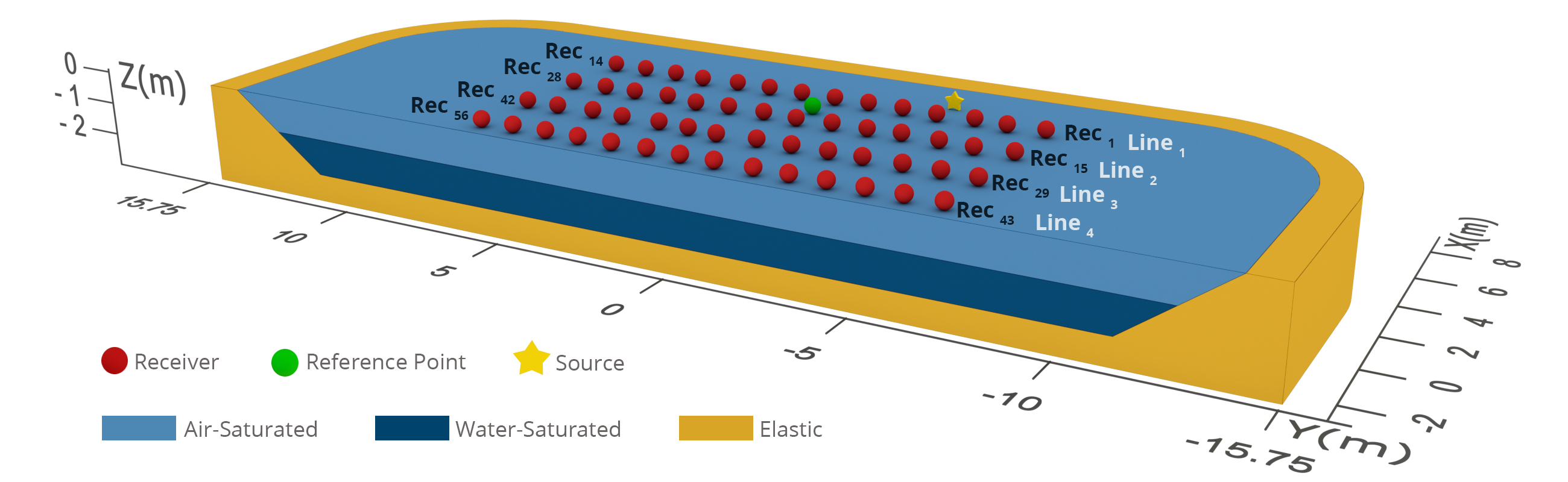
Figure 2: A schematic of the problem geometry with the top showing cross-section and the bottom an oblique angle 3D view. Light-blue color refers to air-saturated and dark-blue to water-saturated zone. Light-brown color denotes the surrounding elastic material. The setup contains a total of 57 receivers, marked with red dots and one green dot, all of which are located on the ground surface. The green dot serves as the reference receiver and is located between seventh receiver on lines 1 and 2. The source location is marked with a yellow star and placed close to the fourth receiver on line 1.

We assume a free boundary condition on the top surface while other boundaries are modeled as absorbing boundaries. In addition, we have a total of 57 receivers, which will capture the solid velocity components $v_{\rm s}$ and $w_{\rm s}$. Exact receiver locations were accurately surveyed using a cm accuracy commercially available differential (DGPS) system, and these locations are used in the numerical modeling. One extra receiver, illustrated by a green color, is located between lines 1 and 2 and is used as a reference point. A more detailed discussion of the reference point is given later in Section 4.1.

Although the acquisition involved 13 shot locations, the inversion is based on data from a single source location only. The location for the source was arbitrarily selected to be the closest to receiver 4 on Line 1. The seismic source is modeled as a vertical force pointing to the negative $z$-axis. Since the exact location of the source slightly varies between different measurements (distance from the closest geophone was measured with a ruler), the location was assumed to be uncertain in the numerical model when training the neural network. In practice, the source center location in the $(x,y)$-plane is randomized from $x\sim\rm{unif}(4.4890,4.5890)$ and $y\sim\rm{unif}(-5.2142,-5.1142)$ m. Receivers and the source are placed on the ground surface.

As a source function, we use a first derivative of a Gaussian

$$g=\frac{(t-t_{0})}{c}\exp\left(b\left(\left(t-t_{0}\right)^{2}-c^{2}\right)\right),$$ (1)

where $b=-(f\pi)^{2}$ and $c=\sqrt{-0.5/b}$. When creating the training data, we set frequency $f$ to 60 Hz, time delay $t_{0}$ to $1.2/f$, and modelling time to 0.35 s.

3.2 Physical parameters

The parameters defining the viscoelastic material are based on solid density $\rho_{\mathrm{e}}$, pressure wave speed $c_{P}$, shear wave speed $c_{S}$, and quality factors $Q_{P}$ and $Q_{S}$. The quality factors define the level of viscous attenuation in the medium. In the current paper, these parameters are randomized from uniform distributions, and minimum and maximum values are given in Table 1. One must note, that the attenuation is modeled with three mechanisms in both porous reservoir and the surrounding medium, see [12].

Table 1: Material parameter bounds assumed for the elastic material.

variable name	symbol (unit)	Minimum value	Maximum value
Solid density	$\rho_{\mathrm{e}}$ (kg/m3)	1400	1800
Pressure wave speed	$c_{P}$ (m/s)	1000	2000
Shear wave speed	$c_{S}$ (m/s)	400	800
Quality factor	$Q_{P}$	20	50
Quality factor	$Q_{S}$	20	50

The fluid parameters for the water-saturated subdomain are given by: the density $\rho_{\mathrm{f}}=1000$ kg/m³, the fluid bulk modulus $\kappa_{\mathrm{f}}=2.1025$ GPa, and the viscosity $\eta=1.14$e-3 Pa$\cdot$s, while in the air-saturated part, we set: $\rho_{\mathrm{f}}=1.2$ kg/m³, $\kappa_{\mathrm{f}}=1.3628$e5 Pa, and $\eta=1.8$e-5 Pa$\cdot$s. The quality factor $Q_{\kappa_{\mathrm{f}}}$ is set to $\infty$. All other material parameters of the water storage reservoir are assumed to be random. These parameters are randomized from uniform distributions. Minimum and maximum values are given in Table 2.

Permeability $k$ is calculated from the Darcy law

$$\frac{k}{\eta}=\frac{K}{\rho_{f}g},$$ (2)

where $g=9.81$ m/s². In this work, the hydraulic conductivity $K$ is approximated from [4]

$$K\,(\mbox{m/s})=a\left(I_{0}+0.025\left(d_{50}-d_{10}\right)\right)^{2},$$ (3)

where $a=1300/(24\cdot 60^{2})$ and $I_{0}$ is the intercept of the line formed by grain-size values with the grain-size axis. Minimum and maximum values for the grain-size parameters $d_{10}$ and $d_{50}$ are given in Table 2. We compute the permeability value for each material sample using the viscosity and density values for water.

Table 2: Material parameter bounds assumed for the water reservoir.

variable name	symbol (unit)	Minimum value	Maximum value
Mass density of sand grains	$\rho_{\mathrm{s}}$ (kg/m3)	2400	2800
Solid bulk modulus	$\kappa_{\mathrm{s}}$ (GPa)	45	55
Frame bulk modulus	$\kappa_{\mathrm{fr}}$ (GPa)	0.008	0.05
Frame shear modulus	$\mu_{\mathrm{fr}}$ (GPa)	0.002	0.04
Tortuosity	$\tau$	1.1	1.8
Porosity	$\phi$ ($\%$)	30	40
Quality factor	$Q_{\mu_{\mathrm{fr}}}$	15	50
Quality factor	$Q_{\kappa_{\mathrm{s}}}$	80	120
Quality factor	$Q_{\kappa_{\mathrm{fr}}}$	15	50
Grain-size	$d_{10}$ (mm)	0.4	0.8
Grain-size	$d_{50}$ (mm)	1.1	1.6

The volume of stored water in the reservoir can be calculated by multiplying the volume of the water-saturated domain by the porosity. In this paper, the amount of water is calculated only from the water-saturated zone that is located exactly under the array of receivers. In general, the accurate estimation of water volume is possible in water-saturated subdomain with the current problem setup, however, this cannot be principally assumed in more realistic aquifer models.

3.3 Computing of seismic data

In this research, we utilize an in-house software that is based on the discontinuous Galerkin (DG) method [10] and the third-order Adams-Bashforth time-stepping [8] techniques to generate synthetic seismograms. Our software employs tetrahedral elements to discretize the geometry of the problem. In addition to the element size, the accuracy can be controlled by selecting the order of the polynomial basis functions. For an in-depth discussion of the applied software and the associated methodology, we refer to [12] and references therein.

4 Neural network-based characterization of water storage

4.1 Noise model and source function normalization

Following [12] and denoting the measurement data vector and forward model as $\Upsilon=[v_{\rm s},w_{\rm s}]^{\top}$ and $\mathcal{A}$ respectively, the observation model is given by

$$\Upsilon=\mathcal{A}(\bm{m})+e=X+e,$$ (4)

where $\bm{m}$ contains all the physical and geometrical parameters of the model and $e$ accommodates additive noise components. The forward operator $\mathcal{A}$ is used to map the model parameters $\bm{m}$ to the seismic data vector, simulated using the coupled viscoelastic-poroviscoelastic material model by the DG method in three dimensions [7, 12].

To approximate the measurement noise in the field measurements, we apply the following noise model

$$X_{\ell}^{\textrm{noised}}=X_{\ell}+A|X_{\ell}|_{\max}\epsilon^{A}+B|X_{\ell}|\epsilon^{B},$$ (5)

where $\epsilon^{A}$ and $\epsilon^{B}$ represent independent zero-mean Gaussian random variables. $|X_{\ell}|_{\max}$ is the maximum absolute value of the $\ell$’th sample. The two noise components correspond to additive white noise and amplitude-related noise, respectively, contributing to a diverse range of noise levels. By adjusting $A$ and $B$ within the intervals $[0.05,2]\%$ and $[0,2]\%$ consecutively, wide noise variations are introduced.

As discussed in Section 2.2, the field data was measured for 3 seconds. We estimated the standard deviation of the Gaussian white noise component by analyzing the measured data within a time window spanning from 1 second to 2 seconds. Subsequently, we compared this estimated value to the maximum amplitudes observed in the traces. This gave an approximation of the noise level in the real data ($A_{\rm{meas}}\approx 0.4\%$) and the applied noise levels in model (5) covers such value. The selection for parameter $B$ interval is arbitrary.

In order to obtain a source-independent inversion, we use a deconvolution operation to remove the effect of the seismic source time function. We transform the transient signals to the frequency domain and use data from a reference point, which is an additional receiver (see Fig. 2), as the system response function. This allows us to change the original observation model (Eq. (4)) with a new formulation

$$\frac{F(\Upsilon)}{F(\Upsilon_{\rm ref})}=\frac{F(X)}{F(X_{{\rm ref}})}+\hat{e},$$ (6)

where $F$ represents the Fourier transform in time, and the subscript ”ref” denotes the data from the reference point. The quantity $\hat{e}$ represents the noise in the frequency domain formulation after normalization. However, (6) can become ill-conditioned when the denominator approaches zero. To address this issue, we adopt the Wiener filtering approach for regularization, as proposed in [18].

4.2 Examples of real and synthetic seismic data

Figure 3 presents a sample shot gathered from the real dataset, displaying the $v_{\rm s}$ and $w_{\rm s}$ velocity components along with the reference records as an example in the top right corner. The bottom row shows the real and imaginary parts of the Fourier transformed and source function normalized records, which serve as inputs to the neural network. For the shown data, water table level was at $-88.7$ cm.

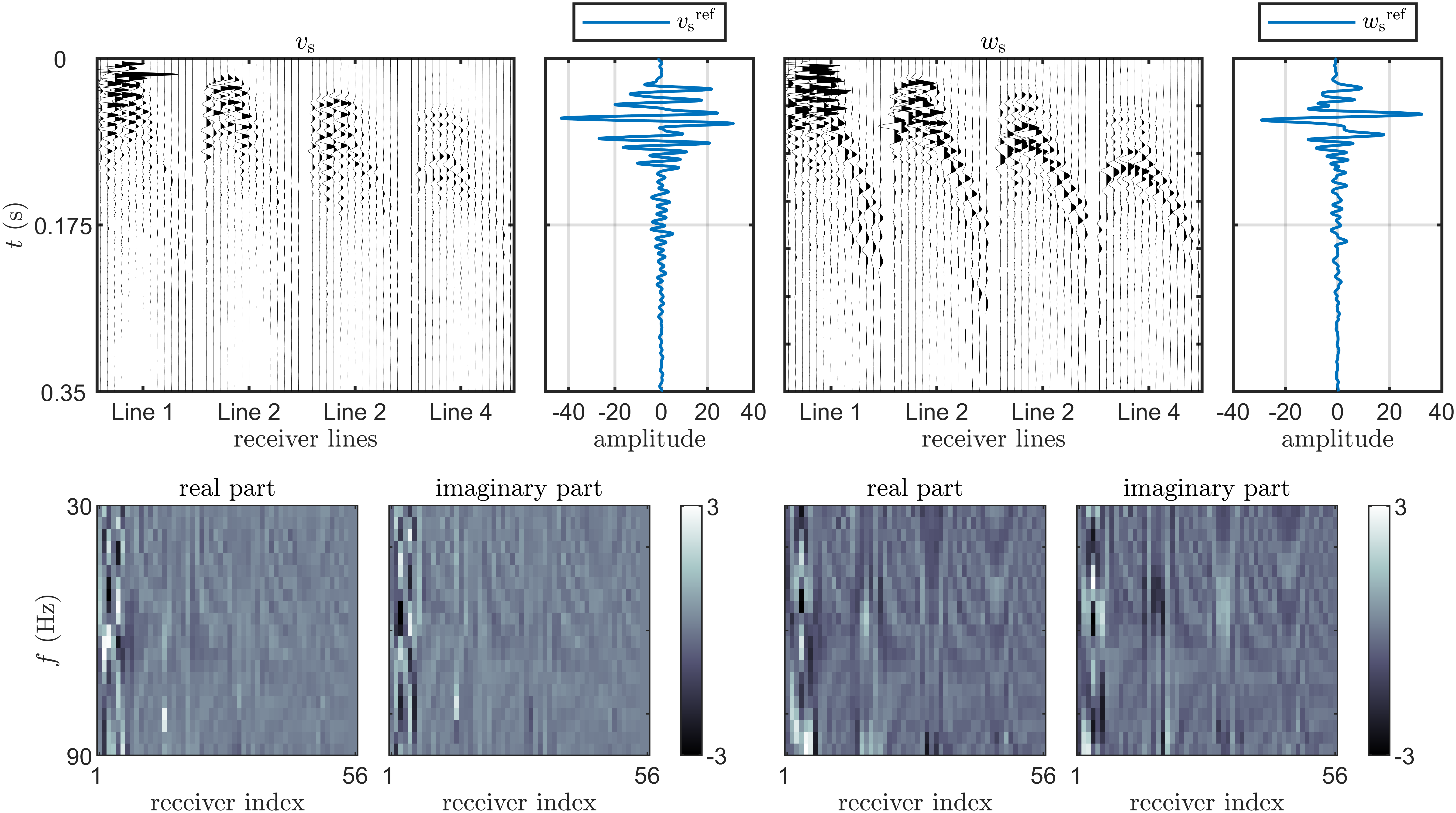
Figure 3: An example of the measured data. The figures on the left show the $v_{\rm s}$ component, and the figures on the right the $w_{\rm s}$ component. The velocity components on the reference point are shown to illustrate the data behaviour.

Figure 4 shows an example of the simulated data. Here the water table level was at $-72.10$ cm and the noise level parameters were set to $A=1\%$ and $B=1\%$. The discrepancy between measured and synthetic seismograms in these figures is due to the random selection of material parameters employed in generating the synthetic data.

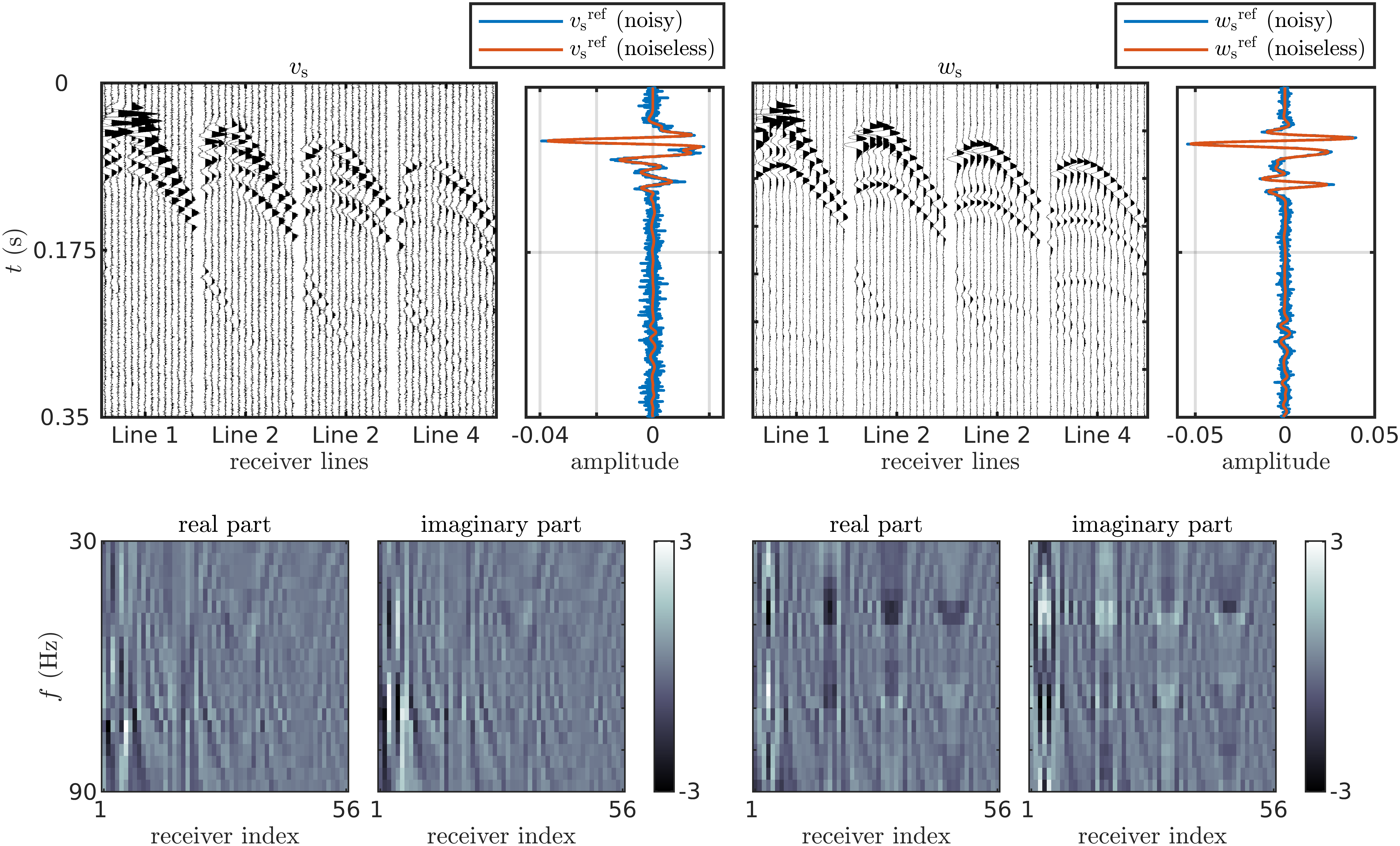
Figure 4: An example of the synthetic data. The pictures on the left show the $v_{\rm s}$ component, and the figures on the right the $w_{\rm s}$ component. The reference data traces on the top panel are shown for the noisy and noiseless data for both velocity components.

4.3 Neural networks

We generated 15,000 training and 3,000 validation samples using fifth-order polynomials and the source wavelet (1) with the DG solver. The inviscid material model-based element size criterion is approximately 1.9 elements per shortest wavelength for the samples in the validation dataset and 2.0 for training dataset samples.

A fully connected neural network was employed in this study to determine the water volume using seismic data. We down-sample the synthetic data to the sampling frequency of 4 kHz, then five copies of clean training and validation databases are corrupted with Gaussian noise according to the noise model in (5). The time domain data are transformed to the frequency domain and the corresponding real and imaginary components are used as inputs to the network. We select 21 frequencies between 30 to 90 Hz, see Figs. 3 and 4 as examples.

The training uses the TensorFlow [3] and Keras [6] libraries. We use the Adam optimizer [13] and the RandomSearch algorithm of the Keras Tuner library [16] which maximizes the model’s behavior given the training and validation datasets by testing different hyperparameters in different random combinations. We allow Keras Tuner to randomize the activation function, learning rate, number of hidden layers, number of neurons per hidden layer, and L2 regularization penalty factor. Our choices for activation function, are “relu”, “sigmoid”, “tanh”, “selu”, “swish”, or “LeakyReLU” and number of hidden layers from one to six. The number of neurons varies from 100 to 5,000, and for the learning rate, we allow Keras Tuner to choose from [1e-3, 1e-4, 1e-5], and L2 regularization penalty from [1e-5, 1e-6, 1e-7, 1e-8]. For all networks studied in this work, the batch size is set to 256.

In this study, the best-performing network is selected according to mean absolute error (MAE) with validation. After testing the different hyperparameter combinations explained above, the network is made up of five hidden layers with 2,570 (layer 1), 3,920 (layer 2), 3,360 (layer 3), 2,730 (layer 4), and 3,400 (layer 5) neurons, a LeakyRelu activation function, a learning rate of 1e-5, and L2 regularization penalty factor of 1e-5. Linear activation is used for the output layer, and early stopping is also activated both in the hyperparameter tuning and actual training phases.

5 Results

All results, i.e. the simulation of wave fields and estimation of water volumes via neural networks, were computed using the computer cluster Puhti at the CSC – IT Center for Science Ltd, Finland. A detailed description of the supercomputer Puhti can be found from the CSC’s website [1]. Computational grids used in this work were build using COMSOL Multiphysics.

The results are promising in terms of estimation accuracy. Notably, the estimation accuracy for the full receiver setup aligns closely with the true values and that of the sup- plementary synthetic database. However, it’s worth mentioning that one of the field data samples produced a significantly biased estimate when compared to the true value. Closer analysis of the data traces showed that the biased sample exhibited distinct differences, particularly in terms of the RMSE.

5.1 Predictions of water volume

We test the applicability of the trained neural network model via two different test dataset. These datasets are defined as

• Field Measurements: Field data have been assessed at seven distinct water table levels, ranging from a depth of -31.3 cm to -88.7 cm. For each water level, we collected three repeated measurements from three different drop heights. These lead to a dataset consisting of a total of $3\times 3\times 7=63$ samples. Using our knowledge of the actual water table level and the geometry of the sand pool, we can calculate the volume of the water-saturated zone. Additionally, based on a previous study [17], we assume the nominal porosity of the material to be 35%.

• Synthetic Dataset: This database contains a total of 3,000 samples. We used the same prior to randomize material parameters as in the training and validation databases. Instead of randomizing the noise parameters $A$ and $B$ in (5), we set them to $1\%$ each, representing moderate noise levels. To introduce varying numerical noise in the data compared to the training and validation databases, we used a mesh density criteria of 2.5 elements per wavelength, fourth-order basis functions, and a Ricker wavelet as the source function, defined as

  $$g=(1+2b(t-t_{0})^{2})\exp\left(b\left(t-t_{0}\right)^{2}\right).$$ (7)

  The parameter $b$ and time delay $t_{0}$ are defined as for wavelet (1).

The Keras Tuner-optimized network architecture undergoes ten training runs, and the final water volume per sample result is determined as the average of these ten estimates. Figure 5 presents a comparison between the estimated (average) water volumes and their corresponding true values. The results for all drop heights are shown with different colors, red color denotes the repeated measurements from drop height 5 cm ($\rm{dh}_{5}^{1,2,3}$), green drop height 10 cm ($\rm{dh}_{10}^{1,2,3}$), and blue drop height 15 cm ($\rm{dh}_{15}^{1,2,3}$). To get a crude approximation for the uncertainty, we assumed that the porosity value in the field measurements database is uncertain in a sense that we assumed $\phi_{\rm{true}}\in[0.95,1.05]\cdot 35\%$, that can be used to compute the error bars shown for each estimate with real data. Figure shows also the estimates for the synthetic dataset. These results demonstrate the potential of using proposed neural network based approach to recover the water volume.

Figure 5: Left: Estimated volumes of water as a function of true value. Right: Histogram of relative prediction errors.

The results at water table level -36.2 cm reveal a clear outlier in Fig. 5. To analyze the differences between repeated measurements, we utilize the root mean square error (RMSE). Let $d_{i}^{k}$ represent the normalized seismic data (see model (6)) for the $k$’th repeated measurement at drop heights $i\in\{5,10,15\}$ in the frequency domain, with the real and imaginary components stacked. The RMSE error can now be expressed as follows:

$${\rm RMSE}^{\ell-j}_{i}=\frac{\|d^{\ell}_{i}-d^{j}_{i}\|_{2}}{\sqrt{N}},$$ (8)

where $\ell$ and $j$ are the indices for repeated measurements, and $N$ is the total number of values in the data vector. Table 3 lists the RMSE values between all possible combinations of input data. Specifically, the first drop height ($i=5$) exhibits significantly larger variations compared to the other two measurements. Additionally, the combination of drop iterations $\ell=2$ and $j=3$ yields comparable RMSE values for the measurements at $i=10$ and $i=15$.

Table 3: Root mean square errors (8) for different data combinations for measurements taken at a water table level of -36.2 cm.

$i$	$\ell=1,j=2$	$\ell=1,j=3$	$\ell=2,j=3$
5	15.3900	15.4115	6.2091
10	6.3498	8.5541	4.8954
15	5.8354	6.5009	4.7365

5.2 SHAP analysis

We applied Shapley Additive Explanations (SHAP) analysis to the full receiver array neural network model to determine the significance of each receiver in estimating water volume. Determining Shapley values is an attribution problem, which means it involves determining the contribution of the prediction scores of a model for a specific sample input to its base features—in our case, the receivers. In simple terms, attribution to a base feature represents the importance of that feature to the prediction. For example, when attribution is applied to a model that estimates water volume, it helps us understand how influential each receiver is in determining the water volume.

10,000 randomly selected samples from the training dataset are used to train the deep explainer model for the SHAP software [15]. The explainer model is then applied to all samples in the field measurements database. After calculating the Shapley values, we compute the normalized mean absolute values for each receiver (see top panel of Fig. 6). The results for water volume indicate that the most contributing receivers are those closest to the seismic source. For comparison, we also applied the explainer model to 1,000 randomly selected samples from the synthetic database, revealing a similar distribution of the most contributing receivers.

Next, we constructed two new receiver configurations and trained the neural network model for the field measurements based on SHAP values. For the first configuration, we selected ten receivers having the largest SHAP values, and for the second configuration, we randomly selected ten receivers from the full sensor array (see bottom panel of Fig. 6). The KerasTuner optimized network with SHAP analysis-based receiver selection consists three hidden layers with 3,490 (layer 1), 3,780 (layer 2), and 2,580 (layer 3) neurons, a LeakyRelu activation function, a learning rate of 1e-4, and L2 regularization penalty factor of 1e-6. Similarly for the randomly selected receiver selection lead to optimized network with two hidden layers with 3,490 (layer 1) and 2,580 (layer 2) neurons, a LeakyRelu activation function, a learning rate of 1e-4, and L2 regularization penalty factor of 1e-6.

Figure 7 displays the estimated water volume as a function of the true water volume for both receiver configurations. The field measurement results reveal a significant impact on estimation accuracy when employing SHAP analysis-based receiver selection compared to random selection. However, with a synthetic database, this effect is not that significant.

Figure 6: Normalized average absolute Shapley values for predicting water volume from seismic data. The results for the test and real datasets are displayed. Higher Shapley values are correlated with receivers that are closer to the seismic source.

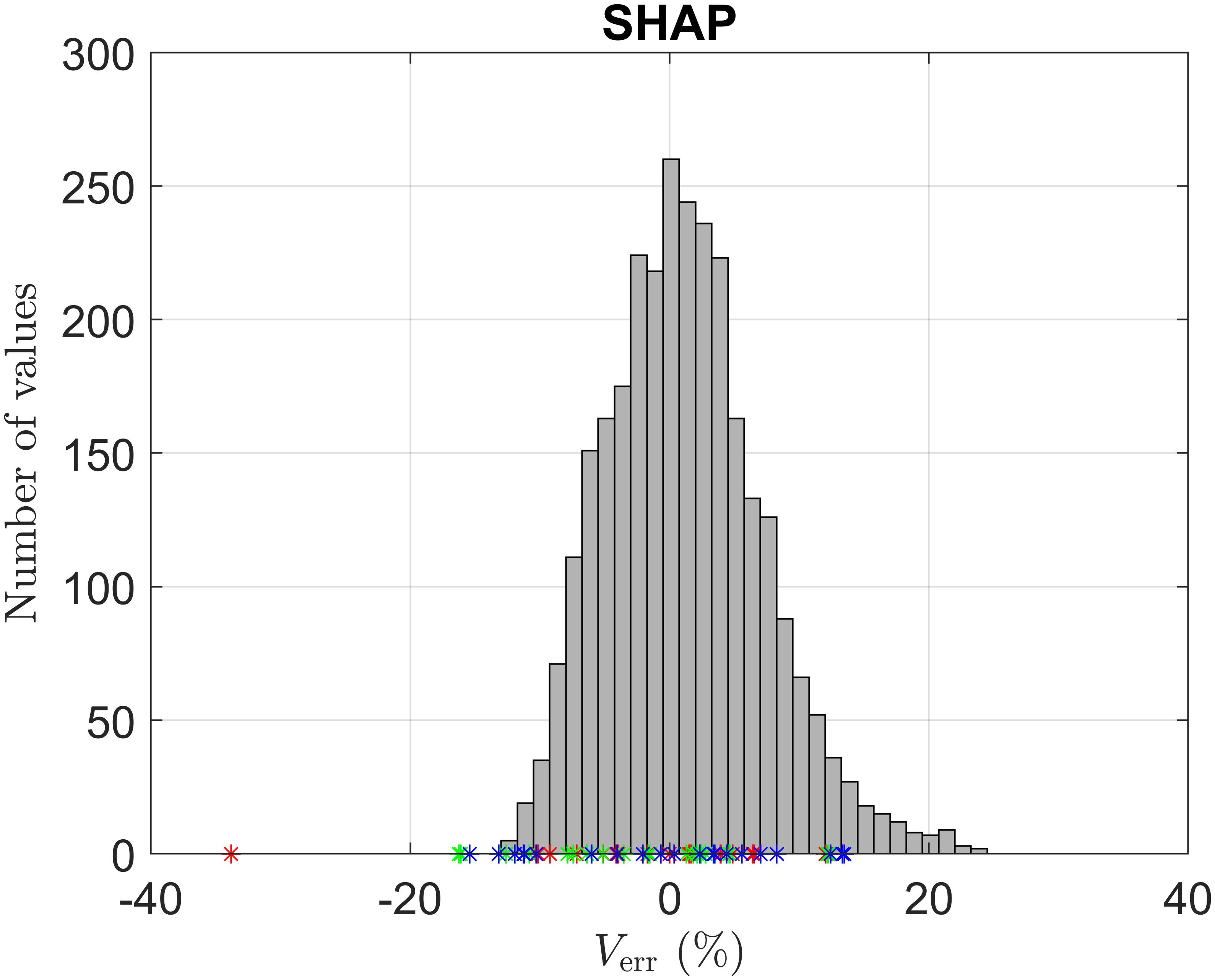
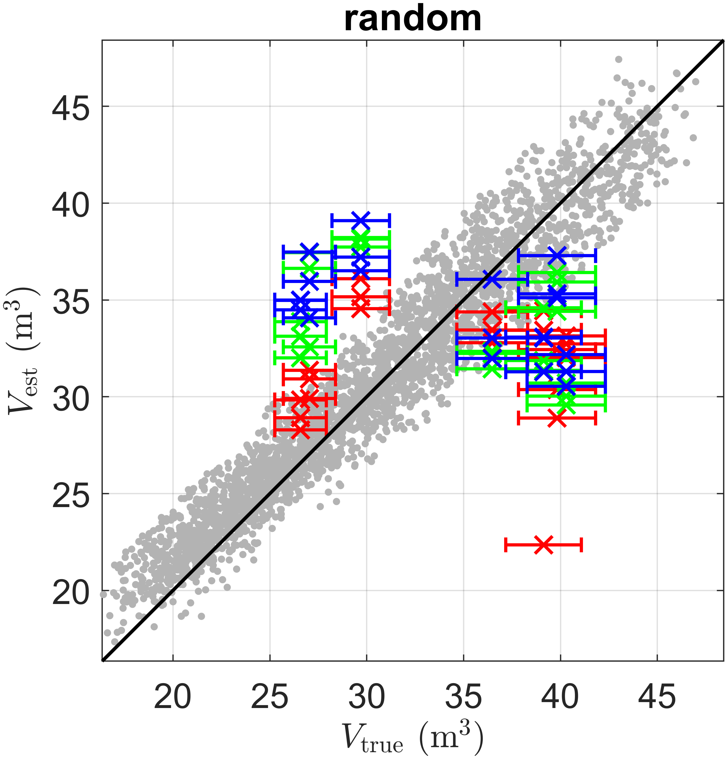
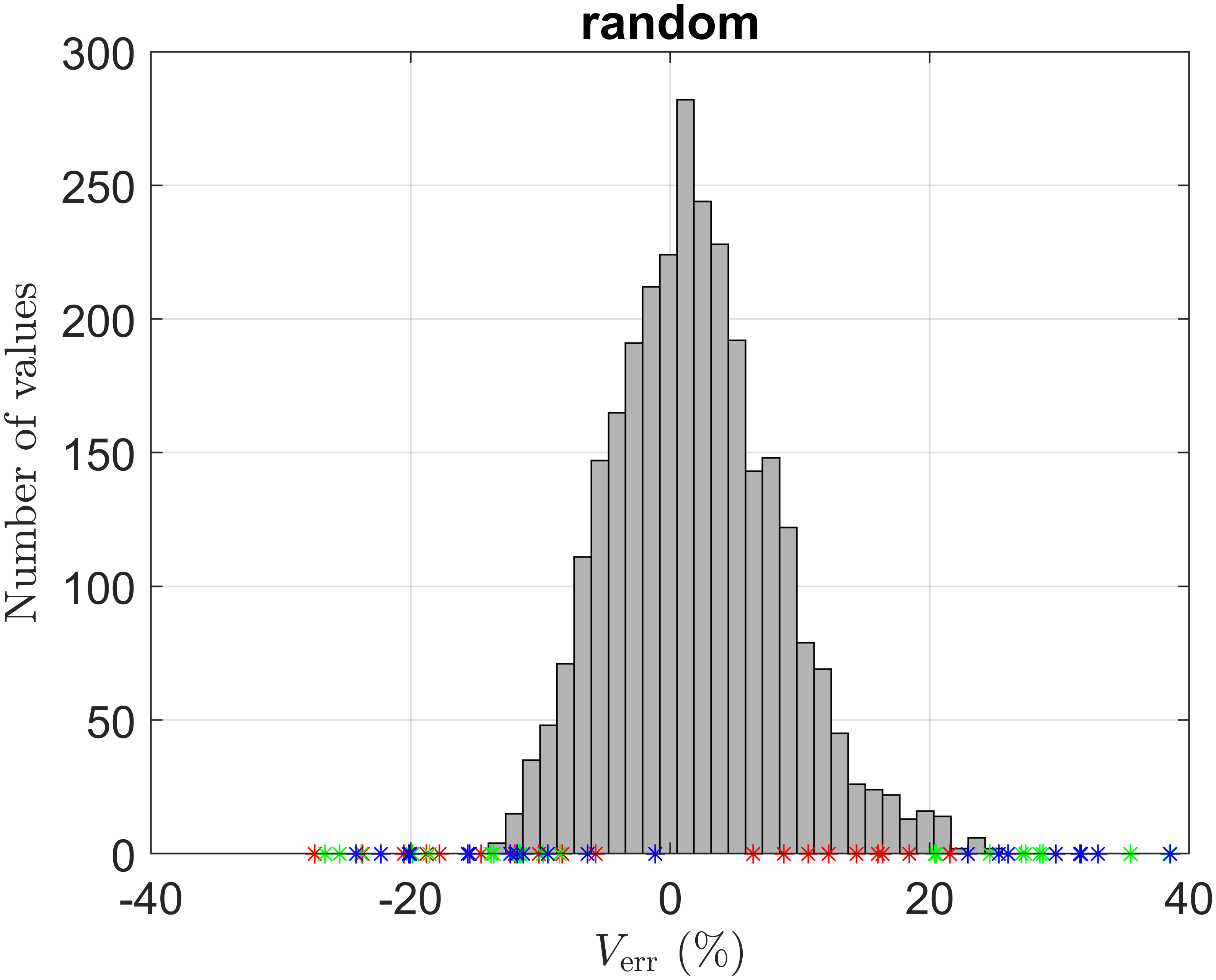
Figure 7: Left: Estimated volumes of water as a function of true value. Right: Histogram of relative prediction errors. Top panel shows the results for receiver configuration based on SHAP analysis and bottom panel for the randomly chosen receivers.

The NMB, MAE and RMSE are used as evaluation metrics to quantitatively analyze the estimation results for all three receiver configurations, see Table 4. The table shows that the full receiver array results in the most accurate measures.

Table 4: The normalized mean biases (NMB), mean absolute errors (MAE), and root mean square errors (RMSE) were computed for both field measurement and synthetic test databases. It is important to note that, instead of averaging estimates from ten randomly initialized network trainings, they were treated as individual samples in this table. The first two rows show the results for the full receiver array, the following two lines for the ten receivers found most contributing according to SHAP analysis, and the last two rows the results for ten receivers selected randomly.

Receiver array setup	Database	NMB (%)	MAE (m3)	RMSE
full	field meas.	1.2604	2.3259	2.9787
	synthetic	1.5976	1.3801	1.7174
SHAP	field meas.	-1.3241	3.2449	4.1318
	synthetic	0.5348	1.5146	1.8950
random	field meas.	-2.3320	6.5112	7.2178
	synthetic	1.2344	1.5768	1.9630

6 Discussion and Conclusions

In this study, we investigated the water volume estimation from seismic data. The field measurements were done for a reservoir for which the water table level is controllable and known. Furthermore, we possessed accurate knowledge of the reservoir’s geometry and physical characteristics. Our approach involved testing the field data against a proposed neural network model, developed through a training phase utilizing synthetic data.

The physical model for synthetic wave propagation computations was a coupled poroviscoelastic–viscoelastic system. The wave propagation problem was solved on a GPU cluster using the nodal DG method coupled with the Adams-Bashforth time-stepping scheme to generate synthetic seismograms. In the synthetic model, the material was assumed to be homogeneous, and the water table level was allowed to move freely within the geometry.

For the inverse problem, we employed a fully connected neural network to estimate water volume from seismic data. The databases used during the training phase were synthetically generated using a wave propagation solver. The training data were corrupted with noise at levels similar to those found in real data. In our proposed approach, the source wavelet is unknown, and we employ a deconvolution-based method to normalize the source function. The input data for the neural network consisted of seismic data in the frequency domain.

A crucial element of our research was the examination of how closely the estimations from seismic data matched with the actual water volumes and water table levels in the controlled reservoir environment. These correlations are key to verifying the accuracy of our neural network model. Quantitative comparison between the seismic data-derived estimates with the ground truth of the reservoir’s water levels and volumes is fundamental to demonstrating the reliability of our approach. It is especially pertinent when considering the potential application of our methods in varied and uncontrolled real-world scenarios.

In this study, we computed the average absolute SHAP values at the receiver level for the field data. Since SHAP values provide insight into which of the receivers contributes the most to the estimates, we tested the estimation accuracy by selecting the ten most contributing receivers and repeating the estimation procedure. In this case, the network was re-optimized using Keras Tuner tools. Additionally, we tested the estimation accuracy by selecting receivers randomly. For the randomly selected receivers, we used the same network as was used for SHAP value-based selection. It was observed that the estimation accuracy was significantly affected when randomly selected receivers were used. On the other hand, the accuracy between the full array and SHAP value-based selection methods was similar. For synthetic data, the effect on estimation accuracy was not as dramatic when randomly selected receivers were used.

Future research should encompass larger test sites with heterogeneous materials. From a methodological perspective, approaches to provide insights into the estimation uncertainty, as well as methods to normalize the source wavelet in time, could be potential research directions. Furthermore, depending on the characteristics of the site under investigation, it may be necessary to extend the current physical models. These extensions could involve accommodating anisotropic materials, addressing issues related to partial saturation, and incorporating more complex noise models.

In this study, synthetic databases were constructed using a single arbitrarily selected source location from field measurements. Future research could explore the inclusion of multiple sources, particularly beneficial for addressing challenges associated with complex geometries and material inhomogeneities.

Appendix A Measured data, water table level -36.2 cm

In this section, the data is shown for all measurements from drop height 5 cm at the water table level -36.2 cm. Notably, the first measurement within this series led to biased water volume estimate, as elaborated in Section 5.1.

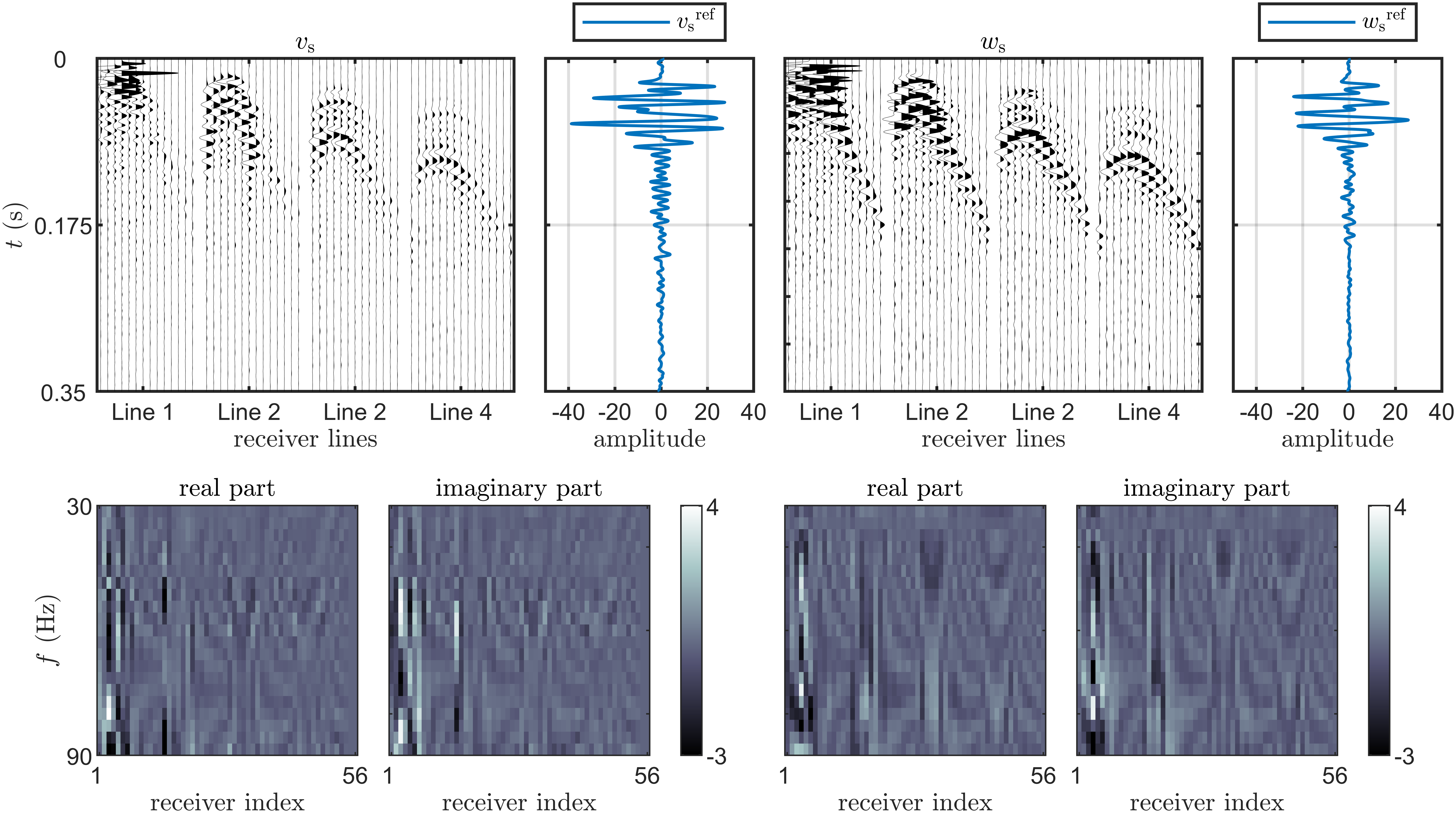
Figure 8: The figure depicts measured data traces, with the top panels displaying results in the time domain and the bottom panels showing the corresponding data converted into the frequency domain. These measurements were taken at a water table level of -36.2 cm. Specifically, the figure presents the initial measurement out of a series of three, all conducted from a drop height of 5 cm.

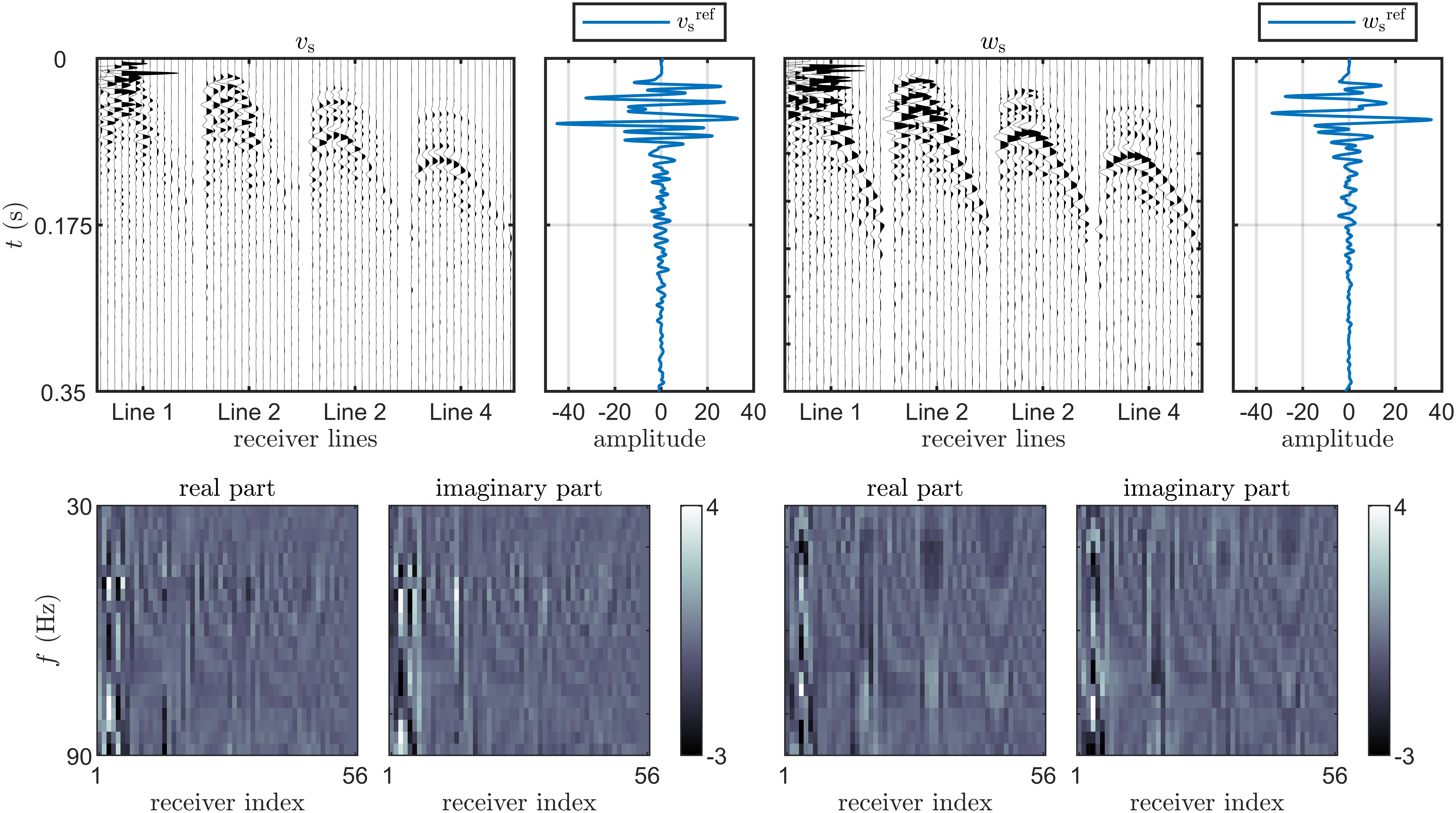
Figure 9: Otherwise the same caption as in Fig. 8, but the data is for the second iteration of measurements.

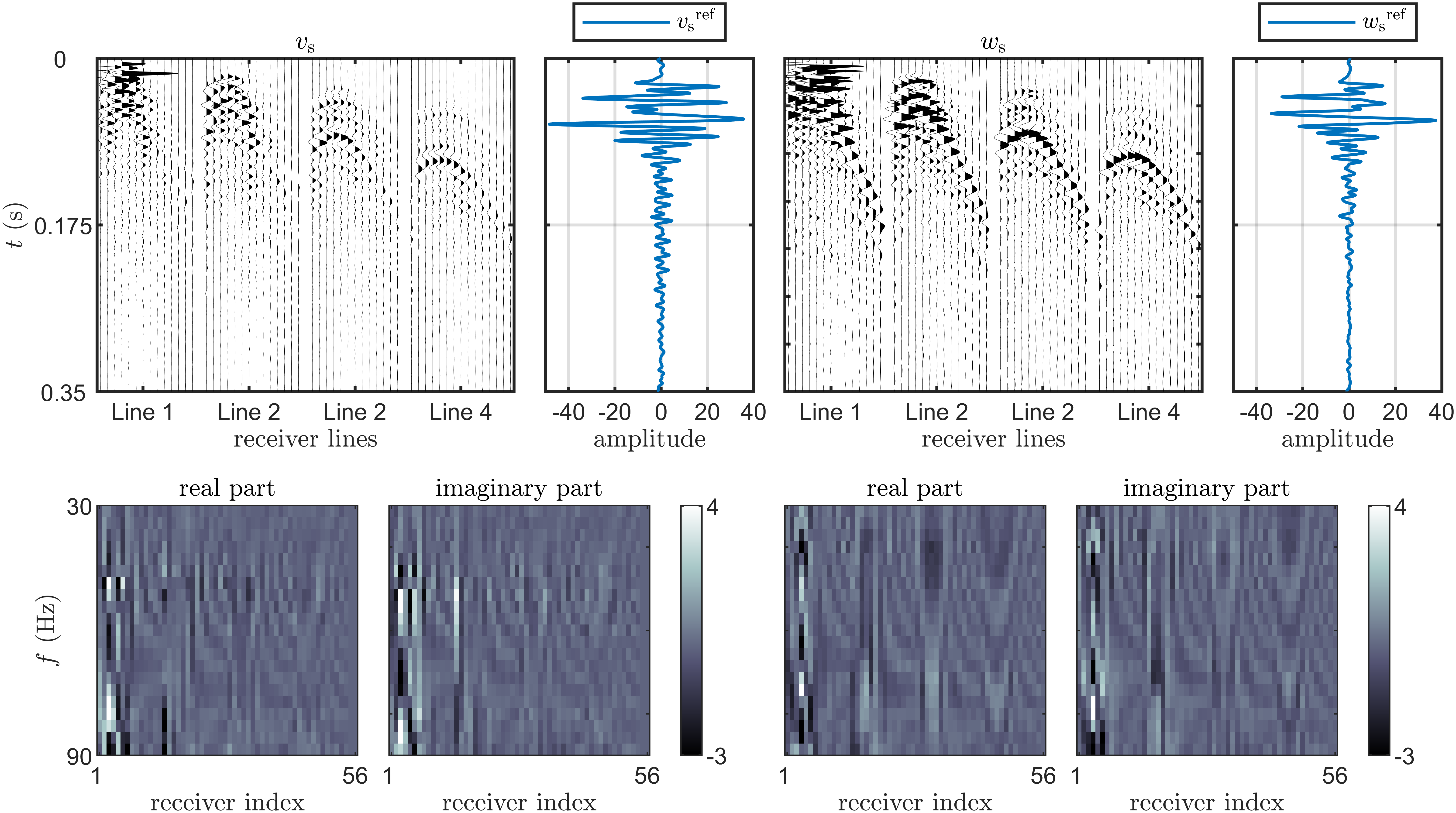
Figure 10: Otherwise the same caption as in Fig. 8, but the data is for the third iteration of measurements.

References

- [1] CSC – IT Center for Science Ltd, Computing environment Puhti. https://docs.csc.fi/computing/systems-puhti/. Accessed: Oct. 7, 2023.
- [2] FLEX EPOS. https://wiki-emerita.it.helsinki.fi/display/FLEX/Large-N+Devices. Accessed: Dec. 21, 2023.
- [3] M. Abadi, A. Agarwal, P. Barham, E. Brevdo, Z. Chen, C. Citro, G. S. Corrado, A. Davis, J. Dean, M. Devin, S. Ghemawat, I. Goodfellow, A. Harp, G. Irving, M. Isard, Y. Jia, R. Jozefowicz, L. Kaiser, M. Kudlur, J. Levenberg, D. Mané, R. Monga, S. Moore, D. Murray, C. Olah, M. Schuster, J. Shlens, B. Steiner, I. Sutskever, K. Talwar, P. Tucker, V. Vanhoucke, V. Vasudevan, F. Viégas, O. Vinyals, P. Warden, M. Wattenberg, M. Wicke, Y. Yu, and X. Zheng. TensorFlow: Large-scale machine learning on heterogeneous systems, 2015. Software available from tensorflow.org.
- [4] M. S. Alyamani and Z. Sen. Determination of hydraulic conductivity from complete grain-size distribution curves. Groundwater, 31(4):551–555, 1993.
- [5] J. Carcione. Wave Fields in Real Media: Wave propagation in anisotropic, anelastic and porous media. Elsevier, 2015.
- [6] F. Chollet et al. Keras. https://keras.io, 2015.
- [7] N. F. Dudley Ward, S. Eveson, and T. Lähivaara. A discontinuous Galerkin method for three-dimensional poroelastic wave propagation: Forward and adjoint problems. Computational Methods and Function Theory, 21:737–777, 2021.
- [8] D. R. Durran. The third-order Adams-Bashforth method: An attractive alternative to leapfrog time differencing. Monthly Weather Review, 119:702–720, 1991.
- [9] M. Giordano. Global groundwater? issues and solutions. Annual review of Environment and Resources, 34:153–178, 2009.
- [10] J. S. Hesthaven and T. Warburton. Nodal Discontinuous Galerkin Methods: Algorithms, Analysis, and Applications. Springer, 2007.
- [11] P. Kearey, M. Brooks, and I. Hill. An Introduction to Geophysical Exploration, volume 4. John Wiley & Sons, 2002.
- [12] M. Khalili, P. Göransson, J. S. Hesthaven, A. Pasanen, M. Vauhkonen, and T. Lähivaara. Monitoring of water volume in a porous reservoir by seismic data: A 3D simulation study. arXiv preprint arXiv:2211.14276, 2022.
- [13] D. P. Kingma and J. Ba. Adam: A method for stochastic optimization. arXiv.org perpetual, non-exclusive license, 2014.
- [14] T. Lähivaara, A. Malehmir, A. Pasanen, L. Kärkkäinen, J. M. Huttunen, and J. S. Hesthaven. Estimation of groundwater storage from seismic data using deep learning. Geophysical Prospecting, 67(8):2115–2126, 2019.
- [15] S. M. Lundberg and S.-I. Lee. A unified approach to interpreting model predictions. Advances in neural information processing systems, 30, 2017.
- [16] T. O’Malley, E. Bursztein, J. Long, F. Chollet, H. Jin, L. Invernizzi, et al. Kerastuner. https://github.com/keras-team/keras-tuner, 2019.
- [17] J. T. Pulkkinen, A.-K. Ronkanen, A. Pasanen, S. Kiani, T. Kiuru, J. Koskela, P. Lindholm-Lehto, A.-J. Lindroos, M. Muniruzzaman, L. Solismaa, et al. Start-up of a “zero-discharge” recirculating aquaculture system using woodchip denitrification, constructed wetland, and sand infiltration. Aquacultural Engineering, 93:102161, 2021.
- [18] W. Wen and E. Kalkan. System identification based on deconvolution and cross correlation: An application to a 20-story instrumented building in Anchorage, Alaska. Bulletin of the Seismological Society of America, 107(2):718–740, 2017.