Non-Denoising Forward-Time Diffusions
Abstract
The scope of this paper is generative modeling through diffusion processes. An approach falling within this paradigm is the work of Song et al. (2021), which relies on a time-reversal argument to construct a diffusion process targeting the desired data distribution. We show that the time-reversal argument, common to all denoising diffusion probabilistic modeling proposals, is not necessary. We obtain diffusion processes targeting the desired data distribution by taking appropriate mixtures of diffusion bridges. The resulting transport is exact by construction, allows for greater flexibility in choosing the dynamics of the underlying diffusion, and can be approximated by means of a neural network via novel training objectives. We develop a unifying view of the drift adjustments corresponding to our and to time-reversal approaches and make use of this representation to inspect the inner workings of diffusion-based generative models. Finally, we leverage on scalable simulation and inference techniques common in spatial statistics to move beyond fully factorial distributions in the underlying diffusion dynamics. The methodological advances contained in this work contribute toward establishing a general framework for generative modeling based on diffusion processes.
1 Introduction
Denoising diffusion probabilistic modeling (DDPM) (Sohl-Dickstein et al., 2015; Ho et al., 2020; Song et al., 2021) is a recent generative modeling paradigm exhibiting strong empirical performance. Consider a dataset of samples with empirical distribution . The unifying key steps underlying DDPM approaches are: (i) the definition of a stochastic process with initial distribution , whose forward-time (noising) dynamics progressively transform toward a simple data-independent distribution ; (ii) the derivation of the backward-time (denoising / sampling) dynamics transforming toward ; (iii) the approximation of the backward-time transitions by means of a neural network. Following the training step (iii), a sample whose distribution approximates is drawn by (iv) simulating from the approximated backward-time transitions starting with a sample from . Both discrete-time (Ho et al., 2020) and continuous-time (Song et al., 2021) formulations of DDPM have been pursued. This work focuses on the latter case, to which we refer as diffusion time-reversal transport (DTRT). As in DTRT, dynamics are specified through diffusion processes, i.e. solutions to stochastic differential equations (SDE) with associated drift and diffusion coefficients. A number of approximations are involved in the aforementioned steps. Firstly, as the dynamics are defined on a finite time interval, a dependency from is retained through the noising process. Hence, starting with a sample from the data-independent distribution in (iv) introduces an approximation. Secondly, while the backward-time dynamics of (ii) are directly available for diffusions, they are approximated by means of a neural network in (iii). Thirdly, sampling in (iv) is achieved through a discretization on a time-grid, which introduces a discretization error. De Bortoli et al. (2021, Theorem 1) links these approximations to the total variation distance between the distribution of the generated samples from (iv) and .
In our first methodological contribution we develop a procedure for constructing diffusion processes targeting without relying on time-reversal arguments. The proposed transport (coupling) between and is achieved by: (1) specifying a diffusion process on starting from a generic ; (2) conditioning on hitting a generic at time , thus obtaining a diffusion bridge; (3) taking a bivariate mixture of diffusion bridges over with marginals and , obtaining a mixture process ; (4) matching the marginal distribution of over with a diffusion process, resulting in a diffusion with initial distribution and terminal distribution . The realized diffusion bridge mixture transport (DBMT) between and is exact by construction. We thus sidestep the approximation common to all DDPM approaches due to the dependency from retained through the noising process. Moreover, the DBMT can be realized for almost arbitrary , and . This increased flexibility is a departure from the DTRT where and need to be chosen to obtain convergence toward a simple distribution .
Similarly to the DTRT, achieving the DBMT requires the computation of a drift adjustment term which depends on . For a SDE class of interest, we develop a unified and interpretable representation of DTRT and DBMT drift adjustments as simple transformations of conditional expectations over . This novel result provides insights on the target mapping that we aim to approximate and on the quality of approximation achieved by the trained score models of Song et al. (2021). Having defined for the DBMT a Fisher divergence objective similarly to Song et al. (2021), we leverage on this unified representation to define two additional training objectives featuring appealing properties.
In our last methodological contribution we extend the class of SDEs that can be realistically employed in computer vision applications. Specifically, computational considerations have so far restricted the transitions of the stochastic processes employed in DDPM to be fully factorials. We view images at a given resolution as taking values over a 2D lattice which discretizes the continuous coordinate system representing heights and widths. Diffusion processes are viewed as spatio-temporal processes with spatial support . Doing so, it is possible to leverage on scalable simulation and inference techniques from spatial statistics and consider more realistic diffusion transitions.
This paper is structured as follows. In Section 2 we review the DTRT of Song et al. (2021) and in Section 3 we introduce the DBMT. In order to implement the DTRT and the DBMT it is necessary to specify the underlying SDE, i.e. the coefficients and . We study a class of interest in Section 4. The unified view of drift adjustments is introduced in Section 5. Section 6 develops the training objectives and Section 7 reviews the obtained results and finalizes the DBMT construction. In Section 8 we establish the connection with spatio-temporal processes. We conclude in Section 9. Appendices A, B, C and D contain the theoretical framework, assumptions, proofs, and additional material.
Notation and conventions: we use uppercase notation for probability distributions (measures, laws) and lowercase notation for densities; each probability distribution, and corresponding density, is uniquely identified by its associated letter not by its arguments (which are muted); for example is a distribution, is its corresponding density; random elements are always uppercase (an exception is made for times, always lowercase for typographical reasons); if is the distribution of a stochastic process, we use subscript notation to refer to its finite dimensional distributions (densities with ), conditional or not, for some collection of times; for example denotes a transition density, which is understood to be a function of four arguments ; is the delta distribution at and is used for product distributions; we refer directly to a given SDE instead of referring to the diffusion process satisfying such SDE when no ambiguity arises; we use and for vector and matrix indexing, for matrix transposition.
2 Diffusion Time-Reversal Transport
The starting point of Song et al. (2021) is a diffusion process satisfying a generic -dimensional time-inhomogenous SDE with initial distribution
| (1) |
over noising time . Thorough this paper we denote with the law of the diffusion solving 1 and with the corresponding densities. Thus, let , , be the transition density of 1, and let , , be the marginal density of 1. As , we have
| (2) |
The dynamics of 1 over the reversed, i.e. sampling, time , , are given by (Anderson, 1982; Haussmann & Pardoux, 1986; Millet et al., 1989)
| (3) |
where is the remaining sampling time, and the -dimensional vector is defined by . That is the processes and have the same distribution. Approximating the terminal distribution of 1, i.e. the initial distribution of 3, with , is sampled from and 3 is discretized and integrated over to produce a sample approximately distributed as .
The computation of the multiplicative drift adjustment entering 3, i.e. the score of the marginal density 2, requires in principle operations. Let be a neural network for which we would like . It remains to find a suitable training objective for which unbiased gradients with respect to can be obtained at cost with respect to the dataset size . As has a mixture representation, the identity of Vincent (2011) for Fisher divergences provides us with the desired objective for a fixed
| (4) |
The key point is that an unbiased, with respect to , mini-batch Monte Carlo (MC) estimator for the expectation 4 can be trivially obtained by sampling a batch , , and evaluating the average loss over the batch. In order to achieve a global approximation over the whole time interval , Song et al. (2021) proposes uniform sampling of time
| (5) |
where is a regularization term. A MC estimator for 5 is constructed by augmenting the MC estimator for 4 with the additional sampling step .
3 Diffusion Bridge Mixture Transport
Our starting point is a generic -dimensional time-inhomogenous SDE which, in contrast to Song et al. (2021), is directly defined on the sampling time
| (6) |
We reserve to denote the law of the diffusion solving 6 for a given starting value and to denote the corresponding densities.
3.1 Diffusion Bridges
Diffusion bridges are central to the proposed methodology, in this Section we cover their basic theory. A diffusion bridge is a diffusion process starting from a given value which is conditioned on hitting a terminal value. It is a deep result, and consequence of Doob -transforms (Särkkä & Solin (2019, Chapter 7.9), Rogers & Williams (2000, Chapter IV.6.39)), that a diffusion processes pinned down on both ends is still a diffusion process. In particular the Markov property is preserved. More precisely, 6 with initial value conditioned on hitting a terminal value at time is characterized the following SDE on with initial value (Särkkä & Solin, 2019, Theorem 7.11)
| (7) |
where . The multiplicative adjustment factor forces the process to hit at time and the diffusion process solving 7 is known as the diffusion bridge from to . As previously noted, in 7 refers to the transition density of 6.
3.2 Diffusion Mixtures
The proposed transport construction relies on a representation result for diffusion mixtures. We present here an informal version and report the precise statement, the required assumptions, and the proof in Appendix A.
Theorem 1 (Diffusion mixture representation — informal).
Let , be a collection of diffusions with associated SDEs and marginal densities . Let be a mixing distribution on , be the -mixture of . Then there exists a diffusion process with marginal . follows a SDE whose drift and diffusion coefficients are weighted averages of the corresponding coefficients in , where the weights are proportional to and to the mixing density.
Theorem 1 is first established in Brigo (2002, Corollary 1.3) limitedly to finite mixtures and 1-dimensional diffusions. The proof of Theorem 1 in Appendix A is more direct and extends the result to the required multivariate setting. In Section 3.1 we introduced diffusion bridges mapping arbitrary initial values to arbitrary final values . Let denote a generic bivariate distribution on with marginals . We define the diffusion mixture as the mixture of diffusion bridges corresponding to . That is, we apply Theorem 1 to the collection of diffusion bridges 7 indexed by their initial and terminal values, , , with mixing distribution . By Theorem 1 the following SDE on with initial distribution has the same marginal distribution as , in particular its terminal distribution is
| (8) | ||||
In 8, gives the multiplicative drift adjustment factor for 6. A case of particular interest occurs when puts all the mass on a single value . In the following we refer to in stance of , and to in stance of , when it is necessary to distinguish this specific case. We also extend the scope of to indicate the law of . Indeed, we already denoted with its initial-terminal distribution, and with its marginal density. Accordingly, . The transport from to is then achieved by and ( can be arbitrarily defined). As is an empirical distribution, the integral in 8 with respect to reduces to averages over . In summary, the diffusion solution of 8 realizes the proposed transport from to by matching the marginal distribution of .
4 SDE Class
The starting point of the proposed transport is the unconstrained SDE 6. In this Section we define SDEs which are realized through a time-change of simpler SDEs and which are general enough to subsume the SDEs introduced in Song et al. (2021). Consider the -dimensional SDEs
| (9) | |||
| (10) |
where is a scalar function and introduces an arbitrary covariance structure. 9 is the SDE of a correlated and scaled Brownian motion and 10 is the SDE of an Ornstein-Uhlenbeck process driven by a correlated and scaled Brownian motion. The transition densities of 9 and 10 are Gaussian (Appendix B). We denote both with , informally 9 is a special case of 10 with . SDE 10 in the time-homogenous case has stationary distribution . We now introduce the time-change. Let be a continuous function on . Then defines a monotonically (strictly) increasing function . The following SDEs on represent the class of dynamics for 1 and 6 on which we focus on the rest of this paper
| (11) | |||
| (12) |
and . The standard time-change result for diffusions (Øksendal, 2003, Theorem 8.5.1) establishes that the processes respectively from 11 and 12 are equivalent in law to their time-scaled counterparts from 9 and 10. That is, SDEs 11 and 12 correspond to the evolution of the simpler SDEs 9 and 10 under a non-linear time wrapping where time flows with instantaneous intensity . For both 11 and 12 the time-change argument yields for the transition density of 6, and equivalently for the transition density of 1. We thus obtain
| (13) |
for appropriate scalar functions with (Appendix B). By direct computation
| (14) | |||
| (15) |
From Bayes theorem and the Markov property we have
| (16) |
where once again , and are scalar functions given in Appendix B. Finally, by direct computation
| (17) |
These results provide all the analytical formulas required for the computation of the adjustment factors , and of the training objectives used to approximate them (Section 6).
4.1 Interpretation of Denoising Time-Reversed SDEs
Song et al. (2021) introduces two specifications of 1, named VESDE and VPSDE, which are respectively given by
| (18) | |||
| (19) |
See Appendix B for the functional form of and . We thus recover 18 and 19 from 11 and 12 with and . That is, VESDE and VPSDE correspond to a time change of the much simpler SDEs for the standard Brownian motion and for the standard Langevin SDE
5 Unified View of Drift Adjustments
The linearity of SDEs 11 and 12, underlying our and Song et al. (2021) works, has the important consequence that 14 and 15 are linear in . This in turn allow us to derive an alternative representation for the drift adjustment in 8. Indeed, substituting 14 in 8 gives (Appendix A)
| (20) |
Similarly, for the time-reversal drift adjustment term in 3 we have (Appendix A)
| (21) |
The relations 20 and 21 provide a unified view of the inner workings of the DTRT and of the DBMT targeting . In the following we always refer to sampling time . Remember that is the remaining sampling time. For ease of exposition we assume , as shown in Section 4 the term corresponds to a time-warping. The terms , are “integrated scalings”. They are equal to 1 for 11 and the same holds for 12 as . The terms , are “integrated variances”. They are equal to for 11 and the same holds for 12 as . We commonly refer to for expectation terms in 20 and 21. Both drift adjustments 20 and 21 are thus essentially of the form where the term diverges as .
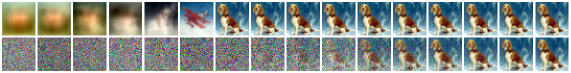
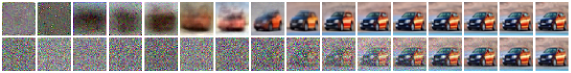
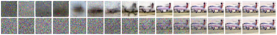
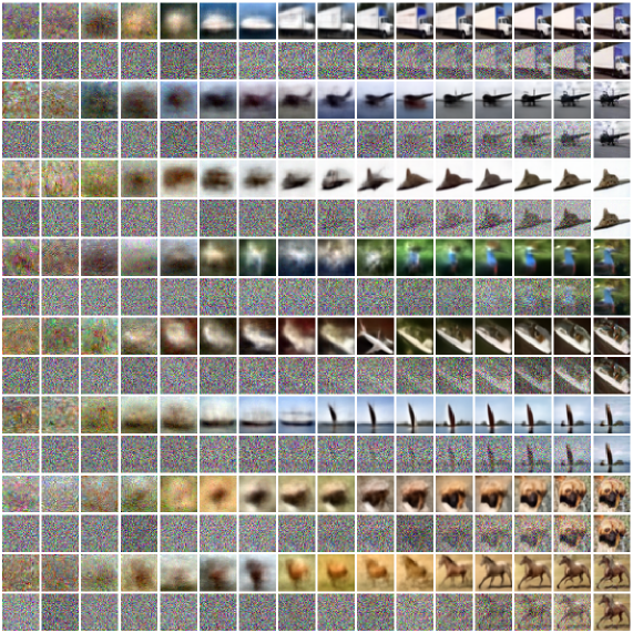
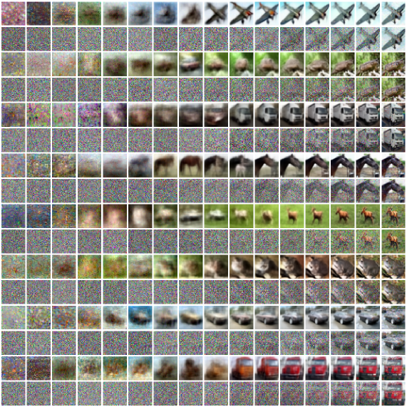
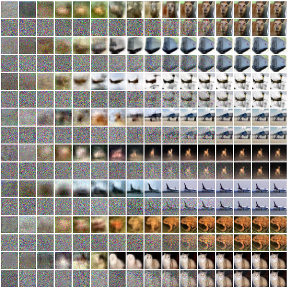
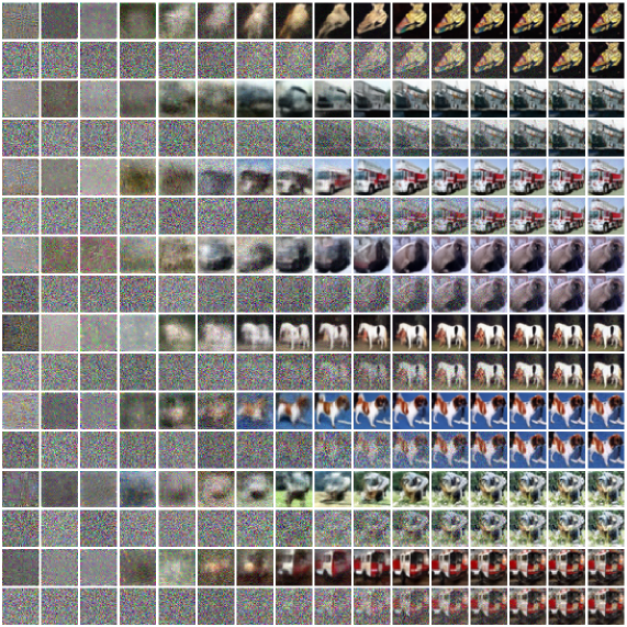
The expectations are convex linear combinations of the samples from . Explicitly, , where the weights are the probabilities, under the distributions (time-reversal sampling process 3) and (mixture of diffusions process from Section 3.2), of reaching each state at terminal time from at time . By construction, the initial weights entering expectation 20 are all equal to when starts from a fixed value , and are so on average when is stochastic. The initial weights entering expectation 21 are on average approximately equal to , depending on the quality of the approximation . Thus, is an averaging of many samples . As time progresses, changes in correspond to changes in through changes in the weights . Eventually all mass concentrates on a single weight corresponding to a dataset sample . Ultimately, the attractor dynamics implied by drive to . We provide an inspection in Figure 1, where stands for the training portion of the CIFAR10 dataset, and Euler(T) corresponds to the Euler scheme (Kloeden & Platen, 1992) applied with T discretization steps.
In the VESDE and VPSDE of Song et al. (2021) we have and reversing 21 gives
| (22) |
where is the true score. We can thus take a trained score model , plug it in 22, and verity the extent to which has been approximated, see Figure 1.

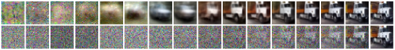
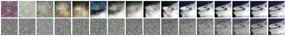
We pause for a moment to review the findings of Figure 1 (see Appendix D for additional related plots). Firstly, we can classify the dynamics of and of the associated weights in three stages. In the \nth1 stage the weights do not move much. During the \nth2 stage, roughly , the weights’ mass gets distributed over a limited number of samples. Interestingly, the weights’ dynamics are not monotonic. As time progresses the weights’ mass shifts between different objects from different classes. From the beginning of the \nth3 stage all mass gets allocated to a single weight, the terminal image is decided well in advance of the terminal time. These dynamics are suboptimal. We would like to shorten the \nth1 stage, but it is associated with large values of (i.e. quick time passing) which are required to decouple from . This is an intrinsic limitation of time-reversal approaches. It is also dubious that (partially) sampling multiple objects over is beneficial for efficient generative modeling when we make use only of the terminal sample. This issue applies to trained models as well, as the \nth3 row of Figure 1 shows. An interesting open question is how to obtain more suitable dynamics, where perhaps class transitions happen rarely. Secondly, provides a denoised representation of across the whole \nth3 stage. An alternative to the noise removal step applied to in Song et al. (2021) is to consider as the sampling process instead. Thirdly, Figure 1 makes it clear that lowering the number of discretization steps affects generative sampling in multiple ways. On the one hand the terminal sample is more noisy. This is not very surprising: close to the drift adjustment is approximately , which is the drift of a Brownian bridge. Bridge sampling is notoriously problematic (Bladt et al., 2016). On the other hand larger discretization errors also significantly affect the dynamics of resulting in less coherent samples. We remark that none of these insights could have been gained by observing alone, i.e. the even cells’ rows of Figure 1. To conclude, 20 and 21 give an additional meaning to “denoising”. Neural network approximators need to map from a noisy input to an adjustment toward a smoother superimposition of samples. The desire to minimize the discrepancy between the smoothness properties of and that of motivates the developments of Section 8.
6 Transports Approximation
As in Song et al. (2021), computing the multiplicative drift adjustment requires operations. In this Section we introduce three training objectives for which unbiased and scalable, i.e. with respect to , MC estimators can be immediately derived.
The first training objective applies only to . It relies on the identity (Appendix A)
| (23) |
It is advantageous to consider the right-hand side of 23 because from 8 we know that has mixture representation. As in Song et al. (2021), we can rely on Vincent (2011) to obtain a scalable objective to train a neural network approximator , i.e.
| (24) |
where is a regularization term.
The remaining training objectives rely on the identities 20 and 21. The goal is directly approximate the expectations of 20 and 21 which, as in Section 5, we denote with a generic . That is, we aim to train a neural network approximator . As conditional expectations are mean squared error minimizers, suitable objectives for the expectation terms of 20 and 21 are
| (25) | |||
| (26) |
In Table 1 we summarize the operations needed to implement the plain MC estimators for the four objectives considered in this work. We reference where to find the required quantities for SDEs 11 and 12. The MC estimators for the Fisher divergence losses involve multiplications by (by 15 and 17). Moreover, computing the drift adjustment at generation time requires multiplications by . In Section 8 we discuss how to manage the computational burden. An appealing property of is that computing the drift adjustment only requires the application of simple scalar functions (see 20 and 21), and that their MC estimators only requires sampling operations. A further advantage of is that no regularization is required. In contrast, in the absence of regularization terms, are divergent for due to the term (Section 5).
7 DBMT Overview and Numerical Experiment
In this section we finalize the DBMT construction, putting together the results of Sections 3, 4 and 6. The unconstrained SDE follows 11 or 12. It remains to choose the mixing distribution . The marginal needs to match , but there is flexibility in the choice of . Song et al. (2021) derived a random ordinary differential equation (RODE) matching the marginal distribution of a generative SDE, leading to faster sampling and to likelihood evaluation. RODE-matching requires to have density. A natural implementation is given by the factorial distribution with and the unconstrained SDE following 12 with which preserves . If instead the DBMT starts from a fixed value , i.e. , we can choose to remove the drift adjustment at (see 20) and reduce the work required to transport to . Finally, the use of non-factorial distributions can lead to a more efficient implementation, by linking the initial distribution to .
The training steps for the simplest objective 25 of Section 6 are reported in Algorithm 1. Batch size is assumed to be 1 to ease the description. It is also assumed that is factorial, otherwise the obvious modification applies to line 2 (Algorithm 2 is unaffected) where the endpoints are sampled. At line 3 a random central time and the corresponding state are sampled. The function optimizationstep implements a step of stochastic gradient descent update based on the loss . The corresponding sampling algorithm is reported in Algorithm 2 where the Euler(T) discretization is assumed in line 6. , , , are defined in Section 4. Section 8 shows how to sample efficiently from and in computer vision applications.
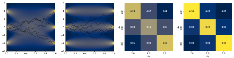
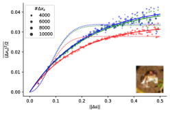
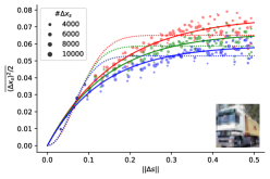
We consider a toy numerical example with , . The unconstrained SDE follows the standard Brownian motion. We consider two mixing distributions: independent mixing where and are independent and fully dependent mixing where . The results are reported in Figure 2. For both couplings the correct terminal distribution is recovered, as can be seen by taking the row-wise sum of the transition matrices. The initial-terminal distribution of solving 8, which realizes the DBMT, is different from the corresponding mixing distribution which is realized by the mixture process . results in a transition matrix of equal entries , results in a diagonal transition matrix of equal diagonal entries .
8 Non-Denoising Diffusions
In computer vision applications, images of resolution corresponds to . The use of an arbitrary covariance matrix in 11 and 12 requires its Cholesky (or equivalent) decomposition with cost . As the resolution increases the computational burden gets intractable very quickly. Indeed, to the best of the authors’ knowledge, all prior DDPM literature only considers independent transitions, that is . We suggest to view SDEs 11 and 12 as corresponding to the space discretization on an grid of a spatio-temporal process defined over the spatial domain . Consider the Euler discretization of 12: , where , the idea is to adopt a functional perspective: where defines space coordinates. That is, both and at each time are random processes over . We assume the innovations to be a Gaussian process (GP) for each .
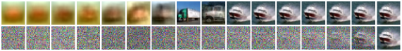
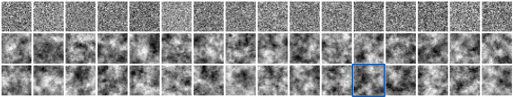
As the GPs are defined on a 2D domain we can leverage on scalable inference techniques from spatial statistics. As an example, we consider the circulant embedding method (CEM) (Wood & Chan, 1994; Dietrich & Newsam, 1997) which exploits a connection with the fast Fourier transform (FFT). See Appendix C for a cursory review of the CEM. Consider an uniform grid of size discretizing , i.e. the support of images. For a stationary covariance function the CEM samples on with cost . This is close to the cost of sampling from a pure white-noise process, and compares very favorably to the cost of a Cholesky decomposition. One limitation of CEM is that generated samples, while always Gaussian, might not have the correct covariances. Whether this happens, and in that case the quality of the approximation, depends on the covariance function. In Appendix C we select and fit an isotropic GP to the microscale properties of . For this estimated GP sampling is exact. Figure 3 shows samples from a pure white-noise GP, i.e. , (\nth1 row) and from the fitted GP using CEM (\nth2 row). As noted in Section 6, sampling is enough to implement the MC estimators for , but the MC estimators and drift adjustments for involve additional matrix multiplications by and . The CEM allows to compute these at the same cost if we define the GP on a 2D torus (Rue & Held, 2005, Chapter 2.1). This corresponds to introducing dependencies between “opposing” boundaries of . Figure 3 (\nth3 row) shows some samples, in the highlighted patch the opposing-boundaries dependency is evident. Either way, all samples from the \nth2 and \nth3 rows of Figure 3 match the smoothness properties of .
9 Conclusions
The DBMT construction of Section 3 is exact. The SDE class of Section 4 is tractable as it results in linear diffusion bridges. The time-space factorization of the diffusion coefficient separates modeling concerns: corresponds to a time-wrapping, can be efficiently modeled by fitting the microscale properties of . Availability of GPU-accelerated FFT implementations motivates our focus on the CEM. Alternative scalable approaches abound, from Gaussian Markov Random Fields (Rue & Tjelmeland, 2002; Rue, 2001) to Karhunen–Loève expansions (Betz et al., 2014). It remains to apply the results of this work to perform an empirical benchmarking. Section 6 develops three novel training objectives, two of which with desirable properties compared to the objective of Song et al. (2021), especially for non-factorial transitions. We remark the simplicity of the proposed DBMT approach (Algorithms 1 and 2) compared to alternatives grounded in the Schrödinger bridge problem (De Bortoli et al., 2021; Wang et al., 2021; Vargas et al., 2021). The understanding of the target mappings (21 and 20) can guide the development of neural networks more closely matching the target structure compared to the U-Net default choice. https://github.com/? links to the code accompanying this paper which is made available under the MIT license.
References
- Anderson (1982) Brian D.O. Anderson. Reverse-Time Diffusion Equation Models. Stochastic Processes and their Applications, 12(3):313–326, May 1982.
- Betz et al. (2014) Wolfgang Betz, Iason Papaioannou, and Daniel Straub. Numerical Methods for the Discretization of Random Fields by Means of the Karhunen–Loève Expansion. Computer Methods in Applied Mechanics and Engineering, 271:109–129, April 2014.
- Bladt et al. (2016) Mogens Bladt, Samuel Finch, and Michael Sørensen. Simulation of Multivariate Diffusion Bridges. Journal of the Royal Statistical Society. Series B (Statistical Methodology), 78(2):343–369, 2016.
- Brigo (2002) Damiano Brigo. The General Mixture-Diffusion SDE and Its Relationship with an Uncertain-Volatility Option Model with Volatility-Asset Decorrelation, December 2002.
- Cressie (1993) Noel Cressie. Statistics for Spatial Data. John Wiley & Sons, 1993.
- De Bortoli et al. (2021) Valentin De Bortoli, James Thornton, Jeremy Heng, and Arnaud Doucet. Diffusion Schrödinger Bridge with Applications to Score-Based Generative Modeling, June 2021.
- Dietrich & Newsam (1997) C. R. Dietrich and G. N. Newsam. Fast and Exact Simulation of Stationary Gaussian Processes through Circulant Embedding of the Covariance Matrix. SIAM Journal on Scientific Computing, 18(4):1088–1107, July 1997.
- Haussmann & Pardoux (1986) U. G. Haussmann and E. Pardoux. Time Reversal of Diffusions. The Annals of Probability, 14(4):1188–1205, October 1986.
- Ho et al. (2020) Jonathan Ho, Ajay Jain, and Pieter Abbeel. Denoising Diffusion Probabilistic Models. In H. Larochelle, M. Ranzato, R. Hadsell, M. F. Balcan, and H. Lin (eds.), Advances in Neural Information Processing Systems, volume 33, pp. 6840–6851, 2020.
- Karatzas & Shreve (1996) Ioannis Karatzas and Steven E. Shreve. Brownian Motion and Stochastic Calculus. Number 113 in Graduate Texts in Mathematics. Springer, New York, 2nd ed edition, 1996. ISBN 978-0-387-97655-6 978-3-540-97655-4.
- Kloeden & Platen (1992) Peter E. Kloeden and Eckhard Platen. Numerical Solution of Stochastic Differential Equations. Springer Berlin Heidelberg, Berlin, Heidelberg, 1992. ISBN 978-3-642-08107-1 978-3-662-12616-5.
- Krylov (1995) NV Krylov. Introduction to the Theory of Diffusion Processes, volume 142. Providence, 1995.
- Millet et al. (1989) Annie Millet, David Nualart, and Marta Sanz. Integration by Parts and Time Reversal for Diffusion Processes. The Annals of Probability, pp. 208–238, 1989.
- Rogers & Williams (2000) L Chris G Rogers and David Williams. Diffusions, Markov Processes and Martingales: Volume 2: Itô Calculus, volume 2. Cambridge university press, 2000.
- Rue (2001) Havard Rue. Fast Sampling of Gaussian Markov Random Fields. Journal of the Royal Statistical Society. Series B (Statistical Methodology), 63(2):325–338, 2001.
- Rue & Held (2005) Håvard Rue and Leonhard Held. Gaussian Markov Random Fields: Theory and Applications. Number 104 in Monographs on Statistics and Applied Probability. Chapman & Hall/CRC, Boca Raton, 2005. ISBN 978-1-58488-432-3.
- Rue & Tjelmeland (2002) Hååvard Rue and Hååkon Tjelmeland. Fitting Gaussian Markov Random Fields to Gaussian Fields. Scandinavian Journal of Statistics, 29(1):31–49, 2002.
- Sohl-Dickstein et al. (2015) Jascha Sohl-Dickstein, Eric Weiss, Niru Maheswaranathan, and Surya Ganguli. Deep Unsupervised Learning using Nonequilibrium Thermodynamics. In Proceedings of the 32nd International Conference on Machine Learning, volume 37 of Proceedings of Machine Learning Research, pp. 2256–2265. PMLR, 2015.
- Song et al. (2021) Yang Song, Jascha Sohl-Dickstein, Diederik P Kingma, Abhishek Kumar, Stefano Ermon, and Ben Poole. Score-Based Generative Modeling through Stochastic Differential Equations. In International Conference on Learning Representations, 2021.
- Särkkä & Solin (2019) Simo Särkkä and Arno Solin. Applied Stochastic Differential Equations. Cambridge University Press, first edition, April 2019. ISBN 978-1-108-18673-5 978-1-316-51008-7 978-1-316-64946-6.
- Vargas et al. (2021) Francisco Vargas, Pierre Thodoroff, Austen Lamacraft, and Neil Lawrence. Solving Schrödinger Bridges via Maximum Likelihood. Entropy, 23(9):1134, September 2021.
- Vincent (2011) Pascal Vincent. A Connection Between Score Matching and Denoising Autoencoders. Neural Computation, 23(7):1661–1674, July 2011.
- Wang et al. (2021) Gefei Wang, Yuling Jiao, Qian Xu, Yang Wang, and Can Yang. Deep Generative Learning via Schrödinger Bridge, June 2021.
- Wood & Chan (1994) Andrew T. A. Wood and Grace Chan. Simulation of Stationary Gaussian Processes in [0,1]d. Journal of Computational and Graphical Statistics, 3(4):409–432, 1994.
- Øksendal (2003) B. K. Øksendal. Stochastic Differential Equations: An Introduction with Applications. Universitext. Springer, Berlin ; New York, 6th ed. edition, 2003. ISBN 978-3-540-04758-2.
Appendix A Theoretical Framework
A.1 Assumptions
Assumption 1 (SDE solution).
A given -dimensional SDE with associated initial distribution and integration interval admits a unique strong solution on .
Assumption 1 can be checked through the application of the standard existence and uniqueness theorems for SDE solutions. Of particular relevance to our setting is the formulation of Krylov (1995, Chapter 5, Theorem 1) that limits the monotonic requirement to, informally speaking, drifts that pull the process toward infinities.
Assumption 2 (SDE density).
A given -dimensional SDE with associated initial distribution and integration interval admits a marginal / transition density on with respect to the -dimensional Lebesgue measure that uniquely satisfies the Fokker-Plank / Kolmogorov-forward partial differential equation (PDE).
We refer to Särkkä & Solin (2019, Chapter 5) and to Karatzas & Shreve (1996, Chapter 5.7) for connections between SDEs and PDEs.
All theoretical results of this work rely on simple algebraic manipulations and re-arrangements of quantities of interest. The main complication stems from the need to justify differentiation and integration exchanges, i.e. exchange of limits.
Assumption 3 (exchange of limits).
We assume that limits exchanges are justified in the steps marked with and .
Similarly, various steps in the derivations involve considering fractional quantities with densities appearing in the denominators.
Assumption 4 (positivity).
For a given stochastic process, all finite-dimensional densities, conditional or not, are strictly positive.
Assumption 4 is easy to verify. We resorted to the practical but somewhat unsatisfactory formulation of Assumption 3 because in full generality it is complicated to give easy to check conditions. We just note that when , the limit exchange marked with is always justified. So are the limits exchanges marked with when in addition puts all the mass to a fixed initial value, or (by direct verification) when is Gaussian for the SDE class of Section 4. Thorough this paper, both in the main text and in the proofs that follow, it is supposed that Assumptions 1, 2 and 4 are satisfied by SDEs 1, 6 and 7. This is the case for the SDE class of Section 4, i.e. 11 and 12, for any with finite variance.
Remark: For ease of exposition it is assumed thorough this paper that all diffusions take values in the state space . There is no impediment in extending the presented results to the case of diffusions taking values in a subset . The obvious changes to Assumptions 1, 2, 3 and 4 apply, the proofs carry over without substantial modifications. This extension could be of practical interest as images are often represented as floating point values in .
A.2 Statement and Proof of Diffusion Mixture Representation Theorem
Theorem 2 (Diffusion mixture representation).
Consider the family of -dimensional SDEs on indexed by
| (27) | ||||
where the initial distributions and the BMs are all independent. Let denote the marginal density of . For a generic mixing distribution on , define the mixture marginal density for and the mixture initial distribution by
| (28) |
Consider the -dimensional SDE on defined by
| (29) | ||||
It is assumed that all diffusion processes and the diffusion process solving 29 satisfy the regularity assumptions Assumptions 1, 2 and 4 and that Assumption 3 holds. Then the marginal distribution of the diffusion is .
Proof of Theorem 2.
We start by establishing that the law of is indeed given by the solution of 29. In this proof we make use of the following notation: for scalar-valued , for vector-valued , for matrix-valued . This notation allows for a compact representation of PDEs reminiscent of the 1-dimensional setting. Then, for we have that
| () | |||
| () |
The second line is an exchange of limits, the third line is the application of the Fokker-Plank PDEs for the collection of processes , the fourth line is a rewriting in terms of , the last line is another exchange of limits. The result follows by noticing that the last line gives the Fokker-Plank representation of 29. ∎
A.3 Drift Adjustments
Limitedly to this section, we lighten the notation by removing subscripts from probability measures and densities. The missing time points can be inferred without ambiguity from the variables.
A.3.1 Drift Adjustment Identities for Constant Initial Value
First identity:
| () | |||
Second identity:
A.3.2 Drift Adjustments as Expectations
Appendix B SDEs Class Formulas
The transition densities of 9 and 10 are given respectively by
Here we used the notation , i.e. is the average value of a function on the interval . The time-homogenous case of 10, where , is thus immediately recovered.
The scalar functions , , and are given by
The scalar functions , and are given by
The scalar functions and are given by
The constants depend in part on the dataset considered, but are consistently chosen to have small for and large for .
The approximating distributions in Song et al. (2021) are for VESDE, for VPSDE.
Appendix C Additional Material
C.1 Closely Related Work
A work closely related to the present paper is that of Wang et al. (2021) as it similarly avoids the time-reversal construction. Wang et al. (2021) construct a 2-stages diffusion process from a constant initial value to by relying on the theory of Schrödinger bridges. The most notable differences with respect to the DBMT transport are: (i) the dynamics considered in Wang et al. (2021) are less general, in our notation they correspond to for a fixed scalar ; (ii) the transport proposed in Wang et al. (2021) necessarily starts from , the general result of 8 allows for (almost) arbitrary initial distributions and initial-terminal dependencies. For an initial , i.e. for case of in Section 3.2 and for the more limited dynamics considered in Wang et al. (2021), the achieved transport is the same. In this sense the DBMT generalizes the first stage diffusion of Wang et al. (2021). It is interesting to note that in the case of a constant the DBMT can also be obtained by an application of Doob -transforms as we show in the following section.
We now review two additional works grounded in the Schrödinger bridge problem: De Bortoli et al. (2021); Vargas et al. (2021). Both works rely on the Iterative Proportional Fitting (IPF) procedure to solve the (dynamic) Schrödinger bridge problem. Both works leverage on time-reversal results to carry out the alternated Schrödinger half-bridge IPF iterations. The main difference between the two works is that De Bortoli et al. (2021) estimates the optimal SDE drifts via neural network approximations and score-matching, while Vargas et al. (2021) relies on Gaussian Processes and maximum likelihood fitting. The work of De Bortoli et al. (2021) can be seen as an extension of Song et al. (2021), and similarly to our work allows the use of shorter time intervals. Compared to our proposal, it solves a harder problem but also presents additional difficulties. Training is more involved as all the neural network approximations, one for each IPF iterate, need to converge. Moreover, there is limited guidance on how to optimally choose the number of integration steps over the number of IPF iterates.
C.2 Connection with Doob h-transforms
The previously established identity
shows that the drift adjustment can be equivalently expressed as
as is a constant. It can be verified that the function satisfies the required space-time regularity property (Särkkä & Solin, 2019, Eq. (7.73)). As such, it is a genuine Doob -transform. That is the transition density of the DBMT transport from to follows by direct computation.
C.3 GP Modelling on CIFAR10
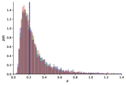
For simplicity, we assume a factorial distribution over the channels and an isotopic stationary covariance function. We rely on the semivariogram approach (Cressie, 1993) to compare how different covariance functions fit . A semivariogram is a measure of dependency across space. In the case of an isotropic stationary covariance it simplifies to a scalar function of the Euclidean distance between points: with . The rate of decrease of toward as gives a measure of the infinitesimal spatial dependency, i.e. the smoothness of the spatial process. Semivariograms corresponding to different covariance functions are here fitted to their empirical counterparts via a weighted minimum-least-squares procedure (Cressie, 1993). Figure 4 illustrates the exponential and RBF semivariogram fits for two images of . The exponential covariance, which corresponds to rougher paths, provides a much better fit to the shown samples. This result is consistent across . We remark that corresponds to a pure white-noise process with a perfectly flat semivariogram which would clearly result in a very poor fit to the empirical semivariograms shown in Figure 4. Based on these findings, we model the innovations of each image channel as a GP with exponential covariance function with length-scale , the median estimated value (Figure 4 (right)). We match the marginal variance to that of , .
C.4 Circulant Embedding Method
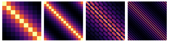
We start by providing a cursory explanation leading to efficient sampling in the 1D case, before giving the intuition behind the extension to the 2D case. We refer to Wood & Chan (1994); Dietrich & Newsam (1997) for a complete explanation and to Rue & Held (2005) for the results underlying efficient density (likelihood) computation. Let be the spatial domain of interest. Let be a uniform grid (regular lattice) discretizing , where the points are assumed to be ordered. The first key observation is that for a stationary covariance function the covariance matrix with entries is symmetric and Toeplitz, i.e. with constant-diagonals. See Figure 5 (leftmost) for an example where . A property of symmetric Toeplitz matrices is that they can always be embedded in larger symmetric circulant matrices. A circulant matrix of size is defined by the property that all its rows (and columns) are obtained by cycling through the same -dimensional vector. Circulant matrices correspond to covariance matrices of GPs defined on a (here 1D) torus (Rue & Held, 2005, Chapter 2.1). The circulant embedding matrix just introduced corresponds to an artificial enlargement of the spatial domain to a larger interval leading to a torus. See Figure 5 (\nth2 from left) for a circulant embedding of . The second key observation is that a circulant matrix is diagonalized by the 1D FFT matrix. Having obtained the eigenvalues of , efficient sampling on the enlarged domain is achieved by the 1D FFT applied to complex standard random numbers multiplied by the (square root of the) eigenvalues. The real and imaginary part of the generated samples are independent. The main issue with the CEM is that the circulant matrix embedding might fail to be positive definite. The issue can be avoided by considering progressively larger embeddings, see the theoretical and empirical findings of Dietrich & Newsam (1997). Otherwise, a level of approximation can be accepted by modifying the covariance function or by truncating the eigenvalues to be positive.
The development of the 2D CEM follows very similar steps. The domain of interest is now , the uniform grid is and the points are assumed to be lexicographically ordered. The stationarity of the covariance functions results in a symmetric block-Toeplitz covariance matrix, as shown in Figure 5 (\nth3 from left). Again, symmetric block-Toeplitz matrices can be embedded in symmetric block-circulant matrices, as exemplified by Figure 5 (rightmost, zooming might be required to see the block structure). Block-circulant matrices can be shown to be diagonalized by the 2D FFT matrix, and efficient sampling follows from similar steps to the ones seen in the 1D case.
Appendix D Additional Figures