Inference on the state process of periodically inhomogeneous hidden Markov models for animal behavior

Abstract

Over the last decade, hidden Markov models (HMMs) have become increasingly popular in statistical ecology, where they constitute natural tools for studying animal behavior based on complex sensor data. Corresponding analyses sometimes explicitly focus on — and in any case need to take into account — periodic variation, for example by quantifying the activity distribution over the daily cycle or seasonal variation such as migratory behavior. For HMMs including periodic components, we establish important mathematical properties that allow for comprehensive statistical inference related to periodic variation, thereby also providing guidance for model building and model checking. Specifically, we derive the periodically varying unconditional state distribution as well as the time-varying and overall state dwell-time distributions — all of which are of key interest when the inferential focus lies on the dynamics of the state process. We use the associated novel inference and model-checking tools to investigate changes in the diel activity patterns of fruit flies in response to changing light conditions.

Keywords: Markov chain, seasonality, sojourn time, stationary distribution, statistical ecology, time series

1 Introduction

1.1 Inference on periodic variation in animal behavior

Over the last two decades, advances in biologging technology have revolutionized behavioral ecology (Hussey et al.,, 2015; Kays et al.,, 2015). Complex sensor data, nowadays often collected at very high resolution (e.g. 1 Hz), allow ecologists to more precisely identify foraging and other movement maneuvers employed by animals, to reveal their interaction with conspecifics and prey, and ultimately to infer how they cope with environmental and anthropogenic change (Nathan et al.,, 2022). In particular, driven by these technological advancements, periodic variation in animal behavior can now be studied under natural conditions. This allows for comprehensive inference focused, for example, on the identification of diurnal rhythms, the quantification of individual heterogeneity in diel variation, and the prediction of seasonal patterns or events such as migratory behavior (Hertel et al.,, 2017; Weegman et al.,, 2017; Jannetti et al.,, 2019; Beumer et al.,, 2020). Even if not of primary interest, ignoring such periodic variation can invalidate statistical inference: standard errors might be underestimated due to residual autocorrelation, and the model formulation as guided by information criteria may be more complex than necessary to compensate for the model misspecification (Li and Bolker,, 2017; Pohle et al.,, 2017).

A statistical framework that naturally lends itself to inference on the dynamics of animal behavior in general, and periodic variation therein in particular, is given by the class of hidden Markov models (HMMs). In HMMs, the movement metrics observed — for instance, the step lengths and turning angles between successive GPS fixes, or the dynamic body acceleration calculated from acceleration sensors — are regarded as noisy measurements of the underlying, serially correlated behavioral process of the animal (Langrock et al.,, 2012; Leos-Barajas et al.,, 2017; McClintock et al.,, 2020). Ecological inference then mostly focuses on this unobserved behavioral state process, typically modeled as a finite-state Markov chain. To account for periodic variation in animal behavior, the state-switching probabilities are commonly modeled as functions of time, for example by specifying trigonometric base functions with the desired wavelength as covariates using a multinomial logistic regression framework (Li and Bolker,, 2017; Patterson et al.,, 2017; Feldmann et al.,, 2023).

For time-homogeneous Markov chains, implications of the estimated state-switching probabilities for behavioral time budgets can conveniently be characterized by (i) the stationary distribution, that is the unconditional distribution of the states, and (ii) the state dwell-time distributions. Regarding (i), when including periodic effects in the state process, inference on temporal variation in state occupancy is hampered by the fact that an inhomogeneous Markov chain does not have a stationary distribution. Instead, an approximate version has commonly been reported in the literature (Farhadinia et al.,, 2020; Byrnes et al.,, 2021), which in general is biased as it ignores the inhomogeneous evolution of the state process. Regarding (ii), as a consequence of the Markov property, the state dwell times in homogeneous HMMs are geometrically distributed, implying that the most likely duration of a stay within a state is one time unit, which is often biologically unrealistic. Inhomogeneity in the state process, and in particular temporal variation, does however affect the dwell-time distributions — yet to what extent this may alleviate the potentially undesirable characteristics of homogeneous Markov state processes has not been investigated.

In this contribution, we analytically derive the main properties of periodically inhomogeneous Markov state processes, namely (i) the time-varying unconditional distribution of the states and (ii) the state dwell-time distribution (both overall and at fixed times). Regarding (i), we demonstrate that the approximate state distribution frequently used as an important summary output in analyses of ecological systems can in fact be severely biased. Regarding (ii), we find that the state dwell-time distributions implied by HMMs with periodic components can deviate substantially from a geometric distribution. This highlights that temporal covariates may to some extent compensate for biologically unrealistic consequences of the Markov property. Our results do in fact apply to periodically inhomogeneous Markov chains in general — i.e. not only to those that form the state process within an HMM — but we focus on their role specifically within ecological applications of HMMs, as our research is motivated by the study of temporal niche mechanisms and, more generally, periodic variation in animal behavior, as inferred from noisy sensor data.

1.2 Motivating data

We aim to study the influence of external conditions on the behavior of common fruit flies (Drosophila melanogaster) and especially their circadian clock. Like the majority of animal species, fruit flies restrict their behavioral activity to specific time periods during the 24-hour cycle, a mechanism referred to as the temporal niche. In particular, synchronizing their circadian clocks to the common light-dark (LD) cycles improves the flies’ fitness as they anticipate daily environmental changes (Beaver et al.,, 2002; Bernhardt et al.,, 2020). To investigate these diel activity patterns, 15 male wild-type fruit flies aged two to three days were trained under a standard lighting schedule of twelve hours of light followed by twelve hours of darkness (LD condition) for four days. Subsequently, the flies were exposed to six consecutive days of uninterrupted darkness (DD condition). They were kept in special tubes that tracked their locomotor activity by counting each time a fly passed an infrared beam in the middle of the tube. We aggregated these counts into half-hour bins, leading to a total of 6840 observations ranging from 0-300. Boxplots of the activity counts for the different times of day, separated into LD and DD conditions, are shown in Figure 1. The strong diel activity pattern emerges from the flies’ anticipation of the light transitions in the morning and evening in the LD condition. In constant darkness, the bimodality is much less pronounced as the flies lose these reference points. We aim to precisely quantify such behavioral differences between the two light conditions, in particular comprehensively studying the state-switching dynamics leading to the bimodal activity pattern.

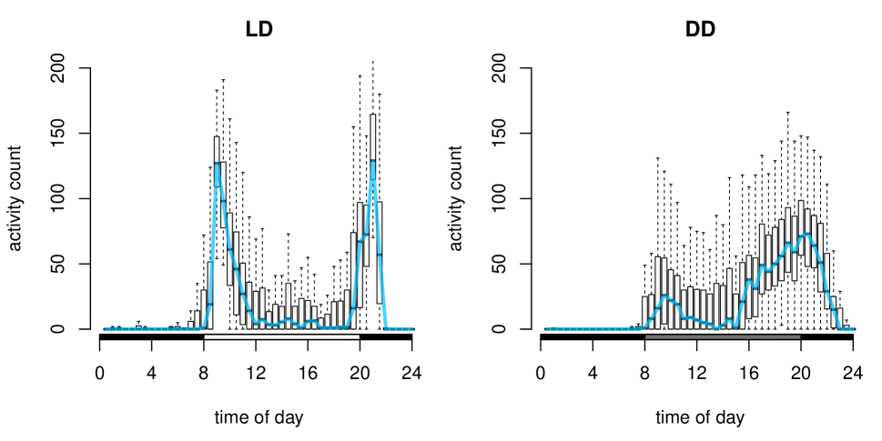
Figure 1: Boxplots of activity counts for each half-hour bin, including all individuals and all days but separated into LD and DD conditions. The thick blue line represents the median activity for visual clarity.

2 Methods

2.1 Hidden Markov models — definition and notation

We consider an HMM comprising a state-dependent process $\{X_{t}\}_{t\in\mathbb{N}}$ (where $X_{t}$ can be a vector) and a latent state process $\{S_{t}\}_{t\in\mathbb{N}}$, with $S_{t}\in\{1,\ldots,N\}$ selecting which of $N$ possible component distributions generates $X_{t}$. The state process $\{S_{t}\}$ is assumed to be a Markov chain of first order, characterized by its initial state distribution and the time-varying transition probability matrix (t.p.m.)

$$\bm{\Gamma}^{(t)}=(\gamma_{ij}^{(t)}),\;\text{ with }\;\gamma_{ij}^{(t)}=\Pr(S_{t+1}=j|S_{t}=i),\quad t\in\mathbb{N}.$$

The observed variables $X_{t}$, $t\in\mathbb{N}$, are assumed to be conditionally independent of each other, given the states.

The methodological development of this contribution is generally applicable but was motivated by ecological applications, where $S_{t}$ could for example indicate the animal’s behavioral state at time $t$ (e.g. resting, foraging, traveling), with $X_{t}$ some noisy measurement of that state (e.g. acceleration, movement speed, tortuosity of movement, as commonly recorded by biologgers). In these settings it is often necessary to incorporate periodic variation in the state-switching process, for example to account for diurnal rhythms. Associated models and their properties are discussed in the following two sections.

2.2 Time-varying state distribution in periodically inhomogeneous Markov state processes

We consider a setting with periodically varying state-switching dynamics, such that

$$\bm{\Gamma}^{(t)}=\bm{\Gamma}^{(t+L)}$$ (1)

for $t\in\mathbb{N}$, with $L$ denoting the length of a cycle. For ease of notation, we restrict the index $t$ to $\{1,\dotsc,L\}$ corresponding to the $L$ unique matrices.

For hourly data and $N=2$, we could for example model time-of-day variation ($L=24$) as

$$\text{logit}\bigl{(}\gamma_{ij}^{(t)}\bigr{)}=\beta_{0}^{(ij)}+\beta_{1}^{(ij)}\sin\Bigl{(}\frac{2\pi t}{24}\Bigr{)}+\beta_{2}^{(ij)}\cos\Bigl{(}\frac{2\pi t}{24}\Bigr{)},\;\text{ for }i\neq j.$$ (2)

The interpretation of such transition probabilities as functions of time can be tedious, especially when $N>2$. Therefore, it has become common practice to instead consider a summary statistic, namely the periodically varying (unconditional) distribution of the states. This distribution is usually approximated by the hypothetical stationary distribution that would emerge if the process followed transition dynamics specified by holding $\bm{\Gamma}^{(t)}$ constant over time (for given $t$), i.e.  the solution to $\bm{\rho}^{(t)}=\bm{\rho}^{(t)}\bm{\Gamma}^{(t)}$ for each $t=1,\ldots,L$, subject to $\sum_{i=1}^{N}\rho_{i}^{(t)}=1$ (Patterson et al.,, 2009). The approximation will in general be biased because it ignores the preceding process dynamics as implied by $\bm{\Gamma}^{(t-1)},\bm{\Gamma}^{(t-2)},\ldots,\bm{\Gamma}^{(t-L)},$ and instead pretends that the process has been following the dynamics as implied by a constant $\bm{\Gamma}^{(t)}$ for a considerable time.

However, for periodically inhomogeneous Markov chains as defined in Equation (1), there is in fact no need for such an approximation. To see this, consider for fixed $t$ the thinned Markov chain $\{S_{t+kL}\}_{k\in\mathbb{N}}$, which is homogeneous with constant t.p.m.

$$\tilde{\bm{\Gamma}}_{t}=\bm{\Gamma}^{(t)}\bm{\Gamma}^{(t+1)}\ldots\bm{\Gamma}^{(t+L-1)}.$$

Visual intuition for the homogeneity of $\tilde{\Gamma}_{t}$ is given in Figure 2.

Provided that this thinned Markov chain is irreducible, it has a unique stationary distribution $\bm{\delta}^{(t)}$, which is the solution to

$$\bm{\delta}^{(t)}=\bm{\delta}^{(t)}\tilde{\bm{\Gamma}}_{t}$$ (3)

(Ge et al.,, 2006; Kargapolova and Ogorodnikov,, 2012; Touron,, 2019). For large $N$ or large $L$, it will typically be most convenient to calculate $\bm{\delta}^{(t)}$ recursively for $t=1,\ldots,L$ (see Appendix A.1). Assuming that the Markov chain starts in its stationary distribution, $\bm{\delta}^{(t)}$ is the state distribution at any time $t$ of interest, and we refer to such a process $\{S_{t}\}_{t\in\mathbb{N}}$ as a periodically stationary Markov chain. Otherwise, provided aperiodicity, the solution to Equation (3) will typically be a good approximation to the unconditional distribution of states, as each of the $L$ thinned Markov chains — i.e. $\{S_{t+kL}\}_{k\in\mathbb{N}}$ for $t=1,\ldots,L$ — converges to its respective stationary distribution $\bm{\delta}^{(t)}$. Therefore, we interchangeably use the terms (periodically) stationary distribution and unconditional state distribution.

Figure 2: Example visualization of periodic stationarity with $L=3$. The thinned Markov chain $S_{t},S_{t+3},S_{t+6},\dotsc$ has constant t.p.m. $\tilde{\bm{\Gamma}}^{(t)}$.

2.3 State dwell-time distribution of periodically inhomogeneous Markov chains

In this section we derive the distribution of the state dwell times implied by a periodically stationary Markov chain. We first focus on the time-varying state dwell-time distribution, i.e. the distribution of the duration of a stay in state $i$ beginning at time $t$, for each $t=1,\ldots,L$ and each $i=1,\ldots,N$.

Proposition 2.1.

Consider a periodically inhomogeneous Markov chain defined by $\bm{\Gamma}^{(t)}$, $t=1,\dotsc,L$. For this Markov chain, the probability mass function of the time-varying state dwell-time distribution of a stay in state $i$ beginning at time $t$ is

$$d_{i}^{(t)}(r)=\bigl{(}1-\gamma_{ii}^{(t+r-1)}\bigr{)}\prod_{j=1}^{r-1}\gamma_{ii}^{(t+j-1)},\quad r\in\mathbb{N}.$$ (4)

Equation (4) appears similar to the homogeneous case with geometric dwell-time distributions. However, in this case the transition probabilities evolve over time, and as a consequence the probability mass function of this dwell-time distribution is not necessarily monotonously decreasing (cf. Figure 6). A proof of Proposition 2.1 is given in Appendix A.2.

The time-varying state dwell-time distributions provide comprehensive information on the state dynamics within a cycle. However, visualization and interpretation of $L$ time-varying distributions for each state $i$ can be tedious (see Appendix A.3). As an alternative, the means of these distributions may provide a useful summary statistic.

Proposition 2.2.

In the setting of Proposition 2.1, let $R_{i}^{(t)}$ denote the dwell time in state $i$ beginning at time $t$. Then

$$\mathbb{E}R_{i}^{(t)}=\frac{L+\sum_{r=1}^{L}rd_{i}^{(t)}(r)}{\sum_{r=1}^{L}d_{i}^{(t)}(r)}-L.$$

A proof of this proposition is provided in Appendix A.2. Computing the expected dwell time for each state $i=1,\dotsc,N$ and each time point $t=1,\dotsc,L$, the variation in the mean dwell times over the course of a cycle can be concisely visualized (see Figure 3).

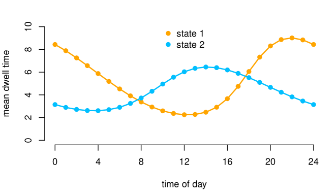
Figure 3: Means of the time-varying state dwell times of an example 2-state HMM with trigonometric modeling of periodic variation (see Appendix A.4 for the precise model configuration).

In practical applications, it may be cumbersome to interpret the time-varying dwell-time distributions, especially when the temporal resolution of the data is high (for example, with minute-by-minute data and diel variation, there would be $1440$ such distributions for each state). In addition, the focus of the inference with respect to state dynamics will often be on the overall distribution of the durations in the different states, not explicitly conditioning on the start time of the stay. We obtain such a distribution as a mixture of the time-varying dwell-time distributions.

Proposition 2.3.

For a periodically stationary Markov chain defined by $\bm{\Gamma}^{(t)}$, $t=1,\dotsc,L$, the probability mass function of the overall (unconditional) dwell-time distribution in state $i$ is

$$d_{i}(r)=\sum_{t=1}^{L}w_{i}^{(t)}d_{i}^{(t)}(r),\qquad r\in\mathbb{N},$$ (5)

with the mixture weights defined as

$$w_{i}^{(t)}=\frac{\sum_{l\in\mathcal{S}\setminus i}\delta_{l}^{(t-1)}\gamma_{li}^{(t-1)}}{\sum_{t=1}^{L}\sum_{l\in\mathcal{S}\setminus i}\delta_{l}^{(t-1)}\gamma_{li}^{(t-1)}},\quad t=1,\dotsc,L,$$

where $\mathcal{S}=\{1,\dotsc,N\}$, $\bm{\Gamma}^{(0)}=\bm{\Gamma}^{(L)}$, $\bm{\delta}^{(0)}=\bm{\delta}^{(L)}$ and $\bm{\delta}^{(t)}$ as in Equation (3). Letting $R_{i}$ denote the overall dwell time in state $i$, we further have that

$$\mathbb{E}R_{i}=\sum_{t=1}^{L}w_{i}^{(t)}\mathbb{E}R_{i}^{(t)}=\sum_{t=1}^{L}\left(w_{i}^{(t)}\frac{L+\sum_{r=1}^{L}rd_{i}^{(t)}(r)}{\sum_{r=1}^{L}d_{i}^{(t)}(r)}\right)-L.$$

The proof of Proposition 2.3 is given in Appendix A.2. For homogeneous Markov chains, i.e. when $\gamma_{ij}^{(t)}=\gamma_{ij}$ for all $t$ and all $i,j\in\mathcal{S}$, the state dwell-time distribution given in Equation (5) simplifies to the geometric case. To see this, we first note that

$$d_{i}^{(t)}(r)=\left(1-\gamma_{ii}^{(t+r-1)}\right)\prod_{j=1}^{r-1}\gamma_{ii}^{(t+j-1)}=(1-\gamma_{ii})\gamma_{ii}^{r-1}$$

is constant in time. Thus,

$$d_{i}(r)=\sum_{t=1}^{L}w_{i}^{(t)}(1-\gamma_{ii})\gamma_{ii}^{r-1}=(1-\gamma_{ii})\gamma_{ii}^{r-1}\sum_{t=1}^{L}w_{i}^{(t)}=(1-\gamma_{ii})\gamma_{ii}^{r-1},$$

as the sum of the weights $w_{i}^{(t)}$ equals one.

If, however, the Markov chain is not homogeneous, then the distribution in Equation (5) can deviate rather substantially from a geometric distribution, and may even be multimodal. To illustrate this, Figure 4 displays an example overall state dwell-time distribution implied by an HMM with trigonometric modeling of the periodic variation in the state transition probabilities (see Appendix A.4 for the model parameters leading to this outcome). To verify our theoretical results, we further complemented the exact probability mass function derived in Proposition 2.3 by an approximation using Monte Carlo simulations. While the latter can always easily be obtained, the exact theoretical result is of course advantageous with respect to both accuracy and computational cost.

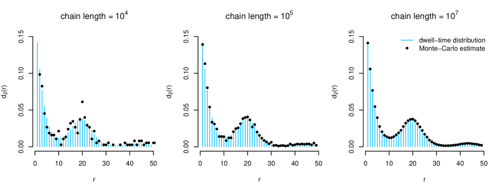
Figure 4: Overall state dwell-time distribution (state 2) of an example 2-state HMM with trigonometric modeling of periodic variation (see Appendix A.4 for the precise model configuration). Analytical distribution (blue bars) compared to Monte-Carlo-simulated state dwell times (black dots) for different chain lengths.

The time-varying and the overall state dwell-time distributions can provide valuable insights into the dynamics of the state process. In addition, these results can be used to devise comprehensive model-checking tools for HMMs with periodic variation. For example, the model-implied dwell-time distributions can be compared against the empirical state dwell times obtained from the Viterbi-decoded state sequence.

3 Application: Activity of Drosophila melanogaster

To investigate diel activity patterns in the motivating fruit fly data from Section 1.2, we model the half-hourly activity counts (cf. Figure 1) using a 2-state HMM with negative binomial state-dependent distributions, as was previously done in Feldmann et al., (2023). To allow for individual-specific differences in the flies’ activity levels, we model the state-dependent means as gamma-distributed random effects, while the dispersion parameters of the negative binomial distributions are fixed across individuals. The state transition probabilities are modeled as functions of the time of day, ensuring sufficient flexibility for capturing multiple activity peaks throughout the day via the use of trigonometric functions with wavelengths of 24, 12, and 8 hours, i.e.

$$\text{logit}\bigl{(}\gamma_{ij}^{(t)}\bigr{)}=\beta_{0}^{(ij)}+\sum_{k=1}^{3}\beta_{1k}^{(ij)}\sin\Bigl{(}\frac{2\pi kt}{48}\Bigr{)}+\sum_{k=1}^{3}\beta_{2k}^{(ij)}\cos\Bigl{(}\frac{2\pi kt}{48}\Bigr{)},\quad\text{ for }i\neq j.$$

As we are interested in behavioral differences between the lighting schedules, we estimate separate state-process parameters for the LD and DD conditions, respectively. To estimate the model parameters, we numerically maximize the joint likelihood computed as the product of the different individuals’ likelihoods. The random effects were marginalized out using numerical integration (Schliehe-Diecks et al.,, 2012). All models were implemented and fitted in R (R Core Team,, 2023) using a parallelized numerical optimization procedure (Gerber and Furrer,, 2019) to speed up the estimation.

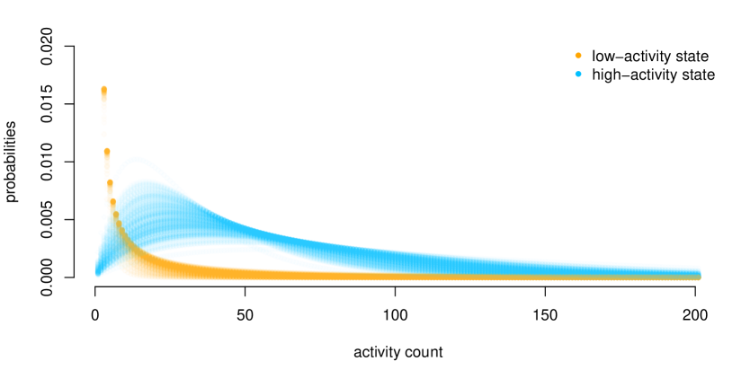
Figure 9: Weighted state-dependent distributions. 200 draws from the distribution of the random mean.

The fitted HMM distinguishes a low- and a high-activity state for all flies, while allowing for individual differences in their mean activity levels (cf. Figure 9 in the Appendix). To investigate the temporal variation in the state dynamics as well as the state dwell times, we apply the inferential tools developed in Section 2. The time-dependent unconditional state distributions as well as their approximations under the LD and the DD condition are shown in Figure 5. For both light conditions, the observed activity patterns (cf. Figure 1) are adequately reflected by the true stationary distribution of the inhomogeneous Markov chain, with the activity peaking shortly after the light transitions experienced by the flies in the LD setup. While the morning peak in activity is more pronounced under the LD condition, in constant darkness (DD) the flies are active for a longer period of time in the evening hours. In contrast to the true distribution $\bm{\delta}^{(t)}$, the high-activity peaks of the approximation $\bm{\rho}^{(t)}$ differ in shape and, more importantly, are shifted in time, falsely indicating activity to peak about 1-3 hours earlier (cf. also the empirical activity distribution shown in Figure 1). Therefore, the approximate version would inevitably result in erroneous conclusions when interested in the exact time and length of flies’ activity peaks.

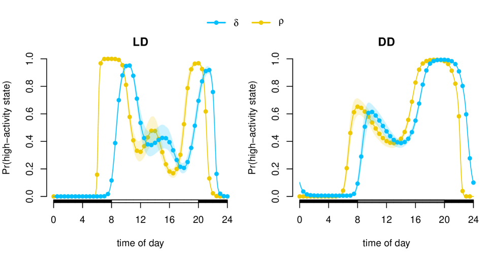
Figure 5: Periodic stationary distribution as a function of the time of day, for LD and DD condition. True stationary distribution (light blue) compared to biased approximation (yellow). Pointwise confidence intervals were obtained via Monte Carlo simulation from the approximate normal distribution of the maximum likelihood estimator.

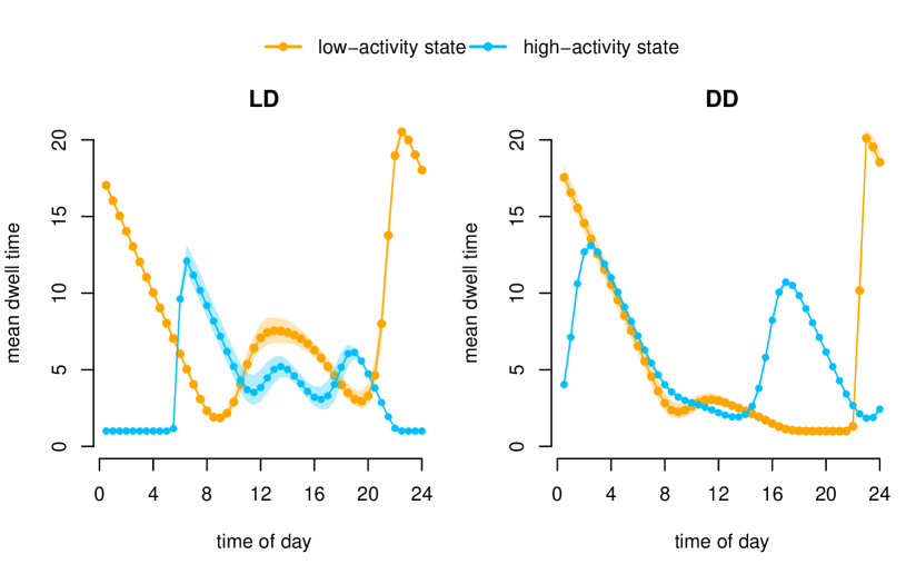
Figure 10: Mean dwell times as a function of the time of day, for LD and DD condition. Pointwise confidence intervals where obtained via Monte Carlo simulation from the approximate normal distribution of the maximum likelihood estimator.

To further characterize the state dynamics within a cycle, the time-varying dwell-time distributions as derived in Proposition 2.1 can provide temporally fine-grained insights. Due to the model accounting for periodic variation in the state-switching dynamics, the model-implied dwell times differ substantially from a geometric distribution, as illustrated in Figure 6. Specifically for the morning times when the light was just switched on, the distribution’s mode is clearly distinct from one — in other words, the flies’ response to the environmental change is not only to become active, but also to remain active for an extended period of time. During noon and in the early afternoon, activity bouts are more likely to be short. Overall, the time-varying dwell-time distributions thus reflect and complement the information gained from the stationary distribution (cf. Figure 5). However, since it is tedious and hardly feasible to look at all time-dependent dwell-time distributions for both states in the LD and DD condition ($48\times 2\times 2=192$ in total), it can be useful to instead plot the time-varying means of the distributions as derived in Proposition 2.2 (cf. Figure 10 in the Appendix). These mean dwell times summarize the distinct patterns of varying durations in the high- and low-activity state over a day and stress differences between both light conditions. Solely focusing on the mean can however be accompanied by a substantial loss of information, as the time-varying dwell-time distributions can be multimodal (cf. Figure 6).

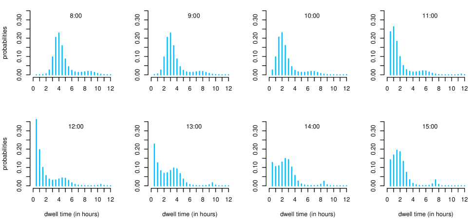
Figure 6: Estimated time-varying dwell-time distributions when initiating high-activity bouts between 8 am and 3 pm under LD condition

As an alternative way of looking into the dwell times implied by the model — not reducing the distributional information but instead averaging over time — the overall dwell-time distributions as derived in Proposition 2.3 are shown in Figure 7. These unconditional dwell-time distributions in the active state emphasize overall differences in the state dynamics between the lighting schedules, specifically showing activity patterns that differ in peak lengths (cf. Figure 5). In particular, the morning and evening activity peaks in the LD condition are relatively short and about equally long, which is reflected by dwell times mostly below five hours. In contrast, the DD condition is characterized by relatively short activity bouts in the morning and notably longer bouts in the evening, leading to a bimodal dwell-time distribution, with considerable mass on lengths of 6–7 hours. These ecologically interesting differences cannot be uncovered when considering only the distributional means, which are fairly similar in both conditions (LD: 2.7 hours; DD: 2.3 hours).

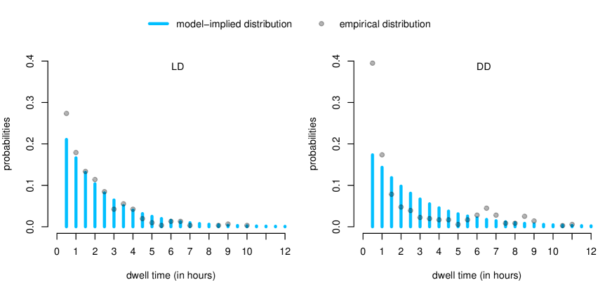
Figure 11: Overall dwell-time distribution of the high-activity state for LD and DD condition, analytically (blue bars) and empirically (gray dots) derived from the fitted homogeneous HMM.

In addition to its inferential use, the unconditional dwell-time distribution constitutes a valuable model-checking tool, as it allows for the comparison of the model-implied dwell times to the empirical ones obtained from the locally decoded state sequence. In the LD condition, we observe a minor lack of fit between the model-implied and the empirical dwell-time distributions, and a very good fit in the DD condition. Compared to the model without temporal variation, which restricts the dwell-time distributions to be geometric, the model fit is substantially improved, especially under the DD condition (see Figure 11 in the Appendix).

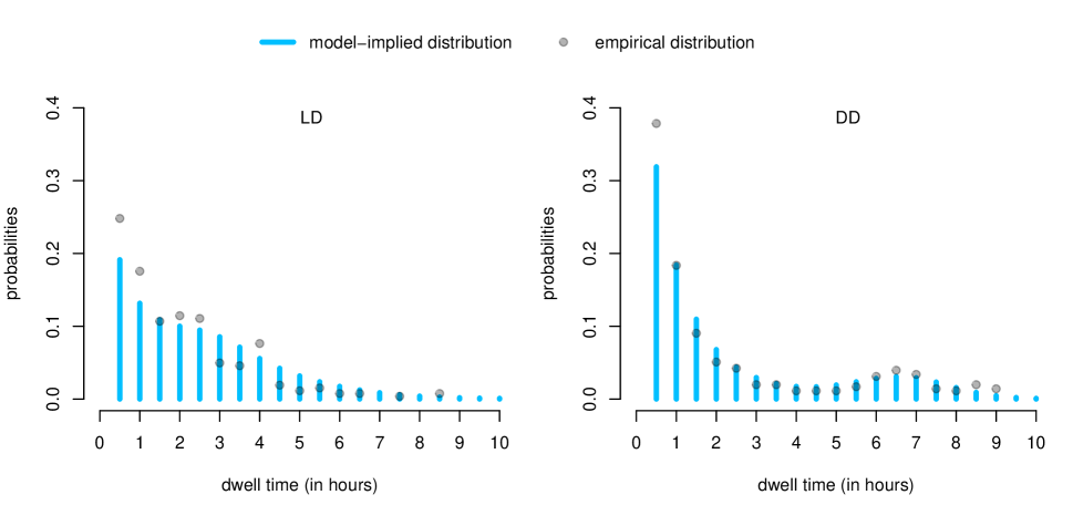
Figure 7: Overall dwell-time distribution of the high-activity state for LD and DD condition, analytically (blue bars) and empirically (gray dots) derived from the fitted HMM.

To summarize, using periodically inhomogeneous HMMs, we showed that fruit flies exhibit a strong diel pattern in activity under a regular light-dark cycle, which does not vanish but becomes more concentrated on the evening hours when subsequently faced with constant darkness. Based on the inferred state dwell-time distributions, the analysis further revealed that dwell times of up to five hours were most likely in the LD condition, whereas dwell times follow a bimodal distribution with mainly very short ($<2$ hours) or long (6–7 hours) durations in the DD condition. These results on common fruit flies’ diel patterns and their adaptations to different lighting schedules will serve as a basis for future research to study variation in genetically mutated flies and their temporal niche mechanisms.

4 Discussion

We established several properties of periodically inhomogeneous Markov chains (and hence also corresponding HMMs), specifically the time-varying (unconditional) state distribution, the time-varying and overall state dwell-time distributions, and a model-checking procedure based on the latter. Knowledge of these properties and tools has welcome implications for applied work using corresponding model formulations.

First, the state distribution as a function of covariates, as displayed for example in Figure 5, is often a key output of interest in empirical analyses based on HMMs. For settings in which the covariate dependence is periodic, for example when modeling diel variation or seasonality, we provide an exact solution to the time-varying state distribution, thus avoiding the need to resort to the approximate solution commonly considered in the literature (Farhadinia et al.,, 2020; Byrnes et al.,, 2021).

Second, our results concerning the state dwell-time distributions provide practitioners with a valuable new inferential tool. In many HMM-based analyses, the stochastic dynamics of the latent state process are of main interest (Jackson et al.,, 2003; McClintock et al.,, 2020). In this regard, our results allow users for the first time to consider and report as an important analysis outcome the true model-implied distribution of time spent in the different states, either at fixed times or as a global summary. This can reveal insights that would otherwise have been missed, for example the second mode of the dwell-time distribution in the flies’ high-activity state when in constant darkness (Figure 7).

As a consequence of our findings related to the state dwell-time distributions, we were able to demonstrate that a common criticism expressed towards basic (homogeneous) HMMs, namely that the implied geometric dwell times are often unrealistic, can to a large extent be remedied by inhomogeneous modeling of the state-switching dynamics. However, substantial deviations from geometric dwell-time distributions will arise only when the data exhibit considerable periodic variation. If a process to be analyzed involves non-geometric dwell-time distributions that can not be explained via periodic variation (or in fact any covariates), then the more flexible class of hidden semi-Markov models, in which an additional distribution on the positive integers is specified to model the dwell times (Guédon,, 2003; Yu,, 2010), is the natural alternative. We suggest the latter approach, in which the unexplained variation in the dwell times is translated into additional model complexity, to be explored only if modeling via inhomogeneous HMMs is not an option or simply insufficient.

Finally, our results allow us to devise a new approach to checking the goodness-of-fit of HMMs involving periodic variation. Established tools for checking the fit of HMMs have focused primarily on the adequacy of the state-dependent process, assessed for example using pseudo-residuals (Buckby et al.,, 2020). In contrast, an inspection of the state dwell-time distributions corresponds to a check whether the system’s state process is being adequately modeled. We thus fill a gaping hole in the HMM toolbox, as the latter should in fact be the central focus of a goodness-of-fit check if the state dynamics are indeed of key interest.

Appendix A Appendix

A.1 Recursive calculation of the periodically stationary distribution

Given a time-varying state distribution $\bm{\delta}^{(t)}$, for any $t\in\{1,\ldots,L\}$, as defined in Equation (3), the remaining $L-1$ stationary distributions can be calculated recursively. More formally, let $\bm{\delta}^{(t)}$ be the solution to $\bm{\delta}^{(t)}\tilde{\bm{\Gamma}}_{t}=\bm{\delta}^{(t)}$. Then

$$\bm{\delta}^{(t+1)}=\bm{\delta}^{(t)}\bm{\Gamma}^{(t)}$$ (6)

is the solution to

$$\bm{\delta}^{(t+1)}\tilde{\bm{\Gamma}}_{t+1}=\bm{\delta}^{(t+1)},$$

since

$$\bm{\delta}^{(t+1)}\tilde{\bm{\Gamma}}_{t+1} =\bm{\delta}^{(t+1)}\bm{\Gamma}^{(t+1)}\bm{\Gamma}^{(t+2)}\dotsc\bm{\Gamma}^{(t+L)}$$

$$=\bm{\delta}^{(t)}\bm{\Gamma}^{(t)}\bm{\Gamma}^{(t+1)}\bm{\Gamma}^{(t+2)}\dotsc\bm{\Gamma}^{(t+L-1)}\bm{\Gamma}^{(t+L)}$$

$$=\bm{\delta}^{(t)}\tilde{\bm{\Gamma}}_{t}\bm{\Gamma}^{(t+L)}=\bm{\delta}^{(t)}\bm{\Gamma}^{(t+L)}$$

$$=\bm{\delta}^{(t)}\bm{\Gamma}^{(t)}=\bm{\delta}^{(t+1)}.$$

A.2 Proofs

Proof of Proposition 2.1.

$$\Pr(S_{t+r}\neq i,S_{t+r-1}=i,\dotsc,S_{t+1}=i\mid S_{t}=i,S_{t-1}\neq i)$$

$$=\Pr(S_{t+r}\neq i,S_{t+r-1}=i,\dotsc,S_{t+1}=i\mid S_{t}=i)$$

$$=\Pr(S_{t+r}\neq i\mid S_{t+r-1}=i)\Pr(S_{t+r-1}=i\mid S_{t+r-2}=i)\dotsc\Pr(S_{t+1}=i\mid S_{t}=i)$$

$$=(1-\gamma_{ii}^{(t+r-1)})\prod_{j=1}^{r-1}\gamma_{ii}^{(t+j-1)}$$

∎

It is evident that the time-varying distribution is identical when the chain has just transitioned into state $i$ or when only conditioning on the chain currently being in state $i$.

Lemma A.1.

Let $\bm{\Gamma}^{(t)}$ be the periodically varying t.p.m of a Markov chain $\{S_{t}\}$ as defined in Equation (1). Then

$$\sum_{r=1}^{L}d_{i}^{(t)}(r)=\sum_{r=1}^{L}\left(1-\gamma_{ii}^{(t+r-1)}\right)\prod_{j=1}^{r-1}\gamma_{ii}^{(j)}=1-\prod_{j=1}^{L}\gamma_{ii}^{(j)}$$

for all $L\in\mathbb{N}$.

Proof.

Without loss of generality, we set $t=1$. We prove the above via induction. For $L=1$, it holds that

$$1-\gamma_{ii}^{(1)}=1-\gamma_{ii}^{(1)}$$

due to the empty product on the left side. If the equality holds for $L$, then it also holds for $L+1$ for every $L\in\mathbb{N}$ since

$$\sum_{r=1}^{L+1}\big{(}1-\gamma_{ii}^{(r)}\big{)}\prod_{j=1}^{r-1}\gamma_{ii}^{(j)}$$

$$=\big{(}1-\gamma_{ii}^{(L+1)}\big{)}\prod_{j=1}^{(L+1)-1}\gamma_{ii}^{(j)}+\sum_{r=1}^{L}\big{(}1-\gamma_{ii}^{(r)}\big{)}\prod_{j=1}^{k-1}\gamma_{ii}^{(j)}$$

$$=\big{(}1-\gamma_{ii}^{(L+1)}\big{)}\prod_{j=1}^{L}\gamma_{ii}^{(j)}+\big{(}1-\prod_{j=1}^{L}\gamma_{ii}^{(j)}\big{)}$$

$$=1-\prod_{j=1}^{L}\gamma_{ii}^{(j)}\big{(}-1+\gamma_{ii}^{(L+1)}+1\big{)}$$

$$=1-\prod_{j=1}^{L}\gamma_{ii}^{(j)}\gamma_{ii}^{(L+1)}$$

$$=1-\prod_{j=1}^{L+1}\gamma_{ii}^{(j)}.$$

We use the induction condition in the second step, the remaining calculations are straightforward. ∎

Proof of Proposition 2.1.

$$\sum_{r=1}^{\infty}rd_{i}^{(t)}(r) =\sum_{r=1}^{\infty}r\bigl{(}1-\gamma_{ii}^{(t+r-1)}\bigr{)}\prod_{j=1}^{r-1}\gamma_{ii}^{(t+j-1)}$$

We can split up the infinite sum into partial sums for each period of length $L$, which gives

$$\sum_{k=0}^{\infty}\sum_{r=kL+1}^{kL+L}r\bigl{(}1-\gamma_{ii}^{(t+r-1)}\bigr{)}\prod_{j=1}^{r-1}\gamma_{ii}^{(t+j-1)}.$$

Then we see that for each $k>0$, i.e. $r>L$, because of Equation (1), at least one full-length product $\prod_{j=1}^{L}\gamma_{ii}^{(j)}$ is contained in each summand. More specifically, a summand with $kL<r\leq(k+1)L$ contains $k$ full-length products, i.e. $(\prod_{j=1}^{L}\gamma_{ii}^{(j)})^{k}$ which is independent of $r$. Therefore we obtain

$$\sum_{k=0}^{\infty}\Bigl{(}\prod_{j=1}^{L}\gamma_{ii}^{(t+j-1)}\Bigr{)}^{k}\sum_{r=kL+1}^{kL+L}r\bigl{(}1-\gamma_{ii}^{(t+r-1)}\bigr{)}\prod_{j=kL+1}^{r-1}\gamma_{ii}^{(t+j-1)}.$$

Now, we see that again by virtue of Equation (1) the remaining product does not depend on the number of periods the chain stays in state $i$. Thus, by changing the indices, we arrive at

$$\sum_{k=0}^{\infty}\Bigl{(}\prod_{j=1}^{L}\gamma_{ii}^{(t+j-1)}\Bigr{)}^{k}\sum_{r=1}^{L}(kL+r)\bigl{(}1-\gamma_{ii}^{(t+r-1)}\bigr{)}\prod_{j=1}^{r-1}\gamma_{ii}^{(t+j-1)}.$$

Multiplying out, we obtain

$$\sum_{k=0}^{\infty}\Bigl{(}\prod_{j=1}^{L}\gamma_{ii}^{(t+j-1)}\Bigr{)}^{k}\Bigl{(}kL\sum_{r=1}^{L}\bigl{(}1-\gamma_{ii}^{(t+r-1)}\bigr{)}\prod_{j=1}^{r-1}\gamma_{ii}^{(t+j-1)}+\sum_{r=1}^{L}r\bigl{(}1-\gamma_{ii}^{(t+r-1)}\bigr{)}\prod_{j=1}^{r-1}\gamma_{ii}^{(t+j-1)}\Bigr{)}$$

$$=\Bigl{(}\sum_{r=1}^{L}r\bigl{(}1-\gamma_{ii}^{(t+r-1)}\bigr{)}\prod_{j=1}^{r-1}\gamma_{ii}^{(t+j-1)}\Bigr{)}\sum_{k=0}^{\infty}\Bigl{(}\prod_{j=1}^{L}\gamma_{ii}^{(t+j-1)}\Bigr{)}^{k}$$

$$+L\Bigl{(}\sum_{r=1}^{L}\bigl{(}1-\gamma_{ii}^{(t+r-1)}\bigr{)}\prod_{j=1}^{r-1}\gamma_{ii}^{(t+j-1)}\Bigr{)}\sum_{k=0}^{\infty}k\Bigl{(}\prod_{j=1}^{L}\gamma_{ii}^{(t+j-1)}\Bigr{)}^{k}.$$

Assuming $\gamma_{ii}^{(t)}<1\text{ for all }t$ we can use the geometric sum and its derivative to calculate the infinite sums, which gives

$$\frac{\sum_{r=1}^{L}r\bigl{(}1-\gamma_{ii}^{(t+r-1)}\bigr{)}\prod_{j=1}^{r-1}\gamma_{ii}^{(t+j-1)}}{1-\prod_{j=1}^{L}\gamma_{ii}^{(t+j-1)}}+L\Bigl{(}\sum_{r=1}^{L}\bigl{(}1-\gamma_{ii}^{(t+r-1)}\bigr{)}\prod_{j=1}^{r-1}\gamma_{ii}^{(t+j-1)}\Bigr{)}\frac{\prod_{j=1}^{L}\gamma_{ii}^{(t+j-1)}}{\bigl{(}1-\prod_{j=1}^{L}\gamma_{ii}^{(t+j-1)}\bigr{)}^{2}}.$$

Now we employ Lemma A.1 in the second summand to obtain

$$\frac{\sum_{r=1}^{L}r\bigl{(}1-\gamma_{ii}^{(t+r-1)}\bigr{)}\prod_{j=1}^{r-1}\gamma_{ii}^{(t+j-1)}}{1-\prod_{j=1}^{L}\gamma_{ii}^{(t+j-1)}}+L\Bigl{(}1-\prod_{j=1}^{L}\gamma_{ii}^{(t+j-1)}\Bigr{)}\frac{\prod_{j=1}^{L}\gamma_{ii}^{(t+j-1)}}{\bigl{(}1-\prod_{j=1}^{L}\gamma_{ii}^{(t+j-1)}\bigr{)}^{2}}$$

$$=\frac{\sum_{r=1}^{L}rd_{i}^{(t)}(r)+L\prod_{j=1}^{L}\gamma_{ii}^{(t+j-1)}}{1-\prod_{j=1}^{L}\gamma_{ii}^{(t+j-1)}}.$$

We employ Lemma A.1 a second time in the numerator and denominator yielding

$$\frac{\sum_{r=1}^{L}rd_{i}^{(t)}(r)+L\bigl{(}1-\sum_{r=1}^{L}d_{i}^{(t)}(r)\bigr{)}}{\sum_{r=1}^{L}d_{i}^{(t)}(r)}$$

$$=\frac{\sum_{r=1}^{L}rd_{i}^{(t)}(r)+L-L\sum_{r=1}^{L}d_{i}^{(t)}(r)}{\sum_{r=1}^{L}d_{i}^{(t)}(r)}$$

$$=\frac{L+\sum_{r=1}^{L}rd_{i}^{(t)}(r)}{\sum_{r=1}^{L}d_{i}^{(t)}(r)}-L.$$

∎

Proof of Proposition 2.3.

We need to obtain the overall dwell-time distribution as a mixture of the time-varying dwell-time distributions. For the weighting, we need to consider a random variable $\tau$ on the support $\{1,\dotsc,L\}$ that is uniformly distributed with $\Pr(\tau=t)=\frac{1}{L}$ for all $t=1,\dotsc,L$. The realization of $\tau$ gives rise to every time point $t\in\{1,\dotsc,L\}$ considered in the mixture as a starting time for a dwell time. Then we can rewrite the time-varying dwell-time distributions as

$$d_{i}^{(t)}(r)=\Pr(S_{\tau+r}\neq i,S_{\tau+r-1}=i,\dotsc,S_{\tau+1}=i\mid S_{\tau}=i,S_{\tau-1}\neq i,\tau=t).$$

The probability we are interested in as the overall dwell-time distribution is

$$\Pr(S_{\mathchoice{\mathbin{\vbox{\hbox{\scalebox{0.5}{$\displaystyle\bullet$}}}}}{\mathbin{\vbox{\hbox{\scalebox{0.5}{$\textstyle\bullet$}}}}}{\mathbin{\vbox{\hbox{\scalebox{0.5}{$\scriptstyle\bullet$}}}}}{\mathbin{\vbox{\hbox{\scalebox{0.5}{$\scriptscriptstyle\bullet$}}}}}+r}\neq i,S_{\mathchoice{\mathbin{\vbox{\hbox{\scalebox{0.5}{$\displaystyle\bullet$}}}}}{\mathbin{\vbox{\hbox{\scalebox{0.5}{$\textstyle\bullet$}}}}}{\mathbin{\vbox{\hbox{\scalebox{0.5}{$\scriptstyle\bullet$}}}}}{\mathbin{\vbox{\hbox{\scalebox{0.5}{$\scriptscriptstyle\bullet$}}}}}+r-1}=i,\dots,S_{\mathchoice{\mathbin{\vbox{\hbox{\scalebox{0.5}{$\displaystyle\bullet$}}}}}{\mathbin{\vbox{\hbox{\scalebox{0.5}{$\textstyle\bullet$}}}}}{\mathbin{\vbox{\hbox{\scalebox{0.5}{$\scriptstyle\bullet$}}}}}{\mathbin{\vbox{\hbox{\scalebox{0.5}{$\scriptscriptstyle\bullet$}}}}}+1}=i\mid S_{\mathchoice{\mathbin{\vbox{\hbox{\scalebox{0.5}{$\displaystyle\bullet$}}}}}{\mathbin{\vbox{\hbox{\scalebox{0.5}{$\textstyle\bullet$}}}}}{\mathbin{\vbox{\hbox{\scalebox{0.5}{$\scriptstyle\bullet$}}}}}{\mathbin{\vbox{\hbox{\scalebox{0.5}{$\scriptscriptstyle\bullet$}}}}}}=i,S_{\mathchoice{\mathbin{\vbox{\hbox{\scalebox{0.5}{$\displaystyle\bullet$}}}}}{\mathbin{\vbox{\hbox{\scalebox{0.5}{$\textstyle\bullet$}}}}}{\mathbin{\vbox{\hbox{\scalebox{0.5}{$\scriptstyle\bullet$}}}}}{\mathbin{\vbox{\hbox{\scalebox{0.5}{$\scriptscriptstyle\bullet$}}}}}-1}\neq i).$$

The dot notation is used to emphasize that this probability for the Markov chain to transition to state $i$ from any other state and to then stay in state $i$ $r$ times is unconditional of the time point in the cycle. We condition on the event that the transition $\neg i\rightarrow i$ has happened at some arbitrary time point in the cycle, prior to the stay. Then, we can obtain the overall dwell-time distribution as

$$d_{i}(r) =\Pr(S_{\mathchoice{\mathbin{\vbox{\hbox{\scalebox{0.5}{$\displaystyle\bullet$}}}}}{\mathbin{\vbox{\hbox{\scalebox{0.5}{$\textstyle\bullet$}}}}}{\mathbin{\vbox{\hbox{\scalebox{0.5}{$\scriptstyle\bullet$}}}}}{\mathbin{\vbox{\hbox{\scalebox{0.5}{$\scriptscriptstyle\bullet$}}}}}+r}\neq i,S_{\mathchoice{\mathbin{\vbox{\hbox{\scalebox{0.5}{$\displaystyle\bullet$}}}}}{\mathbin{\vbox{\hbox{\scalebox{0.5}{$\textstyle\bullet$}}}}}{\mathbin{\vbox{\hbox{\scalebox{0.5}{$\scriptstyle\bullet$}}}}}{\mathbin{\vbox{\hbox{\scalebox{0.5}{$\scriptscriptstyle\bullet$}}}}}+r-1}=i,\dotsc,S_{\mathchoice{\mathbin{\vbox{\hbox{\scalebox{0.5}{$\displaystyle\bullet$}}}}}{\mathbin{\vbox{\hbox{\scalebox{0.5}{$\textstyle\bullet$}}}}}{\mathbin{\vbox{\hbox{\scalebox{0.5}{$\scriptstyle\bullet$}}}}}{\mathbin{\vbox{\hbox{\scalebox{0.5}{$\scriptscriptstyle\bullet$}}}}}+1}=i\mid S_{\mathchoice{\mathbin{\vbox{\hbox{\scalebox{0.5}{$\displaystyle\bullet$}}}}}{\mathbin{\vbox{\hbox{\scalebox{0.5}{$\textstyle\bullet$}}}}}{\mathbin{\vbox{\hbox{\scalebox{0.5}{$\scriptstyle\bullet$}}}}}{\mathbin{\vbox{\hbox{\scalebox{0.5}{$\scriptscriptstyle\bullet$}}}}}}=i,S_{\mathchoice{\mathbin{\vbox{\hbox{\scalebox{0.5}{$\displaystyle\bullet$}}}}}{\mathbin{\vbox{\hbox{\scalebox{0.5}{$\textstyle\bullet$}}}}}{\mathbin{\vbox{\hbox{\scalebox{0.5}{$\scriptstyle\bullet$}}}}}{\mathbin{\vbox{\hbox{\scalebox{0.5}{$\scriptscriptstyle\bullet$}}}}}-1}\neq i)$$

$$=\frac{\Pr(S_{\mathchoice{\mathbin{\vbox{\hbox{\scalebox{0.5}{$\displaystyle\bullet$}}}}}{\mathbin{\vbox{\hbox{\scalebox{0.5}{$\textstyle\bullet$}}}}}{\mathbin{\vbox{\hbox{\scalebox{0.5}{$\scriptstyle\bullet$}}}}}{\mathbin{\vbox{\hbox{\scalebox{0.5}{$\scriptscriptstyle\bullet$}}}}}+r}\neq i,S_{\mathchoice{\mathbin{\vbox{\hbox{\scalebox{0.5}{$\displaystyle\bullet$}}}}}{\mathbin{\vbox{\hbox{\scalebox{0.5}{$\textstyle\bullet$}}}}}{\mathbin{\vbox{\hbox{\scalebox{0.5}{$\scriptstyle\bullet$}}}}}{\mathbin{\vbox{\hbox{\scalebox{0.5}{$\scriptscriptstyle\bullet$}}}}}+r-1}=i,\dotsc,S_{\mathchoice{\mathbin{\vbox{\hbox{\scalebox{0.5}{$\displaystyle\bullet$}}}}}{\mathbin{\vbox{\hbox{\scalebox{0.5}{$\textstyle\bullet$}}}}}{\mathbin{\vbox{\hbox{\scalebox{0.5}{$\scriptstyle\bullet$}}}}}{\mathbin{\vbox{\hbox{\scalebox{0.5}{$\scriptscriptstyle\bullet$}}}}}+1}=i,S_{\mathchoice{\mathbin{\vbox{\hbox{\scalebox{0.5}{$\displaystyle\bullet$}}}}}{\mathbin{\vbox{\hbox{\scalebox{0.5}{$\textstyle\bullet$}}}}}{\mathbin{\vbox{\hbox{\scalebox{0.5}{$\scriptstyle\bullet$}}}}}{\mathbin{\vbox{\hbox{\scalebox{0.5}{$\scriptscriptstyle\bullet$}}}}}}=i,S_{\mathchoice{\mathbin{\vbox{\hbox{\scalebox{0.5}{$\displaystyle\bullet$}}}}}{\mathbin{\vbox{\hbox{\scalebox{0.5}{$\textstyle\bullet$}}}}}{\mathbin{\vbox{\hbox{\scalebox{0.5}{$\scriptstyle\bullet$}}}}}{\mathbin{\vbox{\hbox{\scalebox{0.5}{$\scriptscriptstyle\bullet$}}}}}-1}\neq i)}{\Pr(S_{\mathchoice{\mathbin{\vbox{\hbox{\scalebox{0.5}{$\displaystyle\bullet$}}}}}{\mathbin{\vbox{\hbox{\scalebox{0.5}{$\textstyle\bullet$}}}}}{\mathbin{\vbox{\hbox{\scalebox{0.5}{$\scriptstyle\bullet$}}}}}{\mathbin{\vbox{\hbox{\scalebox{0.5}{$\scriptscriptstyle\bullet$}}}}}}=i,S_{\mathchoice{\mathbin{\vbox{\hbox{\scalebox{0.5}{$\displaystyle\bullet$}}}}}{\mathbin{\vbox{\hbox{\scalebox{0.5}{$\textstyle\bullet$}}}}}{\mathbin{\vbox{\hbox{\scalebox{0.5}{$\scriptstyle\bullet$}}}}}{\mathbin{\vbox{\hbox{\scalebox{0.5}{$\scriptscriptstyle\bullet$}}}}}-1}\neq i)}$$

$$=\frac{\sum_{t=1}^{L}\Pr(S_{\tau+r}\neq i,S_{\tau+r-1}=i,\dotsc,S_{\tau+1}=i,S_{\tau}=i,S_{\tau-1}\neq i,\tau=t)}{\Pr(S_{\mathchoice{\mathbin{\vbox{\hbox{\scalebox{0.5}{$\displaystyle\bullet$}}}}}{\mathbin{\vbox{\hbox{\scalebox{0.5}{$\textstyle\bullet$}}}}}{\mathbin{\vbox{\hbox{\scalebox{0.5}{$\scriptstyle\bullet$}}}}}{\mathbin{\vbox{\hbox{\scalebox{0.5}{$\scriptscriptstyle\bullet$}}}}}}=i,S_{\mathchoice{\mathbin{\vbox{\hbox{\scalebox{0.5}{$\displaystyle\bullet$}}}}}{\mathbin{\vbox{\hbox{\scalebox{0.5}{$\textstyle\bullet$}}}}}{\mathbin{\vbox{\hbox{\scalebox{0.5}{$\scriptstyle\bullet$}}}}}{\mathbin{\vbox{\hbox{\scalebox{0.5}{$\scriptscriptstyle\bullet$}}}}}-1}\neq i)}$$

$$=\sum_{t=1}^{L}\Pr(S_{\tau+r}\neq i,S_{\tau+r-1}=i,\dotsc,S_{\tau+1}=i\mid S_{\tau}=i,S_{\tau-1}\neq i,\tau=t)$$

$$\qquad\frac{\Pr(S_{\tau}=i,S_{\tau-1}\neq i,\tau=t)}{\Pr(S_{\mathchoice{\mathbin{\vbox{\hbox{\scalebox{0.5}{$\displaystyle\bullet$}}}}}{\mathbin{\vbox{\hbox{\scalebox{0.5}{$\textstyle\bullet$}}}}}{\mathbin{\vbox{\hbox{\scalebox{0.5}{$\scriptstyle\bullet$}}}}}{\mathbin{\vbox{\hbox{\scalebox{0.5}{$\scriptscriptstyle\bullet$}}}}}}=i,S_{\mathchoice{\mathbin{\vbox{\hbox{\scalebox{0.5}{$\displaystyle\bullet$}}}}}{\mathbin{\vbox{\hbox{\scalebox{0.5}{$\textstyle\bullet$}}}}}{\mathbin{\vbox{\hbox{\scalebox{0.5}{$\scriptstyle\bullet$}}}}}{\mathbin{\vbox{\hbox{\scalebox{0.5}{$\scriptscriptstyle\bullet$}}}}}-1}\neq i)}$$

$$=\sum_{t=1}^{L}d_{i}^{(t)}(r)w_{i}^{(t)}.$$

We now need to show that we can calculate the mixture weights explicitly to arrive at the mixture weights $w_{i}^{(t)}$ as defined before, precisely that

$$w_{i}^{(t)} =\frac{\Pr(S_{\tau}=i,S_{\tau-1}\neq i,\tau=t)}{\Pr(S_{\mathchoice{\mathbin{\vbox{\hbox{\scalebox{0.5}{$\displaystyle\bullet$}}}}}{\mathbin{\vbox{\hbox{\scalebox{0.5}{$\textstyle\bullet$}}}}}{\mathbin{\vbox{\hbox{\scalebox{0.5}{$\scriptstyle\bullet$}}}}}{\mathbin{\vbox{\hbox{\scalebox{0.5}{$\scriptscriptstyle\bullet$}}}}}}=i,S_{\mathchoice{\mathbin{\vbox{\hbox{\scalebox{0.5}{$\displaystyle\bullet$}}}}}{\mathbin{\vbox{\hbox{\scalebox{0.5}{$\textstyle\bullet$}}}}}{\mathbin{\vbox{\hbox{\scalebox{0.5}{$\scriptstyle\bullet$}}}}}{\mathbin{\vbox{\hbox{\scalebox{0.5}{$\scriptscriptstyle\bullet$}}}}}-1}\neq i)}$$

$$=\frac{\sum_{l\in\mathcal{S}\setminus i}\delta_{l}^{(t-1)}\gamma_{li}^{(t-1)}}{\sum_{t=1}^{L}\sum_{l\in\mathcal{S}\setminus i}\delta_{l}^{(t-1)}\gamma_{li}^{(t-1)}},$$

where $\mathcal{S}=\{1,\dotsc,N\}$. We therefore consider the numerator and denominator separately. For the numerator, we need to consider all possible paths of the Markov chain from all states $l\neq i$ to state $i$:

$$\Pr(S_{\tau}=i,S_{\tau-1}\neq i,\tau=t) =\sum_{l\in\mathcal{S}\setminus i}\Pr(S_{\tau}=i\mid S_{\tau-1}=l,\tau=t)\Pr(S_{\tau-1}=l\mid\tau=t)\Pr(\tau=t)$$

$$=\sum_{l\in\mathcal{S}\setminus i}\delta_{l}^{(t-1)}\gamma_{li}^{(t-1)}\frac{1}{L}.$$

For the denominator, we obtain

$$\Pr(S_{\mathchoice{\mathbin{\vbox{\hbox{\scalebox{0.5}{$\displaystyle\bullet$}}}}}{\mathbin{\vbox{\hbox{\scalebox{0.5}{$\textstyle\bullet$}}}}}{\mathbin{\vbox{\hbox{\scalebox{0.5}{$\scriptstyle\bullet$}}}}}{\mathbin{\vbox{\hbox{\scalebox{0.5}{$\scriptscriptstyle\bullet$}}}}}}=i,S_{\mathchoice{\mathbin{\vbox{\hbox{\scalebox{0.5}{$\displaystyle\bullet$}}}}}{\mathbin{\vbox{\hbox{\scalebox{0.5}{$\textstyle\bullet$}}}}}{\mathbin{\vbox{\hbox{\scalebox{0.5}{$\scriptstyle\bullet$}}}}}{\mathbin{\vbox{\hbox{\scalebox{0.5}{$\scriptscriptstyle\bullet$}}}}}-1}\neq i) =\sum_{t=1}^{L}\Pr(S_{\tau}=i,S_{\tau-1}\neq i,\tau=t)$$

$$=\frac{1}{L}\sum_{t=1}^{L}\sum_{l\in\mathcal{S}\setminus i}\delta_{l}^{(t-1)}\gamma_{li}^{(t-1)}.$$

Furthermore, we can calculate the mean of the distribution as

$$\mathbb{E}R_{i} =\sum_{r=1}^{\infty}rd_{i}(r)$$

$$=\sum_{r=1}^{\infty}r\sum_{t=1}^{L}w_{i}^{(t)}d_{i}^{(t)}(r)$$

$$=\sum_{t=1}^{L}w_{i}^{(t)}\sum_{r=1}^{\infty}rd_{i}^{(t)}(r)$$

$$=\sum_{t=1}^{L}w_{i}^{(t)}\mathbb{E}R_{i}^{(t)}$$

$$=\sum_{t=1}^{L}w_{i}^{(t)}\left(\frac{L+\sum_{r=1}^{L}rd_{i}^{(t)}(r)}{\sum_{r=1}^{L}d_{i}^{(t)}(r)}-L\right)$$

$$=\sum_{t=1}^{L}w_{i}^{(t)}\frac{L+\sum_{r=1}^{L}rd_{i}^{(t)}(r)}{\sum_{r=1}^{L}d_{i}^{(t)}(r)}-L\sum_{t=1}^{L}w_{i}^{(t)}$$

$$=\sum_{t=1}^{L}\left(w_{i}^{(t)}\frac{L+\sum_{r=1}^{L}rd_{i}^{(t)}(r)}{\sum_{r=1}^{L}d_{i}^{(t)}(r)}\right)-L,$$

where the third equality is justified by the Fubini-Tonelli-theorem. ∎

A.3 Additional figures

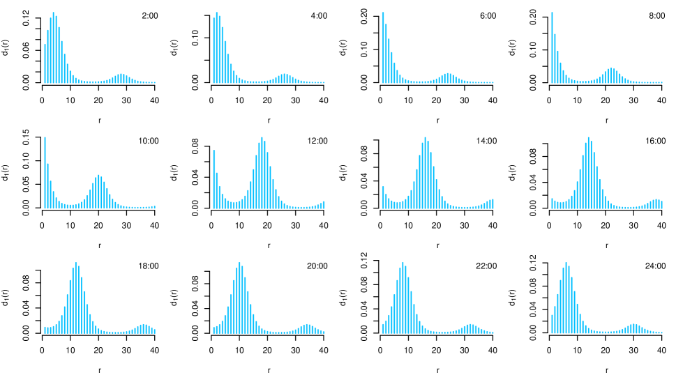
Figure 8: Time-varying dwell-time distribution (state 2) of an example 2-state HMM with trigonometric modeling of periodic variation (see Appendix A.4 for the precise model configuration).

A.4 Parameters used for Figures 3, 4 and 8

Figures 3, 4 and 8 were generated based on 2-state HMMs with the entries of the t.p.m. modeled as specified in Equation (2). The parameter values used for Figure 3 are

$$\bm{\beta}^{(12)}=(-1.2,0.85,0.15)\quad\text{and}\quad\bm{\beta}^{(21)}=(-1.5,-0.7,-1.3),$$

those for Figures 4 and 8 are

$$\bm{\beta}^{(12)}=(-3,1.5,-0.9)\quad\text{and}\quad\bm{\beta}^{(21)}=(-3,1.2,-1.1).$$

References

- Beaver et al., (2002) Beaver, L., Gvakharia, B., Vollintine, T., Hege, D., Stanewsky, R., and Giebultowicz, J. (2002). Loss of circadian clock function decreases reproductive fitness in males of drosophila melanogaster. Proceedings of the National Academy of Sciences, 99(4):2134–2139.
- Bernhardt et al., (2020) Bernhardt, J. R., O’Connor, M. I., Sunday, J. M., and Gonzalez, A. (2020). Life in fluctuating environments. Philosophical Transactions of the Royal Society B, 375(1814):20190454.
- Beumer et al., (2020) Beumer, L. T., Pohle, J., Schmidt, N. M., Chimienti, M., Desforges, J.-P., Hansen, L. H., Langrock, R., Pedersen, S. H., Stelvig, M., and van Beest, F. M. (2020). An application of upscaled optimal foraging theory using hidden Markov modelling: year-round behavioural variation in a large arctic herbivore. Movement Ecology, 8:1–16.
- Buckby et al., (2020) Buckby, J., Wang, T., Zhuang, J., and Obara, K. (2020). Model checking for hidden Markov models. Journal of Computational and Graphical Statistics, 29(4):859–874.
- Byrnes et al., (2021) Byrnes, E. E., Daly, R., Leos-Barajas, V., Langrock, R., and Gleiss, A. C. (2021). Evaluating the constraints governing activity patterns of a coastal marine top predator. Marine Biology, 168(1):11.
- Farhadinia et al., (2020) Farhadinia, M. S., Michelot, T., Johnson, P. J., Hunter, L. T., and Macdonald, D. W. (2020). Understanding decision making in a food-caching predator using hidden Markov models. Movement Ecology, 8:1–13.
- Feldmann et al., (2023) Feldmann, C. C., Mews, S., Coculla, A., Stanewsky, R., and Langrock, R. (2023). Flexible modelling of diel and other periodic variation in hidden Markov models. Journal of Statistical Theory and Practice, 17(45):1–15.
- Ge et al., (2006) Ge, H., Jiang, D.-Q., and Qian, M. (2006). A simple discrete model of brownian motors: Time-periodic Markov chains. Journal of Statistical Physics, 123(4):831–859.
- Gerber and Furrer, (2019) Gerber, F. and Furrer, R. (2019). optimparallel: An R package providing a parallel version of the L-BFGS-B optimization method. The R Journal, 11(1):352–358.
- Guédon, (2003) Guédon, Y. (2003). Estimating hidden semi-Markov chains from discrete sequences. Journal of Computational and Graphical Statistics, 12(3):604–639.
- Hertel et al., (2017) Hertel, A. G., Swenson, J. E., and Bischof, R. (2017). A case for considering individual variation in diel activity patterns. Behavioral Ecology, 28(6):1524–1531.
- Hussey et al., (2015) Hussey, N. E., Kessel, S. T., Aarestrup, K., Cooke, S. J., Cowley, P. D., Fisk, A. T., Harcourt, R. G., Holland, K. N., Iverson, S. J., Kocik, J. F., et al. (2015). Aquatic animal telemetry: a panoramic window into the underwater world. Science, 348(6240):1255642.
- Jackson et al., (2003) Jackson, C. H., Sharples, L. D., Thompson, S. G., Duffy, S. W., and Couto, E. (2003). Multistate Markov models for disease progression with classification error. Journal of the Royal Statistical Society Series D: The Statistician, 52(2):193–209.
- Jannetti et al., (2019) Jannetti, M. G., Buck, C. L., Valentinuzzi, V. S., and Oda, G. A. (2019). Day and night in the subterranean: measuring daily activity patterns of subterranean rodents (ctenomys aff. knighti) using bio-logging. Conservation Physiology, 7(1):coz044.
- Kargapolova and Ogorodnikov, (2012) Kargapolova, N. A. and Ogorodnikov, V. A. (2012). Inhomogeneous Markov chains with periodic matrices of transition probabilities and their application to simulation of meteorological processes. Russian Journal of Numerical Analysis and Mathematical Modelling, 27(3):213–228.
- Kays et al., (2015) Kays, R., Crofoot, M. C., Jetz, W., and Wikelski, M. (2015). Terrestrial animal tracking as an eye on life and planet. Science, 348(6240):aaa2478.
- Langrock et al., (2012) Langrock, R., King, R., Matthiopoulos, J., Thomas, L., Fortin, D., and Morales, J. M. (2012). Flexible and practical modeling of animal telemetry data: hidden Markov models and extensions. Ecology, 93(11):2336–2342.
- Leos-Barajas et al., (2017) Leos-Barajas, V., Photopoulou, T., Langrock, R., Patterson, T. A., Watanabe, Y. Y., Murgatroyd, M., and Papastamatiou, Y. P. (2017). Analysis of animal accelerometer data using hidden Markov models. Methods in Ecology and Evolution, 8(2):161–173.
- Li and Bolker, (2017) Li, M. and Bolker, B. M. (2017). Incorporating periodic variability in hidden Markov models for animal movement. Movement Ecology, 5(1):1–12.
- McClintock et al., (2020) McClintock, B. T., Langrock, R., Gimenez, O., Cam, E., Borchers, D. L., Glennie, R., and Patterson, T. A. (2020). Uncovering ecological state dynamics with hidden Markov models. Ecology Letters, 23(12):1878–1903.
- Nathan et al., (2022) Nathan, R., Monk, C. T., Arlinghaus, R., Adam, T., Alós, J., Assaf, M., Baktoft, H., Beardsworth, C. E., Bertram, M. G., Bijleveld, A. I., et al. (2022). Big-data approaches lead to an increased understanding of the ecology of animal movement. Science, 375(6582):eabg1780.
- Patterson et al., (2009) Patterson, T. A., Basson, M., Bravington, M. V., and Gunn, J. S. (2009). Classifying movement behaviour in relation to environmental conditions using hidden Markov models. Journal of Animal Ecology, 78(6):1113–1123.
- Patterson et al., (2017) Patterson, T. A., Parton, A., Langrock, R., Blackwell, P. G., Thomas, L., and King, R. (2017). Statistical modelling of individual animal movement: an overview of key methods and a discussion of practical challenges. AStA Advances in Statistical Analysis, 101:399–438.
- Pohle et al., (2017) Pohle, J., Langrock, R., Van Beest, F. M., and Schmidt, N. M. (2017). Selecting the number of states in hidden Markov models: pragmatic solutions illustrated using animal movement. Journal of Agricultural, Biological and Environmental Statistics, 22:270–293.
- R Core Team, (2023) R Core Team (2023). R: A Language and Environment for Statistical Computing. R Foundation for Statistical Computing, Vienna, Austria.
- Schliehe-Diecks et al., (2012) Schliehe-Diecks, S., Kappeler, P., and Langrock, R. (2012). On the application of mixed hidden Markov models to multiple behavioural time series. Interface Focus, 2(2):180–189.
- Touron, (2019) Touron, A. (2019). Consistency of the maximum likelihood estimator in seasonal hidden Markov models. Statistics and Computing, 29(5):1055–1075.
- Weegman et al., (2017) Weegman, M. D., Bearhop, S., Hilton, G. M., Walsh, A. J., Griffin, L., Resheff, Y. S., Nathan, R., and David Fox, A. (2017). Using accelerometry to compare costs of extended migration in an arctic herbivore. Current Zoology, 63(6):667–674.
- Yu, (2010) Yu, S.-Z. (2010). Hidden semi-Markov models. Artificial intelligence, 174(2):215–243.