MMGPL: Multimodal Medical Data Analysis with Graph Prompt Learning

Abstract

Prompt learning has demonstrated impressive efficacy in the fine-tuning of multimodal large models to a wide range of downstream tasks. Nonetheless, applying existing prompt learning methods for the diagnosis of neurological disorder still suffers from two issues: (i) existing methods typically treat all patches equally, despite the fact that only a small number of patches in neuroimaging are relevant to the disease, and (ii) they ignore the structural information inherent in the brain connection network which is crucial for understanding and diagnosing neurological disorders. To tackle these issues, we introduce a novel prompt learning model by learning graph prompts during the fine-tuning process of multimodal large models for diagnosing neurological disorders. Specifically, we first leverage GPT-4 to obtain relevant disease concepts and compute semantic similarity between these concepts and all patches. Secondly, we reduce the weight of irrelevant patches according to the semantic similarity between each patch and disease-related concepts. Moreover, we construct a graph among tokens based on these concepts and employ a graph convolutional network layer to extract the structural information of the graph, which is used to prompt the pre-trained multimodal large models for diagnosing neurological disorders. Extensive experiments demonstrate that our method achieves superior performance for neurological disorder diagnosis compared with state-of-the-art methods and validated by clinicians.

I Introduction

Neurological disorders, including Autism Spectrum Disorder (ASD) (Lord et al., 2018) and Alzheimer’s Disease (AD) (Scheltens et al., 2021), severely impair subjects’ social, linguistic, and cognitive abilities, and have already become serious public health issues worldwide (Feigin et al., 2020). Unfortunately, there are no definitive cures for most neurological disorders (e.g., ASD and AD), so diagnosis of neurological disorder is urgently needed to promote early intervention and delay its deterioration (Wingo et al., 2021; Zhu et al., 2022). Over the last decade, researchers (Wen et al., 2020; Li et al., 2021; Dvornek et al., 2019) have applied various machine learning methods, such as Convolutional Neural Networks (CNN) LeCun and Bengio (1995), Graph Neural Networks (GNN) Kipf and Welling (2017), and Recurrent Neural Networks (RNN) Schuster and Paliwal (1997), to diagnose neurological disorders. Despite the remarkable progress made by these methods, the robustness and effectiveness of these deep learning models are difficult to ensure due to the fact that these methods are directly trained on small-scale and complicated medical datasets (Dinsdale et al., 2022).

Recently, multimodal large models (Liu et al., 2023; Driess et al., 2023; Tu et al., 2023; Wu et al., 2023) with extensive parameters, trained on vast datasets and diverse tasks, have exhibited remarkable generality and adaptability. As a result, multimodal large models have become a recent focal point within the field of medical data analysis. Researchers across various domains have developed disparate products such as the large language models (e.g., GPT (OpenAI, 2023)) and the large vision models (e.g., SAM (Kirillov et al., 2023)). They can accelerate the development of accurate and robust models, reducing reliance on extensive labeled data (Zhang and Metaxas, 2023). Owing to their generality, multimodal large models hold immense potential in addressing a wide array of diagnostic tasks for neurological disorders.

However, applying these multimodal large models in the field of neurological disorders diagnosis faces significant challenges due to the diverse modalities in multimodal medical data (e.g., PET and MRI), which differ greatly from natural images. To fill the gap between the pre-training tasks and downstream tasks, researchers utilize techniques such as full fine-tuning and prompt learning on pre-trained multimodal large models to address specific downstream tasks in medicine domains. Specifically, full fine-tuning is a commonly used method in transfer learning, which updates the weights of pre-trained models on task-specific data. However, full fine-tuning methods (Howard and Ruder, 2018) are becoming increasingly difficult to operate when dealing with large models with massive parameters because they require fine-tuning the entire model directly. Recently, prompt learning (Brown et al., 2020) has become a new fine-tuning paradigm of modern multimodal large models, which explicit instructions or adjusts only a small portion of parameters of prompts to guide the foundation model. For example, Lester et al. (2021) demonstrates that even for models of the 10 billion parameter scale, optimizing the prompt alone while keeping the model parameters fixed can achieve performance comparable to that of full fine-tuning.

Despite the impressive results demonstrated by prompt learning, it is highly task-specific, requiring researchers from different domains to design customized prompts to maximize its potential. In the field of Natural Language Processing (NLP), previous works usually employed cloze prompts, which can be designed manually or automatically. For example, Brown et al. (2020) manually defines specific prompt templates to boost various NLP tasks. However, manually adjusting the prompt templates lacks flexibility and efficiency. To yield more flexible and efficient prompts, many researchers (Lu et al., 2022; Gao et al., 2020; Schick and Schütze, 2020) proposed to discover prompts through automatic learning under supervised data. Inspired by the successful application of prompt learning in NLP, researchers have started exploring prompt learning in computer vision (CV). For instance, VPT (Jia et al., 2022) proposed a single-modality prompt learning method that designs individual prompts for images. However, single-modality prompt learning method only prompts one modality and ignores the prompt from the other modality. To yield more effective prompt learning, (Khattak et al., 2023; Zhou et al., 2022) designed to prompt both image modality and text modality. Despite the widespread application of prompt learning methods in the fields of NLP and CV, we still face challenges when applying prompt learning to fill the gap between the pre-training multimodal large models and the diagnosis of neurological disorders.

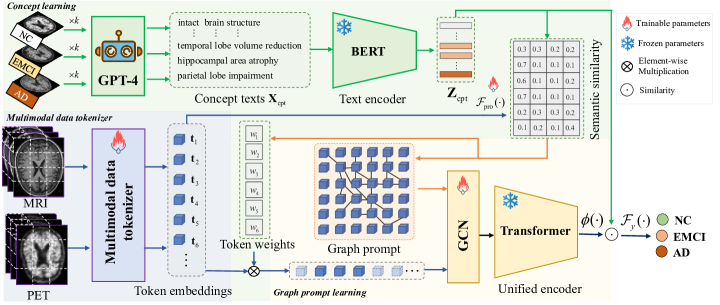
Figure 1: The flowchart of the proposed MMGPL consisting of three modules i.e., multimodal data tokenizer (light blue block), concept learning (light green block), and graph prompt learning (light yellow block). First, we first divide the raw multimodal data into multiple patches and project them into a shared embedding space (Sec. III-B). Second, we prompt the GPT-4 to generate disease-related concepts and further learn the weights of tokens based on the semantic similarity between tokens and concepts (Sec. III-C). Third, We learn a graph among tokens and extract structural information to prompt the unified encoder (Sec. III-D). Finally, we obtain the output from the unified encoder and use it to predict the label of the subject.

Firstly, only a small fraction of patches in neural data are related to the disease. Unlike natural image data, the pathological regions or the regions of interest (i.e., ROIs) in neural data typically only occupy a small portion of the entire data. For example, previous studies (Padurariu et al., 2012; Wang et al., 2006) have shown a significant correlation between the hippocampal area and Alzheimer’s disease. Recently, in the area of medical image segmentation, methods (Huang et al., 2023; Zhang et al., 2023b) utilize region-based prompts, such as bounding boxes and clicks, to guide the fundamental model focus on ROIs within the medical images. Despite the promising results obtained by region-based prompts, the aforementioned operations (e.g., bounding box and clicks) often rely on human interaction or object detection models which reduces the flexibility of these methods. Moreover, implementing the aforementioned operations becomes even more challenging when dealing with multimodality neural data, which may typically contains 3D tensor MRI data, time-series data, and functional connectivity (FC) networks data. Hence, it is challenging to discover useful patches when dealing with multimodality neural data.

Secondly, the structural information among patches plays a crucial role in the analysis of neurological disorders. In the field of neuroscience, researchers (Bullmore and Sporns, 2009; Fornito et al., 2015) have indicated that the brain is a complex and interconnected network/graph, and the connection topology (i.e., structural information) of the brain fundamentally shapes the progression of neurological disorders. Although the transformer architecture includes a graph block (i.e., composed of keys, queries, and values) for extracting global patterns, its dense nature (Jaszczur et al., 2021) makes the model difficult to capture the structural information among patches. Additionally, the model parameters are fixed in prompt-based fine-tuning, which means that the structural information learned through key-query weights may not suitably represent the structural information relevant to neurological disorders. Thus, it is essential to extract structural information among patches in prompt learning for the diagnosis of neurological disorders.

To address the aforementioned challenges, we propose MMGPL: Multimodal Medical Data Analysis with Graph Prompt Learning. The proposed method is a prompt-driven multimodal medical model for the diagnosis of neurological disorders. As shown in Fig. 1, the proposed MMGPL consists three modules, i.e., multimodal data tokenizer (Sec. III-B), concept learning (Sec. III-C), and graph prompt learning (Sec. III-D). Firstly, we employ multimodal data tokenizer which projects all modalities into a shared token space. This allows MMGPL to efficiently handle multimodal medical data. Secondly, we leverage a general artificial intelligence model (GPT-4) (OpenAI, 2023) to automatically obtain disease-related concepts (Koh et al., 2020) and further embed these concepts. Additionally, each token (patch embedding) will be compared to all concepts for similarity, and the weight of patch will be calculated based on the token’s similarity to its corresponding category concepts. As a result, it addresses the first challenge by handling irrelevant patches. Thirdly, we learn the graph structure among patches based on their relationships with concepts. As a result, it tackles the second challenge by inputting the learned graph structure and the embeddings of corresponding tokens as inputs to a Graph Convolutional Network (GCN) (Kipf and Welling, 2017). This allows for the propagation of structural information among patches, enhancing the overall understanding of the connection between different brain regions. To this end, the new embeddings of tokens are fed into the pre-trained unified encoder to obtain the representation of each subject.

Compared to previous methods, the main contributions of our method are summarized as follows.

• We introduce a novel prompt learning method that effectively reduces the impact of irrelevant patches, which is usually overlooked in existing methods but is crucial in medical data analysis.

• Our method innovatively employs a graph prompt to extract structural information among patches. To the best of our knowledge, this is the first attempt to design prompt learning methods with a focus on the pathogenesis of neurological diseases, thereby bridging the gap between multimodal large models and neurological disease diagnosis. Further, MMGPL  demonstrates effectiveness across multiple neurological disease datasets and exhibits excellent scalability and flexibility, making it a promising solution for handling multimodal data in the diagnosis of neurological diseases.

II Related works

II-A Multimodal large models

Unlike traditional large language models such as GPT-3 (Brown et al., 2020) and BERT (Devlin et al., 2018), which can only deal with text data, multimodal large models (Radford et al., 2021; Tsimpoukelli et al., 2021; Liu et al., 2023; Driess et al., 2023) can integrate multiple modalities, such as language, vision, and audio, to perform a broad spectrum of tasks. For instance, CLIP (Radford et al., 2021) leverages contrastive learning approach for joint pre-training on image-text pairs data. Besides, LLaVA (Liu et al., 2023) conduct image-text representation alignment followed by instruction tuning. Frozen (Tsimpoukelli et al., 2021) firstly proposed a approach that employing large language models in multimodal in-context learning. Similarly, Video-ChatGPT (Maaz et al., 2023) merges a video-adapted visual encoder with a large language models to handled video data. Recent works like Imagebind (Girdhar et al., 2023) and Meta-transformer (Zhang et al., 2023a) can learn a joint embedding across more than six different modalities.

In the medical domain, both large language models and multimodal large models have been recently explored for a wide range of medical tasks, including medical question answering and segmentation. For example, LLaVA-Med (Li et al., 2023) trains a vision-language conversational assistant research questions about medical images. MedSAM (Ma and Wang, 2023) fine-tune the segment anything model (SAM) (Kirillov et al., 2023) on medical image data for segmentation task. Moreover, Med-PaLM (Tu et al., 2023) and RedFM (Wu et al., 2023) interpret multimodal biomedical data and handle a diverse range of tasks, moving closer to generalist medical artificial intelligence models. However, due to the complexity of multimodal neuroimaging data, there is still a lack of research and remains challenges in leveraging multimodal large models for diagnosing neurological disorders.

II-B Prompt learning

Prompt learning has emerged as a new paradigm in fine-turning pretrained large models for various downstream tasks. Compared to full fine-tuning, it achieves comparable performance without updating all parameters in large large models. In the field of NLP, GPT-3 (Brown et al., 2020) has demonstrated strong generalization to downstream tasks by manually selecting prompt texts. To improve the construction of prompt texts, Prefix-tuning (Li and Liang, 2021) optimizes prompts through gradient-based fine-tuning. In computer vision, VPT (Jia et al., 2022) prompts the image for effectively using the pre-trained image encoder in classification task. SAM (Kirillov et al., 2023) take visual prompts by drawing points, boxes, and strokes on an image for image segmentation. Moreover, MaPLe (Khattak et al., 2023) utilizes multi-modal prompts to guide models in both image and text modalities.

In the field of medical, prompt learning aims to guide models by focusing their attention on relevant regions within complex medical datasets. For example, several researchers (Ma and Wang, 2023; Huang et al., 2023; Zhang et al., 2023b) have introduced prompts such as bounding boxes and clicks into the SAM model to adapt it for medical image segmentation tasks. However, these methods may not be suitable for diagnosing neurological disorders given that they rely on human interaction or object detection models, as well as they do not take into account the importance of brain connectivity in neurological disorders.

II-C Graph neural network

In the past decade, Graph Neural Networks (GNNs) have widely used in computer-aided diagnosis (Sun et al., 2020; Bessadok et al., 2022; Holzinger et al., 2021; Li et al., 2021). GNNs such as Graph Convolutional Network (GCN, Kipf and Welling (2017)) and Graph Attention Network (GAT) (Veličković et al., 2017) leverage message passing mechanism to capture relationships between nodes and structure information in the graph. Based on this, GNNs have the capability to leverage the inherent relationships between brain regions to uncover patterns or biomarkers. As a result, there is increasing interest in the application of GNNs in the field of neuroscience (Li et al., 2021). For example, Parisot et al. (2018) exploit the GCN for Alzheimer’s disease diagnose in population graph where the nodes in the graph denote the subjects and edges represent the similarity between subjects. Similarly, Kazi et al. (2019) propose a GCN model with multiple filter kernel sizes on a population graph. Moreover, In addition, brain graph is also frequently used in the diagnosis of neurological disorders, where the nodes correspond to anatomical brain regions and the edges depict functional or structural connections between these regions. For instance, Li et al. (2021) conduct an interpretable model on brain graph to determine the specific brain regions that are associated with a particular neurological disorder. Cai et al. (2022) propose a transformer-based geometric learning approach to handle multimodal brain graphs for brain age estimation. However, there is still a lack of research on how to effectively leverage graph in multimodal large models.

III Methods

III-A Preliminary and motivations

Utilizing transformers (Vaswani et al., 2017) as the architecture of encoders to process multimodal data has become a popular choice in modern multimodal large models, as it can effectively integrate information from multiple modalities. For example, pre-trained vision-language models like CLIP (Radford et al., 2021) employ separate transformer-based backbones (e.g., ViT) to encode images and text separately. To obtain representations of the samples, the transformer architecture involves two key components: (i) Tokenization: converting the raw data into tokens. (ii) Encoding: performing attention-based feature extraction layers on all tokens.

Tokenization. The raw data from each modality is first tokenized into a sequence of tokens. Given an image input $\mathbf{X}$, the raw pixel data is typically partied into a set of patches $\mathbf{X}=\{\mathbf{x}_{1},\mathbf{x}_{2},\cdots,\mathbf{x}_{m}\}$ where $m$ is the number of patches, and each patch is flattened and projected into a token embedding $\mathbf{P}=\{\mathbf{p}_{1},\mathbf{p}_{2},\cdots,\mathbf{p}_{m}\}$, which can be formalized as follows:

$$\mathbf{p}_{i}=\mathcal{F}(\mathbf{x}_{i})+\mathbf{E}_{i}^{\text{pos}},~{}~{}\mathbf{p}_{i}\in\mathbb{R}^{D}$$ (1)

where $\mathcal{F}$ is a learnable projection function, $D$ the dimensionality of token embedding, and $\mathbf{E}_{i}^{\text{pos}}$ is a positional embedding vector that encodes the location of $i$-th patch within the image.

Encoding. The next step is to process the sequence of token embeddings through the Transformer’s encoding layers. Each encoding layer consists of a multi-head self-attention (MHSA) layer followed by an MLP block. The encoding process in $l$-th layer can be represented as:

$$\mathbf{H}^{(l)}=\text{MHSA}(\text{LN}(\mathbf{Z}^{(l-1)}))+\mathbf{Z}^{(l-1)}$$ (2)

$$\mathbf{Z}^{(l)}=\text{MLP}(\text{LN}(\mathbf{H}^{(l)}))+\mathbf{H}^{(l)},$$

where LN is Layer normalization operation, $\mathbf{Z}^{(l-1)}$ is the output from the previous layer (and the input token embeddings for $l=1$). In the MHSA layer, the attention mechanism computes multiple attention scores by performing dot products between the Query and Key vectors of the tokens, which represent dense interactions among tokens. A single-head attention operation can be expressed as follows:

$$\text{Attention}(\textbf{Q},\textbf{K},\textbf{V})=\text{softmax}\left(\frac{\textbf{Q}\textbf{K}^{T}}{\sqrt{d_{k}}}\right)\textbf{V},$$ (3)

where Q, K, and V are the Query, Key, and Value vectors, respectively, and $d_{k}$ is the dimensionality of the Key vectors, used for scaling. The softmax function is applied row-wise.

Prompt. Prompts can be used to adapt the pre-trained multimodal large models for various tasks without fully fine-tuning the model’s parameters, which can be constructed through manual design or parameter learning (Brown et al., 2020; Gao et al., 2020). The prompt embeddings $\mathbf{P}_{\text{prompt}}$ are integrated with the input token embeddings $\mathbf{P}$:

$$\mathbf{P}_{\text{combined}}=\mathcal{F}_{\text{conbine}}(\mathbf{P}_{\text{prompt}},\mathbf{P}),$$ (4)

where $\mathcal{F}_{\text{conbine}}$ denotes a fusion layer that can be a non-parametric operator ($\oplus$ or $+$) or parameterized layers. The combined token embeddings $\mathbf{P}_{\text{combined}}$ are subsequently processed by the transformer encoder, as delineated in Eq. 2. Based on this, previous methods proposed cross-modality prompt learning (Khattak et al., 2023) and deep prompt learning (Liu et al., 2022) to further improve its performance on specific tasks

However, previous methods face two challenges when applied to multimodal neural data: (i). Existing prompt learning methods usually overlook the impact of irrelevant patches. In the study of neural disorders, only a few patches in neural images are pertinent to the disease, which means the majority of tokens in $\{\mathbf{p}_{1},\mathbf{p}_{2},\cdots,\mathbf{p}_{m}\}$ represent background information. However, all tokens are treated equally and interact with each other according to Eq. 2 and Eq. 3, thereby limiting their effectiveness. (ii). Existing prompt learning methods have not taken into account the structural information among patches as indicated by Eq. 4. In the field of neuroscience, the intricate network structure of the brain plays a fundamental role in understanding neurological conditions. This highlights the significance of developing advanced methods that can effectively extract and utilize structural information for the diagnosis of neurological disorders. As a result, the performance of previous methods in the diagnosis of neurological disorders remains suboptimal.

In this paper, we propose a new prompt learning method to address the aforementioned challenges, and the framework is shown in Fig. 1. Specifically, we first perform a multimodal data tokenizer in Section III-B to project the raw data from different modalities into a shard token space, and then design the concept learning for tokens in Section III-C and the graph prompt learning in Section III-D to address the above issues.

III-B Multimodal data tokenizer

Medical data is inherently multimodal, usually including modalities like MRI, PET, and FC in neurological disorder diagnosis. These diverse modalities provide complementary information, helping to gain a more comprehensive understanding and better analyze neurological disorders. However, these modalities often exhibit more complex data structures compared to natural images, such as 3D tensor medical data, brain connectivity graphs data, and time series data. Previous multimodal models like CLIP (Radford et al., 2021) handle text and images by employing distinct tokenizers and encoders for each modality. However, those methods may encounter challenges in terms of efficiency and scalability when dealing with multimodal medical data. Additionally, maintaining separate tokenizers and encoders for each modality is inflexible. Inspired by Meta-transformer (Zhang et al., 2023a) and Imagebind (Girdhar et al., 2023), we employ a multimodal data tokenizer that converts various multimodal medical data into token embeddings. Due to extensive research on the conversion of 2D image data (e.g., X-ray and CT) and text data into tokens, there has been relatively less focus on tokenizing 3D tensor medical data (e.g., MRI and PET). Therefore, in the following section, we focus on transforming 3D tensor medical data into tokens.

III-B1 Patch partitioning

Specifically, for 3D tensor medical data (e.g., MRI and PET), let us denote the raw data from $M$ modalities as $\mathbf{X}=\{\mathbf{X}^{1},\mathbf{X}^{2},\ldots,\mathbf{X}^{M}\}$, where each $\mathbf{X}^{m}\in\mathbb{R}^{H_{m}\times W_{m}\times D_{m}\times C_{m}}$ represents a distinct modality with its respective height $H_{m}$, width $W_{m}$, depth $D_{m}$, and number of channels $C_{m}$. For each modality $m$, we initiate the tokenization process by dividing the data into a set of patches $\mathcal{P}^{m}=\{\mathbf{p}_{1}^{m},\mathbf{p}_{2}^{m},\ldots,\mathbf{p}_{N_{m}}^{m}\}$. where $\mathbf{p}_{i}^{m}\in\mathbb{R}^{S^{3}\cdot C_{m}}$ is the $i$-th patch, $S$ is the uniform size of each patch in all dimensions, and $N_{m}=\frac{H_{m}W_{m}D_{m}}{S^{3}}$ is the total number of patches for $m$+th modality.

There are multiple approaches to dividing the data into a set of patches, including (i) 2D slice patch: each volumetric scan is sliced along one dimension, and each 2D slice is then partied into patches of size $S\times S$. The advantage of this approach lies in the fact that multimodal large models are typically pre-trained on 2D images, making it easier to transfer them to 2D medical images. However, this approach will generate a large number of tokens, which increases the computational and makes it more challenging to optimize. (ii) 2D axial slice patch: slices are taken along the axial plane, which is parallel to the plane of the 3D tensor’s horizon, and each slice is divided into patches of size $S\times S$. The advantage of this approach is that it generates a considerable number of tokens. However, one drawback is that it can result in information loss. (iii) 3D patch: the 3D tensor data is divided into smaller cubes, with each cube being of size $S\times S\times S$. The advantage of this approach is that it generates a considerable number of tokens without causing information loss. However, one drawback is that it may contain gaps between tokens and the pre-training fundamental models. Note that, each approach has its advantages and disadvantages. Therefore, it is necessary to choose the most suitable method based on the specific task and characteristics of the data.

III-B2 Tokenization

Each patch $\mathbf{p}_{i}^{m}$ is then transformed into a token through a modality-specific patch projection layer $\mathcal{F}_{\text{token}}^{m}$ and align the dimensions of the token embeddings from each modality, which can be expressed as follows:

$$\mathbf{t}_{i}^{m}=\mathcal{F}_{\text{token}}^{m}(\mathbf{p}_{i}^{m})+\mathbf{E}_{i}^{m,\text{pos}},$$ (5)

where $\mathbf{E}_{i}^{m,\text{pos}}$ is the position embedding of each patch in $m$-th modality and the modality-specific patch projection layer $\mathcal{F}_{\text{token}}^{m}$ maps each patch $\mathbf{p}_{i}^{m}$ into a $D$-dimensional token embedding $\mathbf{t}_{i}^{m}$. As a result, we obtain all tokens from different modalities, i.e., $\mathbf{T}^{m}=\{\mathbf{t}_{1}^{m},\mathbf{t}_{2}^{m},\ldots,\mathbf{t}_{N_{m}}^{m}\}$.

We further project token embedding from multiple modalities into a shared token embedding space by a common learnable liner projection layer, which can be formalized as:

$$\mathbf{t}_{i}^{m}=\mathcal{F}_{\text{align}}(\mathbf{t}_{i}^{m})+\mathbf{E}_{\text{modality}}^{m},$$ (6)

where $\mathbf{E}_{\text{modality}}^{m}$ is the position embedding of each modality and $\mathcal{F}_{\text{align}}$ a common learnable liner projection layer. As a result, we obtain all tokens from all modalities, i.e., $\mathbf{T}=\{\mathbf{t}_{1},\mathbf{t}_{2},\ldots,\mathbf{t}_{N}\}$.

III-C Concept learning

Once all token embeddings are obtained, it is crucial to consider the importance of each token because only a small fraction of tokens are related to the disease. However, it is challenging to identify these disease-related tokens due to the lack of annotations and the high dimensionality of tokens. To address this challenge, we propose to utilize concepts (Koh et al., 2020) of disease and compute the semantic similarity between each token and all concepts. We further reduce the weight or importance of irrelevant tokens according to the semantic similarity between each token and disease-related concepts.

III-C1 Concept generation

Instead of providing low-level semantic information from the patches, the concepts refer to abstracting meaningful patterns from the data (Wang et al., 2023), thereby offering higher-level information that connects the patches to specific categories. In neurological disorders diagnosis, concepts are usually related to disease-specific information, such as symptoms, biomarkers, or radiological characteristics.

A straightforward approach to generating a set of concepts for diagnosing neurological disorders is to leverage human expertise. Handcrafting a set of concepts offers better interpretability as they align with human perception and understanding (Wang et al., 2023). However, it is important to note that the process of annotating these concepts can be costly, as well as requiring rich medical expertise. To avoid those issues, we use GPT-4 (OpenAI, 2023) to automatically generate the diseases-related concepts. Specifically, by prompting GPT-4 with specific instructions, we can generate lists of concepts that are typically associated with diseases, e.g., “Reduced Brain Metabolism: Individuals with AD typically exhibit slowed metabolic activity in the brain, particularly in the frontal and temporal lobes”. This approach reduces the annotation cost and leverages the capabilities of multimodal large models to generate concepts based on vast amounts of medical knowledge. More specifically, for $C$ categories in specific neurological disorder diagnoses, we generate $K$ relevant concepts for each category, which can be formalized as:

$$\mathbf{X}_{\text{cpt}}=\mathbf{GPT}(\{\text{CLS}_{1},\text{CLS}_{2},\ldots,\text{CLS}_{C}\},K),$$ (7)

where $\mathbf{GPT}$ denotes GPT-4 API (OpenAI, 2023), CLS denotes the name of corresponding category, and $\mathbf{X}_{\text{cpt}}$ denotes the generated text corresponding to $C\times K$ concepts.

III-C2 Semantic similarity computation

The obtained concepts are utilized to calculate the semantic similarity between each token $t_{i}$, and the disease-related concepts. This process assists in identifying the most pertinent tokens and adjusting their weights accordingly. As a result, it prompts the model to focus on important tokens, reducing interference from irrelevant tokens. To achieve this, we first input the text of concepts $\mathbf{X}_{\text{cpt}}$ with its corresponding category name into the text encoder $\mathcal{F}_{\text{text}}(\cdot)$ to obtain embeddings of concepts $\mathbf{Z}_{\text{cpt}}$, i.e.,

$$\mathbf{Z}_{\text{cpt}}^{c,k}=\mathcal{F}_{\text{text}}(\{\mathbf{X}_{\text{cpt}}^{c,k},\text{CLS}_{c}\}),$$ (8)

where $\mathbf{Z}_{\text{cpt}}^{c,k}$ denote the final embedding of $k$-th concept in $c$-th category. Note that, the text encoder $\mathcal{F}_{\text{text}}(\cdot)$ and the tokenizer encoder have not pre-trained on paired data, so the distributions of $\mathbf{Z}_{\text{cpt}}$ and $\mathbf{T}$ are not aligned. Thus, we apply a learnable projection layer $\mathcal{F}_{\text{pro}}(\cdot)$ on tokens $\mathbf{T}$ to align their distributions. Next, we calculate the semantic similarity between tokens and concepts, i.e.,

$$\mathbf{s}_{i,c}=\frac{\text{exp}(\text{sim}(\mathcal{F}_{\text{pro}}(\mathbf{t}_{i}),\mathbf{Z}_{\text{cpt}}^{c})/\tau)}{{\textstyle\sum_{j=1}^{C\times K}}\text{exp}(\text{sim}(\mathcal{F}_{\text{pro}}(\mathbf{t}_{i}),\mathbf{Z}_{\text{cpt}}^{j})/\tau)},$$ (9)

where $\text{sim}(\cdot,\cdot)$ denotes the cosine similarity operator and $\tau$ denotes temperature parameter. After that, we calculate the weights of the tokens based on their relevance to the category-related concepts by:

$$w_{i}=\frac{{\textstyle\sum_{j\in\mathcal{C}_{i}}}\mathbf{s}_{i,j}}{{\textstyle\sum_{j=1}^{C\times K}}\mathbf{s}_{i,j}}\times C,$$ (10)

where $\mathcal{C}_{i}$ is the set of concepts belongs to the category of this subject. Finally, we adjust the weight of the tokens and obtain the weight token embedding, i.e., $\tilde{t_{i}}=w_{i}t_{i}$. Note that, as the category of the sample is unknown, we select $\mathcal{C}_{i}$ belongs to which set of concepts with the highest weight during the inference.

Finally, we adjust the weights of the tokens based on their relevance to the category-related concepts. Tokens with higher weights are deemed more pertinent in subsequent processing. This process helps the model to focus on the most relevant tokens and reduces the noise from irrelevant tokens. In addition, it is also necessary to consider the pathogenesis and biomarkers of neurological disorders when designing prompts.

III-D Graph prompt learning

Neuroscience researchers (Rubinov and Sporns, 2010; Belmonte et al., 2004) have elucidated that the brain constitutes a complex graph structure, comprised of brain regions. The structural information of this graph, specifically the pattern of its connections, is crucial in the pathogenesis of neurological disorders. For example, the deterioration and abnormal connectivity are candidate biomarkers for Alzheimer’s disease (Pievani et al., 2014). Hence, the implementation of graph prompts is both reasonable and necessary for improving the ability of pre-trained multimodal large models to tackle the diagnosis of neurological disorders. To achieve this, we first construct the graph, and then extract embeddings from the constructed graph.

III-D1 Graph construction

Considering that each token represent embedding of its corresponding patch (i.e., local brain region), we first regard the tokens as nodes in the graph. Then, we construct the edges/graph structural $\mathbf{A}$ based on semantic relationships between tokens. Notably, directly calculating the relationships between tokens based on token embeddings $\mathbf{T}$ may not be the optimal choice since token embeddings $\mathbf{T}$ may contain limited information about disease-related information. To solve this issue, we leverage the concept embeddings obtained in Section (III-C) as the bridge to learn the connections between tokens. With the the semantic similarity between tokens and concepts $\mathbf{S}$, the connection $\mathbf{a}_{i,j}$ between $i$-th token and $j$-th token is calculated by:

$$\mathbf{a}_{i,j}=\frac{\text{exp}(\text{sim}(\mathbf{S}_{i},\mathbf{S}_{j})/\tau)}{{\textstyle\sum_{j=1}^{N}}\text{exp}(\text{sim}(\mathbf{S}_{i},\mathbf{S}_{j})/\tau)},$$ (11)

where $\mathbf{S}_{i}$ is the semantic similarity between $i$-th token and all concepts, and $\tau$ denote temperature parameter. Intuitively, tokens belonging to similar concepts are more likely to be connected with a higher probability. This approach offers two advantages compared to directly calculating connection probabilities based on token embeddings. Firstly, it mitigates potential noise connection caused by irrelevant features in high-dimensional embedding $\mathbf{t}$. Secondly, the graph structure constructed based on concepts related to biomarkers and radiological characteristics of the disease is more meaningful in neuroscience. Based on this, we treat the constructed graph structure $\mathbf{A}$ as the prompt for pre-trained foundation modal.

III-D2 Graph embedding

After obtaining the constructed graph structure $\mathbf{A}$, we employ the widely-adopted GCN model as the graph encoder to obtain the graph embedding in this study. The GCN operation in $l$-th GCN layer is formally defined as:

$$\mathcal{F}_{\text{GCN}}(\mathbf{A},\mathbf{H})=\sigma(\tilde{\mathbf{D}}^{-\frac{1}{2}}\tilde{\mathbf{A}}\tilde{\mathbf{D}}^{-\frac{1}{2}}\mathbf{H}\mathbf{\Theta}),$$ (12)

where $\tilde{\mathbf{A}}=\mathbf{A}+\mathbf{I}$ is the adjacency matrix $\mathbf{A}$ with added self-connections through the identity matrix $\mathbf{I}$, $\tilde{\mathbf{D}}$ is the diagonal matrix of $\tilde{\mathbf{A}}$, $\mathbf{H}^{(l)}$ is the input embeddings of all nodes, $\mathbf{\Theta}$ is the trainable weight matrix, and $\sigma(\cdot)$ represents an activation function. Furthermore, the embeddings of all tokens with graph prompt can be expressed as:

$$\mathbf{T}^{G}=\mathcal{F}_{\text{GCN}}(\mathbf{A},\tilde{\mathbf{T}}),$$ (13)

where $\tilde{\mathbf{T}}$ is the weighted embeddings of the tokens. As a result, our method obtain the prompted token embeddings $\mathbf{T}^{G}$ by extracting the structural information among tokens to prompt the pre-trained fundation models. Furthermore, the prompted token embeddings $\mathbf{T}^{G}$ are fed into a unified transformer-based encoder $\mathcal{F}_{uni}(\cdot)$ to obtain the representation of the subject, i.e., $\mathbf{z}=\mathcal{F}_{uni}(\mathbf{T}^{G}),\mathbf{z}\in\mathbb{R}^{d}$.

Finally, we produce a prediction of the subject by two functions, i.e., concept project function $\phi:\mathbb{R}^{d}\to\mathbb{R}^{K\times C}$ and label project function $\mathcal{F}_{y}:\mathbb{R}^{K\times C}\to\mathcal{Y}$. In this way, we apply cross-entropy loss as the objective function, i.e.,

$$\mathcal{L}_{\text{CE}}=-\frac{1}{N_{l}}\sum_{i=1}^{N_{l}}\mathbf{y}_{i}\log\left(\mathcal{F}_{y}\left(\phi\left(\mathbf{z}_{i},\mathbf{Z}_{cpt}\right)\right)\right),$$ (14)

where $\mathbf{y}\in\mathcal{Y}$ denotes label, $\mathbf{Z}_{cpt}$ is the concept embeddings obtained from Eq. (8), and $N_{l}$ is number of labeled subjects.

IV Experiments

IV-A Experimental settings

IV-A1 Datasets

We conduct experiments on two public multimodal neurological disorder datasets, i.e., Alzheimer’s Disease Neuroimaging Initiative (ADNI) (Jack Jr et al., 2008) and Autism brain imaging data exchange (ABIDE) (Di Martino et al., 2014). The subjects are categorized into four groups in ADNI: NC (normal control), EMCI (early mild cognitive impairment), LMCI (late mild cognitive impairment), and AD (Alzheimer’s disease). In total, we included 409 pairs of data (i.e., CN/LMCI/AD for ADNI-3CLS) and 770 pairs of data (i.e., CN/EMCI/LMCI/AD for ADNI-4CLS). The subjects are categorized into two groups in ABIDE: NC (normal control) and ASD (autism spectrum disorder) and we included 1029 pairs of data in ABIDE dataset.

We utilized the fslreorient2std, robustfov, FLIRT, and BET tools from the FSL software (Jenkinson et al., 2012) to preprocess data, the pipline are follows. We fistly employed the fslreorient2std tool to reorient the images, aligning them with the orientation of the standard template image. Next, we utilized the robustfov tool to crop the MRI images, effectively removing the neck and lower jaw regions. The FLIRT tool (Jenkinson et al., 2002) was used to register all MRI images to the Colin27 template (Holmes et al., 1998), correcting for global linear differences and resampling the images to a consistent resolution (1 × 1 × 1mm³) and size (191 × 217 × 191). Finally, we applied the BET tool to remove the skull and dura mater.

TABLE I: Diagnose Performance (mean and standard deviation) of all methods on all datasets. Note that, “ADNI-3CLS” and “ADNI-4CLS” indicate the classification on three classes “CN/LMCI/AD” and the classification on four classes “CN/EMCI/LMCI/AD”, respectively.

Methods	ADNI-3CLS
	ACC	AUC	SPE	SEN	F1
ViT	0.6707 $\pm$ 0.0387	0.6997 $\pm$ 0.0411	0.5837 $\pm$ 0.0332	0.5749 $\pm$ 0.0402	0.5749 $\pm$ 0.0323
BrainT	0.6504 $\pm$ 0.0640	0.6853 $\pm$ 0.0422	0.5589 $\pm$ 0.0358	0.5806 $\pm$ 0.0328	0.5692 $\pm$ 0.0353
GraphT	0.6911 $\pm$ 0.0744	0.7172 $\pm$ 0.0810	0.5729 $\pm$ 0.0580	0.5954 $\pm$ 0.0602	0.5757 $\pm$ 0.0440
CLIP	0.7073 $\pm$ 0.0467	0.7361 $\pm$ 0.0483	0.5671 $\pm$ 0.0383	0.6144 $\pm$ 0.0363	0.5869 $\pm$ 0.0376
MetaT	0.7114 $\pm$ 0.0365	0.7521 $\pm$ 0.0415	0.5674 $\pm$ 0.0303	0.6252 $\pm$ 0.0482	0.5944 $\pm$ 0.0368
VPT	0.7561 $\pm$ 0.0222	0.7891 $\pm$ 0.0272	0.6049 $\pm$ 0.0277	0.6627 $\pm$ 0.0293	0.6322 $\pm$ 0.0283
MaPLe	0.7805 $\pm$ 0.0345	0.8093 $\pm$ 0.0516	0.7272 $\pm$ 0.0497	0.6775 $\pm$ 0.0482	0.6708 $\pm$ 0.0356
MMGPL	0.8230 $\pm$ 0.0310	0.8514 $\pm$ 0.0172	0.7714 $\pm$ 0.0126	0.7314 $\pm$ 0.0412	0.7467$\pm$ 0.0312
Methods	ADNI-4CLS
	ACC	AUC	SPE	SEN	F1
ViT	0.3766 $\pm$ 0.0165	0.4530 $\pm$ 0.0179	0.3660 $\pm$ 0.0167	0.3631 $\pm$ 0.0161	0.3644 $\pm$ 0.0142
BrainT	0.4091 $\pm$ 0.0224	0.5859 $\pm$ 0.0210	0.4246 $\pm$ 0.0192	0.3680 $\pm$ 0.0196	0.3681 $\pm$ 0.0211
GraphT	0.3961 $\pm$ 0.0409	0.5188 $\pm$ 0.0373	0.3961 $\pm$ 0.0429	0.3388 $\pm$ 0.0387	0.3143 $\pm$ 0.0431
CLIP	0.4351 $\pm$ 0.0221	0.6013 $\pm$ 0.0230	0.4791 $\pm$ 0.0261	0.4077 $\pm$ 0.0305	0.4247 $\pm$ 0.0286
MetaT	0.4286 $\pm$ 0.0312	0.5779 $\pm$ 0.0347	0.4922 $\pm$ 0.0313	0.4061 $\pm$ 0.0226	0.4136 $\pm$ 0.0248
VPT	0.4416 $\pm$ 0.0303	0.6198 $\pm$ 0.0297	0.4455 $\pm$ 0.0252	0.4149 $\pm$ 0.0251	0.4219 $\pm$ 0.0295
MaPLe	0.4675 $\pm$ 0.0372	0.6357 $\pm$ 0.0275	0.4922 $\pm$ 0.0202	0.4641 $\pm$ 0.0288	0.4722 $\pm$ 0.0305
MMGPL	0.5159 $\pm$ 0.0184	0.6422 $\pm$ 0.0484	0.5252 $\pm$ 0.0308	0.4317 $\pm$ 0.0243	0.4779 $\pm$ 0.0179
Methods	ABIDE
	ACC	AUC	SPE	SEN	F1
ViT	0.6463 $\pm$ 0.0443	0.6574 $\pm$ 0.0410	0.5216 $\pm$ 0.0501	0.5852 $\pm$ 0.0269	0.5888 $\pm$ 0.0279
BrainT	0.7073 $\pm$ 0.0402	0.7360 $\pm$ 0.0440	0.6769 $\pm$ 0.0219	0.6280 $\pm$ 0.0530	0.6463 $\pm$ 0.0376
GraphT	0.6585 $\pm$ 0.0215	0.6911 $\pm$ 0.0424	0.5507 $\pm$ 0.0372	0.5340 $\pm$ 0.0285	0.5523 $\pm$ 0.0279
CLIP	0.6707 $\pm$ 0.0416	0.6868 $\pm$ 0.0424	0.6313 $\pm$ 0.0518	0.5656 $\pm$ 0.0665	0.6035 $\pm$ 0.0377
MetaT	0.6585 $\pm$ 0.0228	0.6880 $\pm$ 0.0196	0.5737 $\pm$ 0.0472	0.5675 $\pm$ 0.0505	0.5761 $\pm$ 0.0465
VPT	0.6973 $\pm$ 0.0305	0.7363 $\pm$ 0.0356	0.6500 $\pm$ 0.0456	0.6267 $\pm$ 0.0426	0.6356 $\pm$ 0.0501
MaPLe	0.7195 $\pm$ 0.0326	0.7418 $\pm$ 0.0380	0.6682 $\pm$ 0.0232	0.6024 $\pm$ 0.0229	0.6580 $\pm$ 0.0319
MMGPL	0.7239 $\pm$ 0.0229	0.7540 $\pm$ 0.0485	0.6422 $\pm$ 0.0328	0.6897 $\pm$ 0.0272	0.6723 $\pm$ 0.0413

IV-A2 Comparison methods

The comparison methods include one baseline transformer method (i.e., ViT (Dosovitskiy et al., 2020)), two transformer-based methods for neurological disorders diagnosis (i.e., BrainT (Kan et al., 2022) and GraphT (Cai et al., 2022)), two vanilla multi-modal large models (i.e., CLIP (Radford et al., 2021) and MetaT (Zhang et al., 2023a)), and two prompt learning methods (i.e., VPT (Jia et al., 2022) and MaPLe (Khattak et al., 2023)). We list the details of the comparison methods as follows:

• ViT serves as the foundational transformer method. ViT applies the core ideas of transformers to image classification tasks. It treats images as sequences of patches and processes them using self-attention mechanisms, setting a precedent for subsequent transformer-based models in computer vision.

• BrainT leverages transformer to efficiently learn connection strengths between brain regions and incorporating an orthonormal clustering readout operation to capture functional modules within the brain.

• GraphT introduces a graph transformer framework that leverages multimodal neuroimaging data to improve Alzheimer’s Disease diagnosis and brain age estimation by capturing complex cross-modal interactions and fusing them through geometric learning.

• CLIP is a multi-modal large model, which learning visual concepts from natural language supervision. It has been shown to be effective in a wide range of visual tasks by leveraging the power of language-image pre-training.

• MetaT introduces a unified approach to multimodal learning, employing a frozen encoder and a shared token space to process diverse data types without paired training data.

• VPT introduces an efficient prompt learning to full fine-tuning for large-scale transformer models in computer vision. This groundbreaking methodology not only streamlines the training process but also significantly optimizes the utilization of computational resources.

• MaPLe introduces a multimodal prompt learning method that strategically masks parts of the input to guide the model towards more effective learning and adaptation to specific tasks, including those involving multi-modal data.

IV-A3 Implementation details

All experiments are conducted on a server with 8 NVIDIA GeForce 3090 GPU (24.0GB caches). In our method, we utilize the text encoder and vision encoder from the pre-trained multimodal model CLIP as the initial weights for our text encoder and unified encoder. To achieve efficient fine-tuning, the parameters of these encoders do not need to be updated (i.e., frozen) during the fine-tuning process. Furthermore, this ensures that the embeddings obtained from the text encoder and unified encoder are aligned with each other. Additionally, all parameters are initialized by the Glorot initialization and optimized by the AdamW optimizer with initial learning rate $0.0001$, and decay it by 0.2 at epochs 30 and 60. MMGPL is trained with a fixed epoch 100. The patch size is set in the range of $\{16,24,32,64\}$ and the batch size is set in the range of $\{4,8,16\}$ according to memory. We obtained the author-verified codes for all comparison methods and tune the parameters for all comparison methods as suggested in their published works. Furthermore, for methods that are originally single-modal, we adopt the results from the best-performing modality as the final outcome. In the case of BrainT, we replace its tokenizer module to adapt to the modality data utilized in the experiment.

We use 5-fold cross-validation in all experiments and repeat the experiments three times with random seeds. Finally, the average results and the corresponding standard deviation results (std) for each method are reported. All methods’ results are evaluated using five metrics: Accuracy (ACC), Area Under the Receiver Operating Characteristic Curve (AUC), Specificity (SPE), Sensitivity (SEN), and F1-score (F1).

IV-B Experimental results and analysis

IV-B1 Diagnose performance

Table I summarize the diagnose performances (mean and standard deviation) of all methods on all datasets. Form the experimental results, we could have the following conclusions.

Firstly, the proposed MMGPL performs comparably or significantly better than the state-of-the-art methods. For example, compared to one of the best competitors (e.g., MaPLe), MMGPL averagely improves by about 7.1% on ADNI-3CLS, 2.1% on ADNI-4CLS, and 3.0% on ABIDE, respectively. Moreover, compared to one of the baseline competitors (e.g., MetaT), MMGPL averagely improves by about 21.4% on ADNI-3CLS, 12.0% on ADNI-4CLS, and 13.9% on ABIDE, respectively. These results validate the effectiveness of our method. The possible reasons can be that we reduce the weight of irrelevant patches and incorporate a graph prompt to extract structural information among patches, making our method particularly suitable for neurological disorders diagnosis.

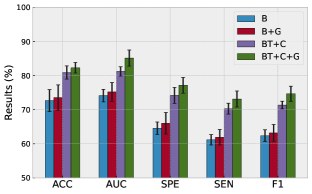
(a) ADNI-3CLS

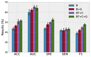
(b) ADNI-4CLS

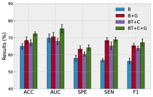
(c) ABIDE

Figure 2: Performance of MMGPL with different combination of components on all datasets, i.e., “B” denotes baseline method, “B+G” denotes baseline method with graph prompt learning, “B+C” denotes baseline method with concept learning, and “B+C+G” denotes baseline method with graph prompt learning and concept learning.

Secondly, among all methods, methods that utilize pre-trained large models (e.g., CLIP, MetaT, VPT, MaPLe, and MMGPL) outperform other methods trained directly on the dataset (e.g., ViT, BrainT, and GraphT). For example, compared to ViT, BrainT, and GraphT, MMGPL averagely improves by about 25.2% on ADNI-3CLS, 31.3% on ADNI-4CLS, and 16.5% on ABIDE, respectively. The superior performance of pre-trained models can be attributed to their exposure to a diverse range of tasks during pre-training, which enhances their ability to generalize to new tasks. This advantage is particularly beneficial when dealing with relatively small target datasets, as is frequently encountered in neurological disorder diagnosis.

Thirdly, among all methods, methods that utilize prompt learning technique (e.g., VPT, MaPLe, and MMGPL) outperform vanilla turning method on pre-trained large models (e.g., CLIP and MetaT). For example, compared to CLIP and MetaT, MMGPL averagely improves by about 24.5% on ADNI-3CLS, 11.2% on ADNI-4CLS, and 9.5% on ABIDE, respectively. The possible reason for this is that prompt learning typically involves tuning a small set of parameters that guide the model to apply its pre-learned knowledge in a specific and task-relevant manner.

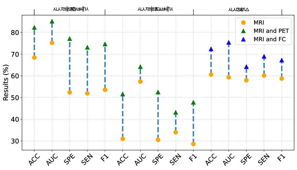
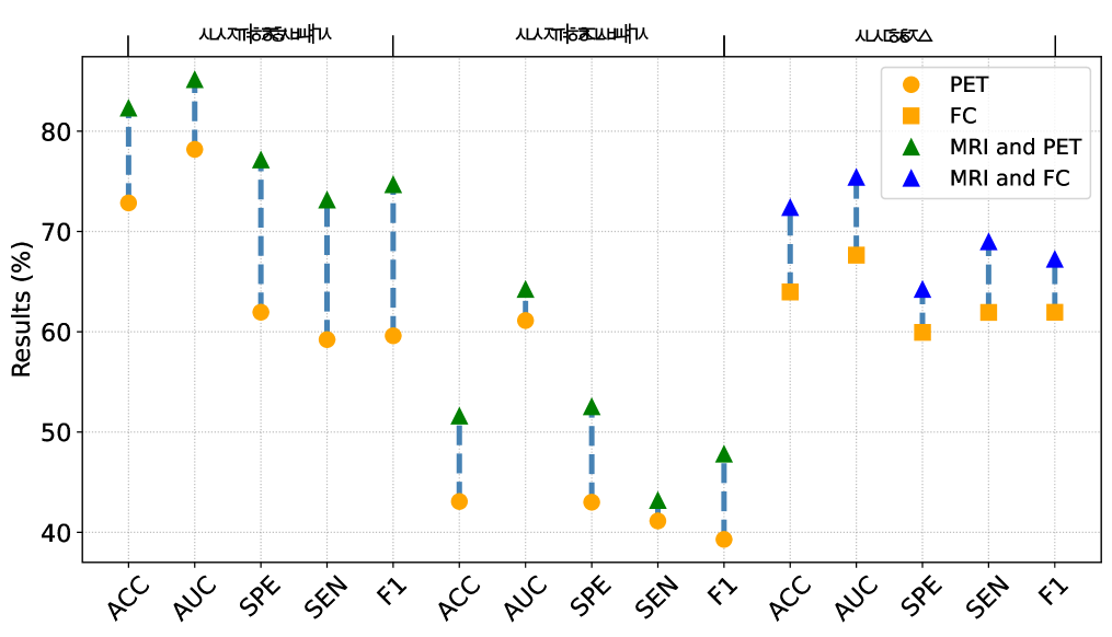
Figure 3: Performance of MMGPL with different modalities.

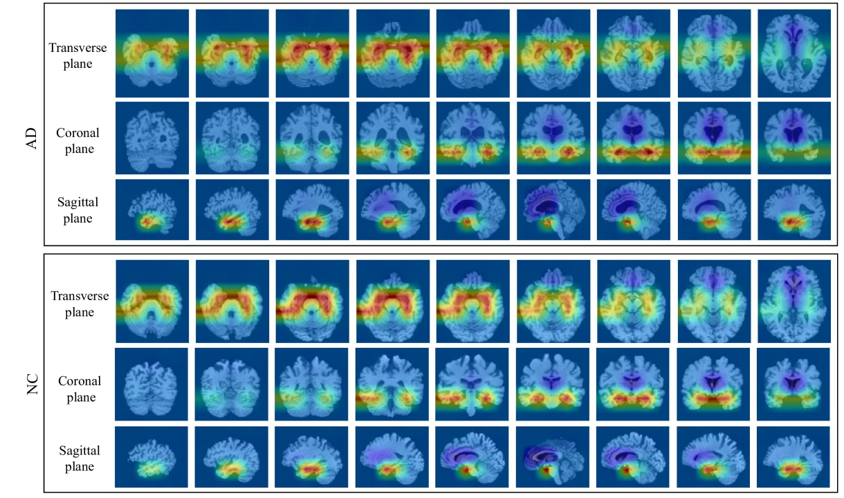
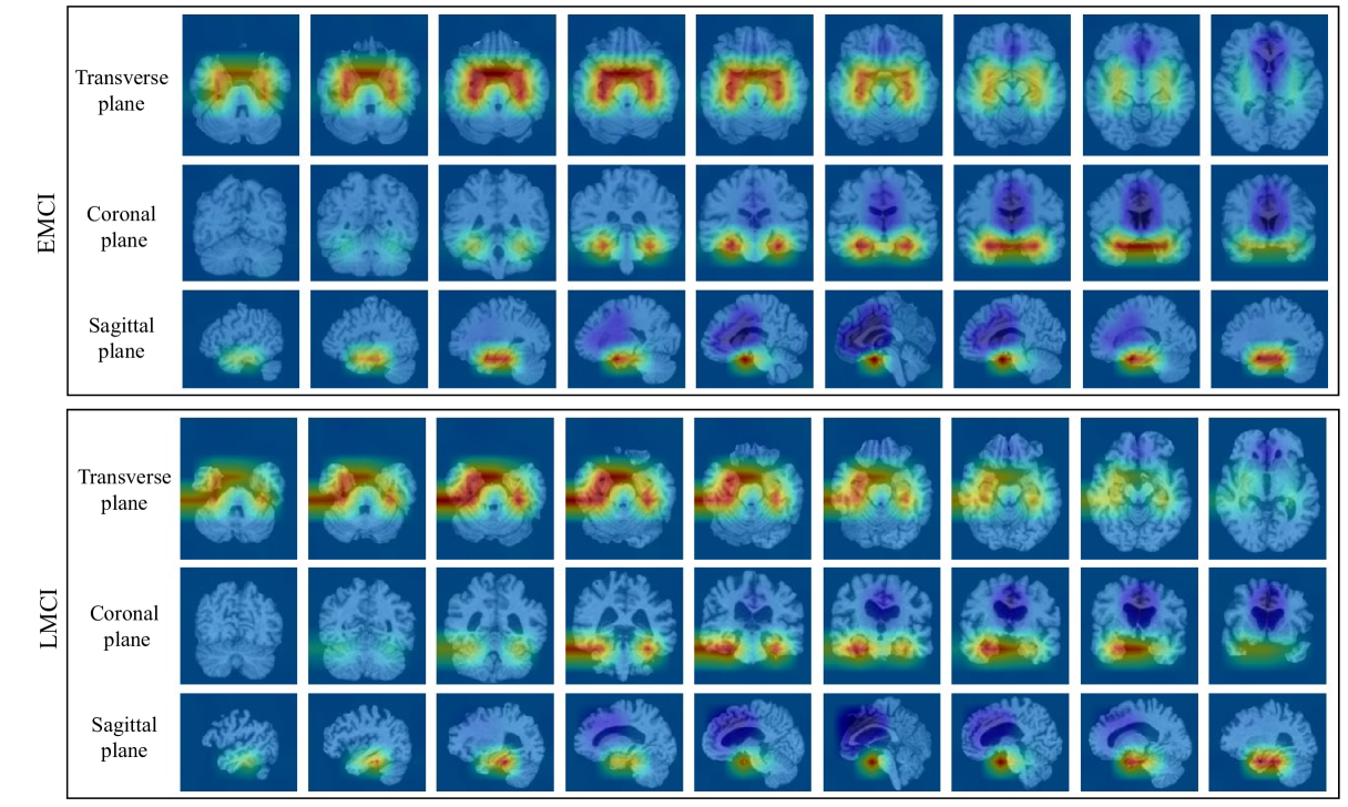
Figure 4: Heat maps generated by MMGPL on different subjects in ADNI dataset, i.e., AD (ID: 018-S-0286), NC (ID: 007-S-1222), EMCI (ID: 002-S-0729), and LMCI (ID: 002-S-0729).

IV-B2 Ablation studies

We further conduct the ablation studies with individual components and report their results in Fig. 2. Specifically, “B” denotes baseline method which apply the fine-turning strategy introduced in method MetaT (Zhang et al., 2023a). Based on this, we apply concept learning (i.e., Sec. III-C) to reduce the weights of irrelevant patches and denote as “B+C”. Similarly, we employ graph prompt learning (i.e., Sec. III-D) and denote as “B+G”. Note that, in order to ensure the proper running of the method, the semantic similarity is still need to calculated in method “B+G”. Moreover, we involve both concept learning and graph prompt learning which denotes as “B+C+G”.

Based on the experimental results, we could observe that each components has a contribution. In particular, compared to the baseline method “B”, the method “B+G” averagely improves by about 5%. Moreover, the method “B+C” markedly outperform that of the the baseline method “B”. Hence, the proposed concept learning and graph prompt learning modules have positive effect on the diagnosis of neurological disorder, which versified our claim that reduce the weight of irrelevant patches and incorporate a graph prompt making our method particularly suitable for neurological disorders diagnosis. Besides, we found that concept learning contributes more significantly to the overall performance compared to graph prompt. One possible reason is that without concept learning, the inclusion of many irrelevant tokens during graph prompt learning could have a negative impact. Considering the message propagation mechanism of GCN, these irrelevant tokens can potentially affect the graph prompt learning process and consequently affect the overall performance. Therefore, the two modules, concept learning and graph prompt learning, are closely intertwined and mutually dependent on each other.

IV-B3 Analysis

TABLE II: Comparison between MMGPL and related works on scalability. Note that, $\checkmark$(vanilla) indicates can only supports two modalities and is challenging to expand to supports more modalities.

Method	Multiple modalities	Unified model	Prompt
ViT		$\checkmark$
BrainT		$\checkmark$
GraphT	$\checkmark$(vanilla)
CLIP	$\checkmark$(vanilla)
MetaT	$\checkmark$	$\checkmark$
VPT		$\checkmark$	$\checkmark$
MaPLe	$\checkmark$(vanilla)		$\checkmark$
MMGPL	$\checkmark$	$\checkmark$	$\checkmark$

Multi-modalities. We investigate the effectiveness of individual modality and multi-modalities by reporting the performances in Fig. 2. Concretely, our method considering multi-modalities (e.g., MRI and PET in ADNI) obtains substantial improvements across all metrics, compared to only considering individual modality. This suggests that the complementary information captured by different modalities can enhance the overall performance of the model.

Interpretability. We further investigate the interpretability of our method. To achieve this, we scale the heat maps and superimpose them on the corresponding positions of the original images. The visualization of the heat map is presented in Fig. 4, with darker shades of red signifying higher weights and darker shades of blue signifying lower weights. Specifically, the x-axis represents different positions within the same plane, while the y-axis represents different planes. Firstly, it is evident that our method effectively eliminates the weights associated with almost all irrelevant patches. Secondly, Fig. 4 indicates that our method is capable of identifying the critical regions within the brain, such as hippocampal and parahippocampal. Morevoer, its interpretability has been validated by clinicians.

Scalability. We further conduct comparison between MMGPL and related works in term of scalability. As shown in Table II. we evaluate three aspects of scalability, i.e., multiple modalities, unified model, and prompt. In particular, considering the inherent multimodality of medical data, we first evaluate the model’s ability to handle multiple modalities. Note that, $\checkmark$(vanilla) indicates can only supports two modalities (e.g., image and text) and is challenging to expand to supports more modalities. Secondly, we evaluate whether the method applies a unified model for encoding multimodal medical imaging, as employing a unified model facilitates efficient inference and deployment. Thirdly, we evaluate whether the method applies prompt for fine-turning, as prompt driven fine-turning is beneficial for enhancing the interactivity and effectiveness of the method. Comparing MMGPL with all comparison methods, we can observe that our method achieve excellent scalability and flexibility.

V Conclusion

In this paper, we proposed a graph prompt learning fine-turning framework for neurological disorder diagnosis, by jointly considering the impact of irrelevant patches as well as the structural information among tokens in multimodal medical data. Specifically, we conduct concept learning, aiming to reduce weights of irrelevant tokens according to the semantic similarity between each token and disease-related concepts. Moreover, we conducted graph prompt learning with concept embeddings, aiming to bridge the gap between multimodal large models and neurological disease diagnosis. Experimental results demonstrated the effectiveness of our proposed method, compared to state-of-the-art methods on neurological disease diagnosis tasks.

References

- Belmonte et al. (2004) Belmonte, M.K., Allen, G., Beckel-Mitchener, A., Boulanger, L.M., Carper, R.A., Webb, S.J., 2004. Autism and abnormal development of brain connectivity. Journal of Neuroscience 24, 9228–9231.
- Bessadok et al. (2022) Bessadok, A., Mahjoub, M.A., Rekik, I., 2022. Graph neural networks in network neuroscience. IEEE Transactions on Pattern Analysis and Machine Intelligence 45, 5833–5848.
- Brown et al. (2020) Brown, T., Mann, B., Ryder, N., Subbiah, M., Kaplan, J.D., Dhariwal, P., Neelakantan, A., Shyam, P., Sastry, G., Askell, A., 2020. Language models are few-shot learners. Advances in neural information processing systems 33, 1877–1901.
- Bullmore and Sporns (2009) Bullmore, E., Sporns, O., 2009. Complex brain networks: graph theoretical analysis of structural and functional systems. Nature reviews neuroscience 10, 186–198.
- Cai et al. (2022) Cai, H., Gao, Y., Liu, M., 2022. Graph transformer geometric learning of brain networks using multimodal mr images for brain age estimation. IEEE Transactions on Medical Imaging 42, 456–466.
- Devlin et al. (2018) Devlin, J., Chang, M.W., Lee, K., Toutanova, K., 2018. Bert: Pre-training of deep bidirectional transformers for language understanding. arXiv preprint arXiv:1810.04805 .
- Di Martino et al. (2014) Di Martino, A., Yan, C.G., Li, Q., Denio, E., Castellanos, F.X., Alaerts, K., Anderson, J.S., Assaf, M., Bookheimer, S.Y., Dapretto, M., 2014. The autism brain imaging data exchange: towards a large-scale evaluation of the intrinsic brain architecture in autism. Molecular psychiatry 19, 659–667.
- Dinsdale et al. (2022) Dinsdale, N.K., Bluemke, E., Sundaresan, V., Jenkinson, M., Smith, S.M., Namburete, A.I., 2022. Challenges for machine learning in clinical translation of big data imaging studies. Neuron .
- Dosovitskiy et al. (2020) Dosovitskiy, A., Beyer, L., Kolesnikov, A., Weissenborn, D., Zhai, X., Unterthiner, T., Dehghani, M., Minderer, M., Heigold, G., Gelly, S., 2020. An image is worth 16x16 words: Transformers for image recognition at scale. arXiv preprint arXiv:2010.11929 .
- Driess et al. (2023) Driess, D., Xia, F., Mehdi, S., Sajjadi, C., Lynch, A., Chowdhery, B., Ichter, A., Wahid, J., Tompson, Q., Vuong, T., Yu, W., Huang, Y., Chebotar, P., Sermanet, D., Duckworth, S., Levine, V., Vanhoucke, K., Hausman, M., Toussaint, K., Greff, A., Zeng, I., Mordatch, P., Florence, 2023. Palm-e: An embodied multimodal language model arXiv:arXiv:2303.03378.
- Dvornek et al. (2019) Dvornek, N.C., Li, X., Zhuang, J., Duncan, J.S., 2019. Jointly discriminative and generative recurrent neural networks for learning from fmri, in: MLMI, Springer. pp. 382--390.
- Feigin et al. (2020) Feigin, V.L., Vos, T., Nichols, E., Owolabi, M.O., Carroll, W.M., Dichgans, M., Deuschl, G., Parmar, P., Brainin, M., Murray, C., 2020. The global burden of neurological disorders: translating evidence into policy. The Lancet Neurology 19, 255--265.
- Fornito et al. (2015) Fornito, A., Zalesky, A., Breakspear, M., 2015. The connectomics of brain disorders. Nature Reviews Neuroscience 16, 159--172.
- Gao et al. (2020) Gao, T., Fisch, A., Chen, D., 2020. Making pre-trained language models better few-shot learners. arXiv preprint arXiv:2012.15723 .
- Girdhar et al. (2023) Girdhar, R., El-Nouby, A., Liu, Z., Singh, M., Alwala, K.V., Joulin, A., Misra, I., 2023. Imagebind: One embedding space to bind them all, in: Proceedings of the IEEE/CVF Conference on Computer Vision and Pattern Recognition, pp. 15180--15190.
- Holmes et al. (1998) Holmes, C.J., Hoge, R., Collins, L., Woods, R., Toga, A.W., Evans, A.C., 1998. Enhancement of mr images using registration for signal averaging. Journal of computer assisted tomography 22, 324--333.
- Holzinger et al. (2021) Holzinger, A., Malle, B., Saranti, A., Pfeifer, B., 2021. Towards multi-modal causability with graph neural networks enabling information fusion for explainable ai. Information Fusion 71, 28--37.
- Howard and Ruder (2018) Howard, J., Ruder, S., 2018. Universal language model fine-tuning for text classification, in: Gurevych, I., Miyao, Y. (Eds.), Proceedings of the 56th Annual Meeting of the Association for Computational Linguistics (Volume 1: Long Papers), pp. 328--339. doi:10.18653/v1/P18-1031.
- Huang et al. (2023) Huang, Y., Yang, X., Liu, L., Zhou, H., Chang, A., Zhou, X., Chen, R., Yu, J., Chen, J., Chen, C., 2023. Segment anything model for medical images? arXiv preprint arXiv:2304.14660 .
- Jack Jr et al. (2008) Jack Jr, C.R., Bernstein, M.A., Fox, N.C., Thompson, P., Alexander, G., Harvey, D., Borowski, B., Britson, P.J., L. Whitwell, J., Ward, C., 2008. The alzheimer’s disease neuroimaging initiative (adni): Mri methods. Journal of Magnetic Resonance Imaging: An Official Journal of the International Society for Magnetic Resonance in Medicine 27, 685--691.
- Jaszczur et al. (2021) Jaszczur, S., Chowdhery, A., Mohiuddin, A., Kaiser, L., Gajewski, W., Michalewski, H., Kanerva, J., 2021. Sparse is enough in scaling transformers. Advances in Neural Information Processing Systems 34, 9895--9907.
- Jenkinson et al. (2002) Jenkinson, M., Bannister, P., Brady, M., Smith, S., 2002. Improved optimization for the robust and accurate linear registration and motion correction of brain images. Neuroimage 17, 825--841.
- Jenkinson et al. (2012) Jenkinson, M., Beckmann, C.F., Behrens, T.E., Woolrich, M.W., Smith, S.M., 2012. Fsl. Neuroimage 62, 782--790.
- Jia et al. (2022) Jia, M., Tang, L., Chen, B.C., Cardie, C., Belongie, S., Hariharan, B., Lim, S.N., 2022. Visual prompt tuning, in: European Conference on Computer Vision, Springer. pp. 709--727.
- Kan et al. (2022) Kan, X., Dai, W., Cui, H., Zhang, Z., Guo, Y., Yang, C., 2022. Brain network transformer. Advances in Neural Information Processing Systems 35, 25586--25599.
- Kazi et al. (2019) Kazi, A., Shekarforoush, S., Krishna, S.A., Burwinkel, H., Vivar, G., Kortüm, K., Ahmadi, S.A., Albarqouni, S., Navab, N., 2019. Inceptiongcn: receptive field aware graph convolutional network for disease prediction, in: IPMI, Springer. pp. 73--85.
- Khattak et al. (2023) Khattak, M.U., Rasheed, H., Maaz, M., Khan, S., Khan, F.S., 2023. Maple: Multi-modal prompt learning, in: Proceedings of the IEEE/CVF Conference on Computer Vision and Pattern Recognition, pp. 19113--19122.
- Kipf and Welling (2017) Kipf, T.N., Welling, M., 2017. Semi-supervised classification with graph convolutional networks, pp. 1--14.
- Kirillov et al. (2023) Kirillov, A., Mintun, E., Ravi, N., Mao, H., Rolland, C., Gustafson, L., Xiao, T., Whitehead, S., Berg, A.C., Lo, W.Y., 2023. Segment anything. arXiv preprint arXiv:2304.02643 .
- Koh et al. (2020) Koh, P.W., Nguyen, T., Tang, Y.S., Mussmann, S., Pierson, E., Kim, B., Liang, P., 2020. Concept bottleneck models, in: International conference on machine learning, PMLR. pp. 5338--5348.
- LeCun and Bengio (1995) LeCun, Y., Bengio, Y., 1995. Convolutional networks for images, speech, and time series. The handbook of brain theory and neural networks 3361, 1995.
- Lester et al. (2021) Lester, B., Al-Rfou, R., Constant, N., 2021. The power of scale for parameter-efficient prompt tuning. arXiv preprint arXiv:2104.08691 .
- Li et al. (2023) Li, C., Wong, C., Zhang, S., Usuyama, N., Liu, H., Yang, J., Naumann, T., Poon, H., Gao, J., 2023. Llava-med: Training a large language-and-vision assistant for biomedicine in one day. arXiv preprint arXiv:2306.00890 .
- Li et al. (2021) Li, X., Zhou, Y., Dvornek, N., Zhang, M., Gao, S., Zhuang, J., Scheinost, D., Staib, L.H., Ventola, P., Duncan, J.S., 2021. Braingnn: Interpretable brain graph neural network for fmri analysis. Medical Image Analysis 74, 102233.
- Li and Liang (2021) Li, X.L., Liang, P., 2021. Prefix-tuning: Optimizing continuous prompts for generation. arXiv preprint arXiv:2101.00190 .
- Liu et al. (2023) Liu, H., Li, C., Wu, Q., Lee, Y., 2023 arXiv:arXiv:2304.08485.
- Liu et al. (2022) Liu, X., Ji, K., Fu, Y., Tam, W., Du, Z., Yang, Z., Tang, J., 2022. P-tuning: Prompt tuning can be comparable to fine-tuning across scales and tasks, in: Proceedings of the 60th Annual Meeting of the Association for Computational Linguistics, pp. 61--68.
- Lord et al. (2018) Lord, C., Elsabbagh, M., Baird, G., Veenstra-Vanderweele, J., 2018. Autism spectrum disorder. The lancet 392, 508--520.
- Lu et al. (2022) Lu, Y., Liu, J., Zhang, Y., Liu, Y., Tian, X., 2022. Prompt distribution learning, in: Proceedings of the IEEE/CVF Conference on Computer Vision and Pattern Recognition, pp. 5206--5215.
- Ma and Wang (2023) Ma, J., Wang, B., 2023. Segment anything in medical images. arXiv preprint arXiv:2304.12306 .
- Maaz et al. (2023) Maaz, M., Rasheed, H., Khan, S., Khan, F.S., 2023. Video-chatgpt: Towards detailed video understanding via large vision and language models. arXiv preprint arXiv:2306.05424 .
- OpenAI (2023) OpenAI, R., 2023. Gpt-4 technical report. arxiv 2303.08774. View in Article 2, 13.
- Padurariu et al. (2012) Padurariu, M., Ciobica, A., Mavroudis, I., Fotiou, D., Baloyannis, S., 2012. Hippocampal neuronal loss in the ca1 and ca3 areas of alzheimer’s disease patients. Psychiatria Danubina 24, 152--158.
- Parisot et al. (2018) Parisot, S., Ktena, S.I., Ferrante, E., Lee, M., Guerrero, R., Glocker, B., Rueckert, D., 2018. Disease prediction using graph convolutional networks: application to autism spectrum disorder and alzheimer’s disease. Medical Image Analysis 48, 117--130.
- Pievani et al. (2014) Pievani, M., Filippini, N., Van Den Heuvel, M.P., Cappa, S.F., Frisoni, G.B., 2014. Brain connectivity in neurodegenerative diseases—from phenotype to proteinopathy. Nature Reviews Neurology 10, 620--633.
- Radford et al. (2021) Radford, A., Kim, J.W., Hallacy, C., Ramesh, A., Goh, G., Agarwal, S., Sastry, G., Askell, A., Mishkin, P., Clark, J., 2021. Learning transferable visual models from natural language supervision, in: International conference on machine learning, PMLR. pp. 8748--8763.
- Rubinov and Sporns (2010) Rubinov, M., Sporns, O., 2010. Complex network measures of brain connectivity: uses and interpretations. Neuroimage 52, 1059--1069.
- Scheltens et al. (2021) Scheltens, P., De Strooper, B., Kivipelto, M., Holstege, H., Chételat, G., Teunissen, C.E., Cummings, J., van der Flier, W.M., 2021. Alzheimer’s disease. The Lancet 397, 1577--1590.
- Schick and Schütze (2020) Schick, T., Schütze, H., 2020. Few-shot text generation with pattern-exploiting training. arXiv preprint arXiv:2012.11926 .
- Schuster and Paliwal (1997) Schuster, M., Paliwal, K.K., 1997. Bidirectional recurrent neural networks. IEEE transactions on Signal Processing 45, 2673--2681.
- Sun et al. (2020) Sun, Z., Yin, H., Chen, H., Chen, T., Cui, L., Yang, F., 2020. Disease prediction via graph neural networks. IEEE Journal of Biomedical and Health Informatics 25, 818--826.
- Tsimpoukelli et al. (2021) Tsimpoukelli, M., Menick, J., Cabi, S., Eslami, O., Vinyals, F., Hill, 2021. Multimodal few-shot learning with frozen language models arXiv:arXiv:2106.13884.
- Tu et al. (2023) Tu, T., Azizi, S., Driess, D., Schaekermann, M., Amin, M., Chang, P.C., Carroll, A., Lau, C., Tanno, R., Ktena, I., 2023. Towards generalist biomedical ai. arXiv preprint arXiv:2307.14334 .
- Vaswani et al. (2017) Vaswani, A., Shazeer, N., Parmar, N., Uszkoreit, J., Jones, L., Gomez, A.N., Kaiser, Ł., Polosukhin, I., 2017. Attention is all you need. Advances in neural information processing systems 30.
- Veličković et al. (2017) Veličković, P., Cucurull, G., Casanova, A., Romero, A., Lio, P., Bengio, Y., 2017. Graph attention networks. arXiv preprint arXiv:1710.10903 .
- Wang et al. (2023) Wang, B., Li, L., Nakashima, Y., Nagahara, H., 2023. Learning bottleneck concepts in image classification, in: Proceedings of the IEEE/CVF Conference on Computer Vision and Pattern Recognition, pp. 10962--10971.
- Wang et al. (2006) Wang, L., Zang, Y., He, Y., Liang, M., Zhang, X., Tian, L., Wu, T., Jiang, T., Li, K., 2006. Changes in hippocampal connectivity in the early stages of alzheimer’s disease: evidence from resting state fmri. Neuroimage 31, 496--504.
- Wen et al. (2020) Wen, J., Thibeau-Sutre, E., Diaz-Melo, M., Samper-González, J., Routier, A., Bottani, S., Dormont, D., Durrleman, S., Burgos, N., Colliot, O., 2020. Convolutional neural networks for classification of alzheimer’s disease: Overview and reproducible evaluation. Medical image analysis 63, 101694.
- Wingo et al. (2021) Wingo, A.P., Liu, Y., Gerasimov, E.S., Gockley, J., Logsdon, B.A., Duong, D.M., Dammer, E.B., Robins, C., Beach, T.G., M, R.E., 2021. Integrating human brain proteomes with genome-wide association data implicates new proteins in alzheimer’s disease pathogenesis. Nature genetics 53, 143--146.
- Wu et al. (2023) Wu, C., Zhang, X., Zhang, Y., Wang, Y., Xie, W., 2023. Towards generalist foundation model for radiology. arXiv preprint arXiv:2308.02463 .
- Zhang and Metaxas (2023) Zhang, S., Metaxas, D., 2023. On the challenges and perspectives of foundation models for medical image analysis. arXiv preprint arXiv:2306.05705 .
- Zhang et al. (2023a) Zhang, Y., Gong, K., Zhang, K., Li, H., Qiao, Y., Ouyang, W., Yue, X., 2023a. Meta-transformer: A unified framework for multimodal learning. arXiv preprint arXiv:2307.10802 .
- Zhang et al. (2023b) Zhang, Y., Zhou, T., Wang, S., Liang, P., Zhang, Y., Chen, D.Z., 2023b. Input augmentation with sam: Boosting medical image segmentation with segmentation foundation model, in: MICCAI, Springer. pp. 129--139.
- Zhou et al. (2022) Zhou, K., Yang, J., Loy, C.C., Liu, Z., 2022. Conditional prompt learning for vision-language models, in: Proceedings of the IEEE/CVF Conference on Computer Vision and Pattern Recognition, pp. 16816--16825.
- Zhu et al. (2022) Zhu, Y., Ma, J., Yuan, C., Zhu, X., 2022. Interpretable learning based dynamic graph convolutional networks for alzheimer’s disease analysis. Information Fusion 77, 53--61.