Semidefinite Relaxations of the Gromov-Wasserstein Distance

Abstract

The Gromov-Wasserstein (GW) distance is a variant of the optimal transport problem that allows one to match objects between incomparable spaces. At its core, the GW distance is specified as the solution of a non-convex quadratic program and is not known to be tractable to solve. In particular, existing solvers for the GW distance are only able to find locally optimal solutions. In this work, we propose a semi-definite programming (SDP) relaxation of the GW distance. The relaxation can be viewed as the dual of the GW distance augmented with constraints that relate the linear and quadratic terms of transportation maps. Our relaxation provides a principled manner to compute the approximation ratio of any transport map to the global optimal solution. Finally, our numerical experiments suggest that the proposed relaxation is strong in that it frequently computes the global optimal solution, together with a proof of global optimality.

1 Introduction

The optimal transport (OT) problem concerns the task finding a transportation plan between two probability distributions so as to minimize some cost. The problem has applications in a wide range of scientific and engineering applications. For instance, in the context of machine learning, the OT problem forms the backbone of recent breakthroughs in generative modeling [ACB17, BAMKJ19, LGL22, LCBH⁺22], natural language processing [KSKW15], domain adaptation [CFHR17].

Let $\alpha\in\Sigma_{m}$ and $\beta\in\Sigma_{m}$ be probability distributions over a metric space – here $\Sigma_{m}:=\{\alpha\in\mathbb{R}^{m}_{+},\sum_{i=1}^{m}\alpha_{i}=1\}$ denotes the probability simplex. Let $C\in\mathbb{R}^{m\times n}$ be the matrix such that $C_{i,j}$ models the transportation cost between points $x_{i}\sim\alpha$ and $y_{j}\sim\beta$. The (Kantorovich) formulation of the discrete OT problem [PC⁺19] is defined as the solution of the following convex optimization instance

$$\pi_{\mathcal{W}}\stackrel{{\scriptstyle\text{def.}}}{{=}}\operatorname*{argmin}_{\pi\in\Pi(\alpha,\beta)}\langle C,\pi\rangle.$$ (1)

Here, $\Pi(\alpha,\beta)=\{\pi\in\mathbb{R}^{m\times n}_{+}:\pi\mathbbm{1}_{n}=\alpha,\pi^{\top}\mathbbm{1}_{m}=\beta\}$ denotes the set of couplings between probability distributions $\alpha,\beta\in\Sigma_{m}$, while $\mathbbm{1}_{m}\in\mathbb{R}^{m}$ denotes the vector of ones. The OT problem (1) is an instance of a linear program (LP), and hence admits a global minimizer.

One limitation of the classical OT formulation in (1) is that the definition of the cost matrix $C$ requires the probability distributions $\alpha$ and $\beta$ to reside in the same metric space. This is problematic in application domains where we wish to compare probability distributions in different spaces, which is typical in shape comparison or graph matching, for example.

To address such scenarios, the work in [Mé11] formulates an extension of the OT problem known as the Gromov-Wasserstein (GW) distance whereby one can define an analogous OT problem given knowledge of the cost matrices for the respective spaces where $\alpha$ and $\beta$ reside in. More concretely, let the tuple $(C,\alpha)\in\mathbb{R}^{m\times m}\times\Sigma_{m}$ denote a discrete metric-measure space. Given a smooth, differentiable function $\ell:\mathbb{R}\times\mathbb{R}\to\mathbb{R}$, the Gromov-Wasserstein distance between two discrete metric-measure spaces $(C,\alpha)$ and $(D,\beta)$ is defined by

$$\text{GW}(C,D,\alpha,\beta)\stackrel{{\scriptstyle\text{def.}}}{{=}} \leavevmode\nobreak\ \leavevmode\nobreak\ \min_{\pi\in\Pi(\alpha,\beta)}\ell(C_{i,k},D_{j,l})\pi_{i,j}\pi_{k,l}$$ (GW)

$$= \leavevmode\nobreak\ \leavevmode\nobreak\ \min_{\pi\in\Pi(\alpha,\beta)}\langle\mathbf{L}(C,D)\otimes\pi,\pi\rangle.$$

Here, the transportation cost is specified by the four-way tensor that measures the discrepancy between the metrics $C$ and $D$

$$\mathbf{L}(C,D)_{i,j,k,l}\stackrel{{\scriptstyle\text{def.}}}{{=}}\ell(C_{i,k},D_{j,l}).$$ (2)

The squared loss error, for instance, is a common choice. The tensor-matrix multiplication is then defined by

$$[\mathbf{L}\otimes\pi]_{i,j}\stackrel{{\scriptstyle\text{def.}}}{{=}}\sum_{k,l}\mathbf{L}_{i,j,k,l}\pi_{k,l}.$$

The GW distance has been applied widely to machine learning tasks, most notably on graph learning [VCT⁺19, VCFC⁺22, VCVF⁺21, XLZD19]. It is an instance of a quadratic program (QP) – these are optimization instances in which we minimize a quadratic objective subject to some linear inequalities. To see this, one can re-write the objective in (GW) in terms of vectorized matrices

$$\min_{\pi}\leavevmode\nobreak\ \leavevmode\nobreak\ \langle\mathrm{vec}(\pi),L\ \mathrm{vec}(\pi)\rangle\leavevmode\nobreak\ \leavevmode\nobreak\ \mathrm{s.t.}\leavevmode\nobreak\ \leavevmode\nobreak\ \pi\in\Pi(\alpha,\beta).$$ (GW+)

Here, $(L_{ij,kl})_{ij,kl}\in\mathbb{R}^{mn\times mn}$ denotes the flattened 2-dimension tensor of $\mathbf{L}$, while the vectorization of a matrix $\pi\in\mathbb{R}^{m\times n}$ is given by

$$\mathrm{vec}(\pi)\stackrel{{\scriptstyle\text{def.}}}{{=}}[\pi_{11},\pi_{21},\dots,\pi_{m1},\dots,\pi_{mn}]^{\top}\in\mathbb{R}^{mn}.$$

The constraint $\pi\in\Pi(\alpha,\beta)$ is convex, and in fact linear. On the other hand, the matrix $L$ is usually not positive semidefinite – and this is typically the case for $L$’s arising from differences of cost matrices (2). As such, the QP instance in (GW+) is typically non-convex.

Related works. There are a number of different relaxations for solving the GW problem in the literature – in what follows, we explain the differences between these related works and ours.

First, the work in [VCT⁺19] applies an alternating minimization-type approach based on the conditional gradient (Frank-Wolfe) algorithm to find local optima to the GW problem. This algorithm is currently implemented and is the default choice within the Python Optimal Transport package [FCG⁺21]. The basic idea is to start by computing the partial derivative of the objective Equation GW with respect to $\pi$:

$$G(\pi)=2\ \mathbf{L}(C,D)\otimes\pi,$$

which in itself is a linear OT problem that can be solved using classical OT solvers. One proceeds with an alternating minimization scheme in which one updates the gradient $G$ with respect to $\pi^{(i-1)}$, subsequently solves for $\pi^{(i)}$ with the loss $G(\pi)$ at each $i$th-iteration, and finally projects $\pi^{(i)}$ into the feasible set by performing a line-search. The Conditional Gradient-based approach is not guaranteed to find globally optimal solutions; in fact, our numerical experiments in Section 5 suggest that this is quite often the case. Last, we briefly note that the work [KES21] suggests a similar alternating numerical scheme.

Second, there is a number of prior works that aim at developing numerical schemes for finding transportation plans that approximately minimize the GW objective without incurring the $O(m^{2}n^{2})$ dependency, which is a serious concern in itself. For instance, the work in [PCS16] introduces entropic regularization into the GW objective – this leads to a formulation that permits Sinkhorn scaling-like updates. The work in [VFT⁺19] adapt the ideas from the Wasserstein problem in one-dimension in which closed-form solutions are available (this known as the sliced Wasserstein problem) to the GW context. Finally, the work in [VCVF⁺21] and [SVP21] suitably relax the constraints on the probability distributions. These numerical schemes frequently lead to numerical schemes that are far more scalable than other existing methods, but they ultimately optimize for an objective that is different from the GW problem.

There is an interesting piece of work in [SPC22], which operates under the assumption that the cost matrices have low-rank structure. While the algorithm does not give guarantees about global optimality, it raises an interesting future direction; namely, could we develop numerical schemes for our proposed SDP relaxation that also exploit similar structure?

Last we discuss works that do address global optimality: One recent work is in [MN22], which suggests the use of moment sum-of-square (SOS) relaxation technique to solve the GW optimization problem. The standard SDP relaxation for QPs on which our work is based on may be viewed, in a suitable sense, as the first level of the SOS hierarchy for polynomial optimization. Unfortunately, and as we note in Section 3, this alone is insufficient – the real novelty in our work is the addition of constraints that substantially strengthen the overall convex relaxation. Another recent work by Ryner et al. [RKK23] studies the closely related Gromov-Hausdorff problem, and propose a Branch-and-Bound approach for solving integer programs. The GW problem do not contain integer constraints, and hence Branch-and-Bound techniques are not immediately applicable. That said, SDP relaxations can be used in conjunction with Branch-and-Bound! In fact, it would be interesting to see if our proposed SDP relaxations for GW suggest suitable relaxations for the Gromov-Hausdorff problem, which can be used in conjunction with the Branch-and-Bound techniques in [RKK23].

2 Main Results

The main contribution of this work is to propose a strong semidefinite programming (SDP)-based relaxation for the Gromov-Wasserstein distance that leads to globally optimal solutions in many instances. Let $(\pi_{sdp},P_{sdp})$ denote an optimal solution to the following

$$\text{GW-SDP}(C,D,\alpha,\beta)\quad\stackrel{{\scriptstyle\text{def.}}}{{=}} \min_{\begin{subarray}{c}\pi\in\mathbb{R}^{m\times n},\\ P\in\mathbb{R}^{mn\times mn}\end{subarray}}\quad\langle L,P\rangle$$ (GW-SDP)

s.t. $$\begin{pmatrix}P&\text{vec}(\pi)\\ \text{vec}(\pi)^{\top}&1\end{pmatrix}\succeq 0$$

$$\pi\in\Pi(\alpha,\beta)$$

$$P\mathrm{vec}(e_{i}\mathbbm{1}_{n}^{\top})=\alpha_{i}\text{vec}(\pi),i\in[m]$$

$$P\mathrm{vec}(\mathbbm{1}_{m}e_{j}^{\top})=\beta_{j}\text{vec}(\pi),j\in[n]$$

$$P\geq 0$$

Here, $e_{i}$ denotes the standard basis vector whose $i$-th entry is $1$.

Approximation ratios. The most valuable aspect of (GW-SDP) (as well as any other suitably defined convex relaxation) is that it provides a principled way to certify global optimality of any computed transportation map. We explain how this is done: Let $\pi^{\star}$ denote an optimal solution to (GW+), an equivalent formulation of the original GW problem. Given any transportation map $\pi\in\Pi(\alpha,\beta)$, a natural approach to quantify the quality of $\pi$ is to compare its objective value with the optimal choice:

$$\text{Apx. Ratio}(\pi)\leavevmode\nobreak\ :=\leavevmode\nobreak\ \frac{\langle\pi,\mathbf{L}\otimes\pi\rangle}{\langle\pi^{\star},\mathbf{L}\otimes\pi^{\star}\rangle}.$$

This ratio is at least one, and is equal to one if $\pi$ is also globally optimal.

Note that the optimal value of (GW-SDP) will always be a lower bound to (GW):

$$\langle\pi^{\star},\mathbf{L}\otimes\pi^{\star}\rangle=\langle\mathrm{vec}(\pi^{\star}),L\ \mathrm{vec}(\pi^{\star})\rangle\geq\langle P_{sdp},L\rangle.$$

This is because the tuple $(\pi^{\star},\mathrm{vec}(\pi^{\star})\mathrm{vec}(\pi^{\star})^{\top})$ is a feasible solution to (GW-SDP):

$$\mathrm{vec}(\pi^{\star})\mathrm{vec}(\pi^{\star})^{\top}\mathrm{vec}(e_{i}\mathbbm{1}_{m}^{\top}) =\leavevmode\nobreak\ \leavevmode\nobreak\ \mathrm{vec}(\pi^{\star})\langle\pi^{\star},e_{i}\mathbbm{1}_{m}^{\top}\rangle$$

$$=\leavevmode\nobreak\ \leavevmode\nobreak\ \mathrm{vec}(\pi^{\star})\langle\pi^{\star}\mathbbm{1}_{n},e_{i}\rangle$$

$$=\leavevmode\nobreak\ \leavevmode\nobreak\ \alpha_{i}\mathrm{vec}(\pi^{\star}).$$

(The inequalities for $\beta$ follow analogously.) Subsequently, one has

$$\text{Apx. Ratio}(\pi_{sdp})\leq\frac{\langle\pi_{sdp},\mathbf{L}\otimes\pi_{sdp}\rangle}{\langle P_{sdp},L\rangle}.$$ (3)

This bound is useful because all the quantities on the RHS can be computed efficiently as the solution of a SDP. If in fact we have an instance where the RHS evaluates to one, then we have a proof that $\pi_{sdp}$ is the global optimal solution to the GW problem. In our numerical experiments in Section 5, we observed that this is frequently the case for our experiments.

Finally, we emphasize that the SDP relaxation imposes no restriction on the cost tensor $\mathbf{L}$. This is unlike the entropic GW, which is only applicable to the cost that can be decomposed to a specific form, such as $\ell_{2}$ or discrete KL loss [PCS16].

3 SDP Relaxations Of QPs

We describe the derivation of the relaxation in (GW-SDP). The starting point is to recognize that the GW-problem is an instance of a QPs – these are optimization instances of the form

$$\begin{aligned} \min_{x\in\mathbb{R}^{n}}\quad&\quad x^{\top}Ax+2b^{\top}x+c\\ \text{s.t.}\quad&\quad Bx\leq d\end{aligned}.$$ (4)

QPs are an important class of optimization problems. If the matrix $A$ is PSD, then the objective is convex, and the QP instance can be solved tractably using standard software [NW06]. The problem becomes difficult if $A$ contains negative eigenvalues. The general class of QPs is NP-hard; for instance, it contains the problem of finding the maximum clique of a graph [MS65]. In fact, the presence of a single negative eigenvalue in $A$ is sufficient to make the class of QPs NP-hard [PV91]. The typical approach to solving a quadratic program exactly is via a branch-and-bound type of algorithm. Other approaches include relating QPs to the class of co-positive programming, mixed integer linear programmings, and deploying SDP relaxations [BdK02] – typically, these methods are used as a sub-routine within a branch-and-bound procedure.

3.1 Standard SDP Relaxation

The first step of SDP relaxation is to express the quadratic terms with a PSD matrix whose rank is one. Concretely, the QP instance (4) is equivalent to the following:

$$\begin{aligned} \min_{x\in\mathbb{R}^{n},X\in\mathbb{R}^{n\times n}}\quad&\quad\text{tr}(AX)+2b^{\top}x+c\\ \text{s.t.}\quad&\quad Bx\leq d\\ \quad&\quad\begin{pmatrix}X&x\\ x^{\top}&1\end{pmatrix}\succeq 0,\leavevmode\nobreak\ \leavevmode\nobreak\ \mathrm{rank}\begin{pmatrix}X&x\\ x^{\top}&1\end{pmatrix}=1\end{aligned}.$$

This optimization instance is not convex because of the rank-one constraint. The second step is to simply omit the rank constraint, which yields a semidefinite program, which is convex – this is the standard SDP relaxation for QPs (more generally for quadratically constrained quadratic programs (QCQPs)).

By applying the same sequence of steps to (GW+), the standard SDP relaxation one arrives at is the following:

$$\min_{\pi\in\mathbb{R}^{m\times n},P\in\mathbb{R}^{mn\times mn}} \quad\langle L,P\rangle$$ (5)

s.t. $$\quad\begin{pmatrix}P&\text{vec}(\pi)\\ \text{vec}(\pi)^{\top}&1\end{pmatrix}\succeq 0$$

$$\quad\pi\in\Pi(\alpha,\beta)$$

Problem (5) is a tractable convex semidefinite programming, which can be efficiently solved in polynomial time. If the solution to (5) (and the subsequent SDP relaxations we introduce) has rank equal to one, we would in fact have solved the original GW problem (GW). Unfortunately, the feasible region of $P$ in (5) is not compact, and the optimal value to (5) is unbounded below in general. This means that the standard SDP relaxation (5), as it stands, is ineffective.

Proposition 3.1.

The optimization instance (5) is unbounded below.

Proof.

Let $1\leq s,t\leq mn$ be coordinates such that $L_{st}>0$. Let $v:=v_{(s,t)}\in\mathbb{R}^{mn}$ be a vector whose $s$-th entry is $1$, whose $t$-th entry is $-1$, and whose remaining entries are zeros. Let $\tilde{\pi}\in\Pi(\alpha,\beta)$ be any transportation map and consider the matrix $P_{c}=\text{vec}(\tilde{\pi})\text{vec}(\tilde{\pi})^{\top}+cvv^{\top}$. Notice that $P_{c}\succeq\text{vec}(\tilde{\pi})\text{vec}(\tilde{\pi})^{\top}$ for all $c\geq 0$. Hence the choice of variables $\pi=\tilde{\pi}$ and $P=P_{c}$ are feasible. Then notice that the objective evaluates to

$$\langle L,P_{c}\rangle=\langle L,\text{vec}(\tilde{\pi})\text{vec}(\tilde{\pi})^{\top}\rangle+c(L_{ss}-2L_{st}+L_{tt})=\langle L,\text{vec}(\tilde{\pi})\text{vec}(\tilde{\pi})^{\top}\rangle-2cL_{st}.$$

We obtain the last equality by noting that $L_{ii}=0$ for all $i$ (this is a property of cost matrices). The result follows by taking $c\rightarrow+\infty$. ∎

3.2 Tightening the Relaxation

Proposition 3.1 tells us that it is necessary to augment (5) with additional constraints to further strengthen the relaxation. Ideally, we would like the optimal solution $P$ in (5) to have rank equals to one, or equivalently, $P\approx\mathrm{vec}(\pi)\mathrm{vec}(\pi)^{\top}$. To encourage such behavior, we may impose additional constraints that transportation maps $\pi\in\Pi(\alpha,\beta)$ are guaranteed to satisfy.

First, $\pi\geq 0$ for all $\pi\in\Pi(\alpha,\beta)$, and hence $\mathrm{vec}(\pi)\mathrm{vec}(\pi)^{\top}\geq 0$. Hence we may freely impose

$$P\geq 0.$$ (Nng)

Second, and as we noted earlier, the maps of the form $\mathrm{vec}(\pi)\mathrm{vec}(\pi)^{\top}$ satisfy the following equalities that relate the linear terms and quadratic terms of transportation maps:

$$P\mathrm{vec}(e_{i}\mathbbm{1}_{n}^{\top})=\alpha_{i}\text{vec}(\pi),i\in[m],$$ (Mar.)

$$P\mathrm{vec}(\mathbbm{1}_{m}e_{j}^{\top})=\beta_{j}\text{vec}(\pi),j\in[n].$$

These constraints have previously appeared in the context of solving matching problems based on a QAP instance [KKBL15, DML17]. In our context, we have chosen a slightly different formulation from that in [DML17] (in particular, incorporating (Nng)), in part based on numerical insight as to which set of constraints were most effective at promoting globally optimal solutions.

The proposed SDP relaxation (GW-SDP) is precisely (5) with the additional constraints (Nng) and (Mar.). In addition, the set of matrices $P$ satisfying (Mar.) have trace at most one. Hence the feasible region is a subset of PSD matrices with trace at most one, which is compact.

3.3 No need for rounding

We make a brief remark about rounding: The optimal solution $\hat{\pi}$ to (5) automatically satisfies $\hat{\pi}\in\Pi(\alpha,\beta)$. This means that the output map from (GW-SDP) will always be a feasible transportation map. This is actually quite different from other optimization instances in which the SDP relaxation is deployed. For instance, in the MAX-CUT problem, it is necessary to apply an additional rounding step to the SDP solution to obtain a feasible CUT of the graph [GW95, KKBL15, BLWY06].

4 Duality

Given a generic optimization instance, the dual optimization instance concerns the task of finding optimal lower bounds to the primal instance. The (Lagrangian) dual to any optimization instance is a convex program in general. As such, the process of deriving the dual to any optimization instance provides a principled way of obtaining convex relaxations of difficult optimization instances.

The objective value of the dual will always be a lower bound to the primal instance – this is precisely weak duality. In some instances, however, the objective values of these problems may coincide, and we call such settings strong duality.

In this section, we explore these relationships in the context of the GW problem. As we shall see, the proposed SDP relaxation (GW-SDP) can be viewed as being equivalent to the dual of an equivalent form of the GW problem (GW+), augmented with additional constraints that relate the linear and quadratic terms of transportation maps specified by (Nng) and (Mar.). To simplify notation, we denote

$$a_{i} \leavevmode\nobreak\ =\leavevmode\nobreak\ \mathrm{vec}(e_{i}\mathbbm{1}_{n}^{\top}),$$

$$b_{j} \leavevmode\nobreak\ =\leavevmode\nobreak\ \mathrm{vec}(\mathbbm{1}_{m}e_{j}^{\top}).$$

We proceed to describe the dual program. We start by defining the following dual variables:

$$\begin{pmatrix}Y&y\\ y^{\top}&t\end{pmatrix}\succeq 0 :\begin{pmatrix}P&\text{vec}(\pi)\\ \text{vec}(\pi)^{\top}&1\end{pmatrix}\succeq 0$$ (a)

$$\lambda_{i}\in\mathbb{R} :a_{i}^{\top}\text{vec}(\pi)=\alpha_{i},\quad i\in[m]$$ (b)

$$\mu_{j}\in\mathbb{R} :b_{j}^{\top}\text{vec}(\pi)=\beta_{j},\quad j\in[n]$$ (c)

$$Z\geq 0 :P\geq 0$$ (d)

$$\eta^{i}\in\mathbb{R}^{mn} :Pa_{i}=\alpha_{i}\text{vec}(\pi),\quad i\in[m]$$ (e)

$$\theta^{j}\in\mathbb{R}^{mn} :Pb_{j}=\beta_{j}\text{vec}(\pi),\quad j\in[n]$$ (f)

As a reminder, the constraints in (b) and (c) specify the transportation map $\Pi(\alpha,\beta)$ while the constraints in (e) and (f) correspond to (Mar.).

Theorem 4.1.

The Lagrangian dual of (GW-SDP) is given as follows

$$\max \quad\lambda^{\top}\alpha+\mu^{\top}\beta-t$$ (GW-Dual)

s.t. $$\quad\begin{pmatrix}L-Z+\frac{1}{2}\sum_{i=1}^{m}(\eta^{i}a_{i}^{\top}+a_{i}{\eta^{i}}^{\top})+\frac{1}{2}\sum_{j=1}^{n}(\theta^{j}b_{j}^{\top}+b_{j}{\theta^{j}}^{\top})&y\\ y^{\top}&t\end{pmatrix}\succeq 0,$$

$$\quad\sum_{i=1}^{m}\left(\lambda_{i}a_{i}+\alpha_{i}\eta^{i}\right)+\sum_{j=1}^{n}\left(\mu_{j}b_{j}+\beta_{j}\theta^{j}\right)+2y\leq 0,$$

$$\quad Z\geq 0.$$

Furthermore, strong duality holds; that is, the duality gap between (GW-SDP) and (GW-Dual) is zero.

It turns out that it is possible to derive the dual instance (GW-Dual) directly from (GW+), an equivalent formulation of the original GW problem, with additional constraints specified by (Nng) and (Mar.). Concretely, consider

$$\min_{\begin{subarray}{c}\pi\in\mathbb{R}^{m\times n}\\ P\in\mathbb{R}^{mn\times mn}\end{subarray}} \quad\langle L,P\rangle$$ (GW++)

s.t. $$\quad P=\text{vec}(\pi)\text{vec}(\pi)^{\top}$$

$$\quad\pi\in\Pi(\alpha,\beta)$$

$$\quad P\mathrm{vec}(e_{i}\mathbbm{1}_{n}^{\top})=\alpha_{i}\text{vec}(\pi),i\in[m]$$

$$\quad P\mathrm{vec}(\mathbbm{1}_{m}e_{j}^{\top})=\beta_{j}\text{vec}(\pi),j\in[n]$$

$$\quad P\geq 0.$$

The last three constraints on $P$ are always satisfied so long as $P=\text{vec}(\pi)\text{vec}(\pi)^{\top}$, where $\pi\in\Pi(\alpha,\beta)$ is a transportation map. Hence these constraints on $P$ and $\pi$ are technically redundant within (GW++). That is, the optimization instances (GW+) and (GW++) are equivalent. However, the Lagrangian dual of these optimization instances are different, and we summarize this observation in the following.

Theorem 4.2.

(GW-Dual) is the Lagrangian dual of (GW++).

The (duality) gap between (GW-Dual) and (GW++) is non-zero in general, and is equal to zero precisely when the convex relaxation (5) succeeds. These can be characterized by a rank condition satisfied by the optimal solutions, namely:

Proposition 4.3.

Let $P_{sdp}$ and $\pi_{sdp}$ be the solution to GW-SDP. Suppose the matrix variable has rank equals to one, that is

$$\text{rank}\begin{pmatrix}P_{sdp}&\text{vec}(\pi_{sdp})\\ \text{vec}(\pi_{sdp})^{\top}&1\end{pmatrix}=1.$$

Then the duality gap for (GW++) is zero; i.e., strong duality holds.

Proof.

The rank condition implies $P_{sdp}=\text{vec}(\pi_{sdp})\text{vec}(\pi_{sdp})^{\top}$. Subsequently, the choice of variables $\pi=\pi_{sdp}$ and $P=\text{vec}(\pi_{sdp})\text{vec}(\pi_{sdp})^{\top}$ is a feasible solution to (GW++). This means (GW++) attains the same objective value as the (GW-Dual). Recall from Theorem 4.2 that (GW-Dual) is the dual of (GW++), and hence in this instance the duality gap is indeed zero. ∎

We summarize the relationships among the original GW problem, (GW+), (GW++), (GW-SDP), and (GW-Dual) in Figure 1:

• (GW+) is an equivalent reformulation of the original GW problem.

• (GW++) is derived by introducing additional redundant constraints to (GW+). Consequently, (GW+) and (GW++) share the same optimal solutions.

• (GW-SDP) is obtained by applying the standard SDP relaxation to (GW+) and introducing supplementary constraints to tighten the relaxation.

• (GW-Dual) serves as the Lagrangian dual to both (GW++) and (GW-SDP), and strong duality establishes the equivalence between (GW-Dual) and (GW-SDP).

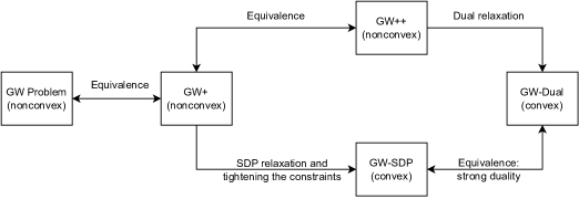
Figure 1: The relationship among the original GW problem, (GW+), (GW++), (GW-SDP) and (GW-Dual).

5 Numerical Experiments

In this section, we show the effectiveness of our proposed SDP relaxation over a range of computational tasks: transporting Gaussian distributions belonging to difference spaces, graph learning, and computing barycenters. In what follows, we will use the 2-Gromov-Wasserstein distance, i.e. the cost function is squared Euclidean norm.

We solve the GW-SDP instance implemented in CVXPY [DB16] using the SCS and MOSEK solvers [OCPB16, ApS22]. We compare our method with the Conditional Gradient solver for finding local solutions [VCT⁺19], and the Sinkhorn projections solver for computing solutions to the entropic GW problem [PCS16]. Both of the latter are implemented in Python Optimal Transport library (PythonOT [FCG⁺21]).

5.1 Matching Gaussian Distributions

In this example, we estimate the GW distance between two Gaussian point clouds, one in $\mathbb{R}^{2}$, and the other in $\mathbb{R}^{3}$. A visualization of this dataset can be found in Figure 2(a). The classical optimal transport formulation such as the likes of Wasserstein-2 distance do not apply because the two point clouds belong to different spaces.

As seen in a qualitative demonstration of Figure 2(a), our algorithm returns optimal transport plans that are as sparse as the maps obtained via the Conditional Gradient descent solver of Python OT for GW distance (CG-GW). We also vary the number of sample points and calculate the value of the objective function $\langle\pi,\mathbf{L}\otimes\pi\rangle$. As shown in Figure 3(a), the transport maps obtained by (GW-SDP) consistently returns smaller objective value (orange line) than those obtained via the GW-CG counterpart from PythonOT (blue line) and its entropic regularization (green line). This shows that the transport maps computed by PythonOT, for instance, are in fact frequently sub-optimal.

In Figure 3(b), we plot the estimated approximation ratio across different number of sample points. We notice that in this scenario of Gaussian matching, the estimated approximation ratio is close to 1.0 in most instances – this tells us that the (GW-SDP) frequently computes globally optimal transportation maps. In contrast, local methods such as PythonOT often do not.

Runtime Comparisons

Table 1 presents the run-time of the GW-SDP problem in Experiment 1, running on a PC with 8 cores CPU and 32GB of RAM. In these experiments, the cost matrix $C$ is pre-computed (i.e. assumed given). As such, the run-time is independent of data dimension. The GW-SDP has a matrix of dimension $mn\times mn$, which is slower than most local and entropic solvers. However, the solvers we implement (SCS and MOSEK) are off-the-shelf and are general SDP solvers that do not exploit special structure in the problem, and do not provide options to use initialization of the transport plans. (SCS is a first-order method, but we are otherwise unaware of its complexity). We would like to emphasize that in most settings where SDPs are applied, one will always try to develop specialized solvers that exploit structure in the problem. In our set-up, the optimal solution has low-rank, and is rank-one if the relaxation is tight. There are numerous well established methods for exploiting such structure, a point we note in the main text. This is the subject of on-going work.

Table 1: Average run time (in seconds) for Experiment 1 (matching Gaussians) with varying number of samples $n$.

	$n=6$	$n=12$	$n=20$
GW-SDP	0.2437 (0.0265)	11.615 (2.4088)	216.3645 (14.1123)
GW-CG	0.0005 (0.000041)	0.0006 (0.00003)	0.0014 (0.000017)
eGW	0.226 (0.1145)	0.2596 (0.0726)	0.4923 (0.1500)

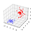
(a) Datasets visualization

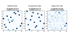
(b) Solution of the OT plans

Figure 2: Left: source distribution (2D, blue dots) and target distribution (3D, red dots). For ease of visualization, we lift the source $\mathbb{R}^{2}$ mm-spaces into target $\mathbb{R}^{3}$ by padding the third coordinate to zero. Right: OT solutions of GW-SDP (our algorithm), CG-GW (conditional gradient descent, default solver of PythonOT) and entropic OT solver. The OT plans from GW-SDP is almost sparse in the same manner to CG-GW, while the eGW is not.

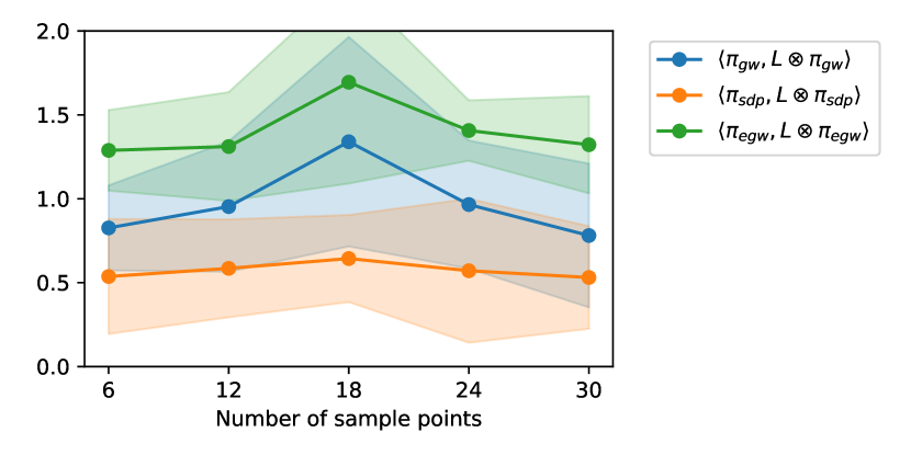
(a) Objective of problem Equation GW-SDP.

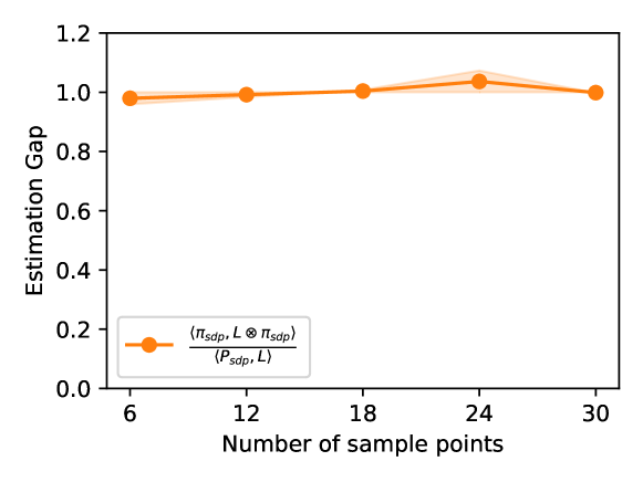
(b) Estimation gap (RHS of Equation 3).

Figure 3: Value of the objective (upper) and estimation gap (lower) with varying number of sample points, calculated on 10 runs of the Gaussian matching experiment.

5.2 Graph Community Matching

The objective of this task is to find a matching between two random graphs that are drawn from the stochastic block model (SBM, [HLL83, Abb17]) with fixed inter/intra-clusters probability (the probability that nodes inside and outside a cluster connect to each other, respectively.). The source is a three-cluster SBM whose intra-cluster probability is $p=\{1.0,0.95,0.9\}$, and the target is a two-cluster SBM whose intra-cluster probability is $p=\{1.0,0.9\}$. The inter-clusters probability are all set to 0.1. The distance matrices on each graph is created first by simulating the node features drawn from Gaussian distributions with uniform weights. Subsequently, we compute the $\ell_{2}$ norm between nodes, and shrink the value of disconnected nodes to zero to form the distance matrices.

We compare the transportation maps obtained using our methods with the baseline comparisons GW-CG and eGW in Figure 4(a). We note that the (GW-SDP) model typically returns a transport plan with a smaller total transportation cost (i.e., a smaller objective value) $\langle\pi_{sdp},\mathbf{L}\otimes\pi_{sdp}\rangle$. This trend is consistent with our observations in the previous experiment. Nevertheless, we see a degree of similarity between the transportation maps provided as output by all three methods. In addition, the maps computed by our method and GW-CG are both reasonably sparse.

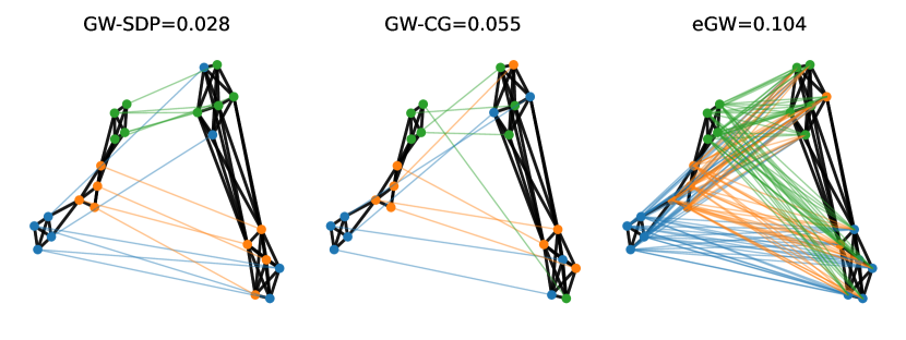
(a) Matching with GW.

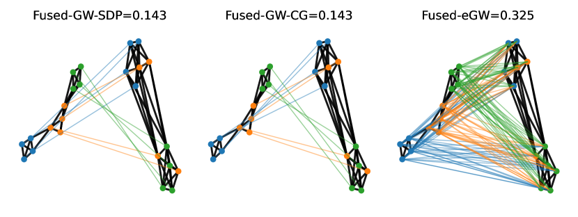
(b) Matching with FGW.

Figure 4: Value of the objective on the synthetic graph matching task, from the three-block SBM (left) to the two-block SBM (right). Upper: calculated using GW. Lower: calculated using Fused-GW.

5.3 GW-SDP Barycenters

One popular application of optimal transport is to compute the barycenters of measures that serves as a building block for many learning methods. The notion of barycenter for measures was first proposed in [AC11] for Wasserstein space. Akin to barycenter in Euclidean space (Fréchet), the Wasserstein barycenter is defined as the solution of a weighted sum of OT distances over the space of measures. An efficient algorithm to compute the discrete OT barycenter with entropic regularization was proposed in [BCC⁺15], and was later extended to discrete metric-measure spaces with entropic GW distance in [PCS16].

We show that it is straightforward to extend the GW-SDP formulation to find barycenters of a set of data as Fréchet means. For simplicity, we assume that the base histogram $\bar{\alpha}$, the size of the barycenters $m\in\mathbb{N}$, and $(\lambda_{k})_{k}$ such that $\sum_{k}\lambda_{k}=1$ are fixed. Our aim is to find a structure matrix $\bar{C}$ that minimizes

$$\min\sum_{k}\lambda_{k}\text{GW-SDP}(C_{k},\bar{C},\alpha_{k},\bar{\alpha}).$$ (6)

We have the following corollary.

Corollary 5.1 (Adaptation of Proposition 3 in [PCS16]).

In the special case of the squared loss $\ell(a,b)=(a-b)^{2}$, the solution of (6) reads

$$\bar{C}=\frac{\sum_{k}\lambda_{k}\pi^{\top}_{sdp,k}C_{k}\pi_{sdp,k}}{\alpha\alpha^{\top}},$$ (7)

where $\pi_{sdp,k}$ is the solution to GW-SDP$(C_{k},\bar{C},\alpha_{k},\bar{\alpha})$ and the division is entry-wise.

Corollary 5.1 shows that we may apply iterative updates to solve for the barycenter $\bar{C}$ via the Block Coordinate Descent (BCD) algorithm. At each iteration, we solve $K$ independent instances of the GW-SDP problem to find $(\pi_{sdp,k})_{k}$, and then compute $\bar{C}$ using (7) to solve for (6). A pseudocode for the GW-SDP barycenter calculation is provided in Algorithm 1. We demonstrate the effectiveness of the GW-SDP barycenter calculation by applying it to find the barycenter of a graph dataset. The dataset consists of 20 noisy graphs by adding random connections from a circular graph. We show a visualization of 9 of these in Figure 5(a). The number of nodes ranges from 8-16. We apply the (GW-SDP) barycenters update for 100 iterations, and Figure 5(b) shows the result for a circular graph of 10 nodes.

Algorithm 1 Computation of GW-SDP barycenters.

  Input: dataset $\{C_{k},\alpha_{k}\}_{k=1}^{K}$; $\{\lambda_{k}\}_{k=1}^{K}$.

  Initialize $\bar{C}$.

  repeat

     for $k=1$ to $K$ do

        $\pi_{sdp,k}\leftarrow$ solve_GW-SDP$(C_{k},\bar{C},\alpha_{k},\bar{\alpha})$.

     end for

     Update $\bar{C}$ using Equation 7.

  until convergence

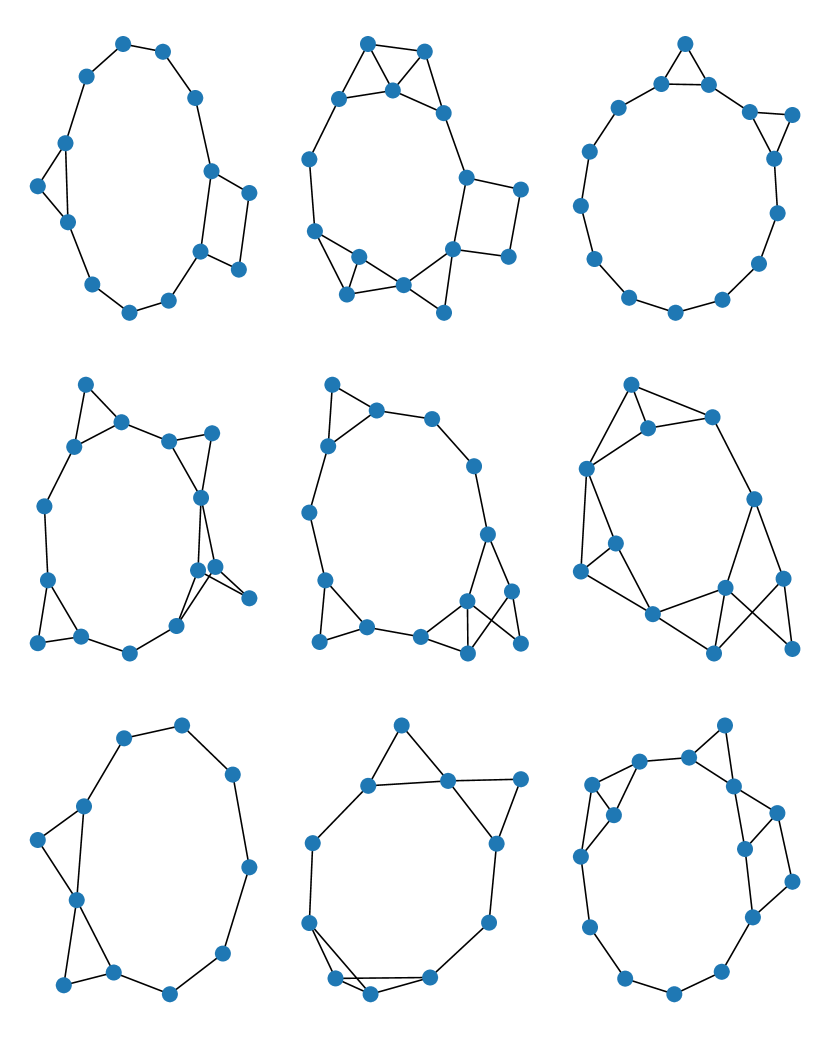
(a) Visualization of noisy circular graphs.

(b) Graph barycenter learned by (GW-SDP).

Figure 5: Application of the (GW-SDP) to find graph barycenter of noisy circular graphs.

5.4 Extension of GW-SDP to Structured Data

In this example, we consider an extension of the (GW-SDP) to structured data, more specifically graph with node features similar to the Fused-GW distance in [VCT⁺19]. The discrete metric-measure space is now described by the tuple $(F,C,\alpha)\in\mathbb{R}^{m\times d}\times\mathbb{R}^{m\times m}\times\Sigma_{m}$, where $F\stackrel{{\scriptstyle\text{def.}}}{{=}}(f_{i})_{i}\in\mathbb{R}^{d}$ encodes the feature information of the sample point. The Fused GW-SDP (FGW-SDP) formulation is given by

FGW-SDP $$(M_{FG},C,D,\alpha,\beta,\xi)$$ (FGW-SDP)

$$\stackrel{{\scriptstyle\text{def.}}}{{=}}\min_{\begin{subarray}{c}\pi\in\mathbb{R}^{m\times n},\\ P\in\mathbb{R}^{mn\times mn}\end{subarray}} (1-\xi)\langle M_{\alpha,\beta},\pi\rangle+\xi\langle L,P\rangle$$

s.t. $$\begin{pmatrix}P&\text{vec}(\pi)\\ \text{vec}(\pi)^{\top}&1\end{pmatrix}\succeq 0$$

$$\pi\in\Pi(\alpha,\beta)$$

$$P\mathrm{vec}(e_{i}\mathbbm{1}_{n}^{\top})=\alpha_{i}\text{vec}(\pi),i\in[m]$$

$$P\mathrm{vec}(\mathbbm{1}_{m}e_{j}^{\top})=\beta_{j}\text{vec}(\pi),j\in[n]$$

$$P\geq 0,$$

with $M_{FG}=d(f_{j},g_{j})_{i,j}$ encodes the distance between node features, and $\xi\in[0,1]$ the interpolation parameter. Figure 4(b) shows the result of matching two SBM graphs with the same setting as in Section 5.2, with the exception that now we input the feature to calculate $M_{FG}$ by $\ell_{2}$ norm, and the structured matrices are shortest path matrices obtained from the adjacency matrices of the graphs. We set $\xi=0.8$ for this example. The figure shows that the output OT plans and values of (FGW-SDP) and FGW-CG (using PythonOT) are identical, while entropic Fused-GW returned higher value and a denser transport plan. This indicates that SDP relaxation of Fused-GW can be useful in graph matching applications, akin to Fused-GW.

6 Conclusions and Future Directions

In this work, we proposed a semidefinite programming relaxation of the Gromov-Wasserstein distance. Our initial results suggest that the relaxation (GW-SDP) is strong in the sense that $\pi_{sdp}$ frequently coincides with the global optimal solution; moreover, we are able to provide a proof when this actually happens. These results are exciting, as it suggests a tractable approach for solving the GW-problem – at least for examples of interest – which was previously assumed to be quite difficult.

An interesting future direction is to understand precisely how difficult is an instance of the GW-problem. The GW-problem is a non-convex QP, but beyond this, little is known about its difficulty. The fact that our convex relaxations work very well for the examples we considered suggests that the GW-problem might not be as difficult as we think. It is important to bear in mind that these cost tensors $\mathbf{L}$ have structure – they arise from the difference of actual cost matrices. Could it be that the difficult instances of the GW-problem correspond to cost tensors $\mathbf{L}$ that are not realizable as the difference of cost matrices; e.g., they violate the triangle inequality? A concrete question to this end is: Is the GW problem corresponding to cost tensors $\mathbf{L}$ arising in practical instances tractable to solve?

A second important future direction concerns computation. One limitation of our proposed convex relaxation is that it is specified as the solution of a SDP in which the matrix dimension is $mn$; that is, it is equal to the dimension of the transport map. The prohibitive dependence on the data dimension means that we are currently only able to apply the relaxation on moderate sized instances using off-the-shelf SDP solvers. It would be of interest to develop specialized algorithms to solve the proposed relaxation (GW-SDP).

Appendix A Proofs of Duality Statements

We begin by defining these functions:

$$H(\eta,\theta,Z)\leavevmode\nobreak\ \leavevmode\nobreak :=\leavevmode\nobreak\ \leavevmode\nobreak\ L-Z+\frac{1}{2}\sum_{i=1}^{m}(\eta^{i}a_{i}^{\top}+a_{i}{\eta^{i}}^{\top})+\frac{1}{2}\sum_{j=1}^{n}(\theta^{j}b_{j}^{\top}+b_{j}{\theta^{j}}^{\top}),$$

$$g(\lambda,\mu,\eta,\theta,y)\leavevmode\nobreak\ \leavevmode\nobreak :=\leavevmode\nobreak\ \leavevmode\nobreak\ \sum_{i=1}^{m}\left(\lambda_{i}a_{i}+\alpha_{i}\eta^{i}\right)+\sum_{j=1}^{n}\left(\mu_{j}b_{j}+\beta_{j}\theta^{j}\right)+2y.$$

Proof of Theorem 4.1.

[Deriving the dual program]: The dual function of the GW-SDP problem is given by

$$\min_{P,\pi\geq 0} \leavevmode\nobreak\ \leavevmode\nobreak\ \text{tr}(LP)-\text{tr}(YP)-2y^{\top}\text{vec}(\pi)-t$$

$$\quad+\sum_{i=1}^{m}\lambda_{i}(\alpha_{i}-a_{i}^{\top}\text{vec}(\pi))+\sum_{j=1}^{n}\mu_{j}(\beta_{j}-b_{j}^{\top}\text{vec}(\pi))$$

$$\quad+\sum_{i=1}^{m}{\eta^{i}}^{\top}\left(Pa_{i}-\alpha_{i}\text{vec}(\pi)\right)+\sum_{j=1}^{n}{\theta^{j}}^{\top}\left(Pb_{j}-\beta_{j}\text{vec}(\pi)\right)$$

$$\quad-\text{tr}(ZP)$$

$$=\leavevmode\nobreak\ \leavevmode\nobreak\ \min_{P} \leavevmode\nobreak\ \leavevmode\nobreak\ \mathrm{tr}\left(\left(H(\eta,\theta,Z)-Y\right)P\right)\leavevmode\nobreak\ \leavevmode\nobreak\ +\leavevmode\nobreak\ \leavevmode\nobreak\ \min_{\pi\geq 0}\leavevmode\nobreak\ \leavevmode\nobreak\ \left\langle-g(\lambda,\mu,\eta,\theta,y),\text{vec}(\pi)\right\rangle$$

$$\quad+\lambda^{\top}\alpha+\mu^{\top}\beta-t.$$

In the above minimization over $P$, we observe that the objective evaluates to $-\infty$ if the following does not hold

$$H(\eta,\theta,Z)=Y.$$

Similarly, in the minimization over $\pi\geq 0$, the objective evaluates to $-\infty$ if the following does not hold

$$g(\lambda,\mu,\eta,\theta,y)\leq 0.$$

We impose these as constraints, and we add the additional constraint that $Y\succeq 0$ on our dual variable, to obtain the form of the dual problem in (GW-Dual).

[Establishing zero duality gap]: Notice that (GW-SDP) and (GW-Dual) are convex programs. Hence, to show strong duality, it suffices to check that Slater’s condition hold; that is, there exists a strictly feasible solution.

Consider $\eta^{i}=(|\lambda_{\rm min}(L)|+2)\mathbbm{1}$, $\lambda_{i}=-2m$ for $i\in[m]$, $\theta^{j}=0$, $\mu_{j}=0$ for $j\in[n]$, $t=1$, $y=0$, and

$$Z=(|\lambda_{\rm min}(L)|+2)\mathbbm{1}\mathbbm{1}^{\top}-(|\lambda_{\rm min}(L)|+1)I$$

for some $\mathbbm{1}$, $0$ and $I$ of appropriate dimension. Then we have $Z>0$, and

$$g(\lambda,\mu,\eta,\theta,y)=-2m\sum_{i=1}^{m}a_{i}+\sum_{i=1}^{m}\mathbbm{1}=-m\mathbbm{1}<0.$$

Additionally, since $H(\eta,\theta,Z)=L+(|\lambda_{\rm min}(L)|+1)I\succ 0$, $t>0$ and $y=0$, it follows that the LHS of the first constraint in (GW-Dual) is positive definite. Therefore, we find a feasible solution of (GW-Dual) such that strict inequality holds for all inequality constraints. Strong duality then follows. ∎

Proof of Theorem 4.2.

In addition to the dual variables (b)-(f), we define these additional dual variables:

$$Y\in\mathbb{R}^{mn\times mn} :P=\text{vec}(\pi)\text{vec}(\pi)^{\top}$$

$$z\geq 0 :\text{vec}(\pi)\geq 0$$

Then the dual function of (GW++) is given by

$$\min_{\pi,P}\text{tr}(LP)-\text{tr}(Y(P-\text{vec}(\pi)\text{vec}(\pi)^{\top}))+\sum_{i=1}^{m}\lambda_{i}(\alpha_{i}-a_{i}^{\top}\text{vec}(\pi))+\sum_{j=1}^{n}\mu_{j}(\beta_{j}-b_{j}^{\top}\text{vec}(\pi))$$

$$\quad+\sum_{i=1}^{m}{\eta^{i}}^{\top}\left(Pa_{i}-\alpha_{i}\text{vec}(\pi)\right)+\sum_{j=1}^{n}{\theta^{j}}^{\top}\left(Pb_{j}-\beta_{j}\text{vec}(\pi)\right)-\text{tr}(ZP)-z^{\top}\text{vec}(\pi)$$

$$=\leavevmode\nobreak\ \leavevmode\nobreak\ \min_{P}\leavevmode\nobreak\ \leavevmode\nobreak\ \underbrace{\text{tr}(\left(H(\eta,\theta,Z)-Y\right)P)}_{A_{1}}$$

$$\quad+\min_{\pi}\leavevmode\nobreak\ \leavevmode\nobreak\ \underbrace{\text{vec}(\pi)^{\top}Y\text{vec}(\pi)-\left(\sum_{i=1}^{m}(\lambda_{i}a_{i}+\alpha_{i}\eta^{i})+\sum_{j=1}^{n}(\mu_{j}b_{j}+\beta_{j}\theta^{j})+z\right)^{\top}\text{vec}(\pi)}_{A_{2}}$$

$$\quad+\lambda^{\top}\alpha+\mu^{\top}\beta.$$

To simplify notation, we denote

$$p:=\sum_{i=1}^{m}(\lambda_{i}a_{i}+\alpha_{i}\eta^{i})+\sum_{j=1}^{n}(\mu_{j}b_{j}+\beta_{j}\theta^{j}).$$

Observe that

$$\min_{P\in\mathbb{R}^{mn\times mn}}A_{1}=\begin{cases}0&,\quad\text{if $Y=H(\eta,\theta,Z)$}\\ -\infty&,\quad\text{otherwise}\end{cases},$$

and

$$\max_{\pi\in\mathbb{R}^{m\times n}}A_{2}=\begin{cases}-\frac{1}{4}(p+z)^{\top}Y^{\dagger}(p+z)&,\quad\text{if $Y\succeq 0$ and $(I-YY^{\dagger})(p+z)=0$}\\ -\infty&,\quad\text{otherwise}\end{cases}$$

Hence, the dual of (GW++) is given by

$$\begin{aligned} \max_{\lambda,\mu,y,z,Z}\quad&\quad\lambda^{\top}\alpha+\mu^{\top}\beta-\frac{1}{4}(p+z)^{\top}Y^{\dagger}(p+z)\\ \text{s.t.}\quad&\quad Y\succeq 0\\ &\quad(I-YY^{\dagger})(p+z)=0\\ &\quad Y=H(\eta,\theta,Z)\\ &\quad Z\geq 0\\ &\quad z\geq 0\end{aligned}.$$

We re-write this as

$$\max_{\lambda,\mu,y,z,Z,t} \quad\lambda^{\top}\alpha+\mu^{\top}\beta-t$$

s.t. $$\quad\frac{1}{4}(p+z)^{\top}Y^{\dagger}(p+z)\leq t$$

$$\quad Y\succeq 0$$

$$\quad(I-YY^{\dagger})(p+z)=0$$

$$\quad Y=H(\eta,\theta,Z)$$

$$\quad Z\geq 0$$

$$\quad z\geq 0$$

By taking Schur complements and by replacing $Y$ with $H(\eta,\theta,Z)$, the above optimization instance reduces to

$$\max_{\lambda,\mu,z,Z,t} \quad\lambda^{\top}\alpha+\mu^{\top}\beta-t$$

s.t. $$\quad\begin{pmatrix}H(\eta,\theta,Z)&-\frac{1}{2}(p+z)\\ -\frac{1}{2}(p+z)^{\top}&t\end{pmatrix}\succeq 0$$

$$\quad Z\geq 0$$

$$\quad z\geq 0$$

Note that $g(\lambda,\mu,\eta,\theta,y)=p+2y$, the theorem then follows by doing a change of variable $y=-\frac{1}{2}(p+z)$. ∎

References

- [Abb17] E. Abbe. Community detection and stochastic block models: recent developments. The Journal of Machine Learning Research, 18(1):6446–6531, 2017.
- [AC11] M. Agueh and G. Carlier. Barycenters in the Wasserstein space. SIAM Journal on Mathematical Analysis, 43(2):904–924, 2011.
- [ACB17] M. Arjovsky, S. Chintala, and L. Bottou. Wasserstein Generative Adversarial Networks. In D. Precup and Y. W. Teh, editors, Proceedings of the 34th International Conference on Machine Learning, volume 70 of Proceedings of Machine Learning Research, pages 214–223. PMLR, 06–11 Aug 2017.
- [ApS22] M. ApS. The MOSEK optimization toolbox for Python manual. Version 10.0., 2022.
- [BAMKJ19] C. Bunne, D. Alvarez-Melis, A. Krause, and S. Jegelka. Learning generative models across incomparable spaces. In International conference on machine learning, pages 851–861. PMLR, 2019.
- [BCC+15] J.-D. Benamou, G. Carlier, M. Cuturi, L. Nenna, and G. Peyré. Iterative Bregman projections for regularized transportation problems. SIAM Journal on Scientific Computing, 37(2):A1111–A1138, 2015.
- [BdK02] I. M. Bomze and E. de Klerk. Solving standard quadratic optimization problems via linear, semidefinite and copositive programming. J. Global Optim., 24(2):163–185, 2002.
- [BLWY06] P. Biswas, T.-C. Lian, T.-C. Wang, and Y. Ye. Semidefinite programming based algorithms for sensor network localization. ACM Transactions on Sensor Networks (TOSN), 2(2):188–220, 2006.
- [CFHR17] N. Courty, R. Flamary, A. Habrard, and A. Rakotomamonjy. Joint distribution optimal transportation for domain adaptation. Advances in neural information processing systems, 30, 2017.
- [DB16] S. Diamond and S. Boyd. CVXPY: A Python-embedded modeling language for convex optimization. Journal of Machine Learning Research, 17(83):1–5, 2016.
- [DML17] N. Dym, H. Maron, and Y. Lipman. DS++: A Flexible, Scalable and Provably Tight Relaxation for Matching Problems. ACM Transactions on Graphics, 36(184):1–14, 2017.
- [FCG+21] R. Flamary, N. Courty, A. Gramfort, M. Z. Alaya, A. Boisbunon, S. Chambon, L. Chapel, A. Corenflos, K. Fatras, N. Fournier, L. Gautheron, N. T. Gayraud, H. Janati, A. Rakotomamonjy, I. Redko, A. Rolet, A. Schutz, V. Seguy, D. J. Sutherland, R. Tavenard, A. Tong, and T. Vayer. POT: Python Optimal Transport. Journal of Machine Learning Research, 22(78):1–8, 2021.
- [GW95] M. X. Goemans and D. P. Williamson. Improved approximation algorithms for maximum cut and satisfiability problems using semidefinite programming. Journal of the ACM (JACM), 42(6):1115–1145, 1995.
- [HLL83] P. W. Holland, K. B. Laskey, and S. Leinhardt. Stochastic blockmodels: First steps. Social networks, 5(2):109–137, 1983.
- [KES21] T. Kerdoncuff, R. Emonet, and M. Sebban. Sampled Gromov Wasserstein. Machine Learning, 110(8):2151–2186, 2021.
- [KKBL15] I. Kezurer, S. Z. Kovalsky, R. Basri, and Y. Lipman. Tight relaxation of quadratic matching. In Computer graphics forum, volume 34, pages 115–128. Wiley Online Library, 2015.
- [KSKW15] M. Kusner, Y. Sun, N. Kolkin, and K. Weinberger. From Word Embeddings To Document Distances. In F. Bach and D. Blei, editors, Proceedings of the 32nd International Conference on Machine Learning, volume 37 of Proceedings of Machine Learning Research, pages 957–966, Lille, France, 07–09 Jul 2015. PMLR.
- [LCBH+22] Y. Lipman, R. T. Chen, H. Ben-Hamu, M. Nickel, and M. Le. Flow matching for generative modeling. arXiv preprint arXiv:2210.02747, 2022.
- [LGL22] X. Liu, C. Gong, and Q. Liu. Flow straight and fast: Learning to generate and transfer data with rectified flow. arXiv preprint arXiv:2209.03003, 2022.
- [MN22] O. Mula and A. Nouy. Moment-SoS Methods for Optimal Transport Problems. arXiv preprint arXiv:2211.10742, 2022.
- [MS65] T. Motzkin and E. G. Straus. Maxima for graphs and a new proof of a theorem of Tur´an. Canadian Journal of Mathematics, 1965.
- [Mé11] F. Mémoli. Gromov–Wasserstein Distances and the Metric Approach to Object Matching. Foundations of Computational Mathematics, 11(4):417–487, August 2011.
- [NW06] J. Nocedal and S. J. Wright. Numerical Optimization. Springer, 2006.
- [OCPB16] B. O’Donoghue, E. Chu, N. Parikh, and S. Boyd. Conic Optimization via Operator Splitting and Homogeneous Self-Dual Embedding. Journal of Optimization Theory and Applications, 169(3):1042–1068, June 2016.
- [PC+19] G. Peyré, M. Cuturi, et al. Computational optimal transport: With applications to data science. Foundations and Trends® in Machine Learning, 11(5-6):355–607, 2019.
- [PCS16] G. Peyré, M. Cuturi, and J. Solomon. Gromov-wasserstein averaging of kernel and distance matrices. In International conference on machine learning, pages 2664–2672. PMLR, 2016.
- [PV91] P. M. Pardalos and S. A. Vavasis. Quadratic programming with one negative eigenvalue is NP-hard. Journal of Global optimization, 1(1):15–22, 1991.
- [RKK23] M. Ryner, J. Kronqvist, and J. Karlsson. Globally solving the Gromov-Wasserstein problem for point clouds in low dimensional Euclidean spaces. arXiv preprint arXiv:2307.09057, 2023.
- [SPC22] M. Scetbon, G. Peyré, and M. Cuturi. Linear-time gromov wasserstein distances using low rank couplings and costs. In International Conference on Machine Learning, pages 19347–19365. PMLR, 2022.
- [SVP21] T. Sejourne, F.-X. Vialard, and G. Peyré. The Unbalanced Gromov Wasserstein Distance: Conic Formulation and Relaxation. In Advances in Neural Information Processing Systems, volume 34, pages 8766–8779, 2021.
- [VCFC+22] C. Vincent-Cuaz, R. Flamary, M. Corneli, T. Vayer, and N. Courty. Template based Graph Neural Network with Optimal Transport Distances. In S. Koyejo, S. Mohamed, A. Agarwal, D. Belgrave, K. Cho, and A. Oh, editors, Advances in Neural Information Processing Systems, volume 35, pages 11800–11814. Curran Associates, Inc., 2022.
- [VCT+19] T. Vayer, N. Courty, R. Tavenard, C. Laetitia, and R. Flamary. Optimal Transport for structured data with application on graphs. In K. Chaudhuri and R. Salakhutdinov, editors, Proceedings of the 36th International Conference on Machine Learning, volume 97 of Proceedings of Machine Learning Research, pages 6275–6284. PMLR, 09–15 Jun 2019.
- [VCVF+21] C. Vincent-Cuaz, T. Vayer, R. Flamary, M. Corneli, and N. Courty. Online Graph Dictionary Learning. In M. Meila and T. Zhang, editors, Proceedings of the 38th International Conference on Machine Learning, volume 139 of Proceedings of Machine Learning Research, pages 10564–10574. PMLR, 18–24 Jul 2021.
- [VFT+19] T. Vayer, R. Flamary, R. Tavenard, L. Chapel, and N. Courty. Sliced Gromov-Wasserstein. In Advances in Neural Information Processing Systems, volume 33, pages 14753–14763, 2019.
- [XLZD19] H. Xu, D. Luo, H. Zha, and L. C. Duke. Gromov-Wasserstein Learning for Graph Matching and Node Embedding. In K. Chaudhuri and R. Salakhutdinov, editors, Proceedings of the 36th International Conference on Machine Learning, volume 97 of Proceedings of Machine Learning Research, pages 6932–6941. PMLR, 09–15 Jun 2019.