Machine learning for structure-guided materials and process design
Abstract
In recent years, there has been a growing interest in accelerated materials innovation in both, research and industry. However, to truly add value to the development of new advanced materials, it is inevitable to take into account manufacturing processes and thereby tailor materials design approaches to support downstream process design approaches. As a major step into this direction, we present a holistic optimization approach that covers the entire materials process-structure-property chain. Our approach specifically employs machine learning techniques to address two critical identification problems. The first is to solve a materials design problem, which involves identifying near-optimal material structures that exhibit desired macroscopic properties. The second is to solve a process design problem that is to find an optimal processing path to manufacture these material structures. Both identification problems are typically ill-posed, which presents a significant challenge for solution approaches. However, the non-unique nature of these problems also offers an important advantage for processing: By having several target structures that perform similarly well, the corresponding processes can be efficiently guided towards manufacturing the best reachable structure. In particular, we apply deep reinforcement learning for process design in combination with a multi-task learning-based optimization approach for materials design. The functionality of the approach will be demonstrated by using it to manufacture crystallographic textures with desired properties in a metal forming process.
1 Introduction
Accelerated materials innovation has become a core research field in integrated computational materials engineerng (ICME) and is pushed forward strongly in materials science (cf. materials genome initiative [1], European advanced materials initiative [2]). Essentially, the properties of such new sustainable, resilient, and high-performance materials depend on the structure of the material and the material structure, in turn, is depending on the manufacturing process. Therefore, designing new materials without taking into account the manufacturing process does not add significant value [3]. For an application in industry, groundbreaking technologies for modeling and optimization that cover the entire process-structure-properties chain [4] are required.
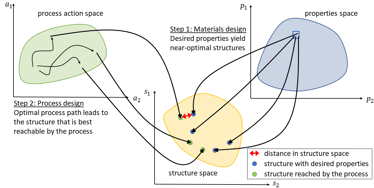
One fundamental characteristic of the process-structure-properties chain that can be leveraged is its modularity: Each individual link represents a specific identification problem, which includes identifying microstructures for given desired properties (materials design) and finding optimal processing paths for targeted microstructures (process design). These identification problems are typically not well-posed in the sense of Hadamard [5], which presents a significant challenge for solution approaches [6]. However, the non-unique nature of these problems offers an important advantage for processing: It enables a more flexible production as processes can be efficiently guided to manufacture the best reachable microstructure from a set of equivalent microstructures with respect to their properties.
The identification problems mentioned above remain highly complex and are often high-dimensional. To handle this complexity, the usage of machine learning has shown to be suitable for materials and process design applications[7, 8]. In this work, a novel machine learning framework is introduced that combines a reinforcement learning approach for multi-equivalent goal structure guided processing path optimization (MEG-SGGPO) [9] with a Siamese multi-task learning-based optimization (SMTLO) approach [10]. The framework is tailored to the specifics of process-structure-property optimization problems and therefore constitutes a significant advancement towards accelerated process and materials design.
Although each of the approaches have been shown to work well for their individual design problems, the combined usage of both is not investigated yet. This is particularly the aim of the present work, while the approach is enhanced by using a recently developed novel distance measure for one-point statistics microstructure representations: the Sinkhorn distance [11]. Specifically, the Sinkhorn distance is supposed to be suited well as it takes into account neighborhood information encoded in histogram-based microstructure representations. The importance of the distance measure can be seen in Figure 1, which depicts the general concept of the approach. In this work, we demonstrate the approach at manufacturing metallic materials with desired elastic and anisotropy properties, which are affected by the crystallographic texture that evolves during forming.
Pioneering work has already been done in this field, however, typically either focusing on solving materials design problems (without taking into account processing) or focusing on solving process design problems for given desired properties (not taking into account the structure of materials). In the following, we discuss works that describe approaches for solving materials and process design problems with an emphasize on the application of machine learning.
A widely-used approach for designing materials is the microstructure sensitive design (MSD) approach [12]. This approach primarily focuses on identifying microstructures that exhibit desired properties, with six out of the seven MSD steps being dedicated to this task. The processing of structures is only briefly addressed by the final MSD step. To the authors knowledge, there are only few works that show how to set up process-structure-property linkages for crystallographic texture optimization within the framework of MSD. One approach involves modeling texture evolution as fluid flow in the orientation space. On this basis, so-called processing streamlines are used to guide from one point to another [12, 13].
For example, in the case of optimizing the crystallographic texture of an orthotropic plate, these streamlines were calculated for the processing operations of tension and compression, and used to guide from a random texture to required textures [14]. These required textures have been identified in beforehand based on the MSD approach [15]. Alternatively, so-called texture evolution networks have been developed within the context of MSD, using a priory sampled processing paths to create a directed tree graph where microstructures are represented by the nodes on the graph [16]. Graph search algorithms are then used to find optimal processing paths from an initial to a targeted microstructures.
Besides the MSD approach, other approaches exist that solve crystallographic texture optimization problems in terms of materials design, however, without solving a corresponding optimal processing problem. For instance, Kuroda and Ikawa [17] used a genetic algorithm to identify optimal combinations of typical fcc rolling texture components for given desired properties. Also, Liu et al. [18] used optimization algorithms, but incorporated machine learning techniques to efficiently identify significant features and regions of the orientation space. Surrogate-based optimization has also been explored in several studies, such as for handling uncertainties in materials design [19]. Alternatively, probabilistic modeling approaches can be used to directly solve the inverse identification problem [20].
Regarding process design, machine learning-based and data mining-based approaches have been proposed by several works, however, without solving the corresponding materials design problem in beforehand. One approach involves the use of principle component analysis to represent one-step and two- to three-step deformation processes and to identify the deformation sequences required for reaching target crystallographic textures [21, 22]. Alternatively, a database approach can be used that stores microstructure representations and corresponding processing paths [23]. The database can be searched for desired textures yielding optimal process paths. These process paths can then be fine-tuned using gradient-based optimization. Another option is to store microstructure representations in a lower dimensional feature space generated by a variational autoencoder [24]. In this lower dimensional feature space, optimal processing paths can be identified using a suitable distance measure.
2 Results
In the following, we demonstrate how the machine learning approach can be used to identify process paths for manufacturing an optimal crystallographic texture for given desired properties in a metal forming process. The metal forming process used for this purpose consists of seven subsequent loading steps, each of 10% uniaxial strain. In each step, the uniaxial strain operation can be applied in one out of 25 different loading directions, leading to a constant change in crystallographic texture. Consequently, the there are different processing paths.
On this basis, in Section 2.1, it is shown how near-optimal crystallographic textures are identified for given elastic and anisotropy properties using the SMTLO approach. The properties are in particular the Young’s moduli and anisotropy measures , both in three orthogonal directions. Using the set of near-optimal crystallographic textures, in Section 2.2, it is shown how the MEG-SGGPO approach is used to guide the forming process to identify and manufacture the best reachable texture. Further details on the implementation of the machine learning models, the numerical simulation as well as the generation and representation of texture data can be found in Section 4.
2.1 Designing materials using SMTLO
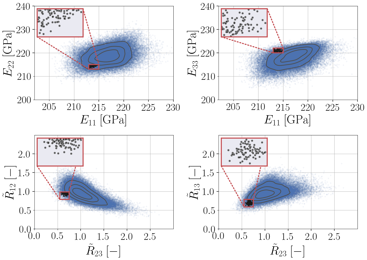
The basis for applying the SMTLO approach is a data set of 76980 samples, composed of textures and corresponding properties. 2D projections of the training data distribution, generated by the metal forming process simulation, are shown in Figure 2 including the region delineating the desired properties (target region). In this study, the target region is centered at GPa and . Its width equals GPa for and for . Both and are determined in three orthogonal directions at the material point at the end of the process. is given by the slope in the elastic regime, while is calculated by the ratio between transverse and tensile strain in the plastic regime when applying uniaxial tension. In Figure 2, we highlighted training data points that are already located inside the target region. We use this set of textures as benchmark set.
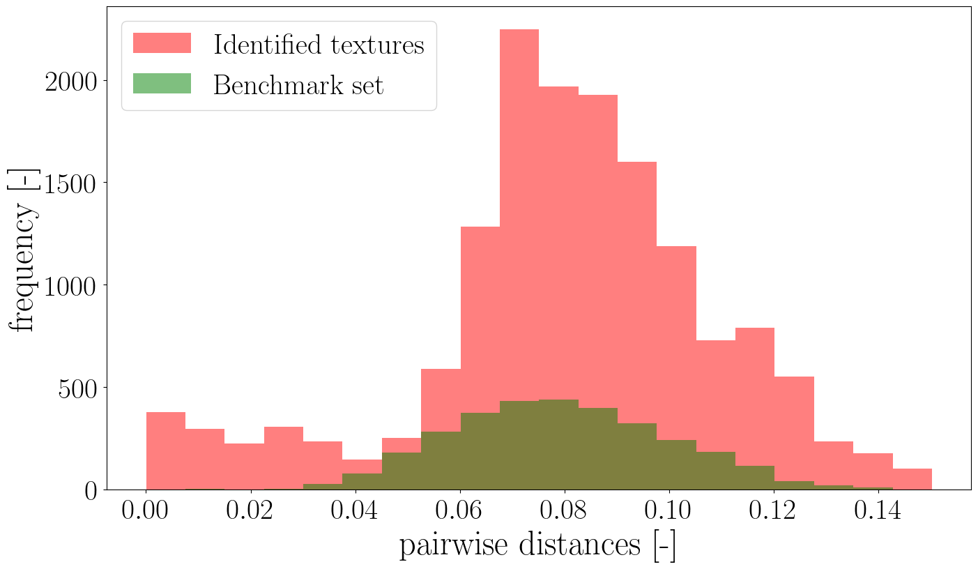
Using the SMTLO approach, we were able to identify a set of 175 near-optimal textures. As we aim to identify a preferably diverse set of textures, we depict their pairwise distances in Figure 3 and compare them to the benchmark set. As one can easily see, the SMTLO approach is able to find a set of textures that differ more to each other than the benchmark set.
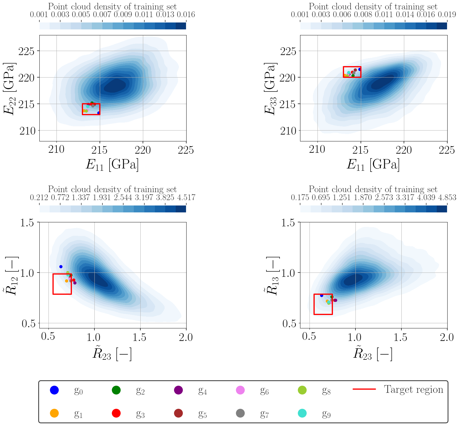
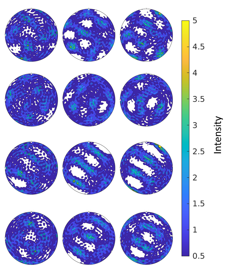
For the subsequent process design step, we chose ten goal textures from the set of identified textures that differ strongly from each other [25]. The distribution of the chosen goal textures in properties space is shown in Figure 4. The properties of the goal textures, however, are not located completely inside the target region. To show the differences between the goal textures, in Figure 5, four textures are depicted exemplary as pole figure plots. While the pole figure intensities are similar for all textures, the shape of the represented orientation distribution differs strongly.
2.2 Structure-guided process design using MEG-SGGPO
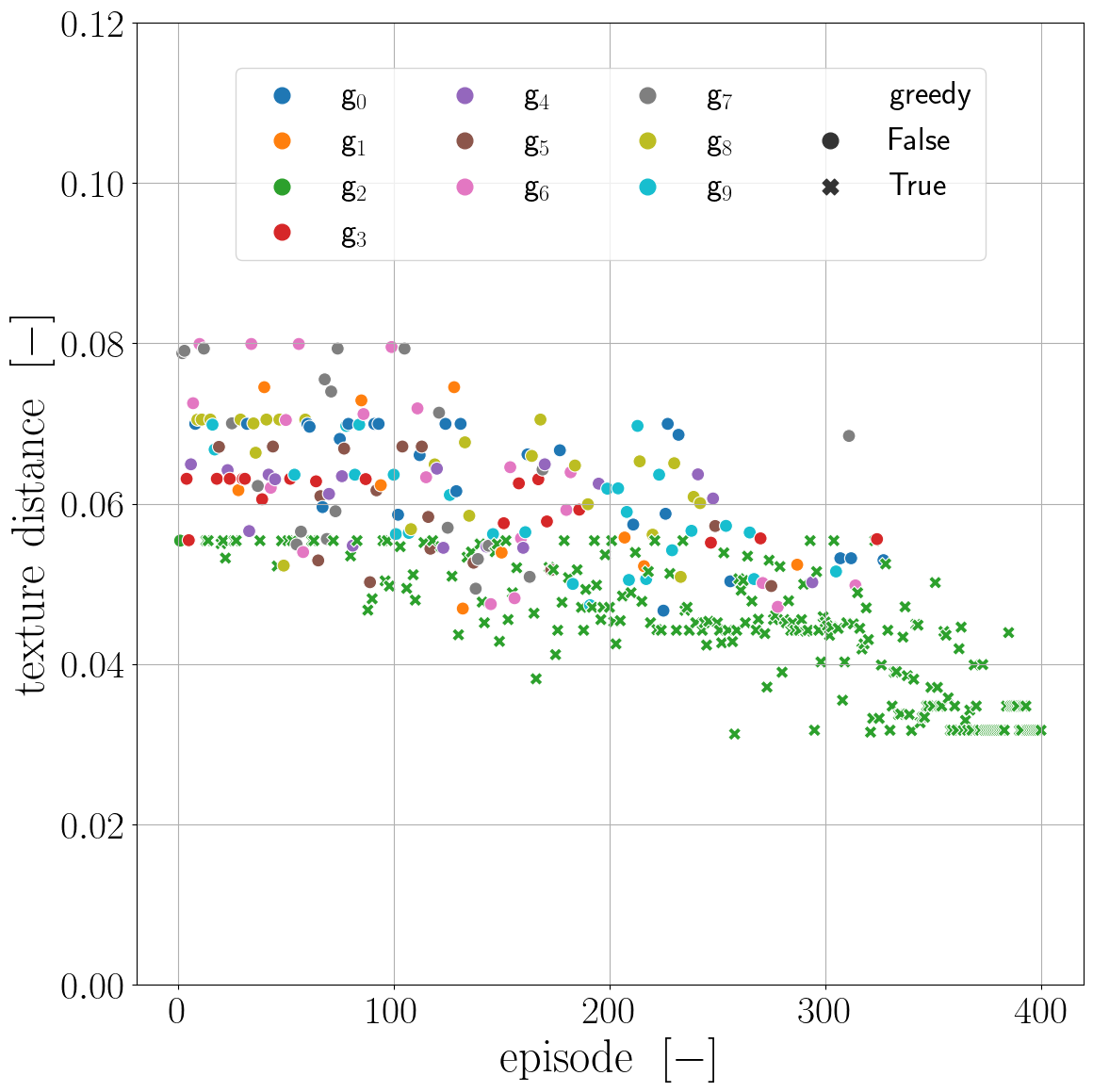
Once a diverse set of crystallographic textures has been identified, MEG-SGGPO is used to guide the metal forming process to the best reachable texture. For solving the identification problem, the MEG-SGGPO approach is allowed to conduct process runs, so-called episodes. The evolution of the distance between the produced and the chosen goal texture is depicted over the episodes in Fig. 6. Initially, the reinforcement learning agent attempts to identify processing paths that target randomly selected goal textures. As the learning process progresses, the agent focuses increasingly on producing goal texture .
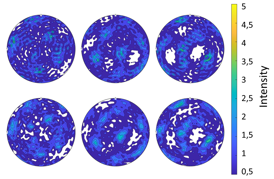
For comparison, Figure 7 presents pole figure plots of the goal texture and the produced texture after 400 episodes. Visually, the produced texture is highly similar to the goal texture with intensity peaks at the same positions and of a similar magnitude. This also holds for areas not covered by orientations at all. To quantify the effectiveness of the approach, we compute the properties resulting from the produced crystallographic texture and compare them with the desired ones. The results, listed in Table 1, show that five of the properties (, , , and ) are very close to the target region, while lies inside.
| Target property | Value | Distance to target region | Unit |
|---|---|---|---|
| 217.5 | 2.5 | GPa | |
| 216.6 | 1.6 | GPa | |
| 222.2 | 0.3 | GPa | |
| 0.744 | 0 | - | |
| 0.831 | 0.046 | - | |
| 1.058 | 0.073 | - |
In summary, by sequentially applying the SMTLO and the MEG-SGGPO approach, we were able to successfully produce a crystallographic texture with desired properties in a simulated metal forming process. The resulting properties fall within the acceptable range from an engineering point of view, albeit at the border of the defined properties region.
3 Discussion
The results presented in Section 2.1 demonstrate the effectiveness of the SMTLO approach in identifying sets of near-optimal crystallographic textures that exhibit desired properties in a given target region. The set of textures identified by the approach is shown to be more diverse than the benchmark set obtained from the training data set. However, the properties of the identified textures are not completely inside the target region, as can be seen in Fig. 4.
There are two reasons for this: First, the formulation of the optimization objective in the SMTLO approach allows for a trade-off between (i) finding crystallographic textures with properties inside the target region, (ii) identifying possibly diverse textures and, (iii) guaranteeing that texture can be produced by the process under consideration. Second, due to prediction errors of the underlying machine learning model, the SMTLO approach identifies textures whose predicted properties lie inside the target region, while the true properties (calculated by the numerical simulation) slightly lie outside. Both of these issues can be addressed by modifying the objective function. For instance, targeting the center of the properties region, instead of its bounds can mitigate both issues. Additionally, the second issue can be addressed by enhancing the machine learning model, for example, by increasing the amount of training data.
Taking a diverse subset of the identified textures as goal textures, the MEG-SGGPO approach guides the metal forming process closely to one of the chosen goal textures. Although the reinforcement learning agent was not able to reproduce one of the goal textures exactly (which is challenging due to the many possible processing paths), the measured distance between the targeted texture and the produced one is sufficiently low () when relating it to the distance to the nearest neighbor in the training data set () and to the furthest data point (). We want to remark here, that it took the reinforcement learning agent only 400 episodes to achieve this result compared to the baseline set that is grounded on the generation of 76980 random samples. The reinforcement learning algorithm can therefore be seen as being data efficient.
Nevertheless, in this study, it seems that a lower bound is existing that is difficult to overcome by the MEG-SSGPO approach. In general, this can have two reasons: First, the forming process is unable to produce textures that are closer to the goal texture identified by the SMTLO approach. Yet, the SMTLO approach already addresses this issue by enforcing microstructures to remain within the region delineated by the known microstructures from the training data set. We expected that a stronger enforcement leads to textures that are better reachable by the process. This, however, can lead to a less accurate properties prediction. Second, the MEG-SGGPO approach identified a local optimum and got stuck. This can be mitigated by longer MEG-SGGPO runs with optimized hyperparameters. Longer runs, however, have not shown to yield significant improvements in the presented study. As future work, it is desirable to incorporate the knowledge contained in the generated training samples for SMTLO into MEG-SGGPO a priori to enhance its performance.
On the whole, the machine learning-based approach presented in this study enables accelerated materials development while taking into account the manufacturing process. Particularly, we want to highlight that the considered metal forming process offers a total of different processing paths, and despite this complexity,
-
•
samples were sufficient for the SMTLO approach to successfully solve the materials design problem. It allowed us to identify a diverse set of near-optimal textures with desired properties.
-
•
a total of episodes was sufficient for the MEG-SGGPO approach to successfully guide the forming process successfully and solve the process design problem.
This shows that the applied approach is highly data efficient and capable of effectively optimizing process-structure-property relations end-to-end in manufacturing processes. Moreover, we want to emphasize that the approach leverages the non-uniqueness of the materials and process design problems, meaning that a diverse set of microstructures is identified for given desired properties and subsequently, the best reachable microstructure is produced. This is a significant advantage when transferring the approach to real manufacturing systems, where often constraints exist, which may exclude microstructures from being producible. Nonetheless, the application still needs to be validated in real manufacturing systems. In our specific case, the amount of used training data is comparably high to what is typically available in production. Thus, for application in manufacturing, a first step would be to pre-train the machine learning models with a numerical simulation that serves as a digital twin of the process and the material.
4 Methods
In this section, we present details about the approaches for materials and process design, SMTLO [10] and MEG-SGGPO [9], as well as the underlying metal forming simulation and the representation of crystallographic texture.
4.1 Metal forming process simulation
The metal forming process simulation [9] used in this study applies a deformation
| (1) |
with being a rotation matrix that describes one out of 25 possible loading directions. The deformation is defined using orthogonal basis vectors and the operator for the outer product
| (2) |
with corresponding to strain increments. are adjusted such that the stresses are in balance. The metal forming process consists of seven subsequent loading steps, each in a separate loading direction. For this study, we conducted 76980 random process paths to generate the training data for the SMTLO approach.
The underlying material model is a crystal plasticity model of Taylor-type [26]. The volume averaged stress for crystals with different orientations is calculated by
| (3) |
with the total volume , the individual volume of each crystal , and the Cauchy stress tensor .
With the multiplicative decomposition of the deformation gradient in its elastic and plastic part
| (4) |
and the conversion formula for the stress tensor in the intermediate configuration
| (5) |
the Cauchy stress tensor is derived using
| (6) |
where denotes the second order identity tensor and the fourth order elastic stiffness tensor.
The evolution of the plastic deformation is described using the plastic part of the velocity gradient
| (7) |
with the slip rates on slip system that is defined by the slip plane normal and the slip direction . The slip rates are calculated by a phenomenological power law. The crystal reorientation is calculated by applying a rigid body rotation derived from the polar decomposition of to the original orientation [27, 11].
4.2 Texture representation and distance measure
Texture is represented by using the histogram-based description introduced by Dornheim et al. [9]. The orientation histogram (soft-assignment factor of three) consists of 512 orientation bins that are nearly uniformly distributed in the cubic-triclinic fundamental zone, which were created using the software neper [28, 29]. In contrast to the original MEG-SGGPO approach, crystallographic texture distances are measured using the Sinkhorn distance applied to the histogramm representation [11]. Specifically, the Sinkhorn distance is an efficient implementation of the Earth Movers distance that measures the least amount of work necessary to transform one histogram into the other [30, 31]. Therefore, local orientation distances [32] encoded in the histograms are taken into account, in contrast to the originally proposed Chi-Squared distance, which is basically a bin-wise comparison of two histograms.
4.3 The SMTLO approach
The SMTLO approach described in [10] aims to identify diverse microstructures for given desired properties (defined by a target region). It consists of a multi-task learning model, which is grounded on an encoder that transforms a microstructure representation into a lower dimensional latent feature space representation
| (8) |
with the trainable parameters . The encoder is equipped with three heads, each of which is designed to solve a specific learning task. These are
-
1.
a decoder head that reconstructs the microstructure representations from
(9) with the trainable parameters . The encoder-decoder part is trained using a loss term that minimizes the Sinkhorn distance between the original microstructure and its reconstruction [11]
(10) -
2.
a prediction head to infer material properties
(11) with the trainable parameters . The sample-wise loss term is defined by the mean squared error between predicted and true properties
(12) with the number of properties .
-
3.
an auto-encoder head that serves as an anomaly detector to estimate whether a microstructure in its latent representation belongs to the set of known microstructures (defined by the training data) or not:
(13) with the encoder and decoder parts and and the trainable parameters and , respectively. The auto-encoder is trained using a mean squared error loss function
(14) with dimensions of the latent feature space.
A neural network is used to solve the above mentioned learning tasks, which is trained using a combined loss function
| (15) |
with individually weighted loss terms using the parameters , , and .
To ensure that the original microstructure distance is preserved in the latent feature space, a Siamese training method is applied [33]. This involves training two twin models simultaneously, with shared weights, and adding a further loss term that applies to the latent feature space. This preservation loss writes
| (16) |
with the absolute distance in the latent feature space
| (17) |
The superscripts (1) and (2) are used to distinguish between the two simultaneously trained twins parts. The overall loss function writes
| (18) |
with the regularization term , , and .
In order to identify microstructures with desired properties, we use a genetic optimizer [34] to search for candidate microstructures in the latent feature space generated by the Siamese multi-task learning model. The optimizer minimizes three cost terms: [10]. minimizes the distance of the predicted property for a candidate microstructure to the target region. penalizes candidate microstructures that are not inside the region of known microstructures. enforces candidate microstructures being as far away as possible from each other in the actual population. The overall objective function writes
| (19) |
with individual weights , , and .
4.4 The MEG-SGGPO approach
In reinforcement learning, an agent learns to take optimal decisions by interacting with its environment in a sequence of discrete time steps . The MEG-SGGPO approach [9] is tailored for efficient learning in the case of multiple equivalent target microstructures. Given a set of near-optimal microstructures , an initial microstructure , and a microstructure generating process , the goal of the approach is to find a sequence of processing parameters that guide the process towards manufacturing the best reachable microstructure .
MEG-SGGPO is based on deep Q-networks[35] and its extensions [36, 37, 38]. Deep Q-networks are derived from Q-learning, where the so-called Q-function is approximated from data gathered by the reinforcement learning agent while following a policy . The Q-function models the expected sum of future reward signals for state action pairs . In MEG-SGGPO the Q-function is generalized to also take the goal microstructure into account and is, in its recursive form, defined as
| (20) |
where is a per goal microstructure pseudo reward function
| (21) |
which is based on a microstructure distance function .
The process design task is a two-fold optimization problem to(i) identify the best reachable goal microstructure and (ii) learn the optimal policy . MEG-SGGPO addresses this by using the generalized functions defined above in a nested reinforcement learning procedure. At the beginning of each episode (i.e. an execution of the process during learning), the agent uses the generalized Q-function to identify the targeted microstructure from and determines the processing parameters during the episode. In a first step, an estimation of the best reachable goal microstructure is extracted from the current estimation by
| (22) |
where the generalized state-value function is defined as
| (23) |
The targeted microstructure is chosen in an -greedy approach [39], where the agent chooses random targets and processing parameters in an fraction of the cases () and optimizes targets and processing parameters in the remaining cases. The optimal processing path is identified simultaneously in an inner loop by using the Q-learning approach.
Data availability statement
Data and code has been published in the following repositories:
-
•
Training data for the SMTLO approach is made available via Fraunhofer Fordatis repository at https://fordatis.fraunhofer.de/handle/fordatis/319 [40].
-
•
The process simulation is made available via Fraunhofer Fordatis repository at https://fordatis.fraunhofer.de/handle/fordatis/201.2[41].
-
•
The source code for the Siamese multi-task learning framework is made available via gitlab at https://gitlab.com/tarekiraki/the_smtl_framework.
-
•
The reinforcement learning environment is made available via github at https://github.com/Intelligent-Systems-Research-Group/RL4MicrostructureEvolution.
Acknowledgments
The authors would like to thank the German Research Foundation (DFG) for funding this work, which was carried out within the research project number 415804944: ’Taylored Material Properties via Microstructure Optimization: Machine Learning for Modelling and Inversion of Structure-Property-Relationships and the Application to Sheet Metals’.
Author contribution
LM set up the numerical simulation, generated the training data for solving the materials design problem and wrote the manuscript together with all other authors. TI developed the SMTLO approach and applied both, the SMTLO and the MEG-SGGPO approach to the problem analyzed in this study. JD developed the MEG-SGGPO approach. The approach was extended using the Sinkhorn distance measure by TI. SS supported in terms of machine learning and materials science. NL supported in terms of machine learning. DH supported in terms of materials science. All authors contributed equally to the discussion of the results and to reviewing the manuscript.
Competing interests
The authors have no competing interests to declare that are relevant to the content of this article.
References
- [1] J. J. de Pablo, N. E. Jackson, M. A. Webb, L.-Q. Chen, J. E. Moore, D. Morgan, R. Jacobs, T. Pollock, D. G. Schlom, E. S. Toberer, et al., “New frontiers for the materials genome initiative,” npj Computational Materials, vol. 5, no. 1, p. 41, 2019.
- [2] Advanced materials initiative 2030, “The materials roadmap 2030,” tech. rep., 2022.
- [3] P. Grant, “Foresight – new and advanced materials,” tech. rep., 2013.
- [4] G. B. Olson, “Computational design of hierarchically structured materials,” Science, vol. 277, no. 5330, pp. 1237–1242, 1997.
- [5] J. Hadamard, “Sur les problèmes aux dérivées partielles et leur signification physique,” Princeton university bulletin, pp. 49–52, 1902.
- [6] A. Agrawal and A. Choudhary, “Perspective: Materials informatics and big data: Realization of the “fourth paradigm” of science in materials science,” Apl Materials, vol. 4, no. 5, p. 053208, 2016.
- [7] Y. Liu, T. Zhao, W. Ju, and S. Shi, “Materials discovery and design using machine learning,” Journal of Materiomics, vol. 3, no. 3, pp. 159–177, 2017.
- [8] M. Mozaffar, S. Liao, X. Xie, S. Saha, C. Park, J. Cao, W. K. Liu, and Z. Gan, “Mechanistic artificial intelligence (mechanistic-ai) for modeling, design, and control of advanced manufacturing processes: Current state and perspectives,” Journal of Materials Processing Technology, vol. 302, p. 117485, 2022.
- [9] J. Dornheim, L. Morand, S. Zeitvogel, T. Iraki, N. Link, and D. Helm, “Deep reinforcement learning methods for structure-guided processing path optimization,” Journal of Intelligent Manufacturing, vol. 33, pp. 333–352, 2021.
- [10] T. Iraki, L. Morand, J. Dornheim, N. Link, and D. Helm, “A multi-task learning-based optimization approach for finding diverse sets of material microstructures with desired properties and its application to texture optimization,” Journal of Intelligent Manufacturing, 2023.
- [11] T. Iraki, L. Morand, N. Link, S. Sandfeld, and H. Dirk, “Accurate distances measures and machine learning of the texture-property relation for crystallographic textures represented by one-point statistics,” arXiv:2312.04214, 2023.
- [12] D. T. Fullwood, S. R. Niezgoda, B. L. Adams, and S. R. Kalidindi, “Microstructure sensitive design for performance optimization,” Progress in Materials Science, vol. 55, no. 6, pp. 477–562, 2010.
- [13] D. Li, H. Garmestani, and S. Ahzi, “Processing path optimization to achieve desired texture in polycrystalline materials,” Acta materialia, vol. 55, no. 2, pp. 647–654, 2007.
- [14] B. L. Adams, S. Kalidindi, D. T. Fullwood, and D. Fullwood, Microstructure sensitive design for performance optimization. Butterworth-Heinemann, 2012.
- [15] S. R. Kalidindi, J. R. Houskamp, M. Lyons, and B. L. Adams, “Microstructure sensitive design of an orthotropic plate subjected to tensile load,” International Journal of Plasticity, vol. 20, no. 8-9, pp. 1561–1575, 2004.
- [16] J. B. Shaffer, M. Knezevic, and S. R. Kalidindi, “Building texture evolution networks for deformation processing of polycrystalline fcc metals using spectral approaches: Applications to design for targeted performance,” International Journal of Plasticity, vol. 26, no. 8, pp. 1183–1194, 2010.
- [17] M. Kuroda and S. Ikawa, “Texture optimization of rolled aluminum alloy sheets using a genetic algorithm,” Materials Science and Engineering: A, vol. 385, no. 1-2, pp. 235–244, 2004.
- [18] R. Liu, A. Kumar, Z. Chen, A. Agrawal, V. Sundararaghavan, and A. Choudhary, “A predictive machine learning approach for microstructure optimization and materials design,” Scientific Reports, vol. 5, no. 1, pp. 1–12, 2015.
- [19] P. V. Balachandran, D. Xue, J. Theiler, J. Hogden, and T. Lookman, “Adaptive strategies for materials design using uncertainties,” Scientific reports, vol. 6, no. 1, pp. 1–9, 2016.
- [20] A. Tran and T. Wildey, “Solving stochastic inverse problems for property–structure linkages using data-consistent inversion and machine learning,” JOM, vol. 73, no. 1, pp. 72–89, 2021.
- [21] P. Acar and V. Sundararaghavan, “Linear solution scheme for microstructure design with process constraints,” AIAA Journal, vol. 54, no. 12, pp. 4022–4031, 2016.
- [22] P. Acar and V. Sundararaghavan, “Reduced-order modeling approach for materials design with a sequence of processes,” AIAA Journal, vol. 56, no. 12, pp. 5041–5044, 2018.
- [23] V. Sundararaghavan and N. Zabaras, “On the synergy between texture classification and deformation process sequence selection for the control of texture-dependent properties,” Acta materialia, vol. 53, no. 4, pp. 1015–1027, 2005.
- [24] S. Sundar and V. Sundararaghavan, “Database development and exploration of process–microstructure relationships using variational autoencoders,” Materials Today Communications, vol. 25, p. 101201, 2020.
- [25] C. Bauckhage, “Ml2r coding nuggets: Hopfield nets for max-sum diversification,” 2021.
- [26] S. R. Kalidindi, C. A. Bronkhorst, and L. Anand, “Crystallographic texture evolution in bulk deformation processing of fcc metals,” Journal of the Mechanics and Physics of Solids, vol. 40, no. 3, pp. 537–569, 1992.
- [27] X. Ling, M. Horstemeyer, and G. Potirniche, “On the numerical implementation of 3d rate-dependent single crystal plasticity formulations,” International Journal for Numerical Methods in Engineering, vol. 63, no. 4, pp. 548–568, 2005.
- [28] R. Quey, P. Dawson, and F. Barbe, “Large-scale 3d random polycrystals for the finite element method: Generation, meshing and remeshing,” Computer Methods in Applied Mechanics and Engineering, vol. 200, no. 17-20, pp. 1729–1745, 2011.
- [29] R. Quey, A. Villani, and C. Maurice, “Nearly uniform sampling of crystal orientations,” Journal of Applied Crystallography, vol. 51, no. 4, pp. 1162–1173, 2018.
- [30] Y. Rubner, C. Tomasi, and L. J. Guibas, “The earth mover’s distance as a metric for image retrieval,” International Journal of Computer Vision, vol. 40, pp. 99–121, 2000.
- [31] M. Cuturi, “Sinkhorn distances: Lightspeed computation of optimal transport,” in Advances in Neural Information Processing Systems (C. J. C. Burges, L. Bottou, M. Welling, Z. Ghahramani, and K. Q. Weinberger, eds.), vol. 26, Curran Associates, Inc., 2013.
- [32] D. Q. Huynh, “Metrics for 3D rotations: Comparison and analysis,” Journal of Mathematical Imaging and Vision, vol. 35, no. 2, pp. 155–164, 2009.
- [33] J. Bromley, I. Guyon, Y. LeCun, E. Säckinger, and R. Shah, “Signature verification using a” siamese” time delay neural network,” Advances in neural information processing systems, vol. 6, 1993.
- [34] J. Zhang and A. C. Sanderson, “Jade: Adaptive differential evolution with optional external archive,” IEEE Transactions on Evolutionary Computation, vol. 13, no. 5, pp. 945–958, 2009.
- [35] V. Mnih, K. Kavukcuoglu, D. Silver, A. A. Rusu, J. Veness, M. G. Bellemare, A. Graves, M. Riedmiller, A. K. Fidjeland, G. Ostrovski, et al., “Human-level control through deep reinforcement learning,” nature, vol. 518, no. 7540, pp. 529–533, 2015.
- [36] H. Van Hasselt, A. Guez, and D. Silver, “Deep reinforcement learning with double q-learning,” in Thirtieth AAAI conference on artificial intelligence, 2016.
- [37] T. Schaul, J. Quan, I. Antonoglou, and D. Silver, “Prioritized experience replay,” arXiv:1511.05952, 2015.
- [38] Z. Wang, T. Schaul, M. Hessel, H. Van Hasselt, M. Lanctot, and N. De Freitas, “Dueling network architectures for deep reinforcement learning,” arXiv:1511.06581, 2015.
- [39] R. S. Sutton, A. G. Barto, and R. J. Williams, “Reinforcement learning is direct adaptive optimal control,” IEEE control systems magazine, vol. 12, no. 2, pp. 19–22, 1992.
- [40] L. Morand, T. Iraki, and D. Helm, “Crystallographic texture-property data set originating from a simulated multi-step metal forming process,” 2023. - Fraunhofer Fordatis repository https://fordatis.fraunhofer.de/handle/fordatis/319.
- [41] L. Morand, J. Dornheim, J. Pagenkopf, and D. Helm, “Simulation of texture evolution for a multi-step metal forming process,” 2021. - Fraunhofer Fordatis repository https://fordatis.fraunhofer.de/handle/fordatis/201.2.