A machine learning approach based on survival analysis for IBNR frequencies in non-life reserving

Abstract

We introduce new approaches for forecasting IBNR (Incurred But Not Reported) frequencies by leveraging individual claims data, which includes accident date, reporting delay, and possibly additional features for every reported claim. A key element of our proposal involves computing development factors, which may be influenced by both the accident date and other features. These development factors serve as the basis for predictions. While we assume close to continuous observations of accident date and reporting delay, the development factors can be expressed at any level of granularity, such as months, quarters, or year and predictions across different granularity levels exhibit coherence. The calculation of development factors relies on the estimation of a hazard function in reverse development time, and we present three distinct methods for estimating this function: the Cox proportional hazard model, a feed-forward neural network, and xgboost (eXtreme gradient boosting). In all three cases, estimation is based on the same partial likelihood that accommodates left truncation and ties in the data. While the first case is a semi-parametric model that assumes in parts a log linear structure, the two machine learning approaches only assume that the baseline and the other factors are multiplicatively separable. Through an extensive simulation study and real-world data application, our approach demonstrates promising results. This paper comes with an accompanying R-package, ReSurv, which can be accessed at https://github.com/edhofman/ReSurv.

1 Introduction

IBNR (Incurred But Not Reported) refers to outstanding claims for which the insurer is liable but which have not been reported at the time the reserve is calculated. Empirical studies on insurance markets show that in many lines of business the estimated cost of IBNR claims is the most important provision for the insurer, see for example (Friedland, 2010, p. 80). As the number of IBNR claims is not known at the time the reserve is calculated, there is a strong actuarial argument in favour of methods that accurately predict the number of IBNR claims.

In the seminal paper miranda2013continuous, the authors discuss how the common run-off triangles encountered in loss reserving in non-life insurance can be understood within a continuous framework where the goal is to estimate the distribution in the lower triangle. Within this continuous chain-ladder framework, two lines of research emerged: One aims to estimate the underlying density function and with this respect, lee15, lee17, and mammen21 generalize the initial model to account for seasonal effects, operation al time and calendar effects, respectively. In the other line of research, Hiabu . (2016) establishes that the observation scheme of a continuous run-off triangle can be understood as right-truncation problem and that by reversing the development time statistical analysis can be conducted under a tractable left-truncation setting. Building on this work, Hiabu (2017) discusses how the hazard function in reverse development time is related to the omnipresent development factors. Hiabu . (2021) extends the framework by allowing for accident date effects and other features via a multiplicative structure. Bischofberger . (2020) extends the prediction of claim frequencies to the prediction of claim payments. A simulation study comparing the two lines of research can be found in Bischofberger . (2019).

A major drawback of both lines of research so far is that they have not been very practical: Estimation is based on kernel smoothers that without further adjustment do not cope well with the sharp patterns often seen in claim developments. Additionally, it is not directly clear how to include categorical features. In fact, with the exception of Hiabu . (2021) that allows for continuous features, none of the other work so far considers additional features, neither continuous nor categorical. A limiting factor is that if no structure is imposed a priori, kernel smoother will necessarily suffer from the curse of dimensionality, i.e., exponentially deteriorating estimation performance with every continuous feature added. Machine learning methods on the other hand have shown that they are capable of data-driven dimension reduction and making use of the underlying data structure in order to circumvent the curse of dimensionality. With these considerations, and within the second line of research, we propose three methods to estimate an accident date and other features dependent hazard function: the Cox proportional hazard model, a feed-forward neural network and xgboost.

In all of the three proposed methods, estimation will be based on the same partial likelihood that accommodates left truncation and ties in the data. While there is a growing number of survival analysis solutions being implemented for common machine learning methods, to the best of our knowledge, neither of the publicly available feed-forward neural network solution nor xgboost solutions have implementations that can deal with left-truncated data and ties in the data Wiegrebe . (2023). Hence, to make our proposal work, we will extend current xgboost and feed-forward neural networks solutions such that they can handle left truncation and ties under the assumption that ties correspond to intervals in which events happen uniformly.

As mentioned before, we will use the estimated hazard function to calculate development factors which we will subsequently use for prediction. With this respect, our proposal is related to the approach of Wüthrich (2018) that uses a feed-forward neural network to estimate the development factors directly. One major advantage of our survival analysis approach is that we do not have problems with zero entries in the cumulative run-off triangles. In Wüthrich (2018), the loss function fed into the neural network entails dividing by each cumulative entry, see equation (3.1) in that paper. While zero entries are not common in typical run-off triangles, zero entries are expected to happen often if the features take too many different values resulting in many sparse triangles. In particular, the approach of Wüthrich (2018) does not allow for continuous features. To circumvent the problem of some zero entries with discrete or categorical features, Wüthrich (2018) proposes some adhoc method that ignores features in those entries. In contrast to that, in our approach we do not have those problems with zero entries and are able to estimate a conditional hazard function which is possibly dependent on high dimensional feature information.

In a recent preprint, Calcetero-Vanegas . (2023) aim to estimate the same hazard function as we propose to estimate. However, they only apply the Cox-proportional hazard model and not further machine learning methods as we do. Furthermore, they use an inverse probability weighting for prediction. In contrast, we propose to transform the hazard function into development factors which are subsequently used for prediction. While both approaches will produce similar predictions, one advantage of our proposal is the ease of comparison with standard reserving methods based on development factors; see the next section.

We organize our manuscript as follows. We conclude the introduction of this manuscript in Section 1.1, where we show an overview of the models development factors output based on xgboost on a simulated dataset. In Section 2 we introduce the continuous time framework and the hazard function we wish to estimate, while Section 3 introduces various estimation strategies. Section 4 establishes the connection between the estimated hazard functions and development factors. In Section 5 we discuss the performance measures that we will use in the empirical analyses to select and compare our models. In Section 6 we will challenge our models on several data sets simulated from $5$ different scenarios. In Section 7 we present an application on a real dataset from a Danish insurer. The dataset is not publicly available. We conclude the manuscript with general remarks on our approach.

1.1 Overview of the main model output

In recent years, there has been a growing number of papers developing reserving methods based on individual data; also known as micro-level reserving or granular reserving. See e.g. Lopez  Milhaud (2021); Fung . (2022); Crevecoeur . (2022) for some recent contributions and references therein.

The complexity of micro-level models make their practical implementation demanding. In particular, these models often demand some kind of calibration which can substantially influence the resulting outputs. Complicating matters further, it’s challenging to compare their fitting with established methods like the Chain-Ladder technique. Consequently, despite the potential for more accurate estimations, many actuarial practitioners remain hesitant to adopt them.

In this brief excerpt we aim to show how our model output can be visualized in a way familiar to reserving actuaries. It also allows a seamless comparison with estimations obtained through the chain ladder approach. To this end, we show a preview of the results that we obtained on a simulated data set coming from scenario Delta, as will be introduced in Section 6. In our simulation study, a claim can be of claim_type 0 or claim_type 1. In scenario Delta, we consider a seasonality effect in the accident date dimension which is different for claim_type 0 and claim_type 1. This could occur in a real world setting with an increased work load during winter for certain claim types, or a decreased workforce during the summer holidays. An important feature of our proposal is that while inputs are assumed continuous, development factors and predictions can be provided on chosen granularity levels. Oppositely to the chain ladder model the predicted development factors will depend on accident date and additional feature information; here claim type being equal zero or one. In Figure 1 we select one simulation and compare the chain ladder development factors to our output development factors for different granularities (monthly and yearly). The first row shows chain ladder’s development factors. The second row shows the output on a monthly level from an xgboost fit for three different feature combinations of accident date and claim type. The three plots can be compared to the monthly development factors obtained from chain ladder (first row left panel). The third row is the analogue to the second row, but this time a yearly aggregation has been chosen and it can be compared to the yearly development factors obtained from chain ladder (first row right panel).

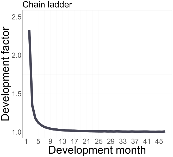
(a)

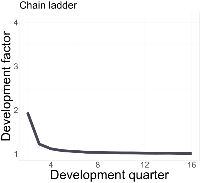
(b)

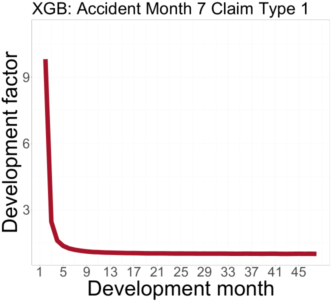
(c)

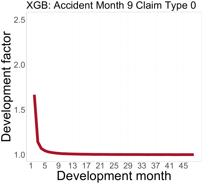
(d)

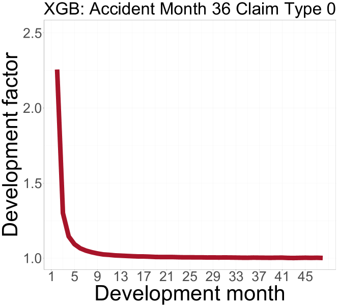
(e)

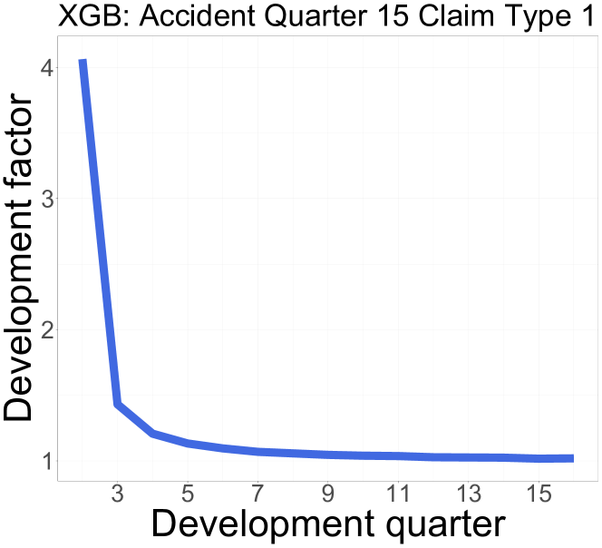
(f)

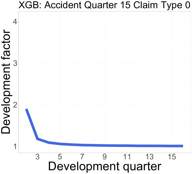
(g)

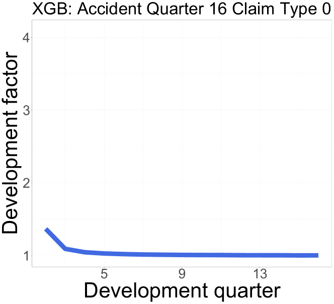
(h)

Figure 1: The first row, shows the chain ladder development factors fitted on monthly data (1(a)), and quarterly data (1(b)). The development factors do not consider additional features we have at our disposal. The second and third row show an xgboost output from our model proposal that depends on accident date and claim type. The second row, shows monthly development factors for the feature combinations Accident Month 7 and Claim_type 1 (left panel), Accident Month 9 and Claim_type 0 (center panel) and Accident Month 36 and Claim_type 1 (right panel). The third row shows quarterly development factors for the feature combinations Accident Quarter 15 and Claim_type 1 (left panel), Accident Quarter 15 and Claim_type 0 (center panel) and Accident Quarter 16 and Claim_type 0 (right panel).

2 Modeling

At a cut-off-date $\mathcal{T}$, we have observed $n$ claim reports. For each claim $i$ with $i=1,\dots,n$, we are given the accident date $U_{i}$ and the time delay from accident until report, $T_{i}$. Suppose that for each individual we have at our disposal a set of $p$ measurements, i.e. the features ${X}_{i}\in\mathbb{R}^{p}$. We assume that

1. All reportings are independent.

Assumptions [A1] is made to simplify the mathematical derivations and we conjecture that it can be relaxed by considering weak dependency between reportings. Direct inference on $T_{i}$ may lead to sampling bias, as $T_{i}$ are observed only if the report happens before the cut-off date $\mathcal{T}$:

$$T_{i}\leq\mathcal{T}-U_{i},$$

which is a right-truncation problem. A solution to the right-truncation problem is to reverse the time of the counting process leading to a tractable left-truncation problem Ware  DeMets (1976). Concretely, we target $\mathcal{T}-T_{i}$ instead of $T_{i}$ such that the right truncation problem is now a left truncation problem ($\mathcal{T}-T_{i}\geq U_{i}$) with truncation variable $U_{i}$. We consider the development-time reversed counting processes

$$N_{i}(t)=I(t\geq\mathcal{T}-T_{i}),$$

each with respect to the filtration $\mathcal{F}_{it}=\sigma\left(\bigg{\{}T_{i}-\mathcal{T}\leq s:\ s\leq t\bigg{\}}\cup\bigg{\{}U_{i}\leq s:s\leq t\bigg{\}}\cup\bigg{\{}X_{i}\bigg{\}}\cup\mathcal{N}\right)$, satisfying the usual conditions (Andersen ., 2012, p. 60), and where $\mathcal{N}$ is the set of all zero probability events. In this paper, we will assume that $U_{i}$ and $T_{i}$ are encoded such that $0\leq U_{i}\leq\mathcal{T};0\leq T_{i}\leq\mathcal{T}$ and we are interested in predictions within the set $\{(t,u):(t,u)\in[0,\mathcal{T}]^{2}\}$.

2.1 The intensity process

Assuming that the intensity $\lambda_{i}$ of the counting process exists and is piecewise continuous, we have

$$\lambda_{i}(\mathcal{T}-t|U_{i},{X}_{i})=\lim_{h\downarrow 0}h^{-1}E\left[N_{i}\left\{(\mathcal{T}-t+h)-\right\}-N_{i}(\mathcal{T}-t)-|\ \mathcal{F}_{i,(\mathcal{T}-t)-}\right]=\alpha(t|U_{i},{X}_{i})Y_{i}(t),$$ (1)

where

$$\alpha(t|{u},{x}) =\lim_{h\downarrow 0}h^{-1}{P}\left(T_{i}\in(t-h,t]|\ Y_{i}(t)=1,{X_{i}}={x}_{i},U_{i}=u\right),$$

$$Y_{i}(t) =I(T_{i}\leq t<\mathcal{T}-U_{i}).$$

Note that $Y_{i}(t)$ and $\alpha(t|U_{i},X_{i})$ correspond to the intensity $\lambda_{i}(\mathcal{T}-t|U_{i},{X}_{i})$, meaning the development time input for $Y_{i}(t)$ and $\alpha(t|U_{i},X_{i})$ is not in reversed direction. The structure, $\lambda_{i}(\mathcal{T}-t|U_{i},{X}_{i})=\alpha(t|U_{i},{X}_{i})Y_{i}(t)$, is called Aalen’s multiplicative intensity model Aalen (1978), and enables nonparametric estimation and inference on the deterministic hazard function $\alpha(t|u,x)$. We propose to model the hazard function as

$$\alpha(t|u,x)=\alpha_{0}(t)e^{\phi\left(x,u;\theta\right)},$$ (2)

where $\alpha_{0}(t)$ is called the baseline hazard and $e^{\phi\left(x,u;\theta\right)}$ is the risk score; a component that depends on the features ${X}_{i}$ and the accident period $U_{i}$ and some parameters $\theta$. Assuming that the effects of $t$ and $u$ are multiplicatively separated allows us to have predictions for $\alpha$ in the lower triangle, $t>\mathcal{T}-u$, without extrapolation. In the next sections, we will discuss how to specify and model the log-risk function $\phi\left(x,u;\theta\right)$. We will consider three different models: the cox model <COX,>cox72, neural networks <NN,>katzman18 and gradient boosting <XGB,>friedman01,chen16.

• In cox72, the log-risk function is assumed to be linear, $\phi\left(x,u;\theta\right)=\theta^{T}x+\theta_{u}u$, with $\theta\in\mathbb{R}^{p}$ and $\theta_{u}\in\mathbb{R}$. In this paper we will consider the more general log-risk function that includes splines for modeling continuous features.

• In NN, the parameter $\theta$ represents the weights of a feed-forward neural network.

• In XGB, the log-risk function is an ensemble of decision trees, i.e., functions piecewise constant on rectangles.

3 Estimation

3.1 Ties in the data

Some reporting delays $T_{i}$ of different claims could be recorded with the same value, especially when the data records are not very granular. For example data with yearly, quarterly or even daily records will most certainly have multiple occurrences at the same reporting period. In survival analysis, the occurrence of multiple events at a given time point is known as a tie. In this section, we will adopt a general formulation of the problem to account for the incidental presence of ties in the data. We assume that for $i=1,\ldots,n$, reporting times $T_{i}$ are one of

$$t^{\left(0\right)}<\ldots<t^{\left(m\right)}<\ldots<t^{(M)},$$

with $M\leq n$. The rank of the observations within the tie does not affect the calculations that we will explain in this section. For notational convenience, we assume that observations are ordered from lowest to highest reporting time: $T_{i}\leq T_{j}$ for $i<j$. For $m=1,\ldots,M$, let us define, at the generic time $t^{(m)}$, the exposure set

$$\mathcal{R}(t^{(m)})=\{i\in\left\{1,\ldots,n\right\}:Y_{i}(t^{(m)})=1\}=\left\{i\in\left\{1,\ldots,n\right\}:T_{i}\leq t^{(m)};\ \mathcal{T}-U_{i}>t^{(m)}\right\}$$

and the occurrence set

$$\mathcal{O}(t^{(m)})=\left\{i\in\left\{1,\ldots,n\right\}:T_{i}=t^{(m)}\right\},$$

while we indicate with $O_{m}=\#\mathcal{O}(t^{(m)})$ the cardinality of the set $\mathcal{O}(t^{(m)})$.

To obtain an estimate of $\theta$, we will first formulate the partial likelihood in a general form and then we will specify the log-risk function. The specifications we use (COX, NN, XGB) were briefly introduced in Section 2.1 and they are the main focus of the current section. While the current literature on machine learning for survival analysis is about defining a model for right-censored data Chen  Guestrin (2016); Katzman . (2018), we contribute by extending the neural network in katzman18 and the gradient boosting machine in chen16 to define a framework for modeling left-truncated data with ties.

3.2 Partial likelihood

There are several approaches to account for the presence of ties in the data, see for instance [p. 85]hosmer08. We use the partial likelihood correction for ties presented in [Section 6, point g]efron77

$$\mathcal{L}({X}_{1},\ldots,{X}_{n};U_{1},\ldots,U_{n};\theta)=\prod_{m=1}^{M}\prod_{i\in\mathcal{O}(t^{(m)})}\frac{e^{\phi\left({X}_{i},{U}_{i};\theta\right)}}{\sum_{k\in\mathcal{R}(t^{(m)})}e^{\phi\left({X}_{k},U_{k};\theta\right)}-\frac{\psi_{i}(m)}{{O_{m}}}\sum_{s\in\mathcal{O}(t^{(m)})}e^{\phi\left({X}_{s},U_{s};\theta\right)}}$$

where $\psi_{i}(m)=i-\sum^{m-1}_{q=1}O_{q}-1$. Note that $\psi_{i}(m)\in\{0,\dots O_{m}-1\}$. To ease the notation, let us denote the partial likelihood as $\mathcal{L}(\theta)$. The negative log-likelihood is

$$l(\theta)=-\log(\mathcal{L}(\theta))=\sum_{m=1}^{M}\sum_{i\in\mathcal{O}(t^{(m)})}\log\left(\sum_{k\in\mathcal{R}(t^{(m)})}e^{\phi\left({X}_{k},U_{k};\theta\right)}-\frac{\psi_{i}(m)}{O_{m}}\sum_{s\in\mathcal{O}(t^{(m)})}e^{\phi\left({X}_{s},U_{s};\theta\right)}\right)-\phi\left({X}_{i},{U}_{i};\theta\right).$$ (3)

3.2.1 Cox model (COX)

The Cox proportional model uses a linear function to specify $\phi\left(X,U;\theta\right)=\theta^{T}X+\theta_{u}U$, with $\theta\in\mathbb{R}^{p}$ and $\theta_{u}\in\mathbb{R}$. To model continuous features that avoid the linear scale, we follow the approach in gray92 and introduce splines in the log-risk function Eilers  Marx (1996). Assuming that within the $p$ features we have $c$ features for the linear term $(X_{1},\ldots,X_{c})$ and $p-c$ features for the splines $(X_{c+1},\ldots,X_{p})$, the log-risk function is

$$\phi\left(X,U;\theta\right)=\sum^{c}_{l=1}\theta_{l}X_{l}+\sum^{p}_{s=c+1}\zeta_{s}\left(X_{s}\right)+\zeta_{u}\left(U\right),$$

where, for $V=U$ or $X_{l}$, $\zeta_{v}\left(V\right)=\sum_{k=0}^{\kappa_{v}}\beta^{v}_{k}B_{k}(V)$ and $\mathbf{\beta}^{v}=\left(\beta^{v}_{1},\ldots,\beta^{v}_{\kappa_{v}}\right)\in\mathbb{R}^{\kappa_{v}}$. Here, $B^{v}_{k}(V)$ are basis functions and $\kappa_{v}\in\mathbb{N}$ is the number of knots in the spline. The smoothing of $U$ and the other $p-c$ features modeled with splines are controlled with an additional penalty term in the log-partial likelihood during the model fitting. In the fitting phase we minimize the penalized likelihood

$$l^{p}(\theta,\beta^{c+1},\ldots,\beta^{p},\beta^{u})=l(\theta)-\frac{1}{2}\sum_{s}\rho_{s}\int\left[\zeta_{s}^{\prime\prime}(z)\right]^{2}dz-\frac{1}{2}\rho_{u}\int\left[\zeta_{u}^{\prime\prime}(z)\right]^{2}dz$$

with $\rho_{c+1},\ldots,\rho_{p},\rho_{u}$ being the parameter controlling the smoothing applied (no penalty for $\rho=0$ and forcing the spline to a linear form for $\rho=+\infty$). Noting that $\int\left[\zeta_{s}^{\prime\prime}(z)\right]^{2}dz$ is a quadratic form of $\mathbf{\beta}^{s}$, for some definite positive matrix $\mathbf{P}_{s}$, the penalized likelihood can be rewritten as

$$l^{p}(\theta,\beta^{c+1},\ldots,\beta^{p},\beta^{u})=l(\theta)-\frac{1}{2}\sum_{s=c+1}^{p}\rho_{s}\beta_{s}^{\prime}\mathbf{P}_{s}\beta_{s}-\frac{1}{2}\rho_{u}\beta_{u}^{\prime}\mathbf{P}_{u}\beta_{u}$$

We minimize $l^{p}(\theta,\beta^{c+1},\ldots,\beta^{p},\beta^{u})$ for the spline parameters and the $\theta$ parameters. We fit the COX model using the R package survival R Core Team (2022); Therneau (2023), that allows us to specify the smoothing penalty terms and the number of knots in the splines.

3.2.2 Neural Networks (NN)

In this modeling approach, we extend the approach in katzman18 to model left-truncated data using the correction for ties in efron77. We describe the log-risk function with a feedforward neural network with a vector of parameters $\theta^{NN}\in\mathcal{P}$, being $\mathcal{P}$ the space of the possible neural network parameters (Goodfellow ., 2016, p.168).

In the optimization phase, we minimize the regularized objective function

$$l\left(\theta^{NN}\right)+\rho\left(\epsilon\|\theta^{NN}\|^{2}_{2}+(1-\epsilon)\|\theta^{NN}\|_{1}\right)$$

where the hyper parameters $\rho,\epsilon$ allow for the elastic penalty term and the p-norm is $\|\theta^{NN}\|_{p}=\left(\sum_{\ell}\left|\theta^{NN}_{\ell}\right|^{p}\right)^{\frac{1}{p}}$ with $p\in\mathbb{R},p\geq 1$, and $\ell$ is the index of the parameters of the neural network.

3.2.3 eXtreme Gradient Boosting (XGB)

The derivation we present in this section is a modification of liu20, where the authors consider right censoring only and not left-truncation. In gradient boosting the log-risk function is an ensemble of $K\in\mathbb{N}$ functions,

$$\phi\left({X}_{i},U_{i};\theta^{XGB}\right)=f_{1}({X}_{i},U_{i};\theta_{1})+\ldots+f_{k}({X}_{i},U_{i};\theta_{k})+\ldots+f_{K}({X}_{i},U_{i};\theta_{K})$$

with $f_{k}\in\mathcal{S}$, where $\mathcal{S}$ is the space of all possible CARTs Hastie . (2009) and $\theta^{XGB}=\left[K,\theta_{1},\ldots,\theta_{K}\right]$. Here, $\theta_{1},\ldots,\theta_{K}$ is the number of splits in the $k$-th regression tree with $k=1,\ldots,K$ . The xgboost algorithm, needs as input the gradient and the second order derivatives of the negative log likelihood function (3) with respect to ${\phi\left({X}_{i},U_{i};\theta^{XGB}\right)}$. The gradient is

$$g_{i}=e^{\phi\left({X}_{i},U_{i};\theta^{XGB}\right)}\left(\upsilon_{i}-\iota_{i}\right)-1,$$

and the second order derivative is

$$h_{i}=g_{i}+1-e^{2\phi\left({X}_{i},U_{i};\theta^{XGB}\right)}\left(\gamma_{i}-\omega_{i}\right),$$

where for $T_{i}=t^{(l)}$,

$$\upsilon_{i}=\sum_{m:\ T_{i}\leq t^{(m)}<\mathcal{T}-U_{i}}\sum_{j\in\mathcal{O}(t^{(m)})}\frac{1}{\sum_{k\in\mathcal{R}(t^{(m)})}e^{\phi\left({X}_{k},U_{k};\theta^{XGB}\right)}-\frac{\psi_{j}(m)}{O_{m}}\sum_{s\in\mathcal{O}(t^{(m)})}e^{\phi\left({X}_{s},U_{s};\theta^{XGB}\right)}},$$

$$\iota_{i}=\sum_{j\in\mathcal{O}(t^{(l)})}\frac{\psi_{j}(l)/O_{l}}{\sum_{k\in\mathcal{R}(t^{(l)})}e^{\phi\left({X}_{k},U_{k};\theta^{XGB}\right)}-\frac{\psi_{j}(l)}{O_{l}}\sum_{s\in\mathcal{O}(t^{(l)})}e^{\phi\left({X}_{s},U_{s};\theta^{XGB}\right)}},$$

$$\gamma_{i}=\sum_{m:\ T_{i}\leq t^{(m)}<\mathcal{T}-U_{i}}\sum_{j\in\mathcal{O}(t^{(m)})}\frac{1}{\left(\sum_{k\in\mathcal{R}(t^{(m)})}e^{\phi\left({X}_{k},U_{k};\theta^{XGB}\right)}-\frac{\psi_{j}(m)}{O_{m}}\sum_{s\in\mathcal{O}(t^{(m)})}e^{\phi\left({X}_{s},U_{s};\theta^{XGB}\right)}\right)^{2}},$$

$$\omega_{i}=\sum_{j\in\mathcal{O}(t^{(l)})}\frac{\left(1-\left(1-\frac{\psi_{j}(l)}{O_{l}}\right)^{2}\right)}{\left(\sum_{k\in\mathcal{R}(t^{(l)})}e^{\phi\left({X}_{k},U_{k};\theta^{XGB}\right)}-\frac{\psi_{j}(l)}{O_{l}}\sum_{s\in\mathcal{O}(t^{(l)})}e^{\phi\left({X}_{s},U_{s};\theta^{XGB}\right)}\right)^{2}}.$$

As illustrated in Chen  Guestrin (2016), XGB is an iterative algorithm, and at each iteration $t$, the current tree further split by optimizing the objective function

$$\sum_{i=1}^{n}\left[g_{i}f_{t}\left({X}_{i},U_{i};\theta_{t}\right)+\frac{1}{2}h_{i}f_{t}^{2}\left({X}_{i},U_{i};\theta_{t}\right)\right]+\gamma\theta_{t}+\frac{1}{2}\rho\|w_{t}\|^{2},$$

where $\gamma>0$ is a penalty term on the tree complexity, and $\rho>0$ is the $\ell_{2}$ regularization term for the leaf weights $w\in\mathbb{R}^{\tau_{t}}$.

3.3 Baseline hazard

In this section we discuss the estimation the distribution of the baseline hazard. Following the discussion in Cox (1972), once an estimate $\hat{\theta}$ of $\theta$ is obtained minimising the partial likelihood in Equation 3, we can derive an estimator for the baseline using the model full-likelihood. Many implementations of the baseline rely on the approach in breslow74. There, the author assumes implicitly that the events $[t^{(m)},t^{(m+1)})$ occur simultaneously at $t^{(m)}$. In contrast, we will assume that the claims report are uniform distributed within the tie. This makes the estimation of the baseline consistent with the way we will later transform the estimated hazard function into development factors. Our baseline estimator is

$$\hat{\alpha}_{0,t^{(m)}}=\frac{O_{m}}{\sum_{k\in\mathcal{R}(t^{(m)})}e^{\phi\left(x_{k},u_{k};\hat{\theta}\right)}-0.5\sum_{s\in\mathcal{O}(t^{(m)})}e^{\phi\left(x_{x},u_{n};\hat{\theta}\right)}},$$ (4)

where in the denominator we add a correction compared to Breslow (1974) that follows from the assumption that claim reports occur uniformly in the tie, see also Pittarello . (2023).

4 Modeling the claims development

In this section, we explain the connection between continuous individual hazard rates and chain ladder development factors. We start the section with the definition of development triangles. We then connect the continuous time framework with the observation of ties that we used for model estimation to the discrete setting that we will construct for model predictions. A byproduct of our proposal is that for different level of aggregation, say yearly or quarterly, the predictions do not change.

4.1 Observing development delay and accident date

Usually, development delay and accident date are provided on some level of granularity. To provide a mathematical representation, we start by partitioning the interval $[0,\mathcal{T}]$ corresponding to the support of $T$ and $U$ into an equidistant grids $0=t^{(0)},\dots,t^{(M)}=\mathcal{T}$ and $0=u^{(0)},\dots,u^{(M)}=\mathcal{T}$, respectively. Next we define the parallelograms

$$\mathcal{P}_{kj}=\{(t,u):t^{(j)}+u^{(k)}-u\leq t\leq t^{(j+1)}+u^{(k)}-u;u\in[u^{(k)},u^{(k+1)}),t\geq 0\},$$

$k,j=0,\dots,M$, and we assume that we don’t have access to the continuous observations $(T_{i},U_{i})$, but only know on which parallelogram the observation has fallen. This observation scheme can be seen as observing ties, as described in the previous section. To this end we identify observations $(T_{i},U_{i})$ as being equal to $(t^{(j)},u^{(k)})$ if $(T_{i},U_{i})\in\mathcal{P}_{kj}$. In the sequel we will sometime write $\hat{\alpha}(j|k,x)$ for the estimator $\hat{\alpha}(t^{(j)}|u^{(k)},x)$ derived in the previous section.

4.2 From hazard rates to development factors

For $k,j=0,\ldots,\mathcal{T}$, $k+j\leq M$, the individual reported claims are grouped

$$O_{kj}\left(x\right)=\sum_{i}\int I\left(\left(s,U_{i},X_{i}\right)\in P_{kj}\left(x\right)\right)dN_{i}(s),$$

where $P_{kj}(x)=\{(t,u,x):(t,u)\in P_{kj}\}$. In reserving, the raw development factors $\hat{f}_{kj}(x)=\sum_{\ell\leq j}O_{k\ell}\left(x\right)/\sum_{\ell<j}O_{k\ell}\left(x\right)$ are well-known objects, but they cannot be used for prediction because they are not defined on the un-observed lower triangle $k+j>m$. Even ignoring this problem, $\hat{f}_{kj}(x)$ is too noisy in describing the development from $j-1$ to $j$ because it is calculated separately for every $k$ and $x$. We propose to use the hazard rate estimated in the previous section to derive a more stable estimate of the development from $j-1$ to $j$. For $j,k=1,\dots,m$, we propose to estimate the development factors as

$$\tilde{f}_{kj}(x)=\frac{2+\hat{\alpha}(j|k,x)}{2-\hat{\alpha}(j|k,x)}.$$ (5)

The formula can be motivated from the fact that Equation (5) is true if $\tilde{f}_{kj}(x)$ is replaced by the raw development factors $\hat{f}_{kj}(x)$ and $\hat{\alpha}(j|u,x)$ is replaced by the raw observations of the ratio of occurrence and exposure. Here, exposure is measured as "claim-years-at-risk" under the assumptions that claim reports are uniformly distributed within a parallelogram; see also Pittarello . (2023) for concrete calculations. In other words, equation (5) describes an plug-in estimator.

4.3 Forecasting

The cumulative entry at development time $j\leq\mathcal{T}-k$ for accident period $k$ with features $x$ is

$$C_{kj}\left(x\right)=\sum_{s\leq j}O_{k,s}(x).$$

For $j+k>\mathcal{T}$, the expected number of reports at development time $j$ for accident period $k$ is

$$\hat{O}_{kj}(x)=\begin{cases}{C}_{k,\mathcal{T}-k}(x)\left(\prod_{l={\mathcal{T}-k+1}}^{j}\tilde{f}_{kl}(x)-1\right)&\text{if}\ j=\mathcal{T}-k+1.\\ {C}_{k,\mathcal{T}-k}(x)\left(\prod_{l=\mathcal{T}-k+1}^{j}\tilde{f}_{kl}(x)-\prod_{l=\mathcal{T}-k+1}^{p-1}\tilde{f}_{kl}(x)\right)&\text{if}\ j\geq\mathcal{T}-k+2\\ \end{cases}$$

4.4 Increasing the granularity of development factors

(a) development triangle in reverse time showing two levels of granularity ($\delta$ and $\delta^{\prime}$). The data in the parallelograms with granularity $\delta$ are included in the parallelograms with granularity $\delta^{\prime}$, with $\delta^{\prime}>\delta$ and $\lfloor\frac{\delta^{\prime}}{\delta}\rfloor=0$.

(b) Using the correspondence between development factors and average hazard rates we can predict the IBNR development on granularity $\delta$ (black). Using the probability based approach we can produce development factors for granularity $\delta^{\prime}$ (red).

Figure 2: Our approach can handle different levels of granularities (left hand side). Starting from the individual data we can easily produce results for different aggregation levels (right hand side).

In the previous sections, we defined the development factors as discrete objects that we use for projecting the future reports given some granularity $\delta=t^{(l)}-t^{(l-1)}$. In this section, we want to elaborate on the possibility of choosing different values of $\delta^{\prime}>\delta$ for the computation of the development factors. For example in the first data application of this paper we will start from daily data but we will be interested in reporting the results in quarterly and yearly flows. In Figure 2(a) we provide an intuition behind the change of granularity. For simplicity, let us assume that $\delta^{\prime}/\delta$ and $(M+1)(\delta/\delta^{\prime})$, are integer valued. For $j,k=1,\ldots,\mathcal{T}$, the original parallelograms $P_{k,j}(x)$ are with respect to some granularity $\delta$.

For $k,j=0,\dots,(M+1)(\delta/\delta^{\prime})-1=M^{\prime}$, we define the parallelogram and fitted occurrences on the granularity $\delta^{\prime}$ as:

$$P^{\prime}_{k,j}\left(x\right) =\bigcup\left\{P_{h,l}\left(x\right):h\in\Big{\{}k\cdot\frac{\delta^{\prime}}{\delta},...,(k+1)\cdot\frac{\delta^{\prime}}{\delta}-1\Big{\}},l\in\Big{\{}j\cdot\frac{\delta^{\prime}}{\delta},...,(j+1)\cdot\frac{\delta^{\prime}}{\delta}-1\Big{\}}\right\},$$

$$\hat{O}^{\prime}_{k,j}\left(x\right) =\bigcup\left\{\hat{O}_{h,l}\left(x\right):h\in\Big{\{}k\cdot\frac{\delta^{\prime}}{\delta},...,(k+1)\cdot\frac{\delta^{\prime}}{\delta}-1\Big{\}},l\in\Big{\{}j\cdot\frac{\delta^{\prime}}{\delta},...,(j+1)\cdot\frac{\delta^{\prime}}{\delta}-1\Big{\}}\right\},\quad k+j>M^{\prime}.$$

The occurrence for granularity $\delta^{\prime}$ is $O^{\prime}_{kj}\left(x\right)=\sum_{i}I\left(\left(T_{i},U_{i},X_{i}\right)\in P^{\prime}_{kj}\left(x\right)\right)$ and the corresponding cumulative entry for granularity $\delta^{\prime}$ becomes $C^{\prime}_{k,j}\left(x\right)=\sum_{s\leq j}O^{\prime}_{k,s}(x)$. Define

$$\tilde{O}^{\prime}(x)=\begin{cases}O^{\prime}_{k,s}(x)&\text{if}\ k+j\leq M^{\prime},\\ \hat{O}^{\prime}_{k,s}(x)&\text{if}\ k+j>M^{\prime}.\end{cases}$$

We can use these quantities to obtain development factors with granularity $\delta^{\prime}$:

$$\tilde{f}^{\prime}_{kj}(x)=\frac{\sum_{l\leq j}\tilde{O}_{kl}(x)}{\sum_{l<j}\tilde{O}_{kl}(x)}.$$

In Figure 2(b) we illustrate the idea behind using the development factors $\hat{f}^{\prime}_{kj}(x)$ on the granularity $\delta^{\prime}$ to forecast future reports.

5 Models comparison

Evaluating the performance of a claims reserving model is not straightforward. Indeed, we need to take into account the time series structure of the data and provide a reasonable performance measure for the different grids that we discuss in this work. In this section we will first propose a strategy to compare the CL to our individual models. Secondly, we will propose two strategies to rank the individual models.

5.1 Measuring the performance on the total predictions

We first evaluate the (relative) total absolute errors on the input grid:

$$\texttt{ARE}^{\texttt{TOT}}=\frac{\sum_{j,k:k+j>M^{\prime}}|\sum_{x}O_{k,j}(x)-\sum_{x}\hat{O}_{k,j}(x)|}{\sum_{j,k:k+j>M^{\prime}}\sum_{x}O_{k,j}(x)}.$$ (6)

In this phase, we use the development factors that we obtained to estimate the total future notifications on the lower triangle. The performance measure in Equation 6 is then computed to compare the total predicted counts with the actual counts in absolute terms. This is possible as the lower triangle is available from the simulation. The idea is illustrated in Figure 3.

On the one hand, the estimate of the total future counts can be an interesting reference value of the expected evolution of future counts. On the other hand, actuaries predictions are often provided one calendar period ahead. Indeed, the data are updated at the end of each calendar period when new occurrences are reported to the insurance company. We then want to evaluate our models performance a second time with a different performance measure that: a) Considers the new information available at the end of each calendar period until development. b) Measures the performance diagonal-wise. For some granularity $\delta^{\prime}$, we propose:

$$\texttt{ARE}^{\texttt{CAL}}=\frac{\sum^{2M^{\prime}-1}_{\tau=M^{\prime}+1}\sum_{j,k:k+j=\tau}|\sum_{x}O_{k,j}(x)-\sum_{x}\tilde{f}_{k,j}(x)O_{k,j-1}(x)|}{\sum_{j,k:k+j>M^{\prime}}\sum_{x}O_{k,j}(x)}$$ (7)

Note that for computational reasons we do not update $\tilde{f}_{k,j}(x)$ and different periods $\tau$, meaning the model is only fitted once. However, predictions use new information on a rolling bases, see (3(b)). The performance is measured for the calendar periods $\tau=M^{\prime}+1,\ldots,2M^{\prime}-1$.

(a) Data is given on the upper triangle (gray). To calculate $\texttt{ARE}^{\texttt{TOT}}$ in Equation 6, we measure model performance error on the total future notifications (red). This is possible as the full triangle was simulated.

(b) Actuaries update their model predictions using the new data they receive at the end of each calendar period. In the example, the future notifications are predicted three times (A), B), and C)). Each time the one year ahead notifications are computed using the new data available to the insurance company (For computational reasons, development factors are only calculated once with the original data) and the error is calculated using the actual realizations. In the picture we show the available data at each evaluation (light gray), the predicted data (red), and the future data (dark gray). The performance measure in Equation 7 summarizes the estimation error obtained at A), B), and C).

Figure 3: Evaluation of the models performance using $\texttt{ARE}^{\texttt{TOT}}$ (3(a)) and $\texttt{ARE}^{\texttt{CAL}}$ (3(b)).

5.2 Continuously Ranked Probability Score

When a set of different stochastic models is available, scoring measures can be used as a criterion to assesses the quality of the forecasts by assigning to each model a score. By giving better scores to models that provide better forecasts, we can rank competing forecast procedures, see e.g. Gneiting . (2004, 2007); Gneiting  Raftery (2007). The $\texttt{ARE}^{\texttt{TOT}}$ and the $\texttt{ARE}^{\texttt{CAL}}$ are chosen as an interesting reference to compare our models in terms of predicted counts to the realized counts. However, they do only take point estimates into consideration. In this section, we want to introduce a proper scoring ruleGneiting  Ranjan (2011).

A scoring rule is a function $s(f,y)$ taking values in the real line $\left[0,\infty\right)$ where $f$ is a density forecast and $y\in\mathbb{R}$ is a future realization from the conditional sampling distribution $Y$. The ideal forecast is obtained when $f$ is the true density of $Y$. A scoring rule is said to be proper if

$$\mathbb{E}_{f}\left[s(f,Y)\right] =\int f(y){s}(f,y)\mathrm{d}y\leq\int f(y)s(g,y)\mathrm{d}y=\mathbb{E}_{f}\left[s(g,Y)\right]$$

for all densities $f$ and $g$ and with equality only for $f=g$. The Continuously Ranked Probability Score (CRPS) is a proper metric to evaluate the models performance. In the following we re-write the definition such that it depends on a predicted survival function $\hat{S}$:

$$\operatorname{CRPS}(\hat{S}(z|{X},U),y) =\int_{0}^{\infty}\operatorname{PS}(\hat{S}(z|{X},U),\mathbb{I}\{y>z\})\mathrm{d}z$$

$$=\int_{0}^{\infty}(\hat{S}(z|{X},U)-\mathbb{I}\{y>z\})^{2}\mathrm{d}z$$

$$=\int^{y}_{0}\left(1-\hat{S}(z|{X},U)\right)^{2}dz+\int^{+\infty}_{y}\left(\hat{S}(z|{X},U)\right)^{2}dz$$

with $\operatorname{PS}(\hat{S}(z|{X},U_{i}),\mathbb{I}\{y>z\})=(\hat{S}(z|{X},U)-\mathbb{I}\{y>z\})^{2}$ being the Brier Score Selten (1998); Gneiting  Raftery (2007). As survival function prediction, we will use

$$\hat{S}(j|{X},U)=\frac{1}{\prod^{j}_{l=1}\hat{f}_{k,l}(x)}.$$ (8)

The CRPS is taken to be negatively oriented, meaning that the lowest score indicates the better model.

5.3 The partial log-likelihood

We will report the partial log-likelihood of our models for the different data sets that we inspect in this manuscript. The model with the minimum in-sample average negative partial log-likelihood is the model that fits best the training data. In this context, the log-likelihood can only provide a reference value to understand what model is capable to minimize the objective function on the in-sample data during the fitting, i.e. Equation 3.

6 Data Application on simulated data

In this section we will challenge our modeling approach in five different simulated scenarios. Each scenario is simulated $20$ times. For each simulation we will compute our model performances according to the scoring rules that we defined in Section 5. The results that we show are averaged over the $20$ simulations. We believe $20$ simulation is a sufficient number of repetitions to smooth the randomness deriving from the simulations. According to the experience of the authors in the actuarial practice, we generated scenarios that could occur in the real world. Additional details on the simulation algorithm are in Appendix B.

6.1 Five simulated scenarios

This section provides an overview of the simulations. The data are simulated on a daily grid on a $4$ years time horizon, meaning that we will observe up to $1440$ accident days ($\mathcal{T}=1440$). We provide results on a quarterly and an yearly grid and compare our models to the chain ladder <CL, >mack93. Since CL is an established method in the insurance industry, we chose it as the competing model. The five scenarios have some common characteristics:

• A mix of claim_type 0 and claim_type 1. The parameters are chosen to make claim_type 0 resemble property damage and claim_type 1 bodily injuries.

• Bodily injuries (claim_type 1) are longer tailed, meaning that their resolution takes more time than property damage (claim_type 0), see Ajne (1994).

We name the $5$ scenarios Alpha, Beta, Gamma, Delta, Epsilon and describe the data composition in Figure 10.

The simulations were performed using the R package SynthETIC, see Avanzi . (2021). For each claim type, data is simulated in a continuous setting. To imitate a real world portfolio, we populate the data with an accident day (AD) and development day (DD) for each observation. In the spirit of Avanzi . (2021), for each claim type, we model occurrence and development of claims in two modules:

• We first fix the total amount of individuals at risk in the portfolio for each accident day. We then let the actual frequency of claims being reported in the accident date be randomly simulated (we draw it from a Poisson distributed random variable with rate $0.2$). In scenarios Alpha, Gamma, Delta and Epsilon the individual at risk per AD are in the same proportion for each claim_type, i.e. in each claim_type we have $200$ individuals at risk per AD. In scenario Beta the individuals at risk are decreasing by one unit every $10$ AD, e.g. we will have $200$ individuals at risk in AD$=1$, $199$ individuals at risk in AD$=11$ and only $56$ individuals at risk in AD$=1440$.

• We then simulate the reporting time of the individual claims. As we need a proportional hazard structure in reverse development time, we need to be careful when simulating the reporting delays. The proportional hazard is

  $$\alpha(t|{X}=\text{{claim\_type}},U=\text{{AD}})=\alpha_{0}(t)e^{\phi\left(\texttt{claim\_type},\texttt{AD};\theta\right)}.$$

  The parametrization of $\alpha_{0}(t)$ and $\phi\left(\texttt{claim\_type},\texttt{AD};\theta\right)$ changes in the different scenarios. In this section we will provide qualitative details on how we designed the different scenarios. We report the parameters we used for the simulation in Appendix B.

To account for the proportional structure of the hazard, we simulate from a Right Truncated Fréchet-Weibull distribution (RTFWD) Teamah . (2019). The RTFWD has a four parameter structure $\nu,\pi,\xi,k$, and is defined with $0<t\leq b$ with distribution function

$$F\left(t\right)=e^{-\pi^{\nu}\xi^{\nu k}(t^{-\nu k}-b^{-\nu k})}.$$

With the reverse time hazard

$$\alpha(t)=\frac{f(t)}{F(t)},$$

we get, in the RTFWD case,

$$\alpha(t)=\frac{\nu k\pi^{\nu}\xi^{\nu k}(t^{-1-\nu k})e^{-\pi^{\nu}\xi^{\nu k}(t^{-\nu k}-b^{-\nu k})}}{e^{-\pi^{\nu}\xi^{\nu k}(t^{-\nu k}-b^{-\nu k})}}=\nu k\pi^{\nu}\xi^{\nu k}(t^{-1-\nu k}).$$

Let us set

$$\xi=\xi(\text{{claim\_type}},\text{{AD}})=\xi_{0}(e^{\phi\left(\text{{claim\_type}},\text{{AD}};\theta\right)})^{\frac{1}{\nu k}},$$

the reverse hazard structure now becomes

$$\alpha(t|\text{{claim\_type}},\text{{AD}})=\nu k\pi^{\nu}\xi_{0}^{\nu k}(t^{-1-\nu k})e^{\phi\left(\text{{claim\_type}},\text{{AD}};\theta\right)}.$$ (9)

The survival function dependency on the features is denoted as $F\left(t|\text{{claim\_type}},\text{{AD}}\right)$ with $t\geq 0$, similarly to what we did with the hazard models. The survival function is then $S\left(t|\text{{claim\_type}},\text{{AD}}\right)$ with $t\geq 0$. The baseline hazard is $\alpha_{0}(t)=\nu k\pi^{\nu}\xi_{0}^{\nu k}(t^{-1-\nu k})$.

Hence by simulating from Equation 9 the reporting times in forward time, we achieve a proportional structure in reverse time. All simulations are truncated at $b=1440$, resulting in $4$ years worth of data. The parameters of each scenario we set up for the simulation are specified in Table 10. The scenarios Alfa, Beta, Gamma, and Delta have the same proportional hazard structure

$$\alpha(t|\text{{claim\_type}})=\alpha_{0}(t)e^{\phi\left(\text{{claim\_type}},\text{{AD}};\theta\right)},$$

with $\text{{claim\_type}}\in\left\{0,1\right\}$ and $\text{{AD}}\in\left\{1,\ldots,1440\right\}$

The scenarios have the following distinctive traits:

• Scenario Alpha: this scenario is a mix of claim_type 0 and claim_type 1 with same number of claims at each accident period (i.e. the claims volume). As we have an effect based on the claim type and the reporting of the claims only depends on the baseline, in this scenario the CL assumptions are satisfied.

• Scenario Beta: we simulate using the same proportional risk component $y$ as scenario Alpha, but the volume of claim_type 1 is decreasing in the most recent AD. When the longer tailed bodily injuries have a decreasing claim volume, aggregated CL methods will overestimate reserves, see Ajne (1994).

• Scenario Gamma: an interaction between claim_type 1 and accident period (AD) affects the claims occurrence. One could imagine a scenario, where a change in consumer behaviour or company policies resulted in different reporting patterns over time. For the last simulated accident day, the two reporting delay distributions will be identical. The interaction makes the COX model assumption not valid. In addition, the accident period effect makes the CL model assumptions not valid.

• Scenario Delta: a seasonality effect dependent on the accident days for claim_type 0 and claim_type 1 is present. This could occur in a real world setting with increased work load during winter for certain claim types, or a decreased workforce during the summer holidays. The presence of an accident period effect makes the CL assumptions not satisfied.

• Scenario Epsilon: the data generating process violates the proportional hazard assumption, indeed we will generate the data assuming that a) there is an effect of the features on the baseline and b) the proportionality assumption is not valid. Conversely, the CL model is satisfied. In scenario Epsilon, the hazard we simulate from is

  $$\alpha(t|\text{{claim\_type}},\text{{AD}})=\alpha_{0}(t|\text{{claim\_type}},\text{{AD}})(e^{\phi\left(\text{{claim\_type}},\text{{AD}};\theta\right)}+\frac{\phi\left(\text{{claim\_type}},\text{{AD}};\theta\right)}{2}),$$

  with $\alpha_{0}(t|x)=0.5\sqrt{0.1\left(0.1(2+\frac{\phi\left(\text{{claim\_type}},\text{{AD}};\theta\right)}{2})t^{-1}\right)}$.

The relevant features on the proportional risk part of the hazard are reported in column two of Table 1. In columns four to seven, we indicate with a check mark whether the assumptions for models in the data application (CL, COX, NN, and XGB) are satisfied.

Scenario	Effect(s) on $\phi$	CL	COX	NN	XGB
Alpha	claim_type	✓	✓	✓	✓
Beta	claim_type	✗	✓	✓	✓
Gamma	claim_type + claim_type:$\sqrt{\texttt{AD}}$	✗	✗	✓	✓
Delta	claim_type +AD	✗	✓	✓	✓
Epsilon	claim_type	✓	✗	✗	✗

Table 1: The relevant features affecting the proportional risk component (column two) in the scenarios Alpha, Beta, Gamma, Delta and Epsilon (column one). In order to simplify the reading of this manuscript, we use the notation used in R Core Team (2022). The effect terms are added with the operator $+$ (plus), the interaction terms are added with the operator $:$ (columns). In columns four to seven, we use a check mark if the models assumptions are satisfied in the scenario.

6.2 Average negative partial log-likelihood

In this section we report the average negative partial log-likelihood for our models in the $5$ scenarios. We train the COX model using all the individual data from calendar periods $\tau=1,\ldots,\mathcal{T}$. In the training phase of XGB and NN, the input data from calendar periods $\tau=1,\ldots,\mathcal{T}$ are further split into a main part for training and a smaller part for validation. The split is random and we use $80\%$ of the data for training (the splitting percentage is selected with a rule of thumb). We will then report for XGB and NN the out-of-sample average negative log-likelihood measured on the remaining $20\%$ of the input data. Comparing the in-sample likelihood and the out-of-sample likelihood will tell us whether a model is overfitting the data. In Table 2 we show the (average) negative log-likelihood averaged (over the $20$ simulations), for each model in each scenario. The results show that XGB and NN seem to best fit the in-sample data compared to COX. Furthermore, XGB is consistently providing a lower likelihood compared to the NN. A similar behavior is reflected in the out-of-sample data.

Model	Scenario	$l(\theta)$ (in-sample)	$l(\theta)$ (out-of-sample)
COX	Alpha	9.238	-
NN		8.648	7.263
XGB		8.634	7.249
COX	Beta	9.112	-
NN		8.512	7.127
XGB		8.502	7.118
COX	Gamma	9.062	-
NN		8.760	7.374
XGB		8.755	7.372
COX	Delta	9.199	-
NN		8.686	7.303
XGB		8.590	7.215
COX	Epsilon	9.121	-
NN		8.563	7.180
XGB		8.556	7.175

Table 2: In each scenario, the average log-likelihood $l(\theta)$ is computed in each simulation on each simulated data set. For machine learning models each data set is split in training (in-sample, $80\%$ of the data) and validation (out-of-sample, $20\%$ of the data). The splitting percentage is determined as a rule of thumb. Here, we provide for each scenario the results of the average likelihood $l(\theta)$ (in-sample and out-of-sample) over the $20$ simulations.

6.3 Modeling the survival function

In the previous sections, we observed that our predictions rely on a discrete time framework meanwhile we defined the hazards in continuous time. In the simulated scenarios we have, for $t\geq 0$, a closed form for the features dependent survival function ${S}(t|{X},U)$. We can compare the survival function with the survival function we estimated with our models, i.e. $\hat{S}(t|{X},U)$ in Equation 8. Visually inspecting the survival function and comparing it in different scenarios for different models can help in understanding the models fit across different scenarios.

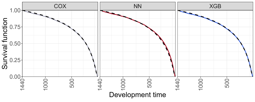
Figure 4: Scenario Alpha, claim_type 1 and AD 13. The true survival function (black dotted line) is compared to the fitted survival function with COX, NN, and XGB (left to right).

In Figure 4 we show the true survival function compared to the fitted survival function in scenario Alpha. It can be noticed that all the three models seem to behave consistently with respect to the true curve. Interestingly, even in the simplest modeling scenario, XGB and COX seem to be better than NN in catching the behavior of the survival function on the right tail.

The same plot can be shown for other scenarios. An interesting case is scenario Delta, where we introduced a seasonality effect dependent on the accident period, see again Table 1. In this section we first show the feature combination claim_type 1 and AD 691 where the three models seem to behave similarly with XGB closer to the true survival function, see Figure 5.

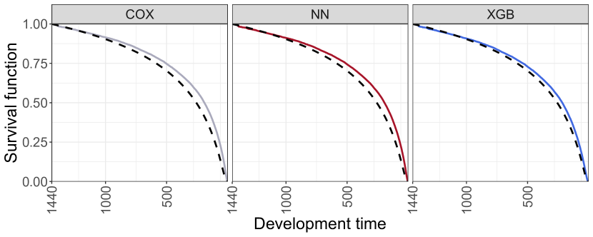
Figure 5: Scenario Delta, claim_type 1 and AD 691. The true survival function (black dotted line) is compared to the fitted survival function with COX, NN, and XGB (left to right).

6.4 Results: forecasting using the development factors

In this section we compare the chain ladder with our models in the five simulated scenarios. In each scenario, we simulate $20$ data sets to show that our results are not affected from accidental fluctuations of the simulations. Below we describe in brief the procedure that we used.

1. For each scenario (Alpha, Beta, Gamma, Delta, and Epsilon), we simulate $20$ data set.

2. On each data set, we find the optimal hyper parameters for NN and XGB using Bayesian optimization Snoek . (2012). More details on the optimization algorithm can be found in Appendix A.

3. On each data set, we fit COX and the optimal NN and XGB.

4. We find the estimated development factors and expected number of future occurrences according to each model.

5. We evaluate the performances for COX, NN, and XGB using the $\texttt{ARE}^{\texttt{TOT}}$, the CRPS and the $\texttt{ARE}^{\texttt{CAL}}$ on a quarterly and yearly basis. The $\texttt{ARE}^{\texttt{TOT}}$ and $\texttt{ARE}^{\texttt{CAL}}$ are also computed for the CL.

6. For each scenario we report the average performance measures of CL, COX, NN, and XGB over the 20 data sets.

Model	Scenario	$\texttt{ARE}^{\texttt{TOT}}$	$\texttt{ARE}^{\texttt{CAL}}$ (quarters)	$\texttt{ARE}^{\texttt{CAL}}$ (years)	CRPS
CL (✓)	Alpha	0.131 ($\pm$ 0.016)	0.128 ($\pm$ 0.014)	0.037 ($\pm$ 0.011)	-
COX (✓)		0.138 ($\pm$ 0.013)	0.131 ($\pm$ 0.012)	0.044 ($\pm$ 0.013)	364.428 ($\pm$ 5.899)
NN (✓)		0.140 ($\pm$ 0.021)	0.132 ($\pm$ 0.015)	0.045 ($\pm$ 0.015)	366.902 ($\pm$ 8.567)
XGB (✓)		0.136 ($\pm$ 0.010)	0.131 ($\pm$ 0.011)	0.042 ($\pm$ 0.012)	364.230 ($\pm$ 5.967)
CL (✗)	Beta	0.215 ($\pm$ 0.023)	0.194 ($\pm$ 0.015)	0.122 ($\pm$ 0.025)	-
COX (✓)		0.162 ($\pm$ 0.014)	0.161 ($\pm$ 0.011)	0.050 ($\pm$ 0.018)	402.794 ($\pm$ 6.929)
NN (✓)		0.169 ($\pm$ 0.019)	0.166 ($\pm$ 0.015)	0.062 ($\pm$ 0.028)	403.057 ($\pm$ 7.720)
XGB (✓)		0.162 ($\pm$ 0.013)	0.162 ($\pm$ 0.011)	0.048 ($\pm$ 0.019)	402.343 ($\pm$ 7.133)
CL (✗)	Gamma	0.260 ($\pm$ 0.035)	0.230 ($\pm$ 0.029)	0.191 ($\pm$ 0.032)	-
COX (✗)		0.147 ($\pm$ 0.015)	0.149 ($\pm$ 0.013)	0.057 ($\pm$ 0.022)	402.917 ($\pm$ 6.221)
NN (✓)		0.167 ($\pm$ 0.044)	0.160 ($\pm$ 0.027)	0.075 ($\pm$ 0.039)	402.311 ($\pm$ 9.258)
XGB (✓)		0.154 ($\pm$ 0.024)	0.147 ($\pm$ 0.018)	0.053 ($\pm$ 0.025)	401.996 ($\pm$ 5.988)
CL (✗)	Delta	0.300 ($\pm$ 0.024)	0.234 ($\pm$ 0.018)	0.037 ($\pm$ 0.012)	-
COX(✓)		0.195 ($\pm$ 0.022)	0.192 ($\pm$ 0.018)	0.065 ($\pm$ 0.020)	386.598 ($\pm$ 6.667)
NN (✓)		0.213 ($\pm$ 0.034)	0.204 ($\pm$ 0.025)	0.051 ($\pm$ 0.023)	388.707 ($\pm$ 7.205)
XGB (✓)		0.167 ($\pm$ 0.019 )	0.145 ($\pm$ 0.011)	0.058 ($\pm$ 0.025)	369.531 ($\pm$ 6.599)
CL (✓)	Epsilon	0.119 ($\pm$ 0.011)	0.115 ($\pm$ 0.010)	0.035 ($\pm$ 0.010)	-
COX (✗)		0.135 ($\pm$ 0.022)	0.127 ($\pm$ 0.010)	0.060 ($\pm$ 0.015)	340.267 ($\pm$ 5.192)
NN (✗)		0.132 ($\pm$ 0.015)	0.126 ($\pm$ 0.011)	0.059 ($\pm$ 0.019)	341.169 ($\pm$ 5.210)
XGB (✗)		0.149 ($\pm$ 0.059)	0.127 ($\pm$ 0.012)	0.057 ($\pm$ 0.017)	340.344 ($\pm$ 5.100)

Table 3: Results after 20 simulations. We show the different performance measure for our different models (column one). In the different scenarios (column two) the models assumptions might be not satisfied. We indicate with a check mark (✓) the scenarios in which the models assumptions are satisfied. For each model we also display the performance measures we described in the previous sections: absolute total reserving error (column three), absolute error by diagonal for quarterly output (column four) and absolute relative error by diagonal for yearly output (column five). Between brackets, we show the standard deviation of the (average) performance measures over the 20 records. In column six we show the continuously ranked probability score.

The results of the data application on simulated data are summarized in Table 3. In column one, we list the models included in the comparison for each scenario (column two). Similarly to Table 1, we denote with a check mark or an x mark if the model assumptions are satisfied or not. Let us first consider the comparison with CL in terms of $\texttt{ARE}^{\texttt{TOT}}$ and $\texttt{ARE}^{\texttt{CAL}}$. Our data application shows that CL is outperforming the individual models in scenario Alpha and in scenario Epsilon according to the $\texttt{ARE}^{\texttt{TOT}}$ and the $\texttt{ARE}^{\texttt{CAL}}$. In scenario Alpha, the CL results are very close to those of COX, NN, and XGB. As expected, in scenario Epsilon, breaking down the proportionality assumption, the CL is better than the other models. Interestingly, when we inspect the most complex scenarios (Beta, Gamma, and Delta) our approach (COX, NN, and XGB) provides better scores than the CL model. Notably, we observe that XGB is consistently the best performing model. Notwithstanding the intensive hyper parameters tuning that we performed, NN seem to perform worse than COX in most scenarios. In scenario Delta, where we introduce a seasonality effect we find that according to all the proposed scores XGB is by far the best model. The $\texttt{ARE}^{\texttt{TOT}}$ and $\texttt{ARE}^{\texttt{CAL}}$ are a good benchmark to compare our approach to the CL but they are not proper scoring rules. Conversely, we can take the CRPS as the main criterion to rank our models. In the scenarios we considered, the CRPS indicates that XGB is outperforming NN and COX. Interestingly, while in scenarios Alpha, Beta, Gamma, and Epsilon the XGB (average) CRPS is close to COX, in scenario Delta we observe a major drop in the CRPS going from COX to XGB. In scenario Gamma we find that the NN model performs better than COX. Interestingly, in this scenario the COX assumptions are not satisfied.

6.4.1 A cell-wise comparison

In this section, we provide a heat map of the average relative prediction error of the $k,j$ cells over the simulations for each scenario on a quarterly basis. In particular, we want to detect whether the IBNR frequencies predicted for the $k,j$ cells are overestimated or underestimated. In this phase we can detect if paths are present in the models results extrapolation.

The relative error $\texttt{RE}^{k,j}$ for the $k,j$ cell of some development triangle is

$$\texttt{RE}^{k,j}=\frac{\sum_{x}O^{\prime}_{k,j}(x)-\sum_{x}\hat{O}^{\prime}_{k,j}(x)}{\sum_{x}O^{\prime}_{k,j}(x)}.$$ (10)

In Figure 6 we show a heat map of the average $\texttt{RE}^{k,j}$ over the simulated data sets of each model in each scenario. For all the scenarios that we investigated, our models seem to reduce the relative errors within the cells. Cell-wise, XGB models residuals are the closest to zero. An interesting insight comes from scenario Delta. We recall that in scenario Delta we simulated the data with a seasonality effect. Interestingly, the XGB model is the only model able to catch the seasonality effect in scenario Delta. Surprisingly, the NN model is not capable of catching the interactions with the accident period notwithstanding the heavy hyper parameters tuning procedure, see Appendix A.

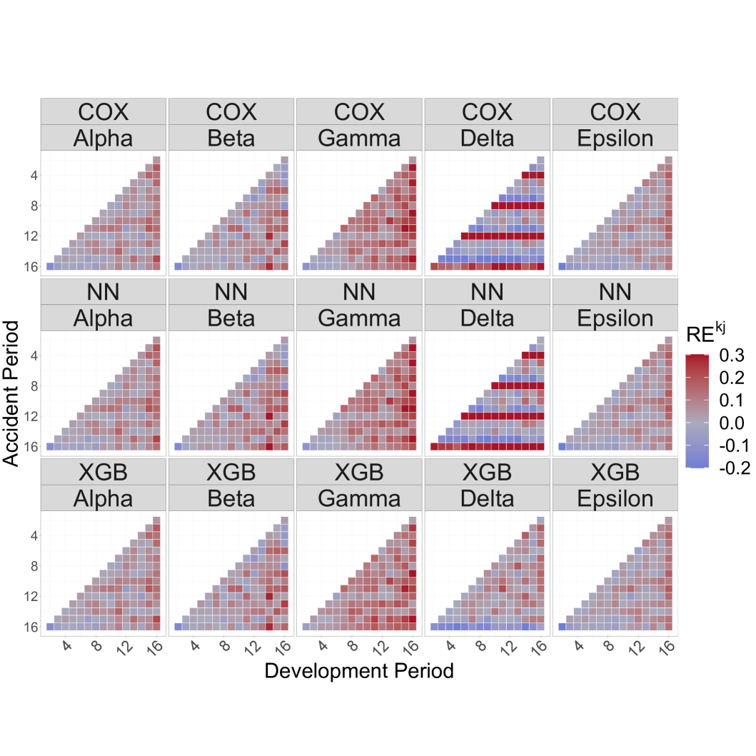
Figure 6: The average (over the simulations) of the relative errors: $\frac{\sum_{x}O_{k,j}(x)-\sum_{x}\hat{O}_{k,j}(x)}{\sum_{x}O_{k,j}(x)}$

7 Data application on real data

In this section we show a case study based on a real data set from Codan Forsikring. We had at disposal the company complete reserving data from $2012$ to $2022$ for a short tailed personal line product. Two categorical features are associated to each (claim claim_type and coverage_key). The complete description of the data set is available in Table 4.

Features	Description
Claim_number	Policy identifier.
claim_type $\in\left\{1,\ldots,20\right\}$	Type of claim.
coverage_key $\in\left\{1,\ldots,16\right\}$	Type of coverage.
AM	Accident month.
CM	Calendar month of report.
DM	Development month.
incPaid	Incremental paid amount. We will not use this information in the manuscript.

Table 4: Description of the Codan Forsikring data set.

We decided to split the data into $6$ chunks of $5$ consecutive years each. The splits are reported in Table 5, together with the corresponding data size. For each of these splits, we fit our models on the first $4$ years (train data) and score our models on the fifth year (test data).

	Training	Scoring	Train data size (observations number)	Test data size (observations number)	Mean Reporting Delay
Split 1	2012-2016	2017	129381	1474	1.62
Split 2	2013-2017	2018	133367	1553	1.62
Split 3	2014-2018	2019	130405	1566	1.63
Split 4	2015-2019	2020	122842	1394	1.63
Split 5	2016-2020	2021	110884	1225	1.61
Split 6	2017-2021	2022	105618	1069	1.55

Table 5: For each split (column one) we reported the accident periods we used to train the models (column two), and the year we use for scoring (column three). In columns four and five we show the train and test data size. In column six we provide the mean reporting delay from accident.

Similarly to the case study on the simulated data, we compare our results with the chain ladder model fitted on a quarterly and yearly grid. We fitted our models on a monthly grid, according to the procedure we described in the manuscript. In Table 5, we show the mean reporting delay in each data split. Most of the notifications occurred in the early development periods and the mean reporting delay is between one and two months showing that the data are very stable.

From Figure 7 we can see that not all the combinations of the two categorical features (cover_key and claim_type_key) were observed (see Figure 7). Most of the data belong to the combinations claim_type_key 1 with cover_key 1 and cover_key 5 and claim_type_key 14 with cover_key 1.

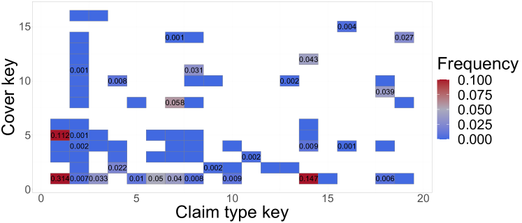
Figure 7: Relative frequency on the complete data ($2012-2021$). We do not observe all the combinations of features and most of the data show claim_type_key 1, and cover_key 1 or cover_key 5.

7.1 Results

In Table 6 we show the our models performance on the real data splits described in Table 5. The models are reported in column one and the data splits are reported in column two. In this setting, the chain ladder is expect to perform very well as the data have are reported in the early development months and, from the authors experience on this data sets, there are few reports in the late development periods. Interestingly, from the results of the $\texttt{ARE}^{\texttt{TOT}}$ and $\texttt{ARE}^{\texttt{CAL}}$ (columns three to five) we see that in general we have an improvement in the models performance using COX, NN, or XGB compared to the CL, especially in terms of $\texttt{ARE}^{\texttt{CAL}}$. By comparing COX, NN and XGB we obtain further insights on the performance of our models. The $l(\theta)$ results (columns six and seven) indicate that XGB is the best model in minimizing the objective function, both in-sample and out-of-sample . Similarly to the simulated scenarios, we randomly split our data into training and validation for fitting NN and XGB. With the same rule of thumb we also kept the $80\%$ of the data for training. As highlighted in the previous sections, the CRPS is our main criterion to select a model the best performing model. The CRPS suggests that in the first three data splits, NN and XGB outperform the COX model. In general, we observe that COX is the best performing model. This is also enforced from the other performance measures $\texttt{ARE}^{\texttt{TOT}}$ and $\texttt{ARE}^{\texttt{CAL}}$. The motivation for these results is related to the behavior of the data set. We already discussed that there are no complex trends in our data, meaning that there is a benefit in using our modeling approach compared to the CL but the simplest hazard model (COX) is the most accurate based on the performance measures that we defined.

Model	Split	$\texttt{ARE}^{\texttt{TOT}}$	$\texttt{ARE}^{\texttt{CAL}}$ (quarters)	$\texttt{ARE}^{\texttt{CAL}}$ (years)	CRPS	$l(\theta)$ (in-sample)	$l(\theta)$ (out-of-sample)
CL	Split 1	0.207	0.225	0.264
COX		0.242	0.208	0.242	6.429	10.781
NN		0.241	0.206	0.237	6.420	10.531	9.144
XGB		0.231	0.202	0.235	6.440	10.529	9.143
CL	Split 2	0.235	0.323	0.155
COX		0.307	0.296	0.082	8.061	10.804
NN		0.307	0.296	0.084	8.054	10.551	9.165
XGB		0.287	0.292	0.100	8.074	10.549	9.163
CL	Split 3	0.262	0.324	0.196
COX		0.306	0.268	0.069	6.303	10.784
NN		0.297	0.261	0.059	6.496	10.528	9.141
XGB		0.324	0.286	0.081	6.468	10.522	9.138
CL	Split 4	0.213	0.264	0.181
COX		0.270	0.248	0.081	6.076	10.725
NN		0.283	0.258	0.082	5.950	10.475	9.089
XGB		0.282	0.254	0.088	6.220	10.463	9.077
CL	Split 5	0.203	0.193	0.064
COX		0.160	0.181	0.107	4.855	10.623
NN		0.171	0.188	0.111	5.017	10.371	8.985
XGB		0.169	0.182	0.102	5.012	10.357	8.972
CL	Split 6	0.198	0.177	0.219
COX		0.196	0.187	0.176	4.321	10.576
NN		0.196	0.186	0.180	4.342	10.318	8.931
XGB		0.200	0.186	0.168	4.368	10.313	8.926

Table 6: Results on the case study on real data. For each model (column one) and in each data split (column two) we show the results of $\texttt{ARE}^{\texttt{TOT}}$ (column three), $\texttt{ARE}^{\texttt{CAL}}$ (columns four and five), the in-sample and out-of-sample likelihood (columns six and seven) and the CRPS (column eight). The $\texttt{ARE}^{\texttt{CAL}}$ is presented quarterly and yearly in columns four and five respectively.

7.2 Sensitivities

Inspired by the analysis of the sensitivities in wuthrich18, we show that for a fixed combination of features and a fixed development period, the marginal effect of the different levels of a model features on the development factors for Spit 1. The benchmark is the development factor modelled with the chain ladder. The first row shows our results on a quarterly grid (Figure 8(a), Figure 8(b), Figure 8(c)) for the second development quarter. In Figure 8(a) fix the accident quarter to $16$, and cover_key to $1$ and let claim_type_key vary. In Figure 8(b), we pick cover_key 1, claim_type_key 1 and let the accident quarter change. In Figure 8(c), we pick accident quarter $16$, claim_type_key 1 and let the cover_key.

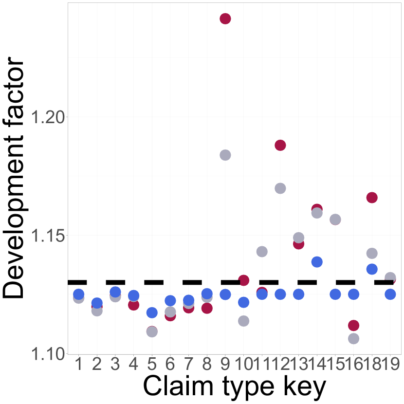
(a)

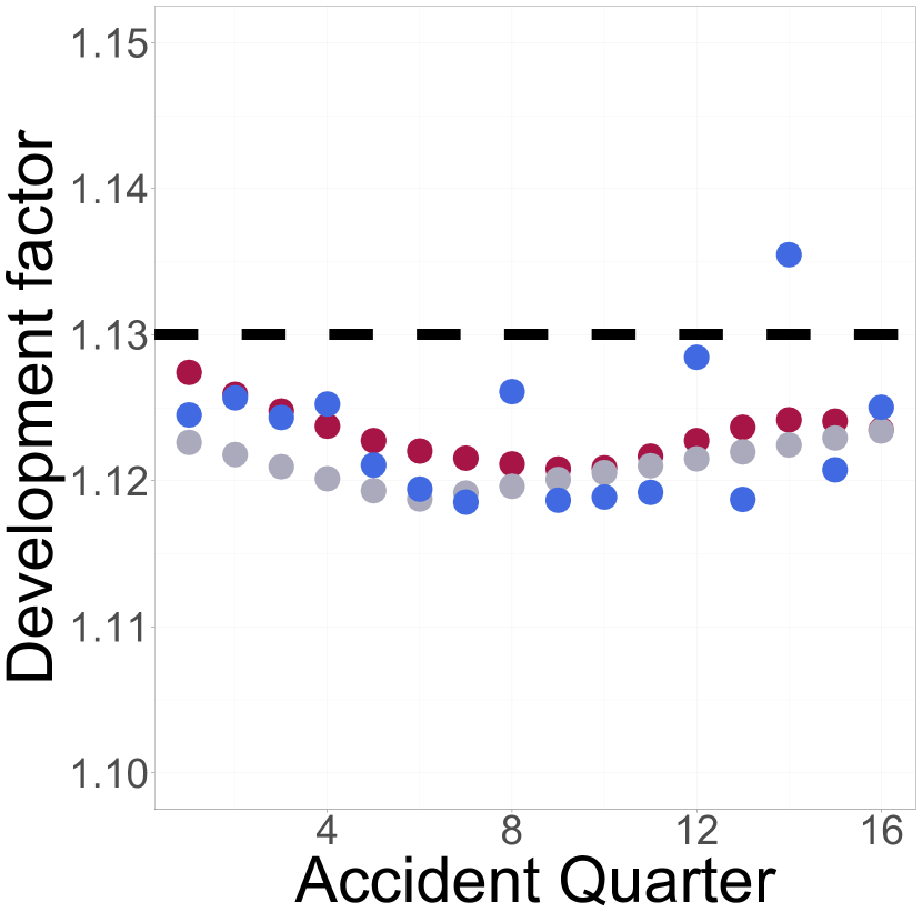
(b)

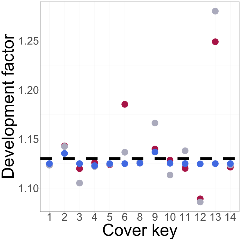
(c)

Figure 8: Development factor $2$ sensitivity for the quarterly output in Split 6. The dotted line represents the chain ladder estimate. The dots indicate the estimates from the different models: COX (red), NN (gray) and XGB (blue).

In a similar fashion, in Figure 9 we show a similar plot for the yearly results. In Figure 9(a) we fix the accident year to $4$, and cover_key to $1$ and let claim_type_key vary. In Figure 9(b), we pick cover_key 1, claim_type_key 1 and let the accident quarter change. In Figure 9(c), we pick accident quarter $4$, claim_type_key 1 and let the cover_key.

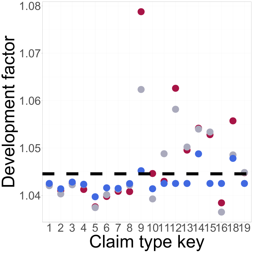
(a)

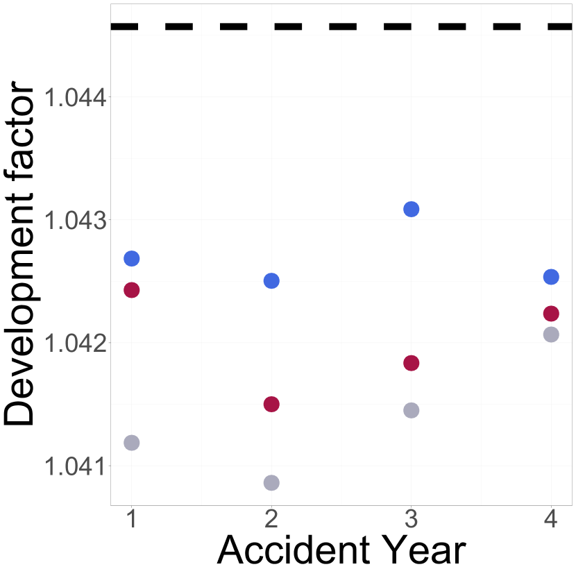
(b)

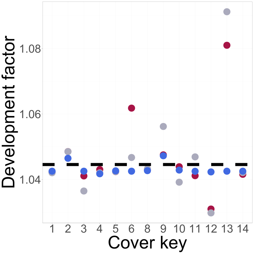
(c)

Figure 9: Development factor $2$ sensitivity for the yearly output in Split 6. The dotted line represents the chain ladder estimate. The dots indicate the estimates from the different models: COX (red), NN (gray) and XGB (blue).

8 Concluding remarks

Based on the work of Miranda . (2013) and Hiabu (2017), we introduced a survival analysis framework to use machine learning techniques to estimate development factors that can depend on accident date and other features. The approach presented in this paper has been developed with the aim to give higher accuracy in cases where more information in form of individual claims data is available while at the same time conserving the structure reserving actuaries are used to. Our extensive simulation study suggests that our methodology does indeed seem to work well. In this paper, we have only considered the prediction of IBNR counts and an obvious next step is to integrate our methodology into a wider framework to estimate the outstanding claims amount. It could for example be interesting to merge our approach with recent RBNS prediction methods like Crevecoeur . (2022) or Lopez  Milhaud (2021).

9 Supplementary material

The code at gpitt71/resurv-replication-code complements the results of this manuscript and can be used to replicate the case study of Section 6. The GitHub folder resurv-replication-code, was registered with a unique Zenodo DOI. The code to obtain the plots that we included in the manuscript can be found in the package vignette Manuscript replication material of edhofman/ReSurv. Also the GitHub folder ReSurv, was registered with a unique Zenodo DOI.

Appendix A Bayesian optimization of machine learning algorithms

In this paper we showed an extended analysis of $5$ simulated scenarios and a case study where we use machine learning to process large data sets and catch complex interactions in the data. Machine learning algorithms are very sensitive to the parameters and hyper parameters choice ([p. 219]hastie09, []snoek12). In this section, we provide general details about the strategy that we used for the hyper parameters selection of NN and XGB. Optimizing the algorithms over many data sets might lead to protracted computational times, Jones (2001). As a solution, we use the Bayesian optimization procedure described in snoek12. While grid searches can be cumbersome for big searches, using the approach in Snoek . (2012) we use the information from prior model evaluations to guide the optimal parameters search. Notably, Bayesian optimization methods have shown to be well-performing in challenging optimization problems Jones (2001).

Let us consider the data $\left\{(x_{i},y_{i})\right\}_{i=1,\ldots,n}$. In this setting, the functional relationship between input and output $h:X\rightarrow\mathbb{R}$ is modelled as:

$$y_{n}\sim\mathcal{N}\left(h(x_{n}),\nu\right),$$

with $\nu$ being the variance of noise introduced into the function observations. Furthermore, let us assume that the observations $h\left(x\right)$ are drawn from a Gaussian prior.

Under the Gaussian Process prior, we get a posterior function (i.e., $a$ acquisition function) $a:X\rightarrow\mathbb{R}^{+}$ that depends on the model solely through its predictive mean function $\mu(x;\left\{(x_{i},y_{i})\right\}_{i},\theta)$ and predictive variance function $\sigma^{2}(x;\left\{(x_{i},y_{i})\right\}_{i},\theta)$. Conversely, the acquisition function depends on the previous observations, as well as the Gaussian Process hyperparameters $a(x;\left\{(x_{i},y_{i})\right\}_{i},\theta)$. In order to avoid an involved notation we denote

• $a(x;\left\{(x_{i},y_{i})\right\}_{i},\theta)$ as $a\left(x\right)$

• $\mu(x;\left\{(x_{i},y_{i})\right\}_{i},\theta)$ as $\mu\left(x\right)$

• $\sigma^{2}(x;\left\{(x_{i},y_{i})\right\}_{i},\theta)$ as $\sigma^{2}\left(x\right)$

There are different definitions for the acquisition function Snoek . (2012), we choose

$$a\left(x\right)=\left(\mu(x)-h_{\max}\right)\Phi\left(\frac{\mu(x)-h_{\max}-\xi}{\sigma(x)}\right)+\sigma(x)\phi\left(\frac{\mu(x)-h_{\max}-\xi}{\sigma(x)}\right),$$ (11)

where

• $h_{\max}$ is the current maximum value obtained from sampling.

• $\Phi$ is the standard normal cumulative density function.

• $\phi$ is the standard normal probability density function.

• $\xi$ is an exploration parameter Wilson (2022).

This approach for Bayesian optimization is described with the following steps:

1. Set the parameters to an initial value.

2. Fit the Gaussian process.

3. Find the parameters that maximize the acquisition function.

4. Score the parameter.

5. Repeat steps 2-4 until some stopping criteria is met Snoek . (2012).

A thorough description can be found in Snoek . (2012). We show the hyperparameters we inspected for each model in Table 7.

Model	hyperparameter	Range
NN	num_layers	$\left[2,10\right]$
	num_nodes	$\left[2,10\right]$
	optim	$\left[1,2\right]$
	activation	$\left[1,2\right]$
	lr	$\left[.005,0.5\right]$
	xi	$\left[0,0.5\right]$
	eps	$\left[0,0.5\right]$
XGB	eta	$\left[0,1\right]$
	max_depth	$\left[0,25\right]$
	min_child_weight	$\left[0,50\right]$
	subsample	$\left[0.1,1\right]$
	lambda	$\left[0,50\right]$
	alpha	$\left[0,50\right]$

Table 7: The range of hyperparameters we inspected. We set the same ranges for the $5$ simulations and the case study on the real data.

Below we disclose the computational times we required for fitting the parameters combinations on the five simulated scenarios (Table 8) and the real data (Table 9).

Model	Scenario	Hyperparameter selection	Model fit
COX	Alpha		3.20
NN		52.57	149.31
XGB		3.19	16.77
COX	Beta		2.49
NN		44.00	102.13
XGB		2.83	15.66
COX	Gamma		2.25
NN		68.72	204.58
XGB		5.10	21.91
COX	Delta		2.23
NN		75.05	132.79
XGB		8.72	19.61
COX	Epsilon		1.94
NN		66.33	109.64
XGB		3.51	11.43

Table 8: Average computational times in minutes, simulated scenarios. Hyperparameters selection is on 3-folded cross validation. Model fit includes development factor fitting.

Model	Split	Hyperparameter selection	Model fit
COX	Split 1		1.53
NN		88.28	27.18
XGB		10.57	21.56
COX	Split 2		1.37
NN		93.30	32.41
XGB		31.25	24.06
COX	Split 3		0.94
NN		161.71	40.91
XGB		19.01	25.86
COX	Split 4		1.80
NN		107.15	38.28
XGB		65.10	28.01
COX	Split 5		1.74
NN		115.49	20.78
XGB		38.12	26.80
COX	Split 6		1.24
NN		87.51	19.99
XGB		35.45	27.38

Table 9: Computational times in minutes, real data. Hyperparameters selection is on 3-folded cross validation. Model fit includes development factor fitting.

Appendix B Scenarios simulation

In section 6 we illustrated the steps that we followed to generate the five simulated scenarios. We also mentioned that the parametrization of $\phi(x,u;\theta)$ changes for the different scenarios. In this section we want to provide extra details on the parameters that we used in the simulation phase. For the data generation we will only need two modules from the SynthETIC package, i.e. the number of claims occurring every accident date and the reporting delay. In every scenario for both claim types, the rate of claims occurrence is $.2$. In scenarios Alpha, Gamma, Delta, and Epsilon the individuals at risk in the portfolio are $200$ in each accident date. In scenario Beta the individuals for claim_type 1 are decreasing. The relative portfolio composition is shown in Figure 10(a) and Figure 10(b).

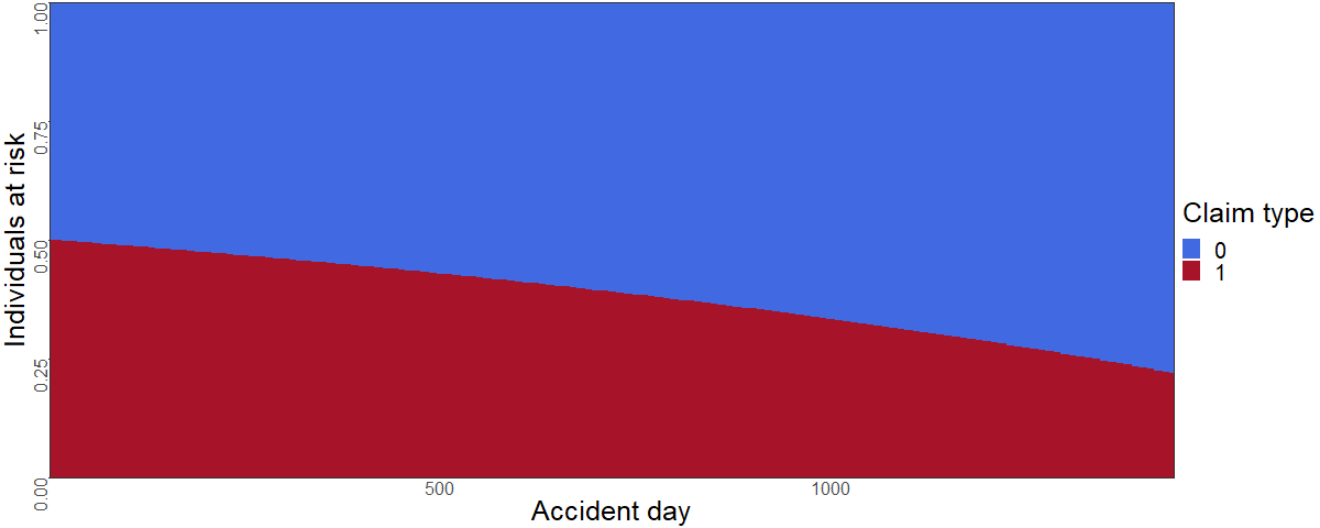
(a) Portfolio composition by claim_type for each accident date (AD $\in\left\{1,\ldots,1440\right\}$) in scenarios Alpha, Gamma, Delta and Epsilon.

(b) Portfolio composition by claim_type for each accident date (AD $\in\left\{1,\ldots,1440\right\}$) in scenario Beta.

Figure 10: In scenarios Alpha, Gamma, Delta, and Epsilon the portfolio is composed of half claim_type 0 claims and half claim_type 1 claims. In scenario Beta the individuals at risk for claim_type 1 decrease for the most recent accident dates.

In Table 10 we report the parameters that we used to simulate from the RTFWD distribution in Teamah . (2019). We recall that the RTFWD has a four parameter structure $\nu,\pi,\xi,k$, and is defined with $0<t\leq b$ with cumulative distribution function

$$F(t)=\exp(-\pi^{\nu}\xi^{\nu k}(t^{-\nu k}-b^{-\nu k})).$$

Scenario	$\nu$	$\pi$	$k$	$\xi_{0}$
Alfa, Beta, Gamma, Delta	0.5	60	1	0.1
Epsilon	0.5	$60+(34.5387\mathbbm{1}_{\texttt{claim\_type ==0}}+58.6803\mathbbm{1}_{\texttt{claim\_type ==0}})$	1	0.1

Table 10: The RTFWD distribution parameters (columns two to four) for the different scenarios (column one).

In Table 11 we reported the parameters that we used for the simulation of the hazard. In the scenarios Alpha, Beta, Gamma, and Delta the reverse time hazard has the form

$$\alpha(t|\text{{claim\_type}},\text{{AD}})=\alpha_{0}(t)e^{\phi\left(\text{{claim\_type}},\text{{AD}};\theta\right)}$$

In column two of Panel A of Table 11 we show the baseline $\alpha_{0}(t)$. We highlight that $\alpha_{0}(t)$ is the same for the five scenarios. In column three of panel A we show the different effects of the features on the proportional risk $e^{\phi\left(\text{{claim\_type}},\text{{AD}};\theta\right)}$ for the different scenarios (column 1).

In scenario Epsilon the hazard is not generated from a proportional model and it has the form:

$$\alpha(t|\text{{claim\_type}},\text{{AD}})=\alpha_{0}(t|\text{{claim\_type}})(\exp(\phi\left(\text{{claim\_type}},\text{{AD}};\theta\right))+f(\texttt{claim\_type})).$$

Details on the simulation for this scenario are provided in Panel B of Table 11. In Panel C we show the coefficients values that we chose to simulate the proportional risk for the different scenarios (columns one to seven).

Table 11: The parameters that we used for the reverse hazard simulation in the different scenarios. Baseline (column two) and effects on the proportional risk (column three) for the five scenarios (column one). Let us define $I(\text{{AD}})=\text{{AD}}-30\%(\text{{AD}}-1)/30\rfloor$

Scenario	$\alpha_{0}(t)$	$\phi\left(\text{{claim\_type}},\text{{AD}};\theta\right)$
Alpha	$0.5\sqrt{0.2t^{-1}}$	$\beta_{0}\mathbbm{1}_{\texttt{claim\_type ==0}}+\beta_{1}\mathbbm{1}_{\texttt{claim\_type ==1}}$
Beta		$\beta_{0}\mathbbm{1}_{\texttt{claim\_type ==0}}+\beta_{1}\mathbbm{1}_{\texttt{claim\_type ==1}}$
Gamma		$\beta_{0}\mathbbm{1}_{\texttt{claim\_type ==0}}+\beta_{1}\mathbbm{1}_{\texttt{claim\_type ==1}}+\beta_{2}\mathbbm{1}_{\texttt{claim\_type ==1}}\sqrt{\text{{AD}}}$
Delta		$\beta_{0}\mathbbm{1}_{\texttt{claim\_type ==0}}+\beta_{1}\mathbbm{1}_{\texttt{claim\_type ==1}}+\beta_{3}\mathbbm{1}_{I(\text{{AD}})\in\left\{2,3,4\right\}}$ $+\beta_{4}\mathbbm{1}_{I(\text{{AD}})\in\left\{5,6,7\right\}}+\beta_{5}\mathbbm{1}_{I(\text{{AD}})\in\left\{8,9,10\right\}}+\beta_{6}\mathbbm{1}_{I(\text{{AD}})\in\left\{11,0,1\right\}}$

Scenario	$f(\text{{claim\_type}})$	$\alpha_{0}(t|\text{{claim\_type}})$	$\phi\left(\text{{claim\_type}},\text{{AD}};\theta\right)$
Epsilon	$0.5\phi\left(\text{{claim\_type}},\text{{AD}};\theta\right)$	$0.5\sqrt{0.1(2+f(x)))t^{-1}}$	$\beta_{0}\mathbbm{1}_{\texttt{claim\_type ==0}}+\beta_{1}\mathbbm{1}_{\texttt{claim\_type ==1}}$

Table 12: Panel B: Baseline (column three), effects on $\phi\left(\text{{claim\_type}},\text{{AD}};\theta\right)$ (column four) and $f(\text{{claim\_type}})$ for scenario Epsilon (column one).

$\beta_{0}$	$\beta_{1}$	$\beta_{2}$	$\beta_{3}$	$\beta_{4}$	$\beta_{5}$	$\beta_{6}$
$1.1512$	$1.95601$	$-0.021206$	$-0.3$	$0.4$	$-0.7$	$0.1$

Table 13: Panel C: Features effects, $\beta_{0},\ldots\beta_{6}\in\mathbb{R}$

Appendix C Minimizing the log-likelihood

In this section we will show the hazard models average in-sample negative partial log-likelihood, i.e. the loss function we minimize during the models training computed on the data that we used to fit the models. In order to ease our notation, we will indicate the average negative log-likelihood in Equation 3 as $l$. The model with the minimum in-sample average negative partial log-likelihood is the model that fits best the training data. We train the COX model using all the individual data from calendar periods $\tau=1,\ldots,\mathcal{T}$. In the training phase of XGB and NN, the input data from calendar periods $\tau=1,\ldots,\mathcal{T}$ are further split into a main part for training and a smaller part for validation. The split is random and we use $80\%$ of the data for training (the splitting percentage is selected with a rule of thumb). We will then report for XGB and NN the out-of-sample average negative log-likelihood measured on the remaining $20\%$ of the input data. Comparing the in-sample likelihood and the out-of-sample likelihood will tell us whether a model is overfitting the data. Indeed, we expect that a) the models can be ordered in the same way based on their descending score in-sample and out-of-sample and b) the magnitude of the scores in-sample and out-of-sample is comparable. In Table 2 we show the (average) negative log-likelihood averaged (over the $20$ simulations), for each model in each scenario. The results show that XGB and NN seem to best fit the in-sample data compared to COX. Furthermore, XGB is consistently providing a lower likelihood compared to the NN. A similar behavior is reflected in the out-of-sample data.

A similar table can be provided for the real world data application Table 6.

Appendix D Computational details

The computations were performed in Linux, using ERDA (Electronic Research Data Archive, University of Copenhagen). The relevant computational details on the architecture are provided below.

⬇

>>> lscpu

Architecture: x86_64

CPU op-mode(s): 32-bit, 64-bit

Address sizes: 48 bits physical, 48 bits virtual

Byte Order: Little Endian

CPU(s): 64

On-line CPU(s) list: 0-63

Vendor ID: AuthenticAMD

Model name: AMD EPYC Processor (with IBPB)

CPU family: 23

Model: 1

Thread(s) per core: 1

Core(s) per socket: 1

Socket(s): 64

Stepping: 2

BogoMIPS: 4000.00

References

- Aalen (\APACyear1978) \APACinsertmetastaraalen78{APACrefauthors}Aalen, O\BPBIO. \APACrefYearMonthDay1978. \BBOQ\APACrefatitleNonparametric Inference for a Family of Counting Processes Nonparametric inference for a family of counting processes.\BBCQ \APACjournalVolNumPagesThe Annals of Statistics64701–726. \PrintBackRefs\CurrentBib
- Ajne (\APACyear1994) \APACinsertmetastarajne94{APACrefauthors}Ajne, B. \APACrefYearMonthDay1994. \BBOQ\APACrefatitleAdditivity of Chain-Ladder Projections Additivity of chain-ladder projections.\BBCQ \APACjournalVolNumPagesASTIN Bulletin242311–318. \PrintBackRefs\CurrentBib
- Andersen \BOthers. (\APACyear2012) \APACinsertmetastarandersen12{APACrefauthors}Andersen, P\BPBIK., Borgan, O., Gill, R\BPBID.\BCBL \BBA Keiding, N. \APACrefYear2012. \APACrefbtitleStatistical models based on counting processes Statistical models based on counting processes. \APACaddressPublisherSpringer Science & Business Media. \PrintBackRefs\CurrentBib
- Avanzi \BOthers. (\APACyear2021) \APACinsertmetastarAvanzi21{APACrefauthors}Avanzi, B., Taylor, G., Wang, M.\BCBL \BBA Wong, B. \APACrefYearMonthDay2021sep. \BBOQ\APACrefatitleSynthETIC: An individual insurance claim simulator with feature control SynthETIC: An individual insurance claim simulator with feature control.\BBCQ \APACjournalVolNumPagesInsurance: Mathematics and Economics100296–308. \PrintBackRefs\CurrentBib
- Bischofberger \BOthers. (\APACyear2020) \APACinsertmetastarbischofberger20{APACrefauthors}Bischofberger, S\BPBIM., Hiabu, M.\BCBL \BBA Isakson, A. \APACrefYearMonthDay2020. \BBOQ\APACrefatitleContinuous chain-ladder with paid data Continuous chain-ladder with paid data.\BBCQ \APACjournalVolNumPagesScandinavian Actuarial Journal20206477–502. \PrintBackRefs\CurrentBib
- Bischofberger \BOthers. (\APACyear2019) \APACinsertmetastarbischofberger2019comparison{APACrefauthors}Bischofberger, S\BPBIM., Hiabu, M., Mammen, E.\BCBL \BBA Nielsen, J\BPBIP. \APACrefYearMonthDay2019. \BBOQ\APACrefatitleA comparison of in-sample forecasting methods A comparison of in-sample forecasting methods.\BBCQ \APACjournalVolNumPagesComputational Statistics & Data Analysis137133–154. \PrintBackRefs\CurrentBib
- Breslow (\APACyear1974) \APACinsertmetastarbreslow74{APACrefauthors}Breslow, N. \APACrefYearMonthDay1974. \BBOQ\APACrefatitleCovariance analysis of censored survival data Covariance analysis of censored survival data.\BBCQ \APACjournalVolNumPagesBiometrics89–99. \PrintBackRefs\CurrentBib
- Calcetero-Vanegas \BOthers. (\APACyear2023) \APACinsertmetastarcalcetero2023claim{APACrefauthors}Calcetero-Vanegas, S., Badescu, A\BPBIL.\BCBL \BBA Lin, X\BPBIS. \APACrefYearMonthDay2023. \BBOQ\APACrefatitleClaim Reserving via Inverse Probability Weighting: A Micro-Level Chain-Ladder Method Claim reserving via inverse probability weighting: A micro-level chain-ladder method.\BBCQ \APACjournalVolNumPagesarXiv preprint arXiv:2307.10808. \PrintBackRefs\CurrentBib
- Chen \BBA Guestrin (\APACyear2016) \APACinsertmetastarchen16{APACrefauthors}Chen, T.\BCBT \BBA Guestrin, C. \APACrefYearMonthDay2016. \BBOQ\APACrefatitleXGBoost: A Scalable Tree Boosting System XGBoost: A scalable tree boosting system.\BBCQ \BIn \APACrefbtitleProceedings of the 22nd ACM SIGKDD International Conference on Knowledge Discovery and Data Mining Proceedings of the 22nd acm sigkdd international conference on knowledge discovery and data mining (\BPGS 785–794). \APACaddressPublisherNew York, NY, USAACM. {APACrefURL} http://doi.acm.org/10.1145/2939672.2939785 {APACrefDOI} \doi10.1145/2939672.2939785 \PrintBackRefs\CurrentBib
- Cox (\APACyear1972) \APACinsertmetastarcox72{APACrefauthors}Cox, D\BPBIR. \APACrefYearMonthDay1972. \BBOQ\APACrefatitleRegression models and life-tables Regression models and life-tables.\BBCQ \APACjournalVolNumPagesJournal of the Royal Statistical Society: Series B (Methodological)342187–202. \PrintBackRefs\CurrentBib
- Crevecoeur \BOthers. (\APACyear2022) \APACinsertmetastarcrevecoeur2022hierarchical{APACrefauthors}Crevecoeur, J., Robben, J.\BCBL \BBA Antonio, K. \APACrefYearMonthDay2022. \BBOQ\APACrefatitleA hierarchical reserving model for reported non-life insurance claims A hierarchical reserving model for reported non-life insurance claims.\BBCQ \APACjournalVolNumPagesInsurance: Mathematics and Economics104158–184. \PrintBackRefs\CurrentBib
- Efron (\APACyear1977) \APACinsertmetastarefron77{APACrefauthors}Efron, B. \APACrefYearMonthDay1977. \BBOQ\APACrefatitleThe efficiency of Cox’s likelihood function for censored data The efficiency of cox’s likelihood function for censored data.\BBCQ \APACjournalVolNumPagesJournal of the American statistical Association72359557–565. \PrintBackRefs\CurrentBib
- Eilers \BBA Marx (\APACyear1996) \APACinsertmetastareilers96{APACrefauthors}Eilers, P\BPBIH.\BCBT \BBA Marx, B\BPBID. \APACrefYearMonthDay1996. \BBOQ\APACrefatitleFlexible smoothing with B-splines and penalties Flexible smoothing with b-splines and penalties.\BBCQ \APACjournalVolNumPagesStatistical science11289–121. \PrintBackRefs\CurrentBib
- Friedland (\APACyear2010) \APACinsertmetastarfriedland10{APACrefauthors}Friedland, J. \APACrefYearMonthDay2010. \BBOQ\APACrefatitleEstimating unpaid claims using basic techniques Estimating unpaid claims using basic techniques.\BBCQ \BIn \APACrefbtitleCasualty Actuarial Society Casualty actuarial society (\BVOL 201). \PrintBackRefs\CurrentBib
- Friedman (\APACyear2001) \APACinsertmetastarfriedman01{APACrefauthors}Friedman, J\BPBIH. \APACrefYearMonthDay2001. \BBOQ\APACrefatitleGreedy function approximation: a gradient boosting machine Greedy function approximation: a gradient boosting machine.\BBCQ \APACjournalVolNumPagesAnnals of statistics1189–1232. \PrintBackRefs\CurrentBib
- Fung \BOthers. (\APACyear2022) \APACinsertmetastarfung2022fitting{APACrefauthors}Fung, T\BPBIC., Badescu, A\BPBIL.\BCBL \BBA Lin, X\BPBIS. \APACrefYearMonthDay2022. \BBOQ\APACrefatitleFitting censored and truncated regression data using the mixture of experts models Fitting censored and truncated regression data using the mixture of experts models.\BBCQ \APACjournalVolNumPagesNorth American Actuarial Journal264496–520. \PrintBackRefs\CurrentBib
- Gneiting \BOthers. (\APACyear2007) \APACinsertmetastargneiting072{APACrefauthors}Gneiting, T., Balabdaoui, F.\BCBL \BBA Raftery, A\BPBIE. \APACrefYearMonthDay2007. \BBOQ\APACrefatitleProbabilistic forecasts, calibration and sharpness Probabilistic forecasts, calibration and sharpness.\BBCQ \APACjournalVolNumPagesJournal of the Royal Statistical Society Series B: Statistical Methodology692243–268. \PrintBackRefs\CurrentBib
- Gneiting \BOthers. (\APACyear2004) \APACinsertmetastargneiting04{APACrefauthors}Gneiting, T., Raftery, A., Balabdaoui, F.\BCBL \BBA Westveld, A. \APACrefYearMonthDay2004. \BBOQ\APACrefatitleVerifying probabilistic forecasts: Calibration and sharpness Verifying probabilistic forecasts: Calibration and sharpness.\BBCQ \BIn \APACrefbtitlePreprints, 17th conf. on probability and statistics in the atmospheric sciences, seattle, wa, amer. meteor. soc Preprints, 17th conf. on probability and statistics in the atmospheric sciences, seattle, wa, amer. meteor. soc (\BVOL 2). \PrintBackRefs\CurrentBib
- Gneiting \BBA Raftery (\APACyear2007) \APACinsertmetastargneiting07{APACrefauthors}Gneiting, T.\BCBT \BBA Raftery, A\BPBIE. \APACrefYearMonthDay2007. \BBOQ\APACrefatitleStrictly proper scoring rules, prediction, and estimation Strictly proper scoring rules, prediction, and estimation.\BBCQ \APACjournalVolNumPagesJournal of the American statistical Association102477359–378. \PrintBackRefs\CurrentBib
- Gneiting \BBA Ranjan (\APACyear2011) \APACinsertmetastargneiting11{APACrefauthors}Gneiting, T.\BCBT \BBA Ranjan, R. \APACrefYearMonthDay2011. \BBOQ\APACrefatitleComparing density forecasts using threshold-and quantile-weighted scoring rules Comparing density forecasts using threshold-and quantile-weighted scoring rules.\BBCQ \APACjournalVolNumPagesJournal of Business & Economic Statistics293411–422. \PrintBackRefs\CurrentBib
- Goodfellow \BOthers. (\APACyear2016) \APACinsertmetastarb:gf16{APACrefauthors}Goodfellow, I., Bengio, Y.\BCBL \BBA Courville, A. \APACrefYear2016. \APACrefbtitleDeep Learning Deep learning. \APACaddressPublisherMIT Press. \APACrefnotehttp://www.deeplearningbook.org \PrintBackRefs\CurrentBib
- Gray (\APACyear1992) \APACinsertmetastargray92{APACrefauthors}Gray, R\BPBIJ. \APACrefYearMonthDay1992. \BBOQ\APACrefatitleFlexible methods for analyzing survival data using splines, with applications to breast cancer prognosis Flexible methods for analyzing survival data using splines, with applications to breast cancer prognosis.\BBCQ \APACjournalVolNumPagesJournal of the American Statistical Association87420942–951. \PrintBackRefs\CurrentBib
- Hastie \BOthers. (\APACyear2009) \APACinsertmetastarhastie09{APACrefauthors}Hastie, T., Tibshirani, R., Friedman, J\BPBIH.\BCBL \BBA Friedman, J\BPBIH. \APACrefYear2009. \APACrefbtitleThe elements of statistical learning: data mining, inference, and prediction The elements of statistical learning: data mining, inference, and prediction (\BVOL 2). \APACaddressPublisherSpringer. \PrintBackRefs\CurrentBib
- Hiabu (\APACyear2017) \APACinsertmetastarhiabu17{APACrefauthors}Hiabu, M. \APACrefYearMonthDay2017. \BBOQ\APACrefatitleOn the relationship between classical chain ladder and granular reserving On the relationship between classical chain ladder and granular reserving.\BBCQ \APACjournalVolNumPagesScandinavian Actuarial Journal20178708-729. {APACrefDOI} \doi10.1080/03461238.2016.1240709 \PrintBackRefs\CurrentBib
- Hiabu \BOthers. (\APACyear2016) \APACinsertmetastarhiabu2016sample{APACrefauthors}Hiabu, M., Mammen, E., Martínez-Miranda, M\BPBID.\BCBL \BBA Nielsen, J\BPBIP. \APACrefYearMonthDay2016. \BBOQ\APACrefatitleIn-sample forecasting with local linear survival densities In-sample forecasting with local linear survival densities.\BBCQ \APACjournalVolNumPagesBiometrika1034843–859. \PrintBackRefs\CurrentBib
- Hiabu \BOthers. (\APACyear2021) \APACinsertmetastarhiabu2021smooth{APACrefauthors}Hiabu, M., Mammen, E., Martínez-Miranda, M\BPBID.\BCBL \BBA Nielsen, J\BPBIP. \APACrefYearMonthDay2021. \BBOQ\APACrefatitleSmooth backfitting of proportional hazards with multiplicative components Smooth backfitting of proportional hazards with multiplicative components.\BBCQ \APACjournalVolNumPagesJournal of the American Statistical Association1165361983–1993. \PrintBackRefs\CurrentBib
- Hosmer \BOthers. (\APACyear2008) \APACinsertmetastarhosmer08{APACrefauthors}Hosmer, D\BPBIW., Lemeshow, S.\BCBL \BBA May, S. \APACrefYearMonthDay2008. \BBOQ\APACrefatitleApplied survival analysis Applied survival analysis.\BBCQ \APACjournalVolNumPagesWiley Series in Probability and Statistics60. \PrintBackRefs\CurrentBib
- Jones (\APACyear2001) \APACinsertmetastarjones01{APACrefauthors}Jones, D\BPBIR. \APACrefYearMonthDay2001. \BBOQ\APACrefatitleA taxonomy of global optimization methods based on response surfaces A taxonomy of global optimization methods based on response surfaces.\BBCQ \APACjournalVolNumPagesJournal of global optimization21345–383. \PrintBackRefs\CurrentBib
- Katzman \BOthers. (\APACyear2018) \APACinsertmetastarkatzman18{APACrefauthors}Katzman, J\BPBIL., Shaham, U., Cloninger, A., Bates, J., Jiang, T.\BCBL \BBA Kluger, Y. \APACrefYearMonthDay2018. \BBOQ\APACrefatitleDeepSurv: personalized treatment recommender system using a Cox proportional hazards deep neural network Deepsurv: personalized treatment recommender system using a cox proportional hazards deep neural network.\BBCQ \APACjournalVolNumPagesBMC medical research methodology1811–12. \PrintBackRefs\CurrentBib
- Lee \BOthers. (\APACyear2015) \APACinsertmetastarlee15{APACrefauthors}Lee, Y\BPBIK., Mammen, E., Nielsen, J\BPBIP.\BCBL \BBA Park, B\BPBIU. \APACrefYearMonthDay2015. \BBOQ\APACrefatitleAsymptotics for in-sample density forecasting Asymptotics for in-sample density forecasting.\BBCQ \APACjournalVolNumPagesThe Annals of Statistics432620–651. \PrintBackRefs\CurrentBib
- Lee \BOthers. (\APACyear2017) \APACinsertmetastarlee17{APACrefauthors}Lee, Y\BPBIK., Mammen, E., Nielsen, J\BPBIP.\BCBL \BBA Park, B\BPBIU. \APACrefYearMonthDay2017. \BBOQ\APACrefatitleOperational time and in-sample density forecasting Operational time and in-sample density forecasting.\BBCQ \APACjournalVolNumPagesThe Annals of Statistics4531312–1341. \PrintBackRefs\CurrentBib
- Liu \BOthers. (\APACyear2020) \APACinsertmetastarliu20{APACrefauthors}Liu, P., Fu, B., Yang, S\BPBIX., Deng, L., Zhong, X.\BCBL \BBA Zheng, H. \APACrefYearMonthDay2020. \BBOQ\APACrefatitleOptimizing survival analysis of XGBoost for ties to predict disease progression of breast cancer Optimizing survival analysis of xgboost for ties to predict disease progression of breast cancer.\BBCQ \APACjournalVolNumPagesIEEE Transactions on Biomedical Engineering681148–160. \PrintBackRefs\CurrentBib
- Lopez \BBA Milhaud (\APACyear2021) \APACinsertmetastarlopez21{APACrefauthors}Lopez, O.\BCBT \BBA Milhaud, X. \APACrefYearMonthDay2021. \BBOQ\APACrefatitleIndividual reserving and nonparametric estimation of claim amounts subject to large reporting delays Individual reserving and nonparametric estimation of claim amounts subject to large reporting delays.\BBCQ \APACjournalVolNumPagesScandinavian Actuarial Journal2021134–53. \PrintBackRefs\CurrentBib
- Mack (\APACyear1993) \APACinsertmetastarmack93{APACrefauthors}Mack, T. \APACrefYearMonthDay1993. \BBOQ\APACrefatitleDistribution-free calculation of the standard error of chain ladder reserve estimates Distribution-free calculation of the standard error of chain ladder reserve estimates.\BBCQ \APACjournalVolNumPagesASTIN Bulletin: The Journal of the IAA232213–225. \PrintBackRefs\CurrentBib
- Mammen \BOthers. (\APACyear2021) \APACinsertmetastarmammen21{APACrefauthors}Mammen, E., Martínez-Miranda, M\BPBID., Nielsen, J\BPBIP.\BCBL \BBA Vogt, M. \APACrefYearMonthDay2021. \BBOQ\APACrefatitleCalendar effect and in-sample forecasting Calendar effect and in-sample forecasting.\BBCQ \APACjournalVolNumPagesInsurance: Mathematics and Economics9631–52. \PrintBackRefs\CurrentBib
- Miranda \BOthers. (\APACyear2013) \APACinsertmetastarmiranda2013continuous{APACrefauthors}Miranda, M\BPBID\BPBIM., Nielsen, J\BPBIP., Sperlich, S.\BCBL \BBA Verrall, R. \APACrefYearMonthDay2013. \BBOQ\APACrefatitleContinuous Chain Ladder: Reformulating and generalizing a classical insurance problem Continuous chain ladder: Reformulating and generalizing a classical insurance problem.\BBCQ \APACjournalVolNumPagesExpert Systems with Applications40145588–5603. \PrintBackRefs\CurrentBib
- Pittarello \BOthers. (\APACyear2023) \APACinsertmetastarpittarello23{APACrefauthors}Pittarello, G., Hiabu, M.\BCBL \BBA Villegas, A\BPBIM. \APACrefYearMonthDay2023. \BBOQ\APACrefatitleReplicating and extending chain-ladder via an age-period-cohort structure on the claim development in a run-off triangle Replicating and extending chain-ladder via an age-period-cohort structure on the claim development in a run-off triangle.\BBCQ \APACjournalVolNumPagesarXiv preprint arXiv:2301.03858. \PrintBackRefs\CurrentBib
- R Core Team (\APACyear2022) \APACinsertmetastarR{APACrefauthors}R Core Team. \APACrefYearMonthDay2022. \BBOQ\APACrefatitleR: A Language and Environment for Statistical Computing R: A language and environment for statistical computing\BBCQ [\bibcomputersoftwaremanual]. \APACaddressPublisherVienna, Austria. {APACrefURL} https://www.R-project.org/ \PrintBackRefs\CurrentBib
- Selten (\APACyear1998) \APACinsertmetastarselten98{APACrefauthors}Selten, R. \APACrefYearMonthDay1998. \BBOQ\APACrefatitleAxiomatic characterization of the quadratic scoring rule Axiomatic characterization of the quadratic scoring rule.\BBCQ \APACjournalVolNumPagesExperimental Economics143–61. \PrintBackRefs\CurrentBib
- Snoek \BOthers. (\APACyear2012) \APACinsertmetastarsnoek12{APACrefauthors}Snoek, J., Larochelle, H.\BCBL \BBA Adams, R\BPBIP. \APACrefYearMonthDay2012. \BBOQ\APACrefatitlePractical bayesian optimization of machine learning algorithms Practical bayesian optimization of machine learning algorithms.\BBCQ \APACjournalVolNumPagesAdvances in neural information processing systems25. \PrintBackRefs\CurrentBib
- Teamah \BOthers. (\APACyear2019) \APACinsertmetastarteamah19{APACrefauthors}Teamah, A\BPBIE\BHBIm\BPBIA., Elbanna, A\BPBIA.\BCBL \BBA Gemeay, A\BPBIM. \APACrefYearMonthDay2019. \BBOQ\APACrefatitleRight truncated fréchet-weibull distribution: statistical properties and application Right truncated fréchet-weibull distribution: statistical properties and application.\BBCQ \APACjournalVolNumPagesDelta Journal of Science41120–29. \PrintBackRefs\CurrentBib
- Therneau (\APACyear2023) \APACinsertmetastarsurvivalpackage{APACrefauthors}Therneau, T\BPBIM. \APACrefYearMonthDay2023. \BBOQ\APACrefatitleA Package for Survival Analysis in R A package for survival analysis in r\BBCQ [\bibcomputersoftwaremanual]. {APACrefURL} https://CRAN.R-project.org/package=survival \APACrefnoteR package version 3.5-5 \PrintBackRefs\CurrentBib
- Ware \BBA DeMets (\APACyear1976) \APACinsertmetastarware76{APACrefauthors}Ware, J\BPBIH.\BCBT \BBA DeMets, D\BPBIL. \APACrefYearMonthDay1976. \BBOQ\APACrefatitleReanalysis of some baboon descent data Reanalysis of some baboon descent data.\BBCQ \APACjournalVolNumPagesBiometrics322459–463. \PrintBackRefs\CurrentBib
- Wiegrebe \BOthers. (\APACyear2023) \APACinsertmetastarwiegrebe23{APACrefauthors}Wiegrebe, S., Kopper, P., Sonabend, R.\BCBL \BBA Bender, A. \APACrefYearMonthDay2023. \BBOQ\APACrefatitleDeep Learning for Survival Analysis: A Review Deep learning for survival analysis: A review.\BBCQ \APACjournalVolNumPagesarXiv preprint arXiv:2305.14961. \PrintBackRefs\CurrentBib
- Wilson (\APACyear2022) \APACinsertmetastarParBayesianOptimization{APACrefauthors}Wilson, S. \APACrefYearMonthDay2022. \BBOQ\APACrefatitleParBayesianOptimization: Parallel Bayesian Optimization of Hyperparameters Parbayesianoptimization: Parallel bayesian optimization of hyperparameters\BBCQ [\bibcomputersoftwaremanual]. {APACrefURL} https://CRAN.R-project.org/package=ParBayesianOptimization \APACrefnoteR package version 1.2.6 \PrintBackRefs\CurrentBib
- Wüthrich (\APACyear2018) \APACinsertmetastarwuthrich18{APACrefauthors}Wüthrich, M\BPBIV. \APACrefYearMonthDay2018. \BBOQ\APACrefatitleNeural networks applied to chain–ladder reserving Neural networks applied to chain–ladder reserving.\BBCQ \APACjournalVolNumPagesEuropean Actuarial Journal8407–436. \PrintBackRefs\CurrentBib