ADA-GAD: Anomaly-Denoised Autoencoders for Graph Anomaly Detection

Abstract

Graph anomaly detection is crucial for identifying nodes that deviate from regular behavior within graphs, benefiting various domains such as fraud detection and social network. Although existing reconstruction-based methods have achieved considerable success, they may face the Anomaly Overfitting and Homophily Trap problems caused by the abnormal patterns in the graph, breaking the assumption that normal nodes are often better reconstructed than abnormal ones. Our observations indicate that models trained on graphs with fewer anomalies exhibit higher detection performance. Based on this insight, we introduce a novel two-stage framework called Anomaly-Denoised Autoencoders for Graph Anomaly Detection (ADA-GAD). In the first stage, we design a learning-free anomaly-denoised augmentation method to generate graphs with reduced anomaly levels. We pretrain graph autoencoders on these augmented graphs at multiple levels, which enables the graph autoencoders to capture normal patterns. In the next stage, the decoders are retrained for detection on the original graph, benefiting from the multi-level representations learned in the previous stage. Meanwhile, we propose the node anomaly distribution regularization to further alleviate Anomaly Overfitting. We validate the effectiveness of our approach through extensive experiments on both synthetic and real-world datasets.

Introduction

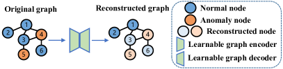
(a) Previous Reconstruction-based GAD Framework

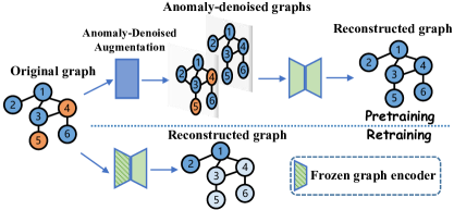
(b) The Proposed Two-stage GAD Framework

Figure 1: Workflow comparison. Previous reconstruction-based methods are trained on the contaminated graph. In contrast, our framework involves pretraining on anomaly-denoised graphs to reduce the impact of anomalous nodes.

The goal of unsupervised graph anomaly detection (GAD) is to identify rare patterns that deviate from the majority patterns in a graph, which has been extensively applied in diverse domains, such as fraud detection (Abdallah, Maarof, and Zainal 2016; Cheng et al. 2020; Dou et al. 2020) and social network (Fan, Zhang, and Li 2020; Duan et al. 2023). Recently, reconstruction-based Graph Neural Networks (GNNs) methods have achieved great success and have become the mainstream approach. The common assumption is that normal nodes are easier to be reconstructed than abnormal nodes. On this basis, such methods usually train a graph autoencoder and determine anomalies according to the magnitude of the reconstruction errors.

However, the anomalous patterns in the graph might hinder the performance of reconstruction-based methods in two ways. (1) Anomaly Overfitting: graphs in the real world are highly sparse, and powerful GNNs tend to overfit to anomalous features, leading to small reconstruction errors even for anomalies. This, in turn, can cause the model to fail. (2) Homophily Trap: Most GNNs operate under the homophily assumption (Kipf and Welling 2016a), which suggests that connected nodes share similar features. Therefore, the presence of anomalous nodes may hinder the reconstruction of nearby normal nodes, such that the corresponding magnified reconstruction errors bias the detection results. These phenomena are illustrated in Figure 1a. The reconstructed features of normal nodes 3 and 6 are influenced by their anomalous neighbors 4 and 5 due to Homophily Trap. Meanwhile, owing to Anomaly Overfitting, nodes 4 and 5 are well-reconstructed, far from what we expected.

We conduct a simple experiment to verify the negative effects of the anomalous patterns. Specifically, the popular DOMINANT baseline (Ding et al. 2019) are trained on the Cora and CiteSeer datasets (Sen et al. 2008) under three settings: on the original graph containing no abnormal nodes, on the partially-contaminated graph with $n/2$ injected anomalies, and on the graph with fully-injected $n$ anomalies. During the testing phase, all the models are tested on graphs with $n$ anomalies. As shown in Figure 2, the model trained on the clean graph consistently outperforms the others under different numbers of injected anomalies. Moreover, even converting only half of the anomalies into clean data for training can improve performance. Namely, the less the training data is contaminated, the better the detection performance is.

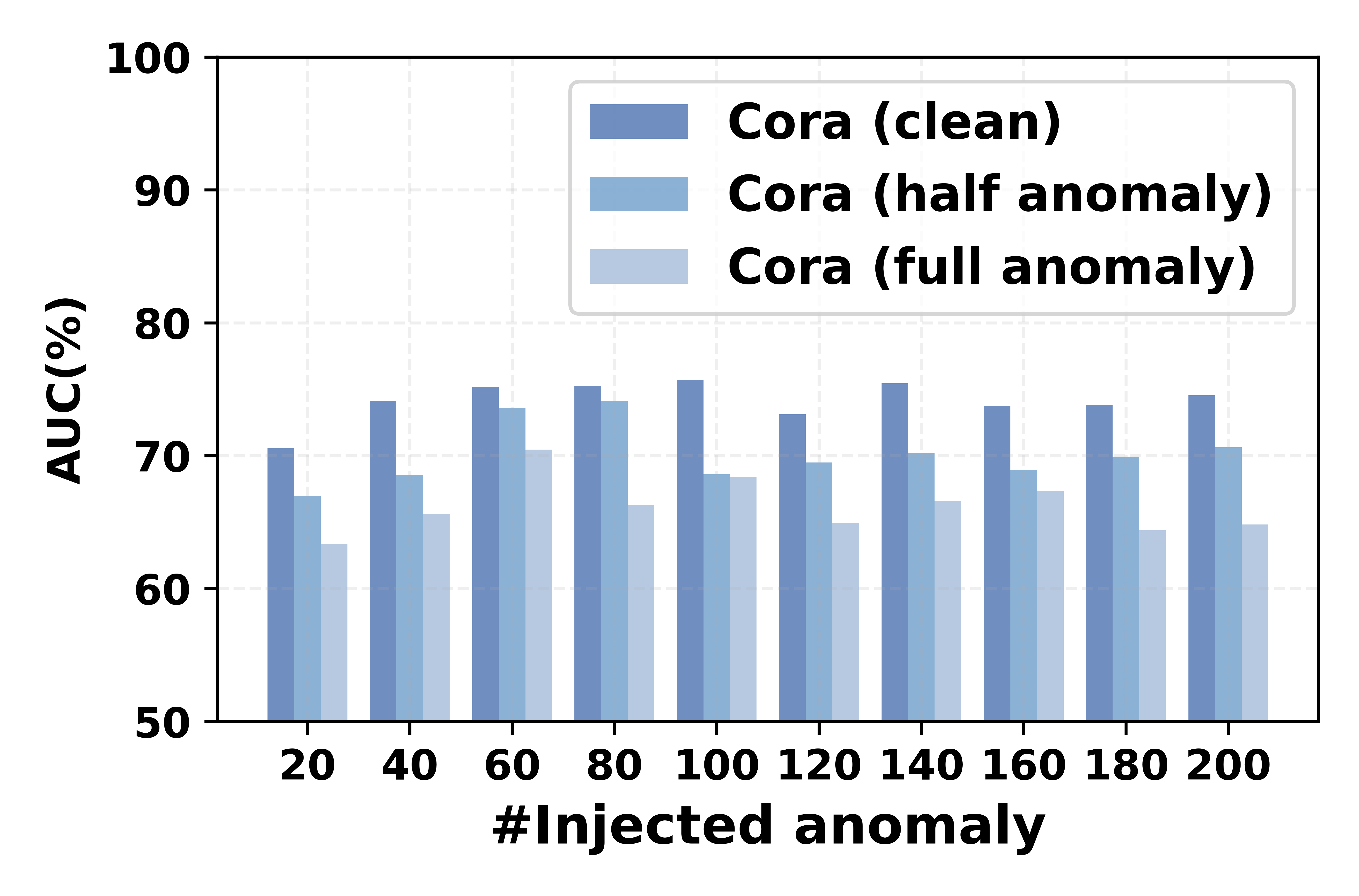
(a)

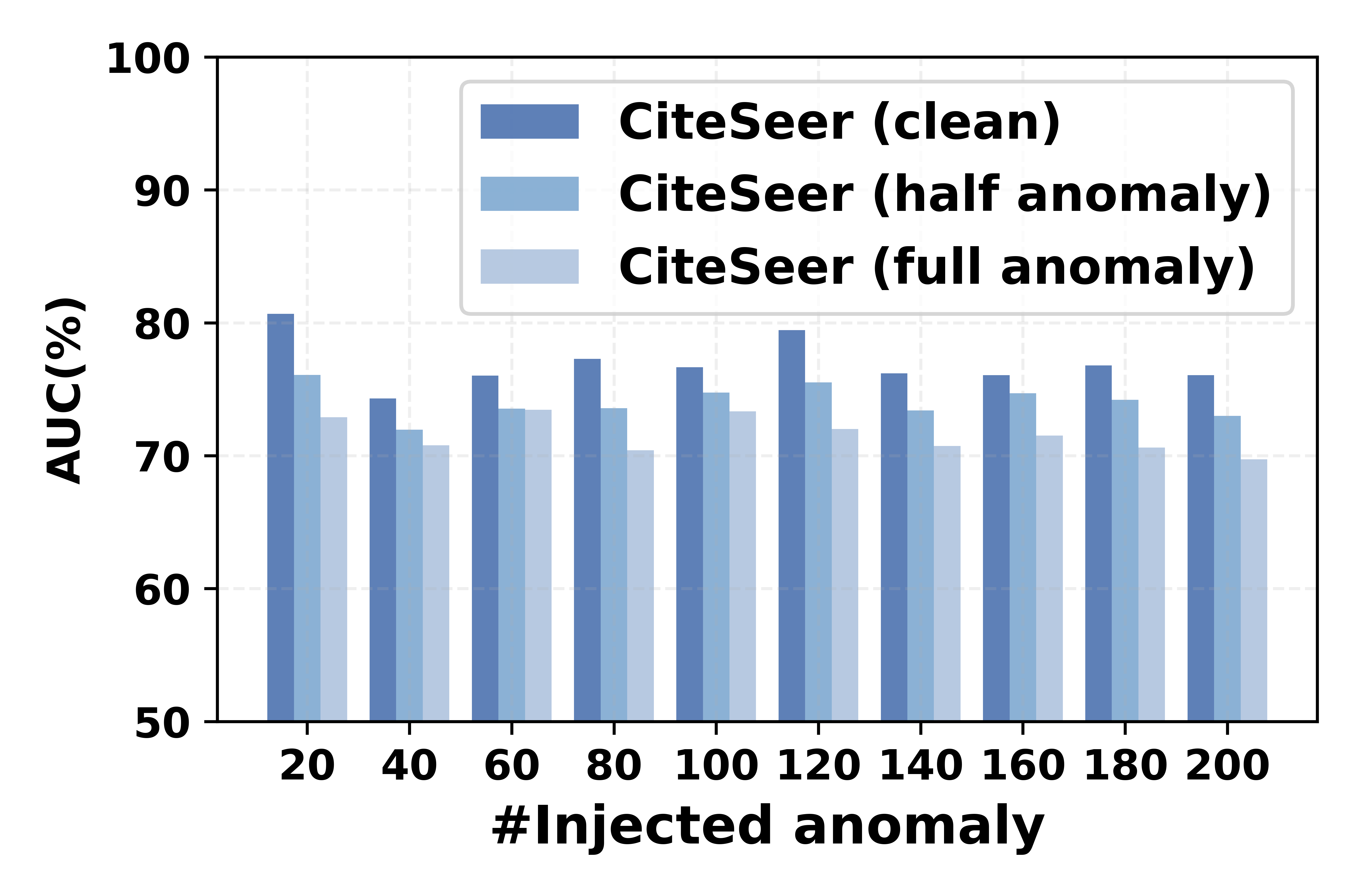
(b)

Figure 2: Detection performance of the DOMINANT model on Cora and CiteSeer datasets. The x-axis denotes the number of injected anomalies ($n$), while the y-axis shows the test results for models trained on graphs with clean (no anomalies), half-injected ($n/2$), or fully-injected ($n$) anomalies, but all evaluated on graphs containing $n$ injected anomalies. We see that the less the training data is contaminated, the better the performance is.

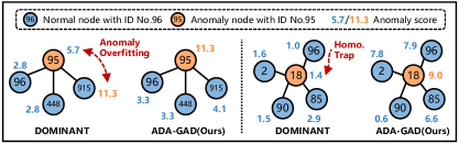
Figure 3: Real cases of Anomaly Overfitting and Homophily Trap on Disney and Books datasets. Compared with DOMINANT, our ADA-GAD can effectively mitigate these issues.

Motivated by this, we hope to train the model on a graph as clean as possible. Since the ground-truth clean graph is not available, we need to find a way to reduce the anomaly level of the graph for training and effectively leverage the graph for detection. To this aim, we present a two-stage framework called Anomaly-Denoised Autoencoders for Graph Anomaly Detection (ADA-GAD), as illustrated in Figure 1(b). (1) Stage 1: We develop a learning-free augmentation method to obtain cleaner graphs, whose anomaly degree is quantified by a spectral property-based metric. Such anomaly-denoised augmentation technique generates three levels of augmented graphs by masking: node-level, edge-level, and subgraph-level. Corresponding anomaly-denoised autoencoders are pretrained on these augmented graphs using masking pretraining strategies, forcing the model to discover normal patterns. (2) Stage 2: We freeze the pretrained encoders and retrain the decoders from scratch to reconstruct the original graph for detection. We utilize an attention mechanism to aggregate the frozen multi-level representations, and introduce node anomaly distribution regularization, which sharpens the anomaly score distribution of nodes to prevent Anomaly Overfitting. Subsequently, we identify anomalous nodes based on the magnitude of the reconstruction error. The efficacy of our ADA-GAD framework is visualized in Figure 3. In comparison with the previous methods, our ADA-GAD exhibits a significant reduction in the issues of Anomaly Overfitting and Homophily Trap.

The contributions of this paper are three-fold:

• To alleviate the phenomena of Anomaly Overfitting and Homophily Trap, we propose a two-stage graph anomaly detection framework ADA-GAD that firstly reduces the anomaly level of the graph for pretraining and then retrains the decoder for detection.

• In the pretraining stage, we present a metric to quantify the degree of anomaly in a graph. Then an anomaly-denoised augmentation strategy is introduced to generate augmented graphs with lower anomaly degrees for multi-level masking pretraining.

• In the retraining stage, we design a regularization term to make the distribution of each node’s anomaly score sharper, especially to overcome the Anomaly Overfitting issue.

Extensive experiments on two synthetic and five real-world anomaly datasets demonstrate the superiority of the proposed method.

Related Work

Graph Neural Networks

Graph neural networks (GNNs) are widely used in various deep learning tasks, as they can process graph-structured data and learn both the structural and attributive information of graphs (Kipf and Welling 2016a; Veličković et al. 2017; Gupta, Matta, and Pant 2021), which have achieved remarkable results in tasks such as social networks, recommendation systems and bioinformatics (Zhou et al. 2020; Waikhom and Patgiri 2021). GNNs can be divided into two types: spectral-based and spatial-based (Zhu et al. 2021a). Spectral-based GNNs use spectral graph theory and rely on the Laplacian matrix of the graph, while spatial-based GNNs use the spatial information of the nodes and rely on message passing mechanisms (Kipf and Welling 2016a; Xu et al. 2018). Typical spectral-based models include ChebNet (Defferrard, Bresson, and Vandergheynst 2016) and GCN (Kipf and Welling 2016a), while classical spatial-based GNNs are GAT (Velickovic et al. 2017), GraphSAGE (Hamilton, Ying, and Leskovec 2017), GIN (Xu et al. 2018), and GraphSNN (Wijesinghe and Wang 2022).

Anomaly Detection on Static Attributed Graphs

Graph anomaly detection (Duan et al. 2023) aims to identify nodes that are different from most nodes. Some progress has been made in anomaly detection on static attributed graphs. non-deep learning methods (Li et al. 2017; Peng et al. 2018) proposed techniques for detecting anomalous nodes in graphs based on matrix decomposition using homophily assumption, which states that connected nodes have similar features. Moreover, the exploration of deep learning (Peng et al. 2018; Li et al. 2019; Bandyopadhyay et al. 2020) for graph anomaly detection is steadily increasing. DOMINANT (Ding et al. 2019) introduces GCN as a graph autoencoder to process both network structure and node attribute information. AnomalyDAE (Fan, Zhang, and Li 2020) uses GAT to encode network structure information. AEGIS (Ding et al. 2021) introduces an unsupervised inductive anomaly detection method that can be applied to new nodes. (Chen et al. 2020) proposed to use generative adversarial networks (GANs) (Goodfellow et al. 2019) to generate anomalous nodes to support anomaly detection, while (Liu et al. 2021; Xu et al. 2022; Huang et al. 2023) presented contrastive learning techniques for graph anomaly detection.

Graph Self-Supervised Learning

Graph self-supervised learning (GSSL) (Lee, Lee, and Park 2022) is an unsupervised approach that learns meaningful representations from graph data by constructing pretext tasks (Liu et al. 2022c). Three types of GSSL methods can be distinguished based on the different pretext tasks: contrastive, generative, and predictive. Contrastive methods generate multiple views for each graph instance and learn graph representations by contrasting the similarity and difference between different views (You et al. 2020; Sun et al. 2019; Zhu et al. 2021c; Zeng and Xie 2021). Generative methods employ autoencoders to reconstruct parts of the input graph (Zhu, Du, and Yan 2020; Manessi and Rozza 2021; He et al. 2022; Hou et al. 2022). Predictive methods (Wu et al. 2021; Jin et al. 2020; Peng et al. 2020) use statistical analysis or expert knowledge to generate pseudo-labels for graph data and then design some prediction-based proxy tasks based on these pseudo-labels to learn graph representation.

Problem Definition

The primary focus of this work is to address the task of GAD in attributed networks. Following previous studies (Ding et al. 2019; Liu et al. 2022b), we consider the unsupervised setting in this paper, i.e., learning without both node category labels and anomaly labels. An attributed network can be represented as $\mathcal{G}=(\mathcal{V},\mathcal{E},\bm{X})$, where $\mathcal{V}=\{v_{1},\dots,v_{n}\}$ is the set of $n$ nodes, $\mathcal{E}$ is the set of $m$ edges, and $\bm{X}\in\mathbb{R}^{n\times d}$ is the attribute matrix. The structural information could also be represented by a binary adjacency matrix $\bm{A}\in\mathbb{R}^{n\times n}$. Specifically, $\bm{A}_{ij}=1$ if there exists a connection between nodes $v_{i}$ and $v_{j}$, and $\bm{A}_{ij}=0$ if not. The graph Laplacian matrix $\bm{L}$ is defined as $\bm{D}-\bm{A}$, where $\bm{D}$ is the degree matrix.

Given this attributed network, the aim of GAD is to identify nodes that deviate significantly from the majority in terms of both structural and attribute features. We attempt to formulate an anomaly function (Liu et al. 2022b) that assigns an anomaly score to each node $v_{i}$. Nodes that exceed the predefined anomaly threshold $\lambda$ are classified as anomalous, while others are considered normal.

The anomalous nodes in the attributed graph can be categorized into two types (Ma et al. 2021):

• Structural anomalies refer to densely connected nodes or other connection patterns that deviate from the sparsely connected regular nodes.

• Contextual anomalies are nodes whose attributes exhibit significant differences compared to their neighboring nodes.

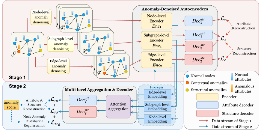
Figure 4: Overall framework of ADA-GAD. In Stage 1, we pretrain the graph autoencoders at three levels using the anomaly-denoised augmentation to mitigate the negative impact of anomalous patterns in the graph. In Stage 2, we retrain decoders based on multi-level embeddings obtained from fixed encoders, together with a regularization to sharpen the anomaly score’s distribution.

Methodology

Previous reconstruction-based GAD models usually consists of a graph encoder and two graph decoders. Specifically, the attribute decoder reconstructs the node attributes, and the structural decoder reconstructs the adjacency matrix. The resulting reconstruction errors from both decoders are combined to calculate anomaly scores for the nodes. These anomaly scores are then ranked, and nodes with higher scores are identified as anomalies.

As discussed in the Introduction, directly reconstructing the original graph containing mixed anomalies will suffer from Anomaly Overfitting and Homophily Trap, degenerating the detection performance. Ideally, training the graph autoencoders on the graph with fewer anomalies and utilizing it for detection is the best way to address this issue. However, this is infeasible in the unsupervised detection setting due to the absence of ground-truth anomaly information. Instead, we resort to an anomaly-denoised pretraining process which reduces the anomaly rate of the graph by augmentation and pretrains via the reconstruction on the anomaly-denoised graph. After mitigating the negative impact of anomalies on the encoder, we freeze it and only retrain the decoder on the original graph before proceeding with the subsequent detection. This forms a two-stage framework in Figure 4.

Stage 1: Anomaly-Denoised Pretraining

This stage generates the anomaly-denoised graphs and pretrains the graph autoencoders on them so that the auto-encoders can focus on the normal patterns. It paves the way for the subsequent anomaly detection stage by increasing the reconstruction error of anomalous nodes.

For the anomaly-denoised augmentation, we need to ensure that the anomaly level of the augmented graph is lower than that of the original graph. Then a key question arises: how to quantify the anomaly level of a graph? Some prior researches have shown that the level of anomaly in a signal $y$ on the graph $\mathcal{G}$ relates to its spectral statistics such as High-frequency Area Energy $E_{\text{high}}$ (Tang et al. 2022; Gao et al. 2023)

$$E_{\text{high}}(\mathcal{G},\bm{y})=\frac{\bm{y}^{T}\bm{L}\bm{y}}{\bm{y}^{T}\bm{y}}.$$ (1)

As the anomaly ratio of signal $y$ in the graph $\mathcal{G}$ increases, $E_{\text{high}}(\mathcal{G},\bm{y})$ also increases, known as ‘right-shift’ (Tang et al. 2022). Inspired by this, we define the anomaly degree at the attribute and structure level based on the corresponding characteristics as follows.

Definition 1 (Attribute Anomaly Magnitude)

The attribu-te anomaly magnitude on the graph $\mathcal{G}$ is defined as:

$$A_{\text{ano}}(\mathcal{G})=E_{\text{high}}(\mathcal{G},\bm{X})=\frac{\bm{X}^{T}\bm{L}\bm{X}}{\bm{X}^{T}\bm{X}}.$$ (2)

Definition 2 (Structural Anomaly Magnitude)

The structural anomaly magnitude on the graph $\mathcal{G}$ is defined as:

$$S_{\text{ano}}(\mathcal{G})=E_{\text{high}}(\mathcal{G},\bm{D})=\frac{\bm{D}^{T}\bm{L}\bm{D}}{\bm{D}^{T}\bm{D}}.$$ (3)

A larger $A_{\text{ano}}$ for $\mathcal{G}$ indicates more pronounced variations in its attributes, leading to a higher ratio of contextual anomalies. And $S_{\text{ano}}$ characterizes the ratio of structural anomalies similarly.

Definition 3 (Graph Anomaly Magnitude)

The anomaly magnitude on a graph $\mathcal{G}$ is defined as the sum of the attribute anomaly magnitude $A_{\text{ano}}$ and the structural anomaly magnitude $S_{\text{ano}}$:

$$G_{\text{ano}}(\mathcal{G})=A_{\text{ano}}(\mathcal{G})+S_{\text{ano}}(\mathcal{G}).$$

Apparently, as the proportion of anomalous nodes within the graph increases, the graph anomaly magnitude also tends to rise. This provides a good measure for the anomaly-denoised augmentation process. The objective of the augmentation is to minimize the anomaly level of the augmented graph $\mathcal{G}^{\prime}=(\bm{X}^{\prime},\bm{A}^{\prime})$ within predefined augmentation budgets:

$$\underset{\begin{subarray}{c}\bm{A}^{\prime},\bm{X}^{\prime}\end{subarray}}{\text{minimize}}\quad G_{\text{ano}}(\mathcal{G}^{\prime}),$$ (4)

subject to $$\alpha\leq G_{\text{ano}}(\mathcal{G})-G_{\text{ano}}(\mathcal{G}^{\prime})\leq\beta,$$

$$\begin{aligned} \|\bm{X}-\bm{X}^{\prime}\|^{2}_{F}\leq\epsilon_{1},\|\bm{A}-\bm{A}^{\prime}\|^{2}_{F}\leq\epsilon_{2},\end{aligned}$$

where $\alpha>0$ and $\beta>0$ set the acceptable bounds for anomaly rate reduction, $\|\cdot\|_{F}$ denotes the Frobenius norm. Additionally, $\epsilon_{1}$ and $\epsilon_{2}$ are both small and denote the augmentation budget for the attribute and structure, respectively.

However, because the graph’s adjacency matrix is discrete, directly solving this optimization problem is very challenging (Zhu et al. 2021b). Thus, we turn to design a learning-free augmentation approach to achieve our goal. We introduce a simplified graph masking strategy to generate the augmented graph and conduct denoising pretraining at three levels: node-level, edge-level, and subgraph-level.

Node-level denoising pretraining

For node-level anomaly denoising, we randomly select a subset of nodes $\mathcal{V}^{n}\subset\mathcal{V}$ for replacement-based masking using a probability of $p_{r}$. The masked node features are adjusted as follows:

$$\widetilde{\bm{x}}_{i}=\begin{cases}\bm{x}_{j}&v_{i}\in\mathcal{V}^{n}\\ \bm{x}_{i}&v_{i}\notin\mathcal{V}^{n},\end{cases}$$ (5)

where we randomly choose another node (denoted as $j$) and replace the original feature $\bm{x}_{i}$ with $\bm{x}_{j}$ if $v_{i}\in\mathcal{V}^{n}$. Additionally, we also introduce a probabilistic mechanism where the feature of each node $v_{i}\in\mathcal{V}^{n}$ is randomly transited to zero with a probability of $p_{z}$. After the augmentation, we could calculate the corresponding graph anomaly magnitude and check if it satisfies the constraint in Problem (4). The augmented graph is valid if the condition holds.

We repeat the above augmentation steps multiple times, generating a collection of valid augmented graphs of length $l_{n}$, denoted as $\mathcal{C}_{n}=\{\mathcal{G}_{1}^{n},\mathcal{G}_{2}^{n},...,\mathcal{G}_{l_{n}}^{n}\}$, where each $\mathcal{G}_{k}^{n}=(\mathcal{V},\mathcal{E},\bm{X}_{k}^{n})$ satisfies $G_{\text{ano}}(\mathcal{G}_{k}^{n})\leq\theta$, $\bm{X}_{k}^{n}$ is the masked attribute matrix generated each time, $\theta=G_{\text{ano}}(\mathcal{G})-\alpha$ is the anomaly degree threshold.

For each $\mathcal{G}_{k}^{n}$, we feed it into the node-level graph autoencoders consisting of the GNN encoder $Enc_{1}$ and the attribute decoder $Dec_{1}^{att}$ (Ding et al. 2019; Fan, Zhang, and Li 2020), and then obtain the reconstructed features:

$$\bm{\hat{\bm{X}}}_{k}^{n}=Dec_{1}^{att}(Enc_{1}(\mathcal{G}^{n}_{k})).$$ (6)

In the pretraining, the autoencoder should especially learn to reconstruct the feature $\bm{x}_{i}$ of the masked node $v_{i}\in\mathcal{V}$. Then the node-level reconstruction loss $\mathcal{L}_{n}$ is the sum of reconstruction losses over $\mathcal{C}_{n}$:

$$\mathcal{L}_{n}=\sum^{l_{n}}_{k=1}\|\bm{X}_{k}^{n}-\hat{\bm{X}}_{k}^{n}\|_{F}^{2}.$$ (7)

Edge-level denoising pretraining

Similar to the node-level pretraining, we randomly select a subset of edges $\mathcal{E}^{e}$ from $\mathcal{E}$ and apply masking with a probability of $q$, resulting in the corresponding entries in the adjacency matrix being set to zero. After multiple times of augmentation, we obtain a collection of $l_{e}$ edge masking graphs, denoted as $\mathcal{C}_{e}=\{\mathcal{G}_{1}^{e},\mathcal{G}_{2}^{e},...,\mathcal{G}_{l_{e}}^{e}\}$, where each $\mathcal{G}_{k}^{e}=(\mathcal{V},\mathcal{E}\setminus\mathcal{E}^{e}_{k},\bm{X})$ also fulfills the condition $G_{\text{ano}}(\mathcal{G}_{k}^{e})\leq\theta$, $\mathcal{E}^{e}_{k}$ is edge subset generated each time.

The edge-level autoencoders take the edge-level masked graph $\mathcal{G}_{k}^{e}$ as input and aim to reconstruct the denoised graph structure $\mathcal{E}\setminus\mathcal{E}^{e}_{k}$. The reconstructed adjacency matrix for each augmented $\bm{A}_{k}^{e}$ can be expressed as:

$$\bm{\hat{\bm{A}}}_{k}^{e}=Dec_{2}^{str}(Enc_{2}(\mathcal{G}^{e}_{k})),$$ (8)

where $Enc_{2}$ and $Dec_{2}^{str}$ denote the GNN encoder and the structural decoder, respectively.

The loss function of the edge-level autoencoders $\mathcal{L}_{\text{e}}$ can be defined as:

$$\mathcal{L}_{e}=\sum^{l_{e}}_{k=1}\|\bm{A}_{k}^{e}-\hat{\bm{A}}_{k}^{e}\|_{F}^{2}.$$ (9)

Subgraph-level denosing pretraining

In addition, we propose a novel pretext task of subgraph masking pretraining. We employ random walk-based subgraph sampling for masking, adopting similar node and edge masking strategies as the above masking processes. In the resulted augmented graph sets $\mathcal{C}_{s}=\{\mathcal{G}_{1}^{s},\mathcal{G}_{2}^{s},...,\mathcal{G}_{l_{s}}^{s}\}$, each $\mathcal{G}_{k}^{s}=(\mathcal{V},\mathcal{E}\setminus\mathcal{E}^{s}_{k},\bm{X}_{k}^{s})$ satisfies $G_{\text{ano}}(\mathcal{G}_{k}^{s})\leq\theta$, where $\mathcal{E}^{s}_{k}$ is edge subset generated each time, $\bm{X}_{k}^{s}$ is attribute matrix generated each time.

Subgraph-level masking can be viewed as a specific combination of node- and edge-level masking. The reconstructed feature and structure are:

$$\hat{\bm{A}}^{s}_{k} =Dec_{3}^{att}(Enc_{3}(\mathcal{G}_{k}^{s})),$$ (10)

$$\bm{\hat{X}}^{s}_{k} =Dec_{3}^{str}(Enc_{3}(\mathcal{G}_{k}^{s})),$$

where $Enc_{3}$ is a GNN encoder, $Dec_{3}^{att}$ and $Dec_{3}^{str}$ denote the attribute and structure decoder, respectively. The corresponding reconstruction loss function can be formulated as follows:

$$\mathcal{L}_{s}=\mathcal{L}_{sn}+\mathcal{L}_{se},$$ (11)

where $\mathcal{L}_{sn}$ and $\mathcal{L}_{se}$ are computed by substituting $\bm{\hat{X}}^{s}_{k}$ and $\hat{\bm{A}}^{s}_{k}$ into Eq. (7) and (9), respectively.

In Stage 1, all the above three procedures are simultaneously adopted to pretrain the corresponding autoencoders. The various levels of denoising pretraining help the model discover the underlying normal node patterns.

Stage 2: Retraining for Detection

In this stage, the graph is no longer masked for learning. We fix the pretrained graph encoders, discard the pretrained decoders and retrain two unified decoders (one for attribute and another for structure) from scratch to detect anomalous information in the graph.

Multi-level embedding aggregation

The pretrained encoders produce embeddings at three levels. They are firstly passed through a fully connected layer, and then aggregated using an attention mechanism. This yields an aggregated multi-level embedding denoted as $\bm{h}$ for each node.

Graph reconstruction for anomaly detection

The aggregated multi-level embeddings $\bm{h}$ are fed into an attribute decoder $Dec^{att}_{f}$ and a structure decoder $Dec_{f}^{str}$ for reconstruction. Specifically, we reconstruct the adjacency matrix $\bm{A}$ and attribute matrix $\bm{X}$ of the original graph as $\hat{\bm{A}}$ and $\hat{\bm{X}}$, respectively. The corresponding graph reconstruction loss $\mathcal{L}_{rec}$ is:

$$\mathcal{L}_{rec} =(1-\gamma)\mathcal{L}_{rs}+\gamma\mathcal{L}_{ra}$$ (12)

$$=(1-\gamma)\|\bm{A}-\hat{\bm{A}}\|_{F}^{2}+\gamma\|\bm{X}-\hat{\bm{X}}\|_{F}^{2},$$

where $\gamma\in[0,1]$ is a balance hyperparameter. And the anomaly score $s_{i}$ for the $i$-th node is defined as:

$$s_{i}=(1-\gamma)\left\|\bm{a}_{i}-\hat{\bm{a}}_{i}\right\|_{2}+\gamma\left\|\bm{x}_{i}-\hat{\bm{x}}_{i}\right\|_{2}.$$ (13)

where $\hat{\bm{a}}_{i}$ and $\bm{a}_{i}$ represent the reconstructed and original structure vector of node $v_{i}$, respectively. Similarly, $\hat{\bm{x}}_{i}$ and $\bm{x}_{i}$ are the $i$-th reconstructed and original attribute vector, respectively.

Node Anomaly Distribution Regularization

We propose a novel approach to regularize the model with a node anomaly distribution loss $\mathcal{L}_{s}$ that enforces sparsity on the anomaly distribution, further mitigating the Anomaly Overfitting. Considering that overfitting occurs when all nodes are reconstructed very well, we intentionally introduce some non-uniformity in the anomaly distribution around nodes to enhance the difficulty of reconstruction. Therefore, we require the following anomaly distribution $\mathcal{A}_{i}$ of node $v_{i}$, e.g., the anomaly scores of a node and its neighbors, to be sharper:

$$\mathcal{A}_{i}=\frac{s_{i}^{-\tau}}{\sum_{j\in\mathcal{N}_{i}}s_{j}^{-\tau}},$$ (14)

where $\mathcal{N}_{i}$ represents the neighborhood of node $v_{i}$, and $\tau\in(0,1)$ is a temperature coefficient. Then the corresponding entropy $\mathcal{S}_{i}$ is:

$$\mathcal{S}_{i} =-\mathcal{A}_{i}\log\mathcal{A}_{i}$$ (15)

$$=\frac{s_{i}^{-\tau}}{\sum_{j\in\mathcal{N}_{i}}s_{j}^{-\tau}}(\log\sum_{j\in\mathcal{N}_{i}}s_{j}^{-\tau}-\tau\log s_{i}).$$

In fact, $\mathcal{S}_{i}$ represents the smoothness level of the anomaly distribution around node $i$. A higher value of $\mathcal{S}_{i}$ indicates a sharper anomaly distribution. Accordingly, the node anomaly distribution regularization term $\mathcal{L}_{reg}$ is defined as:

$$\mathcal{L}_{reg}=-\sum_{v_{i}\in\mathcal{V}}\mathcal{S}_{i}.$$ (16)

Optimization Objective

Putting all together, we have the overall loss function in this stage:

$$\mathcal{L} =\mathcal{L}_{rec}+\mathcal{L}_{reg}$$ (17)

$$=(1-\gamma)\mathcal{L}_{ra}+\gamma\mathcal{L}_{rs}+\gamma_{reg}\mathcal{L}_{reg},$$

where $\gamma_{reg}$ is a weight hyperparameter that should be small to avoid influencing optimization of $\mathcal{L}_{rec}$. Based on this loss, we retrain the aggregation and the decoder modules. After retraining, we sort the nodes based on their anomaly scores $s_{i}$, and take the nodes with higher $s_{i}$ as anomalous nodes according to the given anomaly rate.

Experiments

Experimental Setup

Datasets

Table 1: Statistics of dataset ($*$ indicates the dataset with injected anomalies).

Dataset	Nodes	Edges	Feat	Anomalies	Ratio
Cora∗	2,708	11,060	1,433	138	5.1%
Amazon∗	13,752	515,042	767	694	5.0%
Weibo	8,405	407,963	400	868	10.3%
Reddit	10,984	168,016	64	366	3.3%
Disney	124	335	28	6	4.8%
Books	1,418	3,695	21	28	2.0%
Enron	13,533	176,987	18	5	0.4%

We conducted experiments on two datasets injected with synthetic anomalies: Cora (Sen et al. 2008), Amazon (Shchur et al. 2018), and five manually labeled datasets with anomalies: Weibo (Zhao et al. 2020), Reddit (Kumar, Zhang, and Leskovec 2019), Disney (Müller et al. 2013), Books (Sánchez et al. 2013), and Enron (Sánchez et al. 2013). We injected contextual anomalies into datasets with no labeled anomalies by swapping node attributes, and structural anomalies by altering node connections within the graph, maintaining an equal number for each type in alignment with prior research (Ding et al. 2019; Liu et al. 2022a). The statistics of all the datasets are recorded in Table 1.

Table 2: AUC (%) results (mean $\pm$ std). The best result is shown in bold, while the second best is marked with underline.

Algorithm		Cora	Amazon	Weibo	Reddit	Disney	Books	Enron
	SCAN	64.95±0.00	65.85±0.00	70.63±0.00	49.67±0.00	50.85±0.00	52.42±0.00	53.70±0.00
	Radar	53.28±0.00	58.93±0.00	98.27±0.00	56.64±0.00	50.14±0.00	56.21±0.00	64.10±0.00
Non-Deep	ANOMALOUS	35.13±1.07	71.49±1.71	98.27±0.00	51.58±8.66	50.14±0.00	52.51±0.00	63.65±0.36
	MLPAE	70.91±0.07	74.20±0.00	90.01±0.42	49.74±1.70	48.02±0.00	51.28±5.36	41.55±2.59
	GCNAE	70.90±0.00	74.20±0.00	88.98±0.31	50.70±0.46	47.34±1.31	54.81±1.59	66.86±0.54
	DOMINANT	76.71±0.07	74.20±0.00	92.17±0.41	56.20±0.06	52.91±3.04	40.14±2.66	54.93±0.66
	DONE	83.60±1.45	73.38±4.37	86.86±0.38	51.40±2.26	48.42±4.23	54.05±1.64	61.07±3.15
	AdONE	82.12±0.71	79.31±2.60	82.98±0.63	51.53±1.38	50.93±2.34	54.13±1.60	58.36±7.34
	AnomalyDAE	80.99±0.07	77.39±0.01	92.99±0.44	52.21±2.03	48.29±4.17	59.86±4.82	45.85±13.16
	GAAN	68.32±1.38	77.70±0.34	92.53±0.01	51.23±1.19	48.02±0.00	53.38±2.13	56.55±11.69
	CoLA	56.88±1.63	61.00±1.09	22.18±3.36	53.21±1.10	54.46±7.67	49.69±4.20	58.53±9.38
	OCGNN	50.02±0.14	49.99±0.04	79.68±5.76	48.76±3.57	68.19±1.45	57.33±4.14	54.39±6.11
	CONAD	84.34±0.03	82.62±0.26	90.87±0.59	56.02±0.01	45.38±4.64	40.82±1.18	54.67±0.48
	ADA-GADrand	81.61±0.01	76.36±0.12	90.74±0.65	56.03±0.38	68.56±2.94	61.75±2.20	66.12±4.87
	ADA-GADnode	84.13±0.02	77.38±0.02	96.39±0.74	56.33±0.16	68.05±3.70	62.77±2.31	71.55±2.27
	ADA-GADedge	84.10±0.01	81.85±0.03	94.52±0.70	56.37±0.10	68.42±3.19	62.71±2.17	72.34±1.42
	ADA-GADsubgraph	84.42±0.01	81.79±0.04	96.69±0.59	55.58±0.36	68.59±2.62	62.70±2.13	72.86±0.88
Deep	ADA-GAD	84.73±0.01	83.25±0.03	98.44±0.33	56.89±0.01	70.04±3.08	65.24±3.17	72.89±0.86

Competitors

We adopt three non-deep learning methods for graph anomaly detection comparison: SCAN (Xu et al. 2007), Radar (Li et al. 2017), ANOMALOUS (Peng et al. 2018). Additionally, we have also selected the following deep learning-based competitors: GCNAE (Kipf and Welling 2016b), DOMINANT (Ding et al. 2019), DONE (Bandyopadhyay et al. 2020), AdONE (Bandyopadhyay et al. 2020), AnomalyDAE (Sakurada and Yairi 2015), GAAN (Chen et al. 2020), CoLA (Liu et al. 2021), OCGNN (Wang et al. 2021), CONAD (Xu et al. 2022).

Meanwhile, we also implement four variants of the proposed ADA-GAD method to verify the effectiveness of the anomaly-denoised augmentation: ADA-GAD_rand refers to using random augmentation; ADA-GAD_node, ADA-GAD_edge, and ADA-GAD_subgraph utilize a single level of anomaly-denoised augmentation, denoising pretrained at only the node, edge, and subgraph level, respectively.

Implementation Details

We implement all the competitors with the PyGOD toolbox (Liu et al. 2022a). We set the number of epochs/dropout rate/weight decay to 100/0.1/0.01, respectively. The embedding dimension $d$ is set to 12 for the Disney, Books, and Enron datasets, and 64 for the others.

Our ADA-GAD method utilizes GCN as the encoders and decoders, except for the Enron and Weibo datasets, where we adopt GAT as the encoders and GCN as decoders. For the real-world datasets Disney, Books, and Enron, the encoder depth is set to 2 and the decoder depth is 1. For the other datasets, encoder and decoder depths are set to 1. During augmentation, the number of masks for nodes and edges is set within the range of 1 to 20, respectively. The number of random walks and walk length for the subgraph mask are both set to 2. $l_{n}$, $l_{e}$, and $l_{s}$ are all set to 10, with $\theta$ is assigned to the smallest $G_{\text{ano}}$ among $N\_{aug}$ random augmentations. In the experiments, $N\_{aug}$ is set to 30. The pre-training epoch and the retain epoch are both set to 20. AUC (Area under the ROC Curve) (Bradley 1997) is used as the performance metric. We repeat all experiments 10 times using 10 different seeds.

Performance Comparison

All the experimental results are reported in Table 2 reports all the experimental results. From the results, we have the following observations: (1) ADA-GAD consistently exhibits better AUC performance than other competitors, which validates the effectiveness of the proposed method. (2) A single anomaly-denoised pretraining branch is a little inferior to the combination of three-level anomaly-denoised pretraining branches but outperforms the random one. This phenomenon indicates that our anomaly-denoised training strategy successfully utilizes the information at the node, edge, and subgraph levels for anomaly detection. (3) On four datasets with relatively small feature dimensions (i.e., Reddit, Disney, Books, and Enron), some competitors might achieve poor AUC performances, which is consistent with the empirical results in the benchmark (Liu et al. 2022b). In contrast, our ADA-GAD demonstrates consistent improvement over the competitors, which again validates our motivation. (4) The non-deep learning methods, Radar and ANOMALOUS, outperform the other deep learning competitors on the Weibo and Reddit datasets. This counter-intuitive result indicates that these deep learning methods might suffer from severe over-fitting. As a comparison, the proposed method utilizes the denoised augmentation of real-world datasets and takes anomaly-denoised graphs as inputs, which forces the model to pay more attention to normal patterns during pretraining and thus overcomes the over-fitting issue.

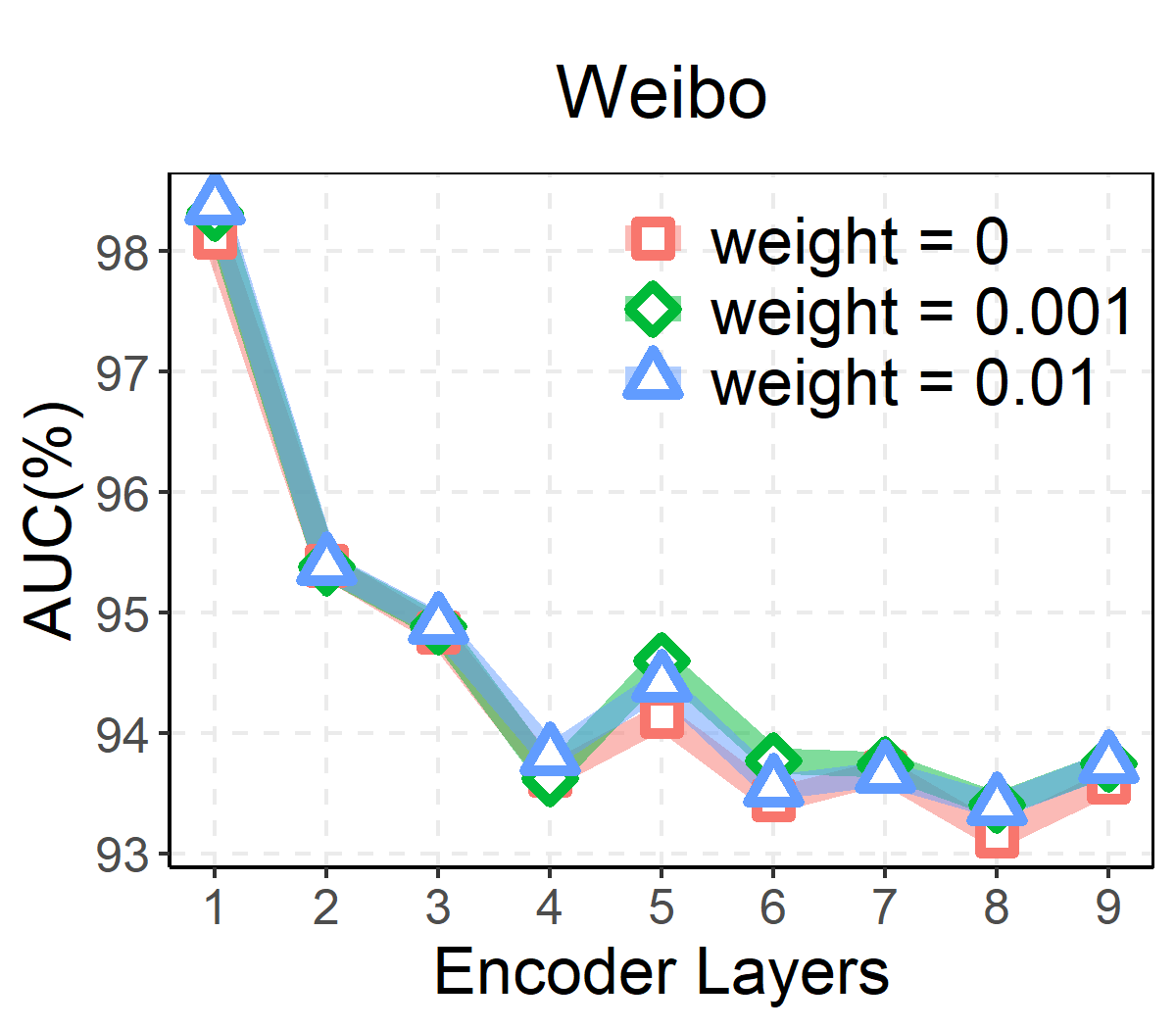
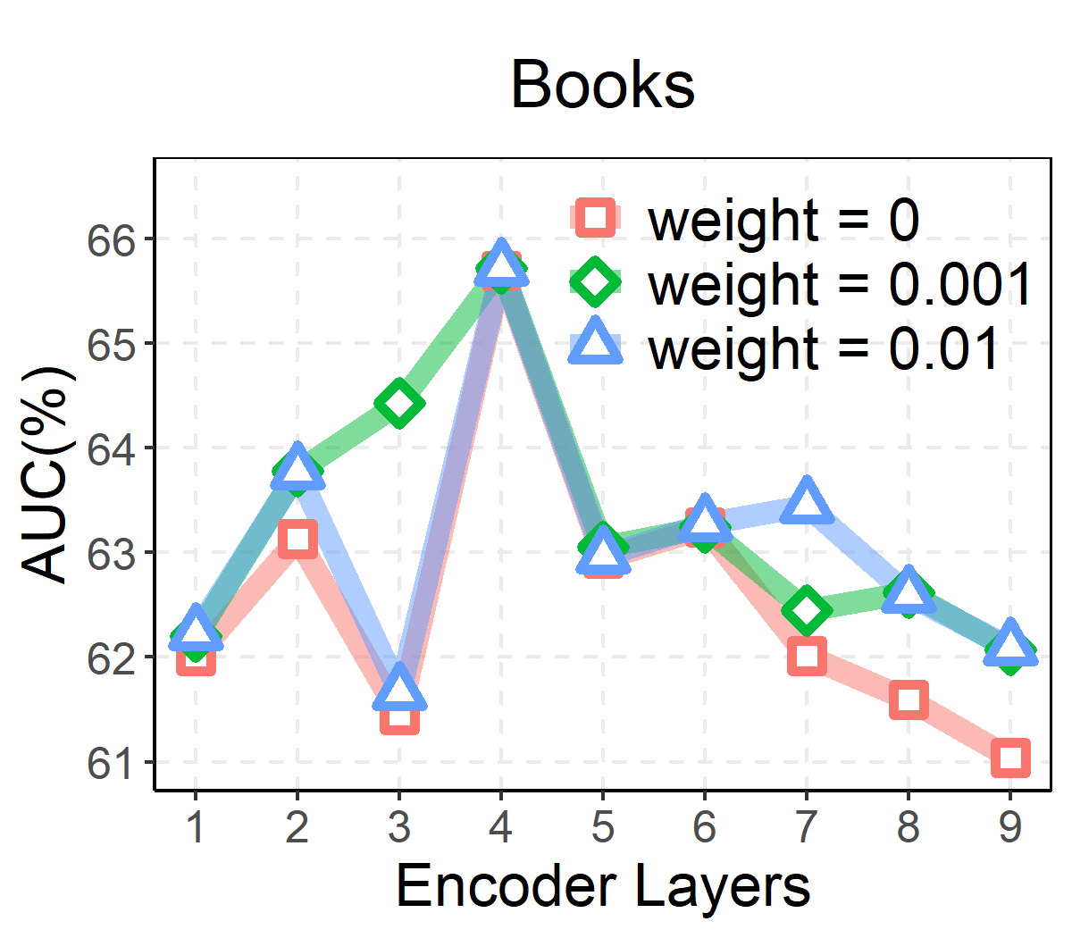
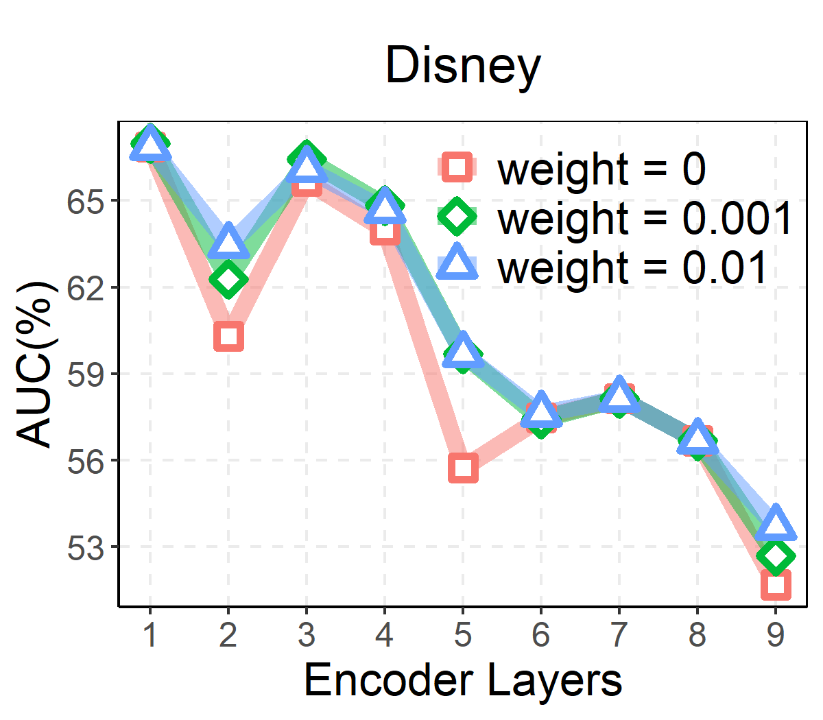
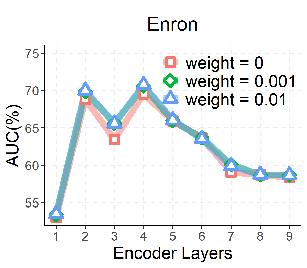
Figure 5: Effect of the encoder depth and weight of node anomaly distribution regularization on four organic datasets.

Ablation Study

Studies on Aggregation Strategies

We explored different aggregation strategies: non-learnable linear, learnable linear, and our attention aggregation. The non-learnable method uses fixed weights, whereas the learnable method optimizes weights through gradient descent. Figure 6 demonstrates the superior performance of our attention aggregation, highlighting its enhanced efficacy.

Studies on the Model Depth and Node Anomaly Distribution Regularization

To investigate the effectiveness of our model at different network depths, we evaluate the performance of the encoder with the number of layers ranging from 1 to 9 under different weights (0, 0.01, 0.001) of the node anomaly distribution regularization. As shown in Figure 5, we can find that (1) the optimal number of encoder layers varies across datasets, with the Weibo dataset having an optimal number of 1 and the other three real-world datasets having an optimal number of 3 or 4. This suggests that the Weibo dataset is more prone to overfitting, consistent with our previous experimental findings. (2) After reaching the optimal number of layers, increasing the depth fails to improve performance. Fortunately, the node anomaly distribution regularization can alleviate this issue, as a larger weight within a small range can induce better performance.

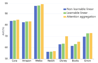
Figure 6: Performance comparison using different aggregation strategies.

Conclusion

In this paper, we introduced ADA-GAD, a novel two-stage framework for graph anomaly detection. Through anomaly-denoised augmentation and a two-stage training framework, ADA-GAD effectively captures the normal patterns and enhances anomaly detection performance. Additionally, we introduce a node anomaly distribution regularization term to mitigate the model overfitting by constraining the anomaly distribution near nodes. Experimental results demonstrate that our proposed method achieves state-of-the-art performance on multiple benchmarks with injected or organic anomalous nodes. Future research can explore further refinements and extensions of ADA-GAD in different types of anomaly detection scenarios, such as supervised settings or graph-level anomaly detection.

Appendix

Signals in Graphs

Given a graph $\mathcal{G}=(\mathcal{V},\mathcal{E},\bm{X})$, where $\mathcal{V}$ represents the set of vertices, $\mathcal{E}$ represents the set of edges, and $\bm{X}$ represents the node features, the normalized Laplacian matrix $\bm{L}$ is defined as $\bm{D}-\bm{A}$, where $\bm{A}$ is the adjacency matrix and $\bm{D}$ is the degree matrix with $\bm{D}_{ii}=\sum_{j}\bm{A}_{ij}$.

By performing the eigendecomposition on the Laplacian matrix $\bm{L}$, we obtain the eigenvalues arranged in ascending order as $0=\lambda_{1}\leq\lambda_{2}\leq\cdots\leq\lambda_{n}$ and their corresponding eigenvectors $\bm{U}=(\bm{u}_{1},\bm{u}_{2},\cdots,\bm{u}_{n})$. This decomposition provides valuable insights into the graph’s structural properties and spectral characteristics, forming the basis for various graph analysis and processing techniques.

We represent the signal on the graph $\mathcal{G}$ as $\bm{y}=(y_{1},y_{2},\cdots,y_{n})^{T}\in\mathbb{R}^{n}$. Using the eigenvectors $\bm{U}$ of the Laplacian matrix as the basis functions for the graph Fourier transform, we obtain $\bm{\hat{y}}=\bm{U}^{T}\bm{y}=(\hat{y}_{1},\hat{y}_{2},\cdots,\hat{y}_{N})^{T}$. Signals associated with high-frequency eigenvalues are referred to as high-frequency signals, whereas signals associated with low-frequency eigenvalues are considered as low-frequency signals on the graph.

High-frequency Area Energy

Based on previous studies (Tang et al. 2022; Gao et al. 2023), the spectral energy $S_{ene}$ at $\lambda_{k}$ ($1\leq k\leq N$) is given by:

$$S_{ene}(\mathcal{G},k)=\hat{y}_{k}^{2}/\sum_{i=1}^{N}\hat{y}_{i}^{2}.$$ (18)

The high-frequency area energy $E_{\text{high}}$ concerning the signal $\bm{y}$ on graph $\mathcal{G}$ can be calculated as follows:

$$E_{\text{high}}(\mathcal{G},\bm{y})=\frac{\sum_{k=1}^{N}\lambda_{k}\hat{y}^{2}_{k}}{\sum_{k=1}^{N}\hat{y}_{k}^{2}}=\frac{\bm{y}^{T}\bm{L}\bm{y}}{\bm{y}^{T}\bm{y}}.$$ (19)

As the spectral energy of high-frequency signals $S_{ene}$ becomes concentrated in the larger eigenvalues, there is a corresponding increase within the high-frequency area energy $E_{\text{high}}$. Furthermore, due to the correlation between higher-frequency signals in the graph and fewer distinct patterns, an increase in the anomaly rate of signal $\bm{y}$ within the graph results in a corresponding energy increase in the high-frequency area $E_{\text{high}}(\mathcal{G},\bm{y})$. For detailed explanation and proof, please refer to (Tang et al. 2022).

Datasets Details

Datasets

We conducted experiments on three datasets without manual labeling of anomalies:

• Cora (Sen et al. 2008) is a collection of 2,708 computer science papers categorized into seven classes, with attributes such as titles, abstracts, and keywords used for node classification and graph neural network algorithm evaluation.

• Amazon (Shchur et al. 2018) is a product classification dataset extracted from the Amazon marketplace.

Following the approach of previous studies (Ding et al. 2019; Liu et al. 2022a; Fan, Zhang, and Li 2020), we inject synthetic anomalous nodes into the Cora and Amazon datasets. Specifically, attribute anomalies are obtained by swapping some node attributes in the graph, while structural anomalies are obtained by changing some node connections.

Besides, we also conduct experiments on five manually labeled datasets (also known as organic datasets or real-world datasets (Liu et al. 2022b)) with anomalies:

• Weibo (Zhao et al. 2020) is a user-post-tag graph dataset from Tencent-Weibo, with suspicious users labeled based on temporal behavior.

• Reddit (Kumar, Zhang, and Leskovec 2019) is a user-subreddit graph dataset from the platform Reddit, with banned users labeled as anomalies.

• Disney (Müller et al. 2013) and Books (Sánchez et al. 2013) are co-purchasing networks of movies and books from Amazon, with anomalies labeled by high school students (Disney) or extracted from amazon information (Books).

• Enron (Sánchez et al. 2013) is an email network dataset with anomalies labeled based on identifying spam-sending email addresses.

Competitors Details

Non-deep learning methods

We adopt three for graph anomaly detection comparison:

• SCAN (Xu et al. 2007) detects clusters, hub nodes, and structural outliers in a graph by analyzing its structure.

• Radar (Li et al. 2017) detects outlier nodes by characterizing the residuals of attribute information and its coherence with network information.

• ANOMALOUS (Peng et al. 2018) performs joint anomaly detection and attribute selection to detect node anomalies based on the CUR decomposition and residual analysis, using both graph structure and node attribute information.

Deep learning methods

We also adopt the following deep learning-based anomaly detection methods as competitors:

• MLPAE (Sakurada and Yairi 2014) employs a multiple layer perceptron (MLP) (Gardner and Dorling 1998) as both an encoder and a decoder, utilizing a reconstruction-based approach for detecting and reconstructing node attributes.

• GCNAE (Kipf and Welling 2016b) uses GCNs as both encoder and decoder to learn node embeddings and reconstruct node attributes.

• DOMINANT (Ding et al. 2019) combines GCN and Autoencoders (AE) (Bank, Koenigstein, and Giryes 2020) for outlier node detection by using two-layer GCN as encoder, two-layer GCN as decoder for attribute reconstruction, and one-layer GCN and dot product as a structural decoder.

• DONE (Bandyopadhyay et al. 2020) leverages structural and attribute AE with MLP for adjacency matrix and node attribute reconstruction.

• AdONE (Bandyopadhyay et al. 2020) is a variant of DONE that uses an extra discriminator for better alignment of embeddings.

• AnomalyDAE (Fan, Zhang, and Li 2020) utilizes structure AE and attribute AE with node embeddings for outlier node detection.

• GAAN (Chen et al. 2020) is a GAN-based method that generates fake graphs and identifies outlier nodes through node reconstruction error and real-node identification confidence.

• CoLA (Liu et al. 2021)focuses on modeling the relations between nodes and their neighboring subgraphs to detect community anomalies.

• OCGNN (Wang et al. 2021) combines the representation power of GNNs with the objective function of hypersphere learning to detect anomalous nodes. By learning the hyperspherical boundary, points outside the boundary are identified as outlier nodes.

• CONAD (Xu et al. 2022) identifies anomalous nodes by leveraging prior human knowledge of different anomaly types. It does this by modeling the knowledge through data augmentation and integrating it into a Siamese graph neural network encoder using a contrastive loss.

Implementation Details

Environment

The experiment utilized the following libraries and their respective versions: Python=3.7.0, CUDA_version=11.7, torch=1.13, pytorch_geometric=2.3.0, networkx=2.6.3, pygod=1.0.9.

Hardware configuration

The experiments were conducted on a Linux server with a single GeForce RTX 3090 GPU with 24GB memory.

Competitors

We implement all the competitors with the PyGOD toolbox (Liu et al. 2022a). The embedding dimension is set to 12 for the Disney, Books, and Enron datasets, and 64 for the others. Other parameters of competitors are set to the default values provided by PyGOD.

Details of Multi-level Embedding Aggregation

Given the complete graph, we could obtain node-level, edge-level, and subgraph-level embeddings $\bm{e_{1}}$, $\bm{e_{2}}$, and $\bm{e_{3}}$ by the three encoders, respectively.

These embeddings focus on different levels of information on the graph. To aggregate this information, we design the following three aggregation mechanisms:

• Non-learnable linear aggregation: We manually assign different scalar weights $\alpha_{i}$ to each embedding $\bm{e}_{i}(i=1,2,3)$ and sum them up to get the multi-level embedding $\bm{h}$:

  $$\bm{h}=\sum_{i=1}^{3}{\alpha}_{i}\bm{e}_{i},$$ (20)

  where the weight $\alpha_{i}$ subjects to $\sum_{i=1}^{3}\alpha_{i}=1,\ \alpha_{i}>0$.

• Learnable linear aggregation: The scalar weight $\alpha_{i}$ is trainable in Equation (20), which can be updated with gradient descent.

• Attention aggregation: We pass the three-level embeddings through a fully connected network $fc$, followed by a softmax layer to obtain the weight vector $\bm{att}_{i}$ for each embedding $\bm{e}_{i}$:

  $$\bm{att}_{i}=\frac{\exp(fc(\bm{e}_{i}))}{\sum_{j=1}^{3}\exp(fc(\bm{e}_{j}))}.$$ (21)

  Then the weight $\bm{att}_{i}$ is adopted in Equation (20) by replacing $\alpha_{i}$ with $\bm{att}_{i}$ and changing the weighted sum to the vector dot product.

The results presented in the main text confirm the effectiveness of the Attention aggregation method, which outperforms others.

References

- Abdallah, Maarof, and Zainal (2016) Abdallah, A.; Maarof, M. A.; and Zainal, A. 2016. Fraud detection system: A survey. Journal of Network and Computer Applications, 68: 90–113.
- Bandyopadhyay et al. (2020) Bandyopadhyay, S.; N, L.; Vivek, S. V.; and Murty, M. N. 2020. Outlier Resistant Unsupervised Deep Architectures for Attributed Network Embedding. In Proceedings of the 13th International Conference on Web Search and Data Mining.
- Bank, Koenigstein, and Giryes (2020) Bank, D.; Koenigstein, N.; and Giryes, R. 2020. Autoencoders. CoRR, abs/2003.05991.
- Bradley (1997) Bradley, A. P. 1997. The use of the area under the ROC curve in the evaluation of machine learning algorithms. Pattern recognition, 30(7): 1145–1159.
- Chen et al. (2020) Chen, Z.; Liu, B.; Wang, M.; Dai, P.; Lv, J.; and Bo, L. 2020. Generative Adversarial Attributed Network Anomaly Detection. In Proceedings of the 29th ACM International Conference on Information and Knowledge Management.
- Cheng et al. (2020) Cheng, D.; Wang, X.; Zhang, Y.; and Zhang, L. 2020. Graph neural network for fraud detection via spatial-temporal attention. IEEE Transactions on Knowledge and Data Engineering, 34(8): 3800–3813.
- Defferrard, Bresson, and Vandergheynst (2016) Defferrard, M.; Bresson, X.; and Vandergheynst, P. 2016. Convolutional neural networks on graphs with fast localized spectral filtering. Advances in neural information processing systems, 29.
- Ding et al. (2021) Ding, K.; Li, J.; Agarwal, N.; and Liu, H. 2021. Inductive anomaly detection on attributed networks. In Proceedings of the twenty-ninth international conference on international joint conferences on artificial intelligence, 1288–1294.
- Ding et al. (2019) Ding, K.; Li, J.; Bhanushali, R.; and Liu, H. 2019. Deep Anomaly Detection on Attributed Networks, 594–602.
- Dou et al. (2020) Dou, Y.; Liu, Z.; Sun, L.; Deng, Y.; Peng, H.; and Yu, P. S. 2020. Enhancing graph neural network-based fraud detectors against camouflaged fraudsters. In Proceedings of the 29th ACM International Conference on Information & Knowledge Management, 315–324.
- Duan et al. (2023) Duan, J.; Wang, S.; Zhang, P.; Zhu, E.; Hu, J.; Jin, H.; Liu, Y.; and Dong, Z. 2023. Graph anomaly detection via multi-scale contrastive learning networks with augmented view. In Proceedings of the AAAI Conference on Artificial Intelligence, volume 37, 7459–7467.
- Fan, Zhang, and Li (2020) Fan, H.; Zhang, F.; and Li, Z. 2020. Anomalydae: Dual Autoencoder for Anomaly Detection on Attributed Networks. International Conference on Acoustics, Speech, and Signal Processing.
- Gao et al. (2023) Gao, Y.; Wang, X.; He, X.; Liu, Z.; Feng, H.; and Zhang, Y. 2023. Addressing heterophily in graph anomaly detection: A perspective of graph spectrum. In Proceedings of the ACM Web Conference 2023, 1528–1538.
- Gardner and Dorling (1998) Gardner, M. W.; and Dorling, S. 1998. Artificial neural networks (the multilayer perceptron)—a review of applications in the atmospheric sciences. Atmospheric environment, 32(14-15): 2627–2636.
- Goodfellow et al. (2019) Goodfellow, I.; Pouget-Abadie, J.; Mirza, M.; Xu, B.; Warde-Farley, D.; Ozair, S.; Courville, A.; and Bengio, Y. 2019. Generative Adversarial Nets. Journal of Japan Society for Fuzzy Theory and Intelligent Informatics, 177–177.
- Gupta, Matta, and Pant (2021) Gupta, A.; Matta, P.; and Pant, B. 2021. Graph neural network: Current state of Art, challenges and applications. Materials Today: Proceedings, 46: 10927–10932.
- Hamilton, Ying, and Leskovec (2017) Hamilton, W.; Ying, Z.; and Leskovec, J. 2017. Inductive representation learning on large graphs. Advances in neural information processing systems, 30.
- He et al. (2022) He, K.; Chen, X.; Xie, S.; Li, Y.; Dollár, P.; and Girshick, R. 2022. Masked autoencoders are scalable vision learners. In Proceedings of the IEEE/CVF Conference on Computer Vision and Pattern Recognition, 16000–16009.
- Hou et al. (2022) Hou, Z.; Liu, X.; Cen, Y.; Dong, Y.; Yang, H.; Wang, C.; and Tang, J. 2022. Graphmae: Self-supervised masked graph autoencoders. In Proceedings of the 28th ACM SIGKDD Conference on Knowledge Discovery and Data Mining, 594–604.
- Huang et al. (2023) Huang, Y.; Wang, L.; Zhang, F.; and Lin, X. 2023. Unsupervised Graph Outlier Detection: Problem Revisit, New Insight, and Superior Method. In 2023 IEEE 39th International Conference on Data Engineering, 2565–2578. IEEE.
- Jin et al. (2020) Jin, W.; Derr, T.; Liu, H.; Wang, Y.; Wang, S.; Liu, Z.; and Tang, J. 2020. Self-supervised learning on graphs: Deep insights and new direction. arXiv preprint arXiv:2006.10141.
- Kipf and Welling (2016a) Kipf, T. N.; and Welling, M. 2016a. Semi-supervised classification with graph convolutional networks. arXiv preprint arXiv:1609.02907.
- Kipf and Welling (2016b) Kipf, T. N.; and Welling, M. 2016b. Variational graph auto-encoders. arXiv preprint arXiv:1611.07308.
- Kumar, Zhang, and Leskovec (2019) Kumar, S.; Zhang, X.; and Leskovec, J. 2019. Predicting Dynamic Embedding Trajectory in Temporal Interaction Networks. In Proceedings of the 25th ACM SIGKDD International Conference on Knowledge Discovery and Data Mining.
- Lee, Lee, and Park (2022) Lee, N.; Lee, J.; and Park, C. 2022. Augmentation-free self-supervised learning on graphs. In Proceedings of the AAAI Conference on Artificial Intelligence, volume 36, 7372–7380.
- Li et al. (2017) Li, J.; Dani, H.; Hu, X.; and Liu, H. 2017. Radar: residual analysis for anomaly detection in attributed networks. International Joint Conference on Artificial Intelligence.
- Li et al. (2019) Li, Y.; Huang, X.; Li, J.; Du, M.; and Zou, N. 2019. SpecAE: Spectral AutoEncoder for Anomaly Detection in Attributed Networks. In Proceedings of the 28th ACM International Conference on Information and Knowledge Management.
- Liu et al. (2022a) Liu, K.; Dou, Y.; Zhao, Y.; Ding, X.; Hu, X.; Zhang, R.; Ding, K.; Chen, C.; Peng, H.; Shu, K.; Chen, G. H.; Jia, Z.; and Yu, P. S. 2022a. PyGOD: A Python Library for Graph Outlier Detection. arXiv preprint arXiv:2204.12095.
- Liu et al. (2022b) Liu, K.; Dou, Y.; Zhao, Y.; Ding, X.; Hu, X.; Zhang, R.; Ding, K.; Chen, C.; Peng, H.; Shu, K.; et al. 2022b. Bond: Benchmarking unsupervised outlier node detection on static attributed graphs. Advances in Neural Information Processing Systems, 35: 27021–27035.
- Liu et al. (2022c) Liu, Y.; Jin, M.; Pan, S.; Zhou, C.; Zheng, Y.; Xia, F.; and Yu, P. 2022c. Graph self-supervised learning: A survey. IEEE Transactions on Knowledge and Data Engineering.
- Liu et al. (2021) Liu, Y.; Li, Z.; Pan, S.; Gong, C.; Zhou, C.; and Karypis, G. 2021. Anomaly detection on attributed networks via contrastive self-supervised learning. IEEE transactions on neural networks and learning systems, 33(6): 2378–2392.
- Ma et al. (2021) Ma, X.; Wu, J.; Xue, S.; Yang, J.; Zhou, C.; Sheng, Q. Z.; Xiong, H.; and Akoglu, L. 2021. A comprehensive survey on graph anomaly detection with deep learning. IEEE Transactions on Knowledge and Data Engineering.
- Manessi and Rozza (2021) Manessi, F.; and Rozza, A. 2021. Graph-based neural network models with multiple self-supervised auxiliary tasks. Pattern Recognition Letters, 148: 15–21.
- Müller et al. (2013) Müller, E.; Sánchez, P.; Mulle, Y.; and Böhm, K. 2013. Ranking outlier nodes in subspaces of attributed graphs. International Conference on Data Engineering.
- Peng et al. (2020) Peng, Z.; Dong, Y.; Luo, M.; Wu, X.-M.; and Zheng, Q. 2020. Self-supervised graph representation learning via global context prediction. arXiv preprint arXiv:2003.01604.
- Peng et al. (2018) Peng, Z.; Luo, M.; Li, J.; Liu, H.; and Zheng, Q. 2018. ANOMALOUS: A Joint Modeling Approach for Anomaly Detection on Attributed Networks. International Joint Conference on Artificial Intelligence.
- Sakurada and Yairi (2014) Sakurada, M.; and Yairi, T. 2014. Anomaly detection using autoencoders with nonlinear dimensionality reduction. In Proceedings of the MLSDA 2014 2nd workshop on machine learning for sensory data analysis, 4–11.
- Sakurada and Yairi (2015) Sakurada, M.; and Yairi, T. 2015. Anomaly Detection Using Autoencoders with Nonlinear Dimensionality Reduction. In Proceedings of the MLSDA 2014 2nd Workshop on Machine Learning for Sensory Data Analysis.
- Sen et al. (2008) Sen, P.; Namata, G.; Bilgic, M.; Getoor, L.; Galligher, B.; and Eliassi-Rad, T. 2008. Collective classification in network data. AI magazine, 29(3): 93–93.
- Shchur et al. (2018) Shchur, O.; Mumme, M.; Bojchevski, A.; and Günnemann, S. 2018. Pitfalls of Graph Neural Network Evaluation.
- Sun et al. (2019) Sun, F.-Y.; Hoffmann, J.; Verma, V.; and Tang, J. 2019. Infograph: Unsupervised and semi-supervised graph-level representation learning via mutual information maximization. arXiv preprint arXiv:1908.01000.
- Sánchez et al. (2013) Sánchez, P.; Müller, E.; Laforet, F.; Keller, F.; and Böhm, K. 2013. Statistical Selection of Congruent Subspaces for Mining Attributed Graphs. International Conference on Data Mining.
- Tang et al. (2022) Tang, J.; Li, J.; Gao, Z.; and Li, J. 2022. Rethinking graph neural networks for anomaly detection. In International Conference on Machine Learning, 21076–21089. PMLR.
- Veličković et al. (2017) Veličković, P.; Cucurull, G.; Casanova, A.; Romero, A.; Lio, P.; and Bengio, Y. 2017. Graph attention networks. arXiv preprint arXiv:1710.10903.
- Velickovic et al. (2017) Velickovic, P.; Cucurull, G.; Casanova, A.; Romero, A.; Lio, P.; Bengio, Y.; et al. 2017. Graph attention networks. stat, 1050(20): 10–48550.
- Waikhom and Patgiri (2021) Waikhom, L.; and Patgiri, R. 2021. Graph neural networks: Methods, applications, and opportunities. arXiv preprint arXiv:2108.10733.
- Wang et al. (2021) Wang, X.; Jin, B.; Du, Y.; Cui, P.; Tan, Y.; and Yang, Y. 2021. One-class graph neural networks for anomaly detection in attributed networks. Neural computing and applications, 33: 12073–12085.
- Wijesinghe and Wang (2022) Wijesinghe, A.; and Wang, Q. 2022. A new perspective on” how graph neural networks go beyond weisfeiler-lehman?”. In International Conference on Learning Representations.
- Wu et al. (2021) Wu, L.; Lin, H.; Tan, C.; Gao, Z.; and Li, S. Z. 2021. Self-supervised learning on graphs: Contrastive, generative, or predictive. IEEE Transactions on Knowledge and Data Engineering.
- Xu et al. (2018) Xu, K.; Hu, W.; Leskovec, J.; and Jegelka, S. 2018. How powerful are graph neural networks? arXiv preprint arXiv:1810.00826.
- Xu et al. (2007) Xu, X.; Yuruk, N.; Feng, Z.; and Schweiger, T. 2007. SCAN. Knowledge Discovery and Data Mining.
- Xu et al. (2022) Xu, Z.; Huang, X.; Zhao, Y.; Dong, Y.; and Li, J. 2022. Contrastive attributed network anomaly detection with data augmentation. In Pacific-Asia Conference on Knowledge Discovery and Data Mining, 444–457. Springer.
- You et al. (2020) You, Y.; Chen, T.; Sui, Y.; Chen, T.; Wang, Z.; and Shen, Y. 2020. Graph Contrastive Learning with Augmentations. In Larochelle, H.; Ranzato, M.; Hadsell, R.; Balcan, M. F.; and Lin, H., eds., Advances in Neural Information Processing Systems, volume 33, 5812–5823. Curran Associates, Inc.
- Zeng and Xie (2021) Zeng, J.; and Xie, P. 2021. Contrastive self-supervised learning for graph classification. In Proceedings of the AAAI Conference on Artificial Intelligence, volume 35, 10824–10832.
- Zhao et al. (2020) Zhao, T.; Deng, C.; Yu, K.; Jiang, T.; Wang, D.; and Jiang, M. 2020. Error-Bounded Graph Anomaly Loss for GNNs. Conference on Information and Knowledge Management.
- Zhou et al. (2020) Zhou, J.; Cui, G.; Hu, S.; Zhang, Z.; Yang, C.; Liu, Z.; Wang, L.; Li, C.; and Sun, M. 2020. Graph neural networks: A review of methods and applications. AI open, 1: 57–81.
- Zhu et al. (2021a) Zhu, M.; Wang, X.; Shi, C.; Ji, H.; and Cui, P. 2021a. Interpreting and unifying graph neural networks with an optimization framework. In Proceedings of the Web Conference 2021, 1215–1226.
- Zhu, Du, and Yan (2020) Zhu, Q.; Du, B.; and Yan, P. 2020. Self-supervised training of graph convolutional networks. arXiv preprint arXiv:2006.02380.
- Zhu et al. (2021b) Zhu, Y.; Xu, W.; Zhang, J.; Du, Y.; Zhang, J.; Liu, Q.; Yang, C.; and Wu, S. 2021b. A survey on graph structure learning: Progress and opportunities. arXiv preprint arXiv:2103.03036.
- Zhu et al. (2021c) Zhu, Y.; Xu, Y.; Yu, F.; Liu, Q.; Wu, S.; and Wang, L. 2021c. Graph contrastive learning with adaptive augmentation. In Proceedings of the Web Conference 2021, 2069–2080.