The HCP multi-pipeline dataset: an opportunity to investigate analytical variability in fMRI data analysis

Abstract

Results of functional Magnetic Resonance Imaging (fMRI) studies can be impacted by many sources of variability including differences due to: the sampling of the participants, differences in acquisition protocols and material but also due to different analytical choices in the processing of the fMRI data. While variability across participants or across acquisition instruments have been extensively studied in the neuroimaging literature the root causes of analytical variability remain an open question. Here, we share the HCP multi-pipeline dataset, including the resulting statistic maps for 24 typical fMRI pipelines on 1,080 participants of the HCP-Young Adults dataset. We share both individual and group results - for 1,000 groups of 50 participants - over 5 motor contrasts. We hope that this large dataset covering a wide range of analysis conditions will provide new opportunities to study analytical variability in fMRI.

Background & Summary

Neuroimaging data, such as functional Magnetic Resonance Imaging (fMRI), can be used for a wide range of application, including disease diagnosis [1] or brain decoding (i.e. identifying stimuli and cognitive states from brain activities) [2]. But the workflows used to analyze these data are highly complex and flexible. Different tools and algorithms were developed over the years, leaving researchers with many possible choices at each step of an analysis [3]. A given series of operations performed on raw fMRI data is referred to as a ‘pipeline’. Task fMRI analysis pipelines are composed of three high-level stages (preprocessing, subject-level analysis and group-level analysis). Each stage follows a base architecture with multiple processing steps: this sequence can be customized by the addition or removal of specific steps or modified by using different algorithms or set of parameters. Several software packages are also available to run fMRI analysis pipelines, for instance SPM [4], FSL [5] and AFNI [6], which are the most commonly used.

In a recent study [7], named NARPS, 70 research teams were asked to analyze the same task-fMRI dataset with their favorite pipeline to answer the same 9 binary research questions investigating the activation of a particular brain region during a specific cognitive task. Each team used a different pipeline, illustrating perfectly how researchers can have different practices to analyze task-fMRI data. In the end, results varied in terms of final activation maps and conclusion to hypotheses. This phenomenon calls for a better understanding of the pipeline-space to try to identify the cause of the observed differences amongst the final results.

The pipeline-space is especially large [8] and challenging to explore due to its interaction with other properties of a dataset: for instance, with sample size and sampling uncertainty [9] or even with the research question [7]. However, due to the high computational cost of storing and analyzing tfMRI data, recent studies investigating analytical variability in neuroimaging focused on a restricted number of participants (N=108, N=30, N=15, and N=10 respectively for [7, 10, 3, 11]) and cognitive tasks (one paradigm for [7, 3] with respectively k=9 and k=1 contrasts and use of resting-state fMRI for [10, 11]).

Multiple efforts for collecting datasets with larger number of subjects have arisen in the field of neuroimaging in the past 10 years with for instance the Human Connectome Project (HCP) [12] or the UK Biobank [13]. In particular, the HCP-young-adult most recent releases provide tfMRI data for more than 1,000 participants and for different tasks and cognitive processes. These data are also available as minimally processed versions, i.e. preprocessed using a common pipeline chosen by the HCP collaborators[14]. In brief, this pipeline consists in the following steps: removal of spatial distortions, volumes realignment to correct for subject motion, registration of the functional volumes to the structural one, bias field reduction, normalization to a global mean and masking using a structural brain mask computed in parallel. Conventional volume-based fMRI analyses can be performed based on this dataset.

A set of group-level statistic maps of the HCP-young-adults have also been made publicly available (see NeuroVault Collection 457 [15] and corresponding publication [16]). These were obtained using data from a subset of the participants (68 subjects scanned during the first quarter (Q1) of Phase II data collection. Z-scored statistic maps are available for all base contrasts (23 different contrasts) using a single analysis pipeline. This is beneficial for studying individual differences and contrasts but it does not allow for analytical variability studies for which multiple pipelines are needed, or to perform other analyses such as group-level analyses that could be used to explore interaction with sampling uncertainty or sample size.

Statistic maps published during the NARPS study [7] are also publicly available on NeuroVault, (one collection per team). For each of the 70 teams, 9 group-level statistic maps are shared (one per research hypothesis) based on two groups of N=54 participants. Additionally, for a limited number of teams (K=4), subject-level contrast maps are also available. The pipeline space studied in this dataset is unconstrained since teams were instructed to use their usual pipelines to analyze the data.

Here, we share the HCP multi-pipeline dataset, composed of a large number of subject and group-level statistic maps and representing a non-exhaustive but controlled part of the pipeline space. Contrast and statistic maps are made available for the 6 contrasts of the motor task of the Human Connectome Project for the 1,080 participants of the S1200 release, obtained with 24 analysis pipelines that differ on a predefined set of parameters as typically used in the literature. We also provide group-level contrast and statistic maps for 1,000 randomly sampled groups of 50 participants for each pipeline and contrast.

While solutions have been proposed to standardized fMRI preprocessing (e.g. fMRIprep [17]), practitioners still face multiple choices regarding first-level statistical analyses. Here, we focus on a set of parameters that often vary across pipelines and this even when standardized preprocessing are used: smoothing kernels, HRF modelling and the inclusion/exclusion of motion regressors as nuisance covariates. Group-level statistical analyses were performed uniformly for all pipelines.

The HCP-young-adult raw fMRI dataset provides a unique opportunity to study the impact of analytical variability in fMRI data analysis under a wide range of analysis conditions (1000+ participants, 23 contrasts) and a controlled subset of the pipeline-space focused on variations in first-level analyses.

Methods

Raw Data: the Human Connectome Project

This work was performed using data from the Human Connectome Project [12]. Written informed consent was obtained from participants and the original study was approved by the Washington University Institutional Review Board. We agreed to the Open Access Data Use Terms available at [18].

The HCP-young-adult aimed to study and share data from young adults (ages 22-35) from families with twins and non-twin siblings, using a protocol that included structural and functional magnetic resonance imaging (MRI, fMRI), diffusion tensor imaging (dMRI) at 3 Tesla (3T) and behavioral and genetic testing. The S1200 release includes behavioral and 3T MR imaging data from 1206 healthy young adult participants (1113 with structural MR scans) collected in 2012-2015.

Unprocessed anatomical T1-weighted (T1w) and tfMRI data [19, 20, 21, 22] were used in this work. The tfMRI data includes seven tasks, each performed in two separate runs. Among these tasks, we selected data from the motor task in which participants were presented with visual cues asking them to tap their fingers (left or right), squeeze their toes (left or right) or move their tongue. This task is the simplest one of the tasks performed in the study, and the protocol associated with this task is very standard and robust. We used unprocessed data for the $N=1080$ participants who completed this task.

Analyses pipelines

Multiple preprocessing and first-level analyses were performed on the tfMRI data, giving rise to 24 different analysis pipelines. These pipelines differ in 4 parameters:

• Software package: SPM (Statistical Parametric Mapping, RRID: SCR_007037) [4] or FSL (FMRIB Software Library, RRID: SCR_002823) [5].

• Smoothing kernel: Full-Width at Half-Maximum (FWHM) was equal to either 5mm or 8mm.

• Number of motion regressors included in the General Linear Model (GLM) for the first-level analysis: 0, 6 (3 rotations, 3 translations) or 24 (the 6 previous regressors + 6 derivatives and the 12 corresponding squares of regressors).

• Presence (1) or absence (0) of the derivatives of the Hemodynamic Response Function (HRF) in the GLM for the first-level analysis. Only the temporal derivatives were added in FSL pipelines and both the temporal and dispersion derivatives were for SPM pipelines.

In the following, we will refer to the pipelines as ‘software-FWHM-number of motion regressors-presence of hrf derivatives’. For instance, pipeline with software FSL, smoothing with a kernel FWHM of 8mm, no motion regressors and no hrf derivatives will be denoted by ‘fsl-8-0-0’.

All pipelines were implemented using Nipype version 1.6.0 (RRID: SCR_002502)[23], a Python project that provides a uniform interface to existing neuroimaging software packages and facilitates interaction between these packages within a single workflow. All pipelines scripts are available at: https://archive.softwareheritage.org/swh:1:snp:17870c3d782aa25a7ffdd6165fe27ce6eac6c90b;origin=https://gitlab.inria.fr/egermani/hcp_pipelines

Computing environment

To limit the variability induced by different computer environments and versions of the software packages, we used NeuroDocker (RRID: SCR_017426)[24] to generate a custom Dockerfile. To build this image, we chose NeuroDebian[25] and installed the following software packages: FSL version 6.0.3 and SPM12 version r7771. To install Python and Nipype, commands were added to the Dockerfile to create a Miniconda3 environment with Python version 3.8 and multiple packages, such as Nilearn [26] (RRID: SCR_001362), Nipype and NiBabel (RRID: SCR_002498) [27]. This docker image is available at https://hub.docker.com/repository/docker/elodiegermani/open_pipeline/general and the command to generate the DockerFile can be found in the README of the software heritage archive: https://archive.softwareheritage.org/swh:1:snp:17870c3d782aa25a7ffdd6165fe27ce6eac6c90b;origin=https://gitlab.inria.fr/egermani/hcp_pipelines.

Preprocessing

Preprocessing consisted of the following steps for all pipelines: spatial realignment of the functional data to correct for motion, coregistration of realigned data towards the structural data, segmentation of the structural data, non-linear registration of the structural and functional data towards a common space and smoothing of the functional data. Depending on the software package used, these steps were performed in a different order, following the default behavior of the software package.

In SPM, for each participant, functional data were first spatially realigned to the mean volume using the ‘Realign: Estimate and Reslice’ function with default parameters (quality of 0.9, sampling distance of 4 and a smoothing kernel, 2nd degree B-spline interpolation and no wrapping). Realigned functional data were then coregistered, with the ‘Coregister: Estimate’ function, to the anatomical T1w volume acquired for the participant using Normalized Mutual Information. In parallel, we segmented the different tissue classes of the same anatomical T1w volume using the ‘Segment’ function. The forward deformation field provided by the segmentation step was used to normalize the functional data to a standard space (MNI)(‘Normalize: Write’ function) with a voxel size of 2mm and a 4th degree B-spline interpolation. Normalized functional data were then smoothed with different FWHM values depending on the pipeline (5 or 8mm).

In FSL, we reproduced the preprocessing steps used in FEAT [28]. Functional data were realigned to the middle functional volume using MCFLIRT. Brain extraction was applied with BET and we masked the functional data using the extracted mask. We smoothed each run using SUSAN with the brightness threshold set to 75% of the median value for each run and a mask constituting the mean functional. Different values were used for the FWHM of the smoothing kernel depending on the pipeline. We also performed temporal highpass filtering on the functional data with a value of 100s. In parallel, we computed the transformation matrix to register functional data to anatomical and standard space (MNI) using linear (FLIRT function) and non-linear registration (FNIRT function). Contrary to SPM, the first-level statistical analysis is performed on the smoothed data in subject-space. Only the transformation matrix was computed at this stage, using boundary-based registration and applied on the contrast maps output after the statistical analysis.

First level statistical analyses

To obtain the contrast maps of the different participants and contrasts, we modeled the data using a GLM. Across all software packages, trials (i.e. different tasks performed during the experiment) were modelled with a single event-related regressor. Each event was modelled using the onsets and durations provided in the event files of the HCP dataset. Six events, corresponding to the six contrasts studied, were modeled: cue (which represent any visual cue), right hand, right foot, left hand, left foot and tongue. Each condition was convolved with the canonical hemodynamic response function (HRF). For both SPM and FSL pipelines, we used the Double Gamma HRF (default implementation in SPM).

Depending on the pipelines parameters, different numbers of motion regressors (0, 6 or 24) were included in the design matrix to regress out motion-related fluctuations in the BOLD signal. The modelling of the HRF also varied: Double Gamma HRF with or without derivatives (time+dispersion for SPM and time for FSL).

In SPM, temporal autocorrelations in the BOLD signal timeseries were accounted for by highpass filtering with a 128s filter cutoff and modelling of serial correlation using an AR(1) model. In FSL, highpass filtering was already performed during preprocessing with a 100s filter cutoff.

Model parameters were estimated using a Restricted Maximum Likelihood approach (ReML) for both SPM and FSL software packages. Subject-level contrast maps were computed and saved for 5 contrasts (right hand, right foot, left hand, left foot and tongue) and each participant. In the end, for each of the 24 pipelines, we had 5,400 contrast and statistic maps (5 contrasts for each of the 1,080 participants). These different sets of activation maps constituted the subject-level dataset.

Figure 1(A) presents the statistic maps for the contrast right-hand obtained with the different pipelines for a randomly representative subject.

Second level statistical analyses

Group-level statistical analyses were performed using the contrast maps obtained with the different analyses pipelines. 1,000 groups of 50 participants were randomly sampled among the 1,080 participants.

For each analysis pipeline, we performed one sample t-tests for each group and each contrast using SPM with default parameters. We used the same second-level analysis method for each pipeline to focus on first-level analysis differences.

For each of the 24 pipelines, the group-level dataset was thus composed of 5,000 contrast maps and statistic maps (5 contrasts for each on the 1,000 groups).

Figure 1(B) presents the statistic maps obtained with the different pipelines for one group for the contrast right-hand.

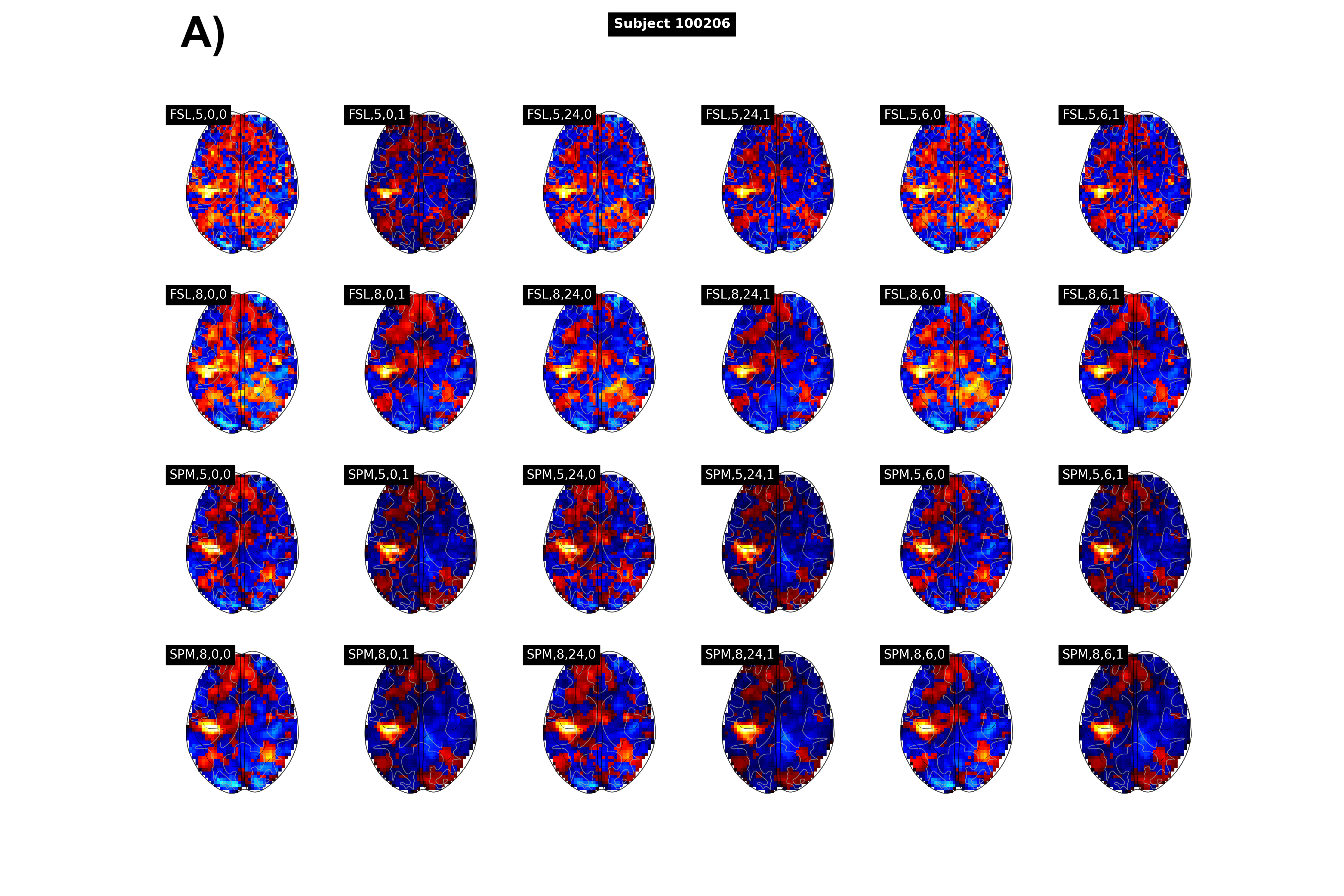
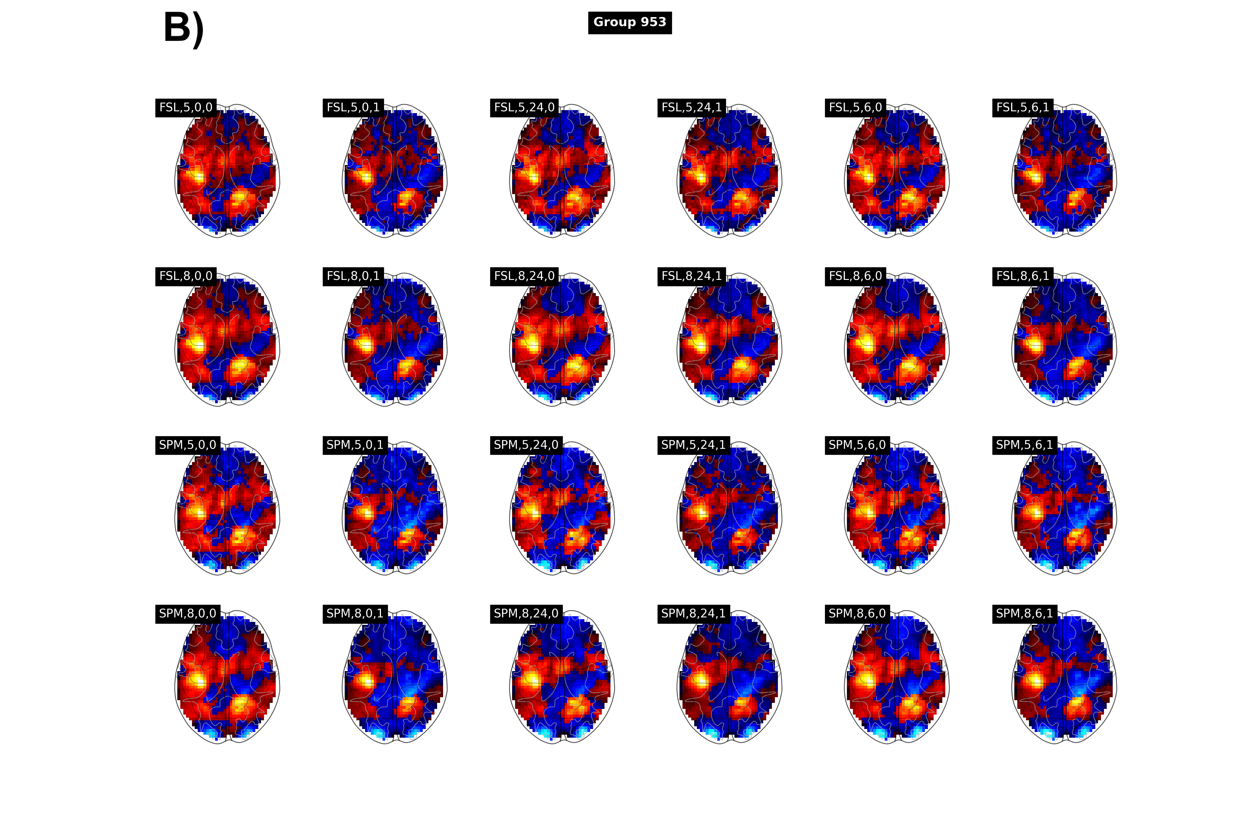
Figure 1: Example of subject (A) and group-level (B) statistic maps obtained for subject 100206 and group 953 for each pipeline for contrast right-hand. Pipelines are denoted by ‘software-FWHM-motion regressors-hrf derivatives’.

Data Records

The data will be accessible on Public nEUro [29], the preprint will be updated to include the link as soon as possible. Images were named as follows: ‘<prefix>-<id>_<contrast>_<pipeline>_<suffix>.nii.gz’ where:

• <prefix> is replaced sub and group for subject-level and group-level analyses respectively

• <id> is the identifier of the participant or the group

• <contrast> is the name of the contrast (‘right-hand’, ‘right-foot’, ‘left-hand’, ‘left-foot’, ‘tongue’)

• <pipeline> describes the pipeline (cf. Section Analyses pipelines)

• <suffix> is con for contrast maps or tstat for T-statistic maps.

For instance, sub-100206_right-hand_fsl-8-0-0_con.nii.gz is the contrast map of the subject 100206 for the contrast "right hand" and the pipeline obtained with FSL, a smoothing with a kernel FWHM of 8mm, no motion regressors and no HRF derivatives.

Technical Validation

To assess the quality of the statistic maps, we performed a quantitative analysis to estimate how well the group-level statistic maps are representative of the task performed.

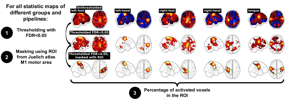
Figure 2: Workflow of technical validation of statistic maps. We thresholded each statistic map of each group, each pipeline and each contrast using a FDR of p<0.05 and masked the thresholded map using the ROI of Juelich atlas of the Primary Motor Cortex.

As described in Fig. 2, we looked at the significant activations inside the Primary Motor Cortex (M1) of the brain for each statistic map of each group, each contrast and each pipeline. Our group-level statistic maps were thresholded using a False Discovery Rate (FDR) of p<0.05 and masked using the probabilistic Juelich Atlas available in Nilearn. We selected the region of interest (ROI) corresponding to the Primary Motor Cortex, Brodmann Area 4. Depending on the contrast, both left and right hemisfer’s ROI (‘tongue’), only the left hemisfer (‘right hand’ or ‘right foot’) or only the right hemisfer (‘left hand’ or ‘left foot’) ROI were selected, to focus on controlateral activations in the motor cortex.

For each map, we computed the Percentage of activation (PA), which is the percentage of voxels of the ROI that are activated, i.e.:

$$PA=\frac{N_{activated\ voxels}}{N_{total\ voxels}}\times 100$$ (1)

where $N_{activated\ voxels}$ is the number of activated voxels in the ROI and $N_{total\ voxels}$ is the total number of voxels in the ROI.

Figure 3 represents the distribution of mean PA per contrast among all pipelines. Results were different depending on the contrast: for all contrasts, mean percentages of activation were between 20 and 40% but those of contrasts left foot and right foot were below those of right hand, left hand and tongue. When looking at the activations of different contrasts in the ROI for one of our group-level statistic maps (see Figure 4), we could see that the activations of the foot contrast seemed widespread with a small area of high activation. For a hand contrast, the high activation area was larger and covered nearly the entire ROI. This observation was consistent with the literature [30, 31] in which the identified area of activation of the foot was smaller than the hand one. In the masked thresholded statistic maps of the foot contrasts, we thus have less activated voxels. The goal of this quality check was to have a low-level estimation of the accuracy of the statistic maps to represent the task performed, thus we chose to define a single ROI covering the entire motor area. The definition of a specific ROI of the foot activation area could help having better metrics.

All pipelines shared similar metrics, with high PA for hand, cue and tongue contrasts and lower PA for foot contrasts. An example of the distribution of PA for all group maps of each contrast is shown in Figure 5 for the pipeline spm-5-0-0. The PA computed for all groups, pipelines and contrasts are available in Supplementary Files.

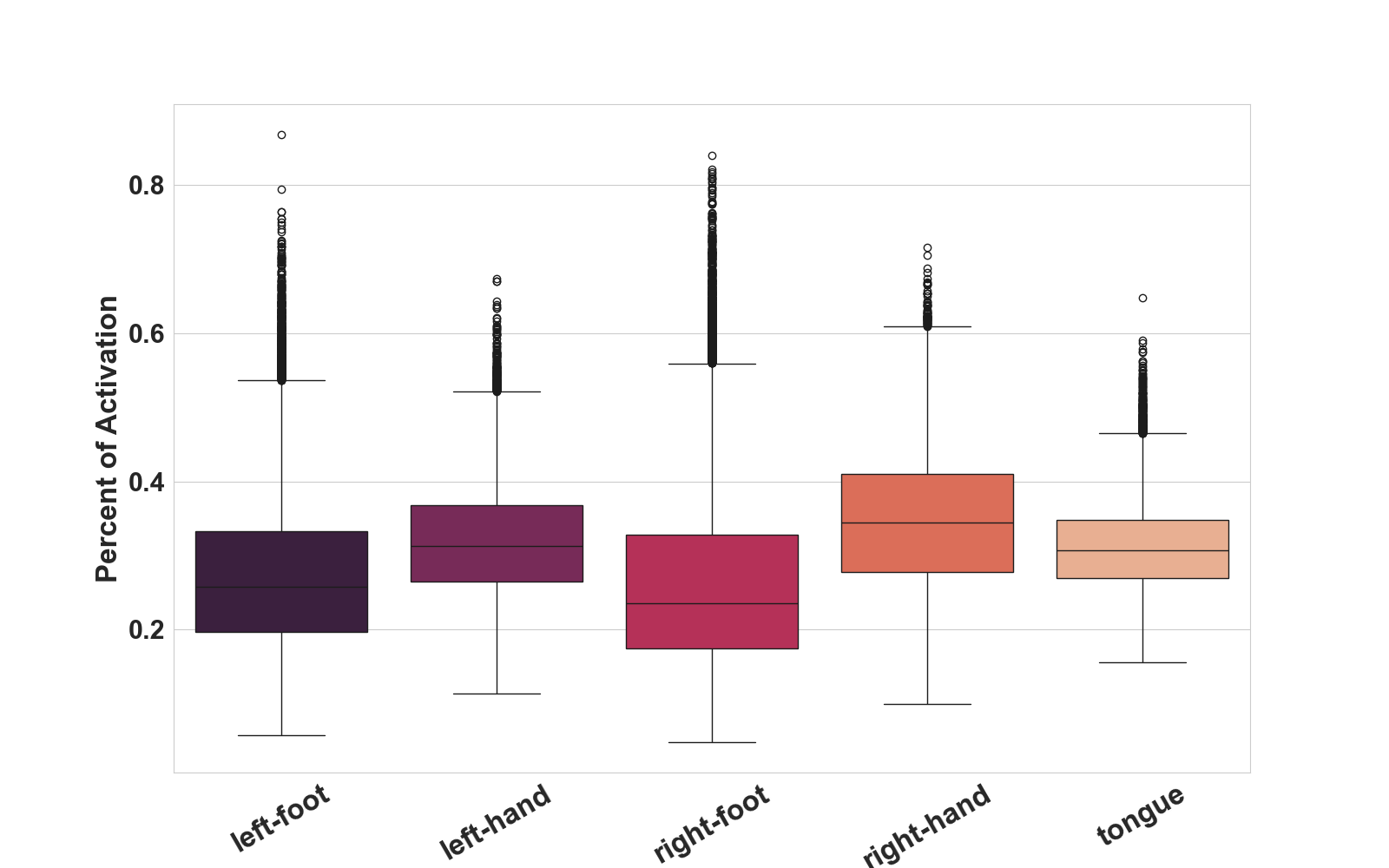
Figure 3: Distribution of mean Percentage of Activation for all groups and pipelines in the different contrast maps.

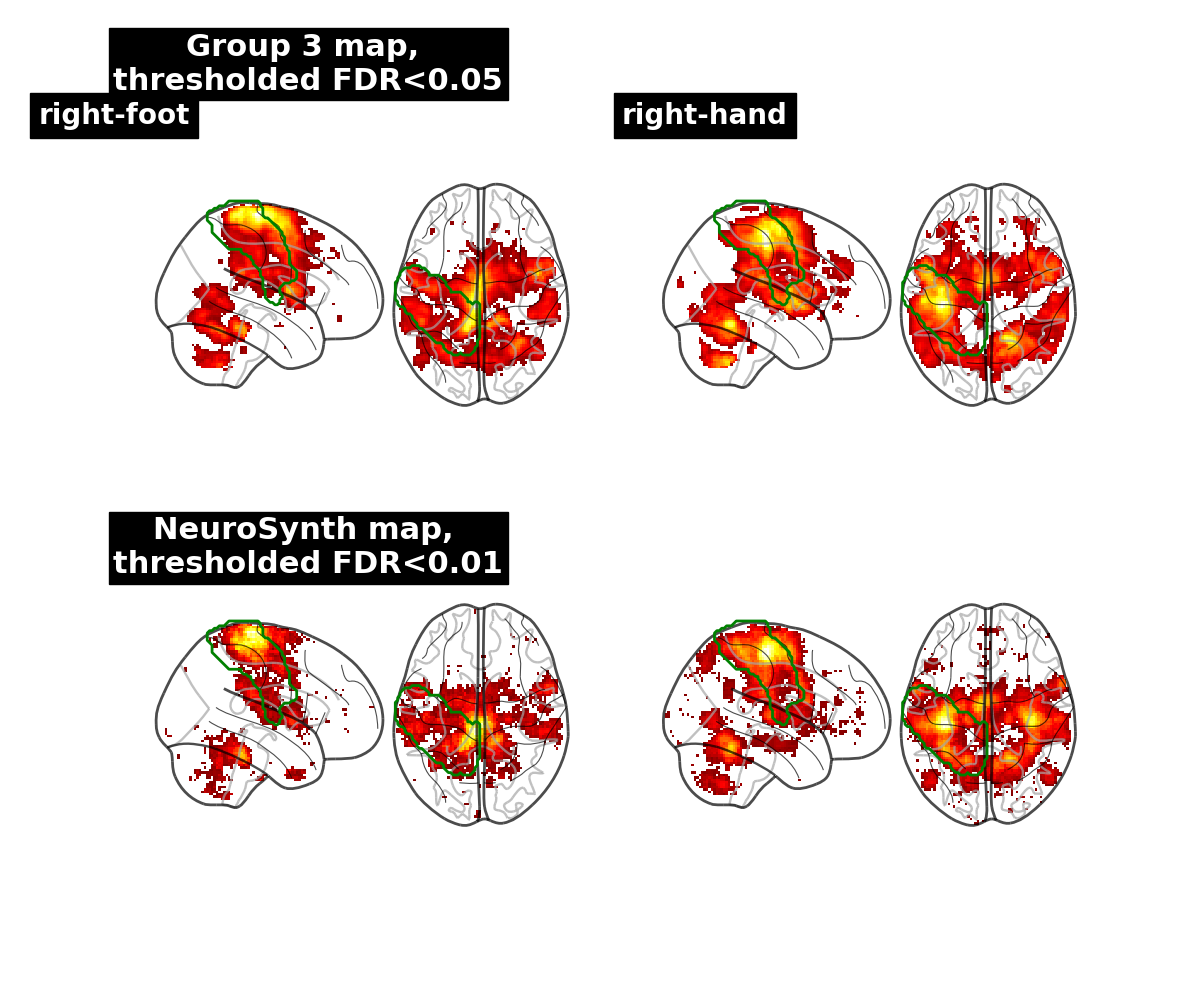
Figure 4: Thresholded statistic maps for contrasts right foot (right) and right hand (left) for group-level analysis of group 3 with pipeline spm-5-0-0 (upper). Percentage of Activation were respectively 0.34 and 0.41 for the contrasts right foot and right hand. NeuroSynth activation maps corresponding to "hand" and "foot" paradigm (lower). Green borders correspond to the motor area ROI.

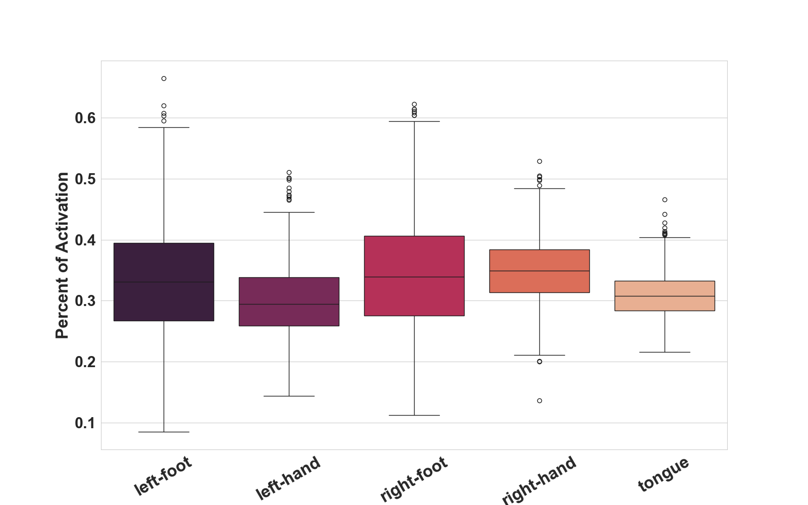
Figure 5: Distribution of Percentage of Activation for all group-level statistic maps for pipeline spm-5-0-0 in the different contrast maps.

Usage Notes

The HCP multi-pipeline dataset promotes reproducibility in neuroimaging, by providing researchers with a reusable dataset of fMRI contrast maps. The data will be accessible on Public nEUro [29], the preprint will be updated to include the link as soon as possible.

This dataset brings together a wide range of analysis conditions, covering many aspects of inter-subject, inter-groups, inter-contrasts and inter-pipelines variability. A total of 1,080 participants were used to form 1,000 different groups of 50 participants, 5 contrasts were analyzed with 24 different pipelines. Using the code provided to create the pipelines, other researchers could be able to enhance this dataset with other combinations of parameters, giving rise to other pipelines, or apply these pipelines to other participants, groups or contrasts.

While many aspects of variability have been studied in the field of neuroimaging, changes in analytical choices are still difficult to study. Due to the computational cost in time and storage capacity of analysing fMRI data, datasets dedicated to the exploration of analytical variability (i.e. in which multiple pipelines are applied to the same data) are rare. Recently, the results of the NARPS study [7] were made publicly available on NeuroVault, but even if 70 different analytic conditions were described, it only gives access to one group level statistic maps for 9 different contrasts.

Analytical variability is not limited to neuroimaging and has been studied in many other disciplines [32], such as psychology [33] or software engineering [34]. Different fields have brought solutions to explore and handle analytical variability. These techniques have begun to be used in neuroimaging, with, for instance, the implementation of continuous integration, a software engineering technique, to facilitate the reproducibility of neuroimaging computational experiments [35] or multiverse analyses that help to find the most efficient pipelines depending on the data and the goal of the study [36]. By sharing directly the results obtained from different analysis strategies, we hope to facilitate the use of these data by researchers from other fields, that could apply their own methods to explore the neuroimaging analytical space.

Code availability

All codes (analysis pipelines and technical validation) were executed in Python v3.8. The executions require the installation of SPM and FSL software packages. To facilitate reproducibility, we provide a NeuroDocker image that can be pulled from Dockerhub and that contains all necessary software packages. The Docker image is available at: https://hub.docker.com/r/elodiegermani/open_pipeline. Python scripts to create and run the pipelines as well as to perform technical validation were made available publicly at: https://archive.softwareheritage.org/swh:1:snp:17870c3d782aa25a7ffdd6165fe27ce6eac6c90b;origin=https://gitlab.inria.fr/egermani/hcp_pipelines.

Competing interests

The authors declare no competing interests.

References

- [1] Yin, W., Li, L. & Wu, F.-X. Deep learning for brain disorder diagnosis based on fMRI images. \JournalTitleNeurocomputing 469, 332–345, https://www.doi.org/10.1016/j.neucom.2020.05.113 (2022).
- [2] Firat, O., Oztekin, L. & Vural, F. T. Y. Deep learning for brain decoding. In 2014 IEEE International Conference on Image Processing (ICIP), 2784–2788, https://www.doi.org/10.1109/ICIP.2014.7025563 (IEEE, 2014).
- [3] Carp, J. On the plurality of (methodological) worlds: estimating the analytic flexibility of fMRI experiments. \JournalTitleFrontiers in Neuroscience https://www.doi.org/10.3389/fnins.2012.00149 (2012).
- [4] Penny, W., Friston, K., Ashburner, J., Kiebel, S. & Nichols, T. E. Statistical Parametric Mapping: The Analysis of Functional Brain Images (2011), elsevier edn.
- [5] Jenkinson, M., Beckmann, C. F., Behrens, T. E. J., Woolrich, M. W. & Smith, S. M. FSL. \JournalTitleNeuroImage 62, 782–790, https://www.doi.org/10.1016/j.neuroimage.2011.09.015 (2012).
- [6] Cox, R. W. AFNI: Software for Analysis and Visualization of Functional Magnetic Resonance Neuroimages. \JournalTitleComputers and Biomedical Research 29, 162–173, 10.1006/cbmr.1996.0014 (1996).
- [7] Botvinik-Nezer, R. et al. Variability in the analysis of a single neuroimaging dataset by many teams. \JournalTitleNature 582, 84–88, https://www.doi.org/10.1038/s41586-020-2314-9 (2020).
- [8] Carp, J. The secret lives of experiments: Methods reporting in the fMRI literature. \JournalTitleNeuroImage 63, 289–300, https://www.doi.org/10.1016/j.neuroimage.2012.07.004 (2012).
- [9] Klau, S. et al. Comparing the vibration of effects due to model, data pre-processing and sampling uncertainty on a large data set in personality psychology. \JournalTitleMeta-Psychology 7 (2023).
- [10] Li, X. et al. Moving beyond processing and analysis-related variation in neuroscience. 2021–12 (2021).
- [11] Xu, T. et al. A Guide for Quantifying and Optimizing Measurement Reliability for the Study of Individual Differences, 10.1101/2022.01.27.478100 (2022).
- [12] Van Essen, D. et al. The human connectome project: A data acquisition perspective. \JournalTitleNeuroImage 62, 2222–2231, https://doi.org/10.1016/j.neuroimage.2012.02.018 (2012).
- [13] Sudlow, C. et al. UK biobank: An open access resource for identifying the causes of a wide range of complex diseases of middle and old age. \JournalTitlePLOS Medicine 12, https://www.doi.org/10.1371/journal.pmed.1001779 (2015).
- [14] Glasser, M. F. et al. The minimal preprocessing pipelines for the human connectome project. \JournalTitleNeuroImage 80, 105–124, https://doi.org/10.1016/j.neuroimage.2013.04.127 (2013).
- [15] Collection nº457. NeuroVault Collection nº457. https://identifiers.org/neurovault.collection:457. Accessed: 2023-05-20.
- [16] Van Essen, D. C. et al. The wu-minn human connectome project: An overview. \JournalTitleNeuroImage 80, 62–79, https://doi.org/10.1016/j.neuroimage.2013.05.041 (2013).
- [17] Esteban, O. et al. fMRIPrep: a robust preprocessing pipeline for functional MRI. \JournalTitleNature Methods 16, 111–116, 10.1038/s41592-018-0235-4 (2019).
- [18] Human connectome project: Data usage agreement. https://www.humanconnectome.org/study/hcp-young-adult/document/wu-minn-hcp-consortium-open-access-data-use-terms.
- [19] Moeller, S. et al. Multiband multislice ge-epi at 7 tesla, with 16-fold acceleration using partial parallel imaging with application to high spatial and temporal whole-brain fmri. \JournalTitleMagnetic Resonance in Medicine 63, 1144–1153, https://doi.org/10.1002/mrm.22361 (2010).
- [20] Feinberg, D. A. et al. Multiplexed echo planar imaging for sub-second whole brain fmri and fast diffusion imaging. \JournalTitlePLOS ONE 5, 1–11, https://doi.org/10.1371/journal.pone.0015710 (2010).
- [21] Setsompop, K. et al. Blipped-controlled aliasing in parallel imaging for simultaneous multislice echo planar imaging with reduced g-factor penalty. \JournalTitleMagnetic Resonance in Medicine 67, 1210–1224, https://doi.org/10.1002/mrm.23097 (2012).
- [22] Xu, J. et al. Highly accelerated whole brain imaging using aligned-blipped-controlled-aliasing multiband epi. In Proceedings of the 20th Annual Meeting of ISMRM, vol. 2306, 1907–1913 (2012).
- [23] Gorgolewski, K. Nipype: a flexible, lightweight and extensible neuroimaging data processing framework in Python. \JournalTitleFrontiers in Neuroinformatics 15, https://www.doi.org/10.5281/zenodo.581704 (2017).
- [24] Neurodocker.
- [25] Halchenko, Y. & Hanke, M. Open is Not Enough. Let’s Take the Next Step: An Integrated, Community-Driven Computing Platform for Neuroscience. \JournalTitleFrontiers in Neuroinformatics 6, https://www.doi.org/10.3389/fninf.2012.00022 (2012).
- [26] Abraham, A. et al. Machine learning for neuroimaging with scikit-learn. \JournalTitleFrontiers in Neuroinformatics 10.3389/fninf.2014.00014 (2014).
- [27] Brett, M. et al. nipy/nibabel: 3.2.1, 10.5281/zenodo.4295521 (2020).
- [28] Woolrich, M. W., Ripley, B. D., Brady, M. & Smith, S. M. Temporal autocorrelation in univariate linear modeling of fmri data. \JournalTitleNeuroImage 14, 1370–1386, https://doi.org/10.1006/nimg.2001.0931 (2001).
- [29] Public nEUro.
- [30] Schott, G. Penfield’s homunculus: a note on cerebral cartography. \JournalTitleJ Neurol Neurosurg Psychiatry 56, 329–333, 10.1136/jnnp.56.4.329. (1993).
- [31] Yarkoni, T., Poldrack, R. A., Nichols, T. E., Van Essen, D. C. & Wager, T. D. Large-scale automated synthesis of human functional neuroimaging data. \JournalTitleNature Methods 8, 665–670, 10.1038/nmeth.1635 (2011).
- [32] Hoffmann, S. et al. The multiplicity of analysis strategies jeopardizes replicability: lessons learned across disciplines. \JournalTitleRoyal Society open science 8, 201925 (2021).
- [33] Simmons, J. P., Nelson, L. D. & Simonsohn, U. False-positive psychology: Undisclosed flexibility in data collection and analysis allows presenting anything as significant. \JournalTitlePsychological Science 22, 1359–1366, 10.1177/0956797611417632 (2011).
- [34] Alférez, M., Acher, M., Galindo, J. A., Baudry, B. & Benavides, D. Modeling variability in the video domain: language and experience report. \JournalTitleSoftware Quality Journal 27, 307–347, 10.1007/s11219-017-9400-8 (2019).
- [35] Sanz-Robinson, J., Jahanpour, A., Phillips, N., Glatard, T. & Poline, J.-B. NeuroCI: Continuous integration of neuroimaging results across software pipelines and datasets. 105–116, 10.1109/eScience55777.2022.00025 (2022).
- [36] Dafflon, J. et al. A guided multiverse study of neuroimaging analyses. \JournalTitleNature Communications 13, 3758 (2022).
Acknowledgements
This work was partially funded by Region Bretagne (ARED MAPIS) and Agence Nationale pour la Recherche for the programm of doctoral contracts in artificial intelligence (project ANR-20-THIA-0018). Data used in the HCP dataset were provided [in part] by the Human Connectome Project, WU-Minn Consortium (Principal Investigators: David Van Essen and Kamil Ugurbil; 1U54MH091657) funded by the 16 NIH Institutes and Centers that support the NIH Blueprint for Neuroscience Research; and by the McDonnell Center for Systems Neuroscience at Washington University.