On Smart Morphing Wing Aircraft Robust Adaptive Beamforming

Abstract

The smart morphing wing aircraft (SMWA) is a highly adaptable platform that can be widely used for intelligent warfare due to its real-time variable structure. The flexible conformal array (FCA) is a vital detection component of SMWA, when the deformation parameters of FCA are mismatched or array elements are mutually coupled, detection performance will be degraded. To overcome this problem and ensure robust beamforming for FCA, deviations in array control parameters (ACPs) and array perturbations, the effect of mutual coupling in addition to looking-direction errors should be considered. In this paper, we propose a robust adaptive beamforming (RAB) algorithm by reconstructing a multi-domain interference plus noise covariance matrix (INCM) and estimating steering vector (SV) for FCA. We first reconstruct the INCM using multi-domain processing, including ACP and angular domains. Then, SV estimation is executed through an optimization procedure. Experimental results have shown that the proposed beamformer outperforms existing beamformers in various mismatch conditions and harsh environments, such as high interference-to-noise ratios, and mutual coupling of antennas.

1 Introduction

Smart morphing wing aircraft (SMWA) has attracted considerable interest from scholars in the aerospace vehicle community [1, 2], due to the adaptive variable structural geometry based on the scenario and improved aerodynamic efficiency. Therefore, flexible conformal arrays (FCA), as an important part of SMWA, have received increasing attention from the research community in recent years [3, 4, 5, 6]. Due to its flexibility and conformal advantages, it allows a wide range of novel applications [7, 8, 9, 10]. For example, the physical surface of a conformal array is used to increase the effective antenna aperture, while reducing the array volume and weight. Additionally, the flexibility makes it easier for the FCA to generate the desired antenna beams for a variety of situations [8]. Emerging applications require capabilities beyond conventional static conformal arrays, such as using FCA in wearables and lightweight devices [3], deployable apertures that dynamically change shape [4]. Although FCAs can constantly change shape during deployment or operation, their element positions and mutual coupling may not be known in the practical working environment, which would result in significant performance degradation. Therefore, some robust adaptive beamforming (RAB) methods should be proposed to compensate for this degradation with respect to FCA.

As is well known, adaptive beamforming technology is very sensitive to various mismatches, such as array calibration errors, incoherent local scattering, wavefront distortion and direction-of-arrival (DOA) errors [11], resulting in significant performance degradation in the output signal-to-interference-plus-noise ratio (SINR). In addition, the adaptive beamforming method for FCA must also be robust to the inaccuracy of array control parameters (ACPs) during deformable operations of FCA, which will trigger the steering vector (SV) mismatch. Clearly, this type of error is unique to FCA, which has not been fully investigated in recent literature. Although ACP errors can be reduced to SV errors, the law of the error has not been fully discussed and the effectiveness of conventional RAB methods applied to this situation has not been investigated. Over the past decades, substantial RAB approaches have been studied [12, 13, 14, 15, 16, 17, 18, 19, 20, 21, 22, 23, 24] to mitigate the effects of model mismatches and improve beamformers’ robustness. However, the performance of these methods suffers significant performance degradation when they are applied directly to FCAs. For FCAs, the ACP errors induce severe SV mismatch, and additional looking direction error, as well as the ill interference-plus-noise covariance matrix (INCM) due to the echo signal received by time-varying geometry, which motivates us to address this thorny issue.

In general, the proposed RAB techniques can be broadly classified into four categories—diagonal loading (DL)-based ([13, 14]), eigenspace-based ([15, 16]), uncertainty set constraints-based ([17, 18]), INCM reconstruction and SV estimation-based approaches ([12, 19, 20, 24, 25]), and some other techniques ([21, 22, 23]). Inspired by [19, 23] and our previous work [6], we extend the INCM-based framework to address the FCA RAB problem. Specifically, we propose a RAB approach based on multiple domain INCM reconstruction and SV estimation in this paper to reduce the impact of ACP errors along with other types of errors (i.e., looking direction error and array perturbation). INCM is reconstructed not only on the angle domain, but also on the ACP domain, which is the extension of the method in [19]. Then, an alternative optimization scheme is proposed to estimate the true SV in the presence of ACP errors and array perturbation with mutual coupling. In short, we first reconstruct INCM with discrete summation of rank-one matrix in angle and ACP domains, and then estimate SV by solving two alternative optimization problems. The true SV is composed of two terms, one term is the orthogonal component that can be estimated by a QCQP problem, and the other term is the perturbation component that can be estimated by solving a barrier function using the internal point method.

The rest of the paper is organized as follows: Section II introduces the FCA geometry and signal model with mutual coupling effects, and summarizes the FCA optimization object in case of mixed mismatches in practice. Next, the RAB algorithm is proposed in Section III. Numerical simulations of three scenarios are provided in Section IV and conclusions are drawn in Section V.

notations: $\odot$ represents the Hadamard Product, $\mathrm{diag}\left\{\cdot\right\}$ denotes the diagonalize matrix of brace. $\left(\bullet\right)^{T}$ and $\left(\bullet\right)^{H}$ denote the transpose and Hermitian transpose, respectively. $E\left\{\bullet\right\}$ is the statistical expectation. $|\bullet|$ is the absolute value, and $\left\|\bullet\right\|_{2}$ is the norm-2 of the vector or matrix.

2 Signal Model of FCA

SMWA will change wing shape according to different combat scenarios, flight phases, and enemy aircraft types and specifications. For example, when a radar needs to detect or evade a target, a larger or smaller array aperture is required accordingly, so the SMWA need control the wing for timely expansion or contraction, as shown in Fig.1. After being elongated and shortened, the spacing of the array element will become uneven, and specifically, the maximum pointing direction of the beam pattern is deflected and the sidelobe level rises sharply, which is shown at the bottom of Fig.1. The corresponding beampattern will inevitably deteriorate in transmission and reception patterns. However, the existing RAB method has serious performance losses when dealing with ACP errors of FCA. Therefore, we need to propose a RAB method for the presence of ACP errors so that FCA can work properly.

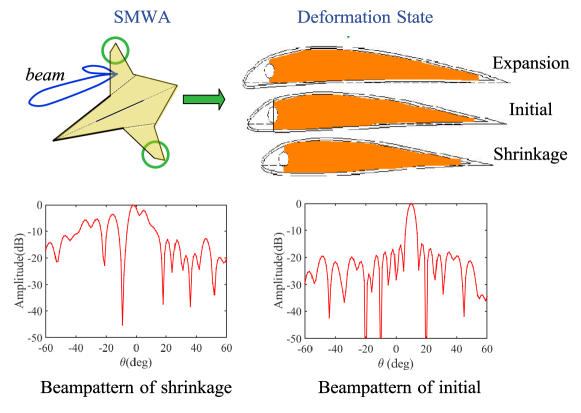
Figure 1: The deformation scenarios of SMWA and corresponding beampatterns.

In view of this, we present a FCA wing geometry as shown in Fig. 2. The elements are uniformly distributed over two splice rings with half-wavelength inter-element spacing (in this case it means geodesic distance), and the elements have the same isotropic pattern with known positions. The ACPs are the two radiuses of the splice rings (i.e., $R_{1}$ and $R_{2}$), illustrating that the radiuses can be increased or decreased in the operation of the deformable surface. This model can be used to simulate airfoil adjustments such as camber deformation and thickness corresponding to SMWA [1].

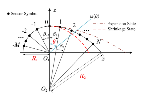
Figure 2: The configuration of flexible conformal array with two controlling parameters

Further, suppose that the array of $M+N$ sensors receives signals from multiple narrowband sources. Let $S=M+N$ represents the total number of all elements. The array observation vector $\mathbf{x}\left(k\right)\in\mathbb{C}^{S\times 1}$ at time $k$ can be modeled as

$$\mathbf{x}\left(k\right)=\mathbf{x}_{s}\left(k\right)+\mathbf{x}_{i}\left(k\right)+\mathbf{x}_{n}\left(k\right),$$ (1)

where $\mathbf{x}_{s}\left(k\right)$, $\mathbf{x}_{i}\left(k\right)$, and $\mathbf{x}_{n}\left(k\right)$ are the statistically independent components of the desired signal, interference, and noise, respectively. Another, consider the wavefield generated by one desired and $L-1$ interference sources located at $\left\{\theta_{1},\theta_{2},\cdots,\theta_{L}\right\}$, so that the desired signal $\mathbf{x}_{s}\left(k\right)$ and interference $\mathbf{x}_{i}\left(k\right)$ can be written as

$$\mathbf{x}_{s}\left(k\right)= \boldsymbol{C}\mathbf{a}\left(\theta_{1}\right)s_{1}\left(k\right)$$ (2)

$$\mathbf{x}_{i}\left(k\right)= \sum\nolimits_{j=2}^{\mathrm{L}}{\boldsymbol{C}\mathbf{a}\left(\theta_{j}\right)s_{j}\left(k\right)},$$ (3)

where $s_{j}\left(k\right)$ is the sample transmitted by $j^{th}$ source and $\mathbf{a}\left(\theta_{j}\right)\in\mathbb{C}^{S\times 1}$ is the complex SV associated with the source signal located at ${\theta_{j}}$. $\boldsymbol{C}\in\mathbb{C}^{S\times S}$ is mutual coupling matrix (MCM), and $\mathbf{x}_{n}\left(k\right)\in\mathbb{C}^{S\times 1}$ is the complex vector of ambient channel noise samples that subject to Gaussian distribution in general. Then

$$\mathbf{x}\left(k\right)=\sum\nolimits_{j=1}^{\mathrm{L}}{\boldsymbol{C}\mathbf{a}\left(\theta_{j}\right)s_{j}\left(k\right)+\mathbf{x}_{n}\left(k\right)}.$$ (4)

Equation (4) can be simplified by defining the effective array SV as [26]

$$\mathbf{\tilde{a}}\left(\theta_{j}\right)=\boldsymbol{C}\mathbf{a}\left(\theta_{j}\right).$$ (5)

Note that the matrix $\boldsymbol{C}$ can be estimated by array calibration methods in [27] or directly measuring the effective array pattern [28], as it assumed to be independent of the DOA of signal [29]. Due to the flexibility of the FCA, the MCM varies with each deformation operation and should be considered in the algorithm. However, it is not convenient to measure MCM (e.g. full-wave simulation software HFSS) timely. Thus, a trade-off method is adopted to maintain the adaptivity of our approach. The mutual coupling between elements weakens with increasing spacing, and when the spacing is sufficiently large, the effect can be ignored [29]. Therefore, we only need to calculate it in small spacing state (e.g., when element spacing less than $2\lambda$, where $\lambda$ is the wavelength of radiation frequency), and assume $\boldsymbol{C}=\boldsymbol{I}$ ($\boldsymbol{I}$ is the identity matrix) in other cases. Accordingly, each MCM of several selected states can be measured offline, and then approximated MCM will be called in real time for ABF processing. In this paper, the MCM is estimated using HFSS with a carefully selected set of ACPs.

The typical adaptive beamformer output is given by [11]

$$y\left(k\right)=\mathbf{w}^{H}\mathbf{x}\left(k\right)$$ (6)

where $\mathbf{w}=\left[w_{1},\cdots,w_{S}\right]^{T}\in\mathbb{C}^{S\times 1}$ is the beamformer weighted vector.

Considering the mutual coupling effect, $\mathbf{w}$ can be obtained by maximizing the output SINR, which is known as the Capon beamformer[11],

$$\mathbf{w}_{\mathrm{opt}}=\frac{\mathbf{R}_{i+n}^{-1}\mathbf{\tilde{a}}\left(\theta_{1}\right)}{\mathbf{\tilde{a}}^{H}\left(\theta_{1}\right)\mathbf{R}_{i+n}^{-1}\mathbf{\tilde{a}}\left(\theta_{1}\right)}$$ (7)

where $\mathbf{\tilde{a}}\left(\theta_{1}\right)$ is the presumed efficient array SV of $\theta_{1}$ direction, $\mathbf{R}_{i+n}\triangleq E\{(\mathbf{x}_{i}\left(k\right)+\mathbf{x}_{n}\left(k\right))(\mathbf{x}_{i}\left(k\right)+\mathbf{x}_{n}\left(k\right))^{H}\}\in\mathbb{C}^{S\times S}$ is the interference-plus-noise covariance matrix (INCM). In practice, $\mathbf{R}_{i+n}$ is usually unavailable even in signal-free applications, so it is replaced by the sample covariance matrix (SCM), i.e., $\mathbf{\hat{R}}={{1}/{K}}\sum\nolimits_{k=1}^{K}{\mathbf{x}\left(k\right)\mathbf{x}^{H}\left(k\right)}$ with $K$ snapshots, and the corresponding adaptive beamformer is the so-called sample matrix inversion (SMI) beamformer.

Compared to the regular linear or planner array, the beamforming performance of FCA is inherently affected by a considerable facets such as ACP errors and SV mismatches. This impart complexity and susceptibility into RAB by the extra flexibility. Consider the practical application scenario, there always exists the mismatch of SV caused by the error of CP during each deformable operations of the FCA. According to the specific FCA model shown in Fig.2, the SV can be denoted as,

$$\mathbf{a}\left(\theta_{i},r_{1},r_{2}\right)=\left[\begin{matrix}e^{jk\boldsymbol{p}_{1}\left(r_{1},r_{2}\right)\cdot\boldsymbol{u}\left(\theta_{i}\right)}&\cdots&e^{jk\boldsymbol{p}_{S}\left(r_{1},r_{2}\right)\cdot\boldsymbol{u}\left(\theta_{i}\right)}\\ \end{matrix}\right]^{T}$$ (8)

Here, $r_{1}$ and $r_{2}$ are two independent random variables representing the true values of $R_{1}$ and $R_{2}$, which fluctuate over small ranges. ${\boldsymbol{u}}(\theta_{i})$ denotes the unit vector of the impinging direction of the source in $\theta_{i}$, i.e., $\boldsymbol{u}\left(\theta_{i}\right)=\left[\begin{matrix}\sin\theta_{i}&\cos\theta_{i}\\ \end{matrix}\right]^{T}$. $\boldsymbol{p}_{1},\cdots,\boldsymbol{p}_{S}$ denote the nominal location of each element respectively, i.e. $\boldsymbol{p}_{s}=r_{1}\left[\begin{matrix}\sin\mathrm{(}\beta_{s})&\cos\mathrm{(}\beta_{s})\\ \end{matrix}\right]^{T}$, if $s=-1,\cdots,-M$, and $\boldsymbol{p}_{s}=r_{1}\left[\begin{matrix}0&1\\ \end{matrix}\right]^{T}+r_{2}\left[\begin{matrix}\sin\mathrm{(}\beta_{s})&\cos\mathrm{(}\beta_{s})-1\\ \end{matrix}\right]^{T}$, if $s=1,\cdots,N$, and $\beta_{s}$ represents the angle at the center of the circle $O_{1}$ or $O_{2}$, which can determine the position of each element. Usually, $\beta_{s}=s\lambda/\left(2R_{1}\right),s=-1,\cdots,-M$, and $\beta_{s}=s\lambda/\left(2R_{2}\right),s=1,\cdots,N$, where $R_{1}$ and $R_{2}$ are the initial values.

Another, we assume $\left|r_{1}-\bar{r}_{1}\right|\leqslant l_{1},\left|r_{2}-\bar{r}_{2}\right|\leqslant l_{2}$. $\bar{r}_{1}$ and $\bar{r}_{2}$ are the presumed values of ACPs, $l_{1}$ and $l_{2}$ are two real numbers representing the maximum errors of ACPs. In practice, the true values of ACPs cannot be measured precisely. In addition, the information at the arrival angle of the signal of interest (SOI) may be imprecise, and the knowledge of the array location maybe inaccurate or unreliable due to array calibration errors, vibrations and sensory errors. In particular, the SMI mismatch caused by a small snapshot should also be considered. Thus, from a holistic perspective, a more comprehensive optimal RAB problem for FCA is described as

$$\left\{\begin{array}[]{l}\underset{\mathbf{w}}{\min}\,\,\mathbf{w}^{H}\mathbf{R}_{i+n}\mathbf{w}\\ s.t.\,\,\,\left|\mathbf{w}^{H}\mathbf{a}\left(\theta,r_{1},r_{2}\right)\right|\geqslant 1,\left|\theta-\theta_{1}\right|\leqslant\delta_{\theta}\\ \qquad\left|r_{1}-\bar{r}_{1}\right|\leqslant l_{1},\left|r_{2}-\bar{r}_{2}\right|\leqslant l_{2}\\ \qquad\mathbf{a}\left(\theta,r_{1},r_{2}\right)\in\mathcal{A}\left(\mathbf{a}\left(\theta,r_{1},r_{2}\right)\right)\\ \end{array}\right.$$ (9)

Here, $\delta_{\theta}$ is a small number that represents the error in the DOA. Due to the perturbation of the array elements induced by the above reasons, the actual signal SV usually belongs to the uncertainty set $\mathcal{A}\left(\mathbf{a}\left(\theta,r_{1},r_{2}\right)\right)\subset\mathbb{C}^{S\times 1}$, which is defined as

$$\mathcal{A}\left(\mathbf{a}\left(\theta,r_{1},r_{2}\right)\right)=\left\{\boldsymbol{c}\left|\boldsymbol{c}=\mathbf{a}\left(\theta,r_{1},r_{2}\right)+\boldsymbol{e},\left\|\boldsymbol{e}\right\|_{2}\leqslant\varepsilon\right.\right\}$$ (10)

where $\varepsilon>0$ is a known constant which is bounded by the 2-norm of SV distortion. If we know some prior information about SV mismatch, (10) can be reformulated as an ellipsoid uncertainty set, for more details see [30].

3 THE PROPOSED METHOD

For regular structure arrays, there are many approaches to dealing with the RAB problems which are discussed in [31],[23], and[32]. However, the performance of the aforementioned algorithms will degrade when they are applied to FCA due to its unique structure and radiation properties. Therefore, a RAB algorithm based on extended multi-domain INCM reconstruction and SV estimation is proposed for FCA to compensate the errors of ACPs in this paper.

3.1 INCM reconstruction

In general, the INCM is reconstructed by calculating the integral of the spatial spectrum distribution over all possible directions that refer to the spatial domain except the hypothetical direction (SOI spatial direction) [19]. For FCA, this domain is extended to an extra parameter domain that is different from the algorithms proposed in [19] and [33]. In detail, considering the mutual coupling effect, the INCM represented by $\hat{\boldsymbol{R}}_{i+n}$ is reconstructed as

$$\hat{\boldsymbol{R}}_{i+n}=\hat{\sigma}_{n}^{2}\mathbf{I}+\sum\nolimits_{q=1}^{T-1}{\iiint\limits_{V_{\mathbf{a}}\left(q\right)}{\frac{\boldsymbol{C}\mathbf{aa}^{H}\boldsymbol{C}^{H}}{\mathbf{a}^{H}\boldsymbol{C}^{H}\hat{\boldsymbol{R}}^{-1}\boldsymbol{C}\mathbf{a}}}d\mathbf{a}}$$ (11)

where $\hat{\sigma}_{n}^{2}$ is the estimated noise power which usually equals to the minimal eigenvalue of $\hat{\boldsymbol{R}}$. $V_{\mathbf{a}}\left(q\right)$ is the uncertainty domain in $\mathbb{C}^{S\times 1}$ corresponding to the $q$-th interference, denoted as

$$V_{\mathbf{a}}\left(q\right) =\left\{\boldsymbol{a}\mid\left\|\boldsymbol{a}-\mathbf{a}\left(\theta_{q},r_{1},r_{2}\right)\right\|_{2}\leqslant\varpi,\right.$$ (12)

$$\qquad\left.\left|r_{1}-\bar{r}_{1}\right|\leqslant l_{1},\left|r_{2}-\bar{r}_{2}\right|\leqslant l_{2},\theta_{q}\in\Theta_{q}\right\}$$

where $\theta_{q}$ is the presumed direction of $q$-th interference, and $\Theta_{q}$ is the corresponding range induced by the inaccurate estimation of the direction. $\varpi$ constrains the possible SV with a sphere in high dimensional complex space $\mathbb{C}^{S\times 1}$. Fig.3 shows an intuitive explanation of the $V_{\mathbf{a}}\left(q\right)$ and the corresponding point in $\mathbb{C}^{S\times 1}$ space.

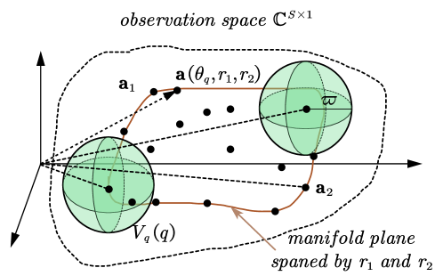
Figure 3: Graphical representation of the array manifold cube in $\mathbb{C}^{S\times 1}$, $\mathbf{a}_{1}$ and $\mathbf{a}_{2}$ are the representations of possible SV which are denoted by carbon spots.

Note that, although it is easy to find the parallel and orthogonal component of a specified SV (i.e., divide $V_{\mathbf{a}}\left(q\right)$ into many vector sets) in complex space, it is difficult to calculate the integral in that space. Thus we choose to approximate (11) by calculating the discrete sum as

$$\hat{\boldsymbol{R}}_{i+n}=\hat{\sigma}_{n}^{2}\mathbf{I}+\frac{4l_{1}l_{2}}{S_{r_{1}}S_{r_{2}}}\sum_{q=1}^{T-1}{\frac{L_{\varTheta}}{S_{\Theta_{q}}}\sum_{r_{1}}{\sum_{r_{2}}{\sum_{\theta}{\frac{\boldsymbol{C}\mathbf{aa}^{H}\boldsymbol{C}^{H}}{\mathbf{a}^{H}\boldsymbol{C}^{H}\hat{\boldsymbol{R}}^{-1}\boldsymbol{C}\mathbf{a}}}}}}$$ (13)

where ${S_{r_{1}},S_{r_{2}},S_{\Theta_{q}}}$ represents the corresponding sampling number in parameter range, respectively. $L_{\varTheta}$ represents the length of interval $\Theta_{q}$.

3.2 SV estimation using Alternative optimization

Assume the real SV can be denoted as

$$\mathbf{a}=\bar{\mathbf{a}}\left(\theta_{1},r_{1},r_{2}\right)+\mathbf{e}_{\bot}$$ (14)

where $\mathbf{\bar{a}}\left(\theta_{1},r_{1},r_{2}\right)$ is the presumed SV of SOI with parameter $\left(\theta_{1},r_{1},r_{2}\right)$, which is a function of ACPs due to the special feature of FCA. $\mathbf{e}_{\bot}$ is one component of the mismatch vector $\mathbf{e}$, which is orthogonal to $\mathbf{\bar{a}}$. Then, we estimate the SV of SOI by solving the following optimization problem,

$$\left\{\begin{aligned} \underset{r_{1},r_{2},\mathbf{e}_{\bot}}{\min}&\,\,\left(\bar{\mathbf{a}}\left(\theta_{1},r_{1},r_{2}\right)+\mathbf{e}_{\bot}\right)^{H}\grave{\boldsymbol{R}}\left(\bar{\mathbf{a}}\left(\theta_{1},r_{1},r_{2}\right)+\mathbf{e}_{\bot}\right)\\ s.t.\quad&\bar{\mathbf{a}}^{H}\mathbf{e}_{\bot}=0,\bar{\mathbf{a}}\in V_{\mathbf{a}}\left(1\right)\\ &\left(\bar{\mathbf{a}}+\mathbf{e}_{\bot}\right)^{H}\grave{\boldsymbol{R}}\left(\bar{\mathbf{a}}+\mathbf{e}_{\bot}\right)\leqslant\bar{\mathbf{a}}^{H}\grave{\boldsymbol{R}}\bar{\mathbf{a}}\\ \end{aligned}\right.$$ (15)

For simplicity, $\grave{\boldsymbol{R}}=\boldsymbol{C}^{H}\hat{\boldsymbol{R}}^{-1}\boldsymbol{C}$, and the dependence of various vectors and matrices on the variable will be dropped and only explicitly mentioned when needed (in this case $\bar{\mathbf{a}}$ denotes $\bar{\mathbf{a}}\left(\theta_{1},r_{1},r_{2}\right)$). The other component is parallel to $\mathbf{\bar{a}}$ which is omitted here because beamforming quality will not be affected by a scaled copy of it. Then, the equality constraint is introduced to maintain orthogonality between them, and the inequality constraint is aimed at preventing the actual SV from converging to any interference in the range of SOI.

Note that (15) is a multivariate nonconvex optimization problem, using the idea of alternating direction multipliers (ADMM) [34], (15) can be factorized into two alternative optimization problems (see Appendix 5.1 for detailed deduction):

$$p_{1}^{\left(m\right)}:\left\{\begin{aligned} &\underset{\mathbf{e}_{\bot}}{\min}\,\,(\bar{\mathbf{a}}^{\left(m-1\right)}+\mathbf{e}_{\bot})^{H}\grave{\boldsymbol{R}}(\bar{\mathbf{a}}^{\left(m-1\right)}+\mathbf{e}_{\bot})\\ &s.t.\quad{\mathbf{e}^{H}}_{\bot}\bar{\mathbf{a}}^{\left(m-1\right)}=0,\\ &\qquad(\bar{\mathbf{a}}^{\left(m-1\right)}+\mathbf{e}_{\bot})^{H}\grave{\boldsymbol{R}}(\bar{\mathbf{a}}^{\left(m-1\right)}+\mathbf{e}_{\bot})\\ &\qquad\qquad\qquad\quad\leqslant(\bar{\mathbf{a}}^{\left(m-1\right)})^{H}\grave{\boldsymbol{R}}\bar{\mathbf{a}}^{\left(m-1\right)}\\ \end{aligned}\right.$$ (16)

and

$$p_{2}^{\left(m\right)}:\left\{\begin{aligned} &\underset{r_{1},r_{2}}{\min}\,\,(\bar{\mathbf{a}}+\mathbf{e}_{\bot}^{\left(m\right)})^{H}\grave{\boldsymbol{R}}(\bar{\mathbf{a}}+\mathbf{e}_{\bot}^{\left(m\right)})\\ &s.t.\quad\bar{\mathbf{a}}^{H}\mathbf{e}_{\bot}^{\left(m\right)}=0,\left|r_{1}-\bar{r}_{1}\right|\leqslant l_{1},\left|r_{2}-\bar{r}_{2}\right|\leqslant l_{2}\\ &\qquad(\bar{\mathbf{a}}+\mathbf{e}_{\bot}^{\left(m\right)})^{H}\grave{\boldsymbol{R}}(\bar{\mathbf{a}}+\mathbf{e}_{\bot}^{\left(m\right)})\leqslant\bar{\mathbf{a}}^{H}\grave{\boldsymbol{R}}\bar{\mathbf{a}}\\ \end{aligned}\right.$$ (17)

where $m=1,2,3\cdots$ is the iterative index. Note that, $p_{1}^{\left(m\right)}$ is a QCQP problem if we fix $\bar{\mathbf{a}}$, which can be solved using convex optimization software, such as CVX [35]. Then we focus on $p_{2}^{\left(m\right)}$, because the optimization variables (i.e., $r_{1}$ and $r_{2}$) are in the exponent part. It is difficult to deal with this nonconvex optimization problem. So we resort to inner point method [36]. By this we can alternatively solve the two optimization problems equivalently in order to solve (15) .

For the convergence of the proposed alternative optimization method, we know that $\bar{\mathbf{a}}+\mathbf{e}_{\bot}$ is convergent because $\mathbf{e}_{\bot}$ is constrained by quadratic constraints and the norm-2 of $\bar{\mathbf{a}}$ is constant.

After $M_{r}$ iterations, the optimal result of $p_{1}^{\left(m\right)}$ and $p_{2}^{\left(m\right)}$ converge to $\mathbf{e}_{\bot}^{*}$ and $\bar{\mathbf{a}}^{*}$, respectively. Then substitute them and (13) into the Capon beamformer (7), we obtain the optimal beamformer as

$$\mathbf{w}^{md}=\frac{\hat{\boldsymbol{R}}_{i+n}^{-1}\boldsymbol{C}\left(\bar{\mathbf{a}}^{*}+\mathbf{e}_{\bot}^{*}\right)}{\left(\bar{\mathbf{a}}^{*}+\mathbf{e}_{\bot}^{*}\right)^{H}\boldsymbol{C}^{H}\hat{\boldsymbol{R}}_{i+n}^{-1}\boldsymbol{C}\left(\bar{\mathbf{a}}^{*}+\mathbf{e}_{\bot}^{*}\right)}$$ (18)

The proposed algorithm is summarized in Algorithm 1.

Algorithm 1 Proposed robust beamforming algorithm for FCA.

1:

2:$\hat{\boldsymbol{R}}$ ;$\mathbf{\bar{a}}^{\left(0\right)}$; $\varpi$; $\bar{r}_{1},\bar{r}_{2},l_{1},l_{2}$; $\boldsymbol{C}$;

3:The parameter sequence of barrier weight: $\varepsilon^{\left(k\right)}$;

4:The iterative stopping condition: $\tau_{x},\tau_{y},\tau_{\boldsymbol{e}},D$.

5:$\bar{\mathbf{a}}^{*}$ ; $\mathbf{e}_{\bot}^{*}$; $\hat{\boldsymbol{R}}_{i+n}$.

6:Determine the discrete sampling set of parameters corresponding to each sources (totally $L$ terms), i.e., $\left(\theta,r_{1},r_{2}\right)\in\mathop{\underbrace{\left\{\theta_{1},\cdots\right\}}}\limits_{S_{\theta}}\times\mathop{\underbrace{\left\{\bar{r}_{1},\cdots\right\}}}\limits_{S_{r_{1}}}\times\mathop{\underbrace{\left\{\bar{r}_{2},\cdots\right\}}}\limits_{S_{r_{2}}}$, and to reconstruct: $\boldsymbol{\hat{R}}_{i+n}$ using (13);

7:initialize $m=1$ and $\mathbf{\bar{a}}=\mathbf{\bar{a}}^{\left(0\right)}$;

8:Solving the optimization problem $p_{1}^{\left(m\right)}$ using CVX, and obtaining the optimal result of $\mathbf{e}_{\bot}^{\left(m\right)}$;

9:Set $\mathbf{e}_{\bot}=\mathbf{e}_{\bot}^{\left(m\right)}$; and solve the optimization problem $p_{2}^{\left(m\right)}$ by inner point method and Newton’s method (using (31)) to obtain $x^{(m)},y^{(m)}$ and $\bar{\mathbf{a}}^{\left(m\right)}$;

10:If $\left|x^{(m)}-x^{(m-1)}\right|\leqslant\tau_{x},\left|y^{(m)}-y^{(m-1)}\right|\leqslant\tau_{y},\left\|\mathbf{e}_{\bot}^{\left(m\right)}-\mathbf{e}_{\bot}^{\left(m-1\right)}\right\|_{2}\leqslant\tau_{\boldsymbol{e}}$; or $m>D$, go to step 12.

11:else set $m:=m+1$ and go to step 8;

12:return $\boldsymbol{\hat{R}}_{i+n}$, $\bar{\mathbf{a}}^{*}$, $\mathbf{e}_{\bot}^{*}$.

3.3 COMPLEXITY ANALYSIS

Suppose we only consider the numbers of multiplication operations (MOs). Table 1 illustrates the required number of MOs for several mathematical operations (see [39]).

Table 1: Required number of MOs for typical mathematical operations

Operation	Required number of MOs
Exponential($e^{x}$)	15
Sin($x$)	7
Cos($x$)	8
Complex multiplication	6
Matrix multiplication($\boldsymbol{A}_{m\times n}\boldsymbol{B}_{n\times d}$)	$m\cdot n\cdot d$
Matrix inversion($\boldsymbol{A}_{n\times n}$)	$\mathcal{O}\left(n^{3}\right)$
SVD decomposition	$\mathcal{O}\left(n^{3}\right)$
QCQP problem($n$ is order)[40]	$\mathcal{O}\left(n^{3}\right)$

1. INCM reconstruction: Assuming the iteration number of SV estimation is $Q_{s}$, for one iteration of it, we have:

   • $\boldsymbol{\hat{R}}_{i+n}$ needs $4LS^{2}S_{\theta}S_{r_{1}}S_{r_{2}}$ MOs.

   • To estimate $\bar{\mathbf{a}}^{\left(m\right)}$, we need $\mathcal{O}\left(S^{3}\right)$ MOs.

   • To estimate $\mathbf{e}_{\bot}^{\left(m\right)}$ by solving QCQP, we need $\mathcal{O}\left(S^{3}\right)$ MOs.

2. Hence, the total complexity for TS-SQP is

   $$\begin{cases}\mathcal{O}\left(S^{3}Q_{s}\right),\,\,if\,\,S\gg S_{ma}\\ \mathcal{O}\left(S_{ma}^{3}S\right),\,\,if\,\,S_{ma}\gg S\\ \end{cases}$$ (19)

   where we take the notation of $S_{ma}=max\{Q_{s},S_{r_{1}},S_{r_{2}},S_{r_{\theta}}\}$.

4 SIMULATION RESULT

Consider 23-element FCA ($M=9,N=13$, and $R_{1}=500\left(mm\right)$, $R_{2}=1000\left(mm\right)$) with fixed central angle $\beta_{-1}=-\lambda/(2R_{1})$ or $\beta_{1}=\lambda/(2R_{2})$, respectively, as shown in Fig.2. The desired direction is $\theta_{1}=10\degree$. There are three equipowered interferers located at $-20^{\degree}$, $-10^{\degree}$ and $20^{\degree}$, and the signal noise ratio (SNR) is 30dB. The additive noise is modeled as a Gaussian zero-mean spatial and temporal white process.

To obtain the mutual coupling matrix $\boldsymbol{C}$, the impedance matrix $\boldsymbol{Z}$ is obtained using HFSS software and then calculated by

$$\boldsymbol{C}=\left(Z_{A}+Z_{T}\right)\left(\boldsymbol{Z}+Z_{T}\boldsymbol{I}\right)^{-1}.$$ (20)

where $Z_{A}+Z_{T}=2Re\left\{diag\left(\boldsymbol{Z}\right)\right\}$, $Re\left\{\bullet\right\}$ is the real part of brace. The angular region of one desired signal is set to be $\varTheta=\left[\theta_{1}-5{\degree},\theta_{1}+5{\degree}\right]$, and the same range is used by each interference, while the complementary angular sectors of $\varTheta$ are $\bar{\varTheta}=\left[-90{\degree},\theta_{1}-5{\degree}\right]\cup\left[\theta_{1}+5{\degree},90{\degree}\right]$ in order to implement classical INCM reconstruction beamformer. All integral operations in this paper are replaced by discrete sums and all angular sectors are uniformly sampled with the same angular interval $0.5\degree$. For each scenario, 100 Monte-Carlo runs are performed.

The performance of the proposed algorithm is compared with: diagonal loading method (DL-SMI) proposed in [26], eigenspace projection methods ( Eigenspace) in [16], norm and uncertainty set constrained method (DCRCB) in [11] and the classical INCM reconstruction and SV estimation method (Reconstruct) in [19].

For the proposed beamformer, we set $(\tau_{x},\tau_{y},\tau_{\boldsymbol{e}})=(0.01,0.1,0.1)$ and carefully design $\epsilon^{k}=\left(100,\cdots,1\right)$ with 10 terms uniformly. Convex optimization toolbox CVX [35] is used to solve optimization problems.

4.1 Example1: Mismatch due to ACP Errors

In the first example, we simulate a scenario where the actual ACPs of the FCA are not exactly known and the mutual coupling effect is ignored. We set the fixed errors of ACPs, $\varDelta R_{1}=-0.21\,mm$, $\varDelta R_{2}=3.7\,mm$. Fig.4 shows the output SINR curves of the tested methods versus the input SNR for the fixed snapshot $K=2S=46$. It shows that the proposed method achieves better performance than Eigenspace and INCM reconstruct methods, etc. It is worth noting that the curve of the Eigenspace beamformer is close to the proposed one at low SNR, but it suffers degradation in high input SNR conditions. Because the proposed method greatly benefits the highly accurate estimations of both the SV of SOI and INCM, its performance is very close to the optimal curve. Whereas the Reconstruct method suffers performance degradation because it does not consider this fact. Moreover, Fig.4 has shown that a small error of ACPs ($\varDelta R_{1}=-0.21\,mm$ compared to $R_{1}=500\,mm$) induce a significant loss of output SINR, since there is a gap of 10dB approximately between the curves of the proposed and INCM reconstruction methods. Due to the existence of ACPs error, the DCRCB method can not fully cover the range of the real SV, so the performance is always poor. The performance of DL-SMI decreases with the increase of input SNR because it can not accurately estimate the loading factor and the SCM when SNR is high.

In order to show the interference rejection performance of the proposed method intuitively, we compare our method with the Eigenspace method, which performs similarly to our proposed method. It is clear from Fig.5 that the proposed beamformer provides the highest desired signal beam at $10\degree$ and has the deepest nulls at DOAs (i.e., -10°, -20°, 20°) compared with the Eigenspace method. In addition, the proposed beamformer exhibits a better sidelobe suppression capability than the Eigenspace method.

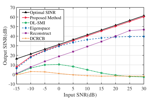
Figure 4: Output SINR versus the input SNR in case of ACP errors for the first scenario.

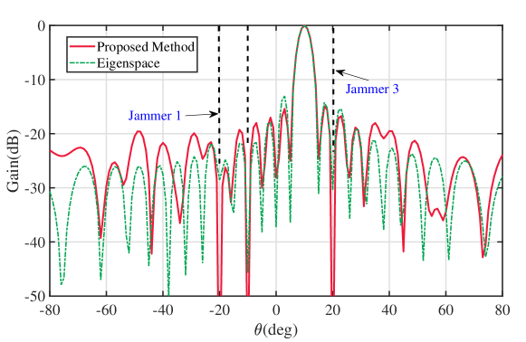
Figure 5: Steady state beampatterns in case of ACP errors for first scenario ( SNR=10dB ).

4.2 Example2: Mismatch due to Looking Direction Error and random ACPs errors with SV perturbation

In the second example, assume that the random direction errors of desired signal and interference are uniformly distributed in $\left[-5{\degree},5{\degree}\right]$ for each simulation, and associated with the random ACP errors of FCA which are uniformly distributed in $\left[-15,15\right]\,mm$ of $\Delta R_{1}$ and $\left[-20,20\right]\,mm$ of $\Delta R_{2}$. Fig.6 shows that the proposed method achieves better performance than others, but there is a 8 dB performance gap between the proposed method and the optimal one. The main reason is the mismatch of the estimated SV with the actual one in the resulting beamformer, which has a slight derivation in this comprehensive case. As a comparation, we compare our method with the Reconstruct method. It is also shown in quiescent beampatterns in Fig.7 that the maximum gain direction (i.e., 0°) deviates from the actual SOI (i.e., 10.5°in this case).

Moreover, Fig.7 shows the ability of the proposed method to have the deepest nulls at the actual interferer DOAs (i.e., 17.8°, -24.1°, -8.9°) which have small deviations from the presumed ones, associated with a wide gain range in the neighbor of the actual SOI direction. In addition, the proposed beamformer exhibits better sidelobe suppression capability than the conventional Reconstruct method in the case of hybrid looking direction error and ACPs errors.

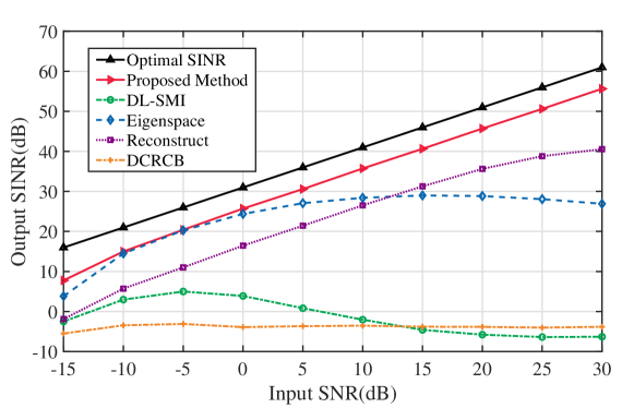
Figure 6: Output SINR versus the input SNR for the second scenario.

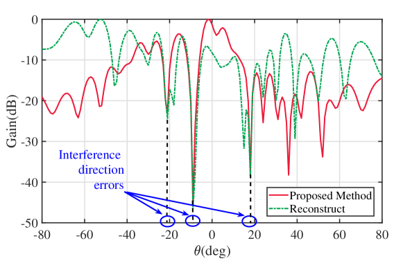
Figure 7: Steady state beampatterns for the second scenario ( SNR=10 dB ).

4.3 Example3:Impacts of mutual coupling effect associated with mixed mismatches

In the above scenarios, the antenna array is assumed to be ideal ($\boldsymbol{C}=\boldsymbol{I}$). However, these assumptions are not fully satisfied in practice due to uncertainties in element position and violation of the isotropic hypothesis. In this example, $\boldsymbol{C}$ is obtained by HFSS. The array configuration for the model in [41] is shown in Fig.8. To examine the effect of mutual coupling for FCA, three element spacing cases ($0.54\lambda,0.5\lambda$ and $0.45\lambda$, corresponding to different $R_{1}$ and $R_{2}$, and simulation of the expansion, initial, and shrinkage state of SWMA) are considered to be associated with ACP errors. The other parameters are the same with example 2. Fig.9 illustrates the performance of competing beamformers with $0.54\lambda,0.5\lambda$ and $0.45\lambda$ element spacing at input SNR=20 dB, respectively.

Some observations are made from the figures:

• The performance of all beamformers is degraded considering mutual coupling effects at lower input SNR.

• The proposed method maintains the output SINR after compensating the mutual coupling effect, which is only reduced by 2 dB compared with Fig.6, while the other methods degrade by 10 dB without considering mutual coupling when input SNR is less than -10 dB. This is due to the radiation energy consumption in the adjacent elements.

• When the spacing between the elements is approximately half of the wavelength, minimal fluctuations in spacing have negligible impact on the resulting SINR, which indicates that variations in mutual coupling between the array elements are also minor. This fact also shows the feasibility of off-line measurement of MCM.

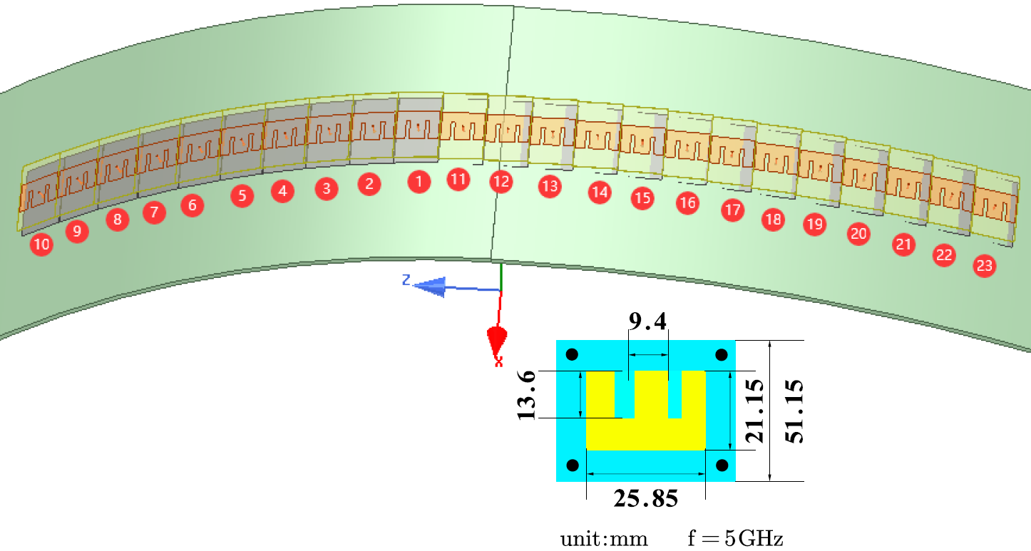
Figure 8: Geometry of a 23-element sectorial FCA (with view of the E-type antenna element on cylindrical surface, a substrate with $\varepsilon_{r}=2.2$ and a thickness of 1.57 mm is used, the work frequency is 5GHz

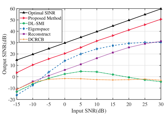
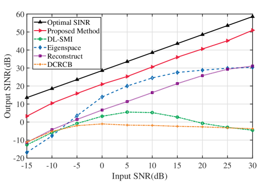
Figure 9: Output SINR versus the input SNR for third scenario, (a) $0.54\lambda$ element spacing, (b) $0.5\lambda$, (c) $0.45\lambda$.

After compensating, our method ensures that the output SNR of the beamformer does not deteriorate with the mutual coupling. Thus, the effectiveness of our proposed method is verified.

5 CONCLUSION

Considering the mutual coupling effect together with mixed mismatches in beamforming for FCA, we propose a robust beamforming algorithm based on multiple domain INCM reconstruction and alternative optimization. We verified from computer simulations that the proposed method outperforms other robust beamformers in respect of SINR output and beam focusing to the target. In the future, we will investigate a more complex situations to reconstruct the optimized object and figure out a simplified algorithm to calculate INCM. Moreover, the proposed algorithms show superior attitude against mutual coupling by introducing mutual coupling matrix into the beamformer while the performance of other robust approaches is unstable. Future work may analyse other scenarios such as near field effect, multiple control parameter FCA, and a theoretical demonstrator.

APPENDIX

5.1 Derivation of (16) and (17)

Considering the structure of the FCA illustrated in Fig.2, the SV of SOI with the mismatch of ACPs can be denoted as

$$\bar{\mathbf{a}}\left(\theta_{1},r_{1},r_{2}\right)=\bar{\mathbf{a}}_{pr}\left(\theta_{1},\bar{r}_{1},\bar{r}_{2}\right)\odot\boldsymbol{\alpha}\left(\theta_{1},x,y\right)$$ (21)

where $\left|x\right|=\left|r_{1}-\bar{r}_{1}\right|,\left|y\right|=\left|r_{2}-\bar{r}_{2}\right|$. $\bar{\mathbf{a}}_{pr}\left(\theta_{1},\bar{r}_{1},\bar{r}_{2}\right)$ is the presumed SV without mismatch of ACPs. $\boldsymbol{\alpha}\left(\theta_{1},x,y\right)$ is the deviation between the real and the assumed SV.

$$\bar{\mathbf{a}}_{pr}= \left[\begin{matrix}e^{jk\boldsymbol{p}_{1}\left(\bar{r}_{1},\bar{r}_{2}\right)\cdot\boldsymbol{u}\left(\theta_{i}\right)}&\cdots&e^{jk\boldsymbol{p}_{S}\left(\bar{r}_{1},\bar{r}_{2}\right)\cdot\boldsymbol{u}\left(\theta_{i}\right)}\\ \end{matrix}\right]^{T}$$ (22)

$$\boldsymbol{\alpha}= \left[\begin{matrix}e^{jk\boldsymbol{p}_{1}\left(x,y\right)\cdot\boldsymbol{u}\left(\theta_{i}\right)}&\cdots&e^{jk\boldsymbol{p}_{S}\left(x,y\right)\cdot\boldsymbol{u}\left(\theta_{i}\right)}\\ \end{matrix}\right]^{T}$$

Then using (21), (17) can be reformulated as

$$p_{2}^{\left(m\right)}:\left\{\begin{array}[]{l}\underset{x,y}{\min}\,\,\,\boldsymbol{\alpha}^{H}\hat{\boldsymbol{R}}_{eq}\boldsymbol{\alpha}+\mathrm{Re}\{(\mathbf{e}_{\bot}^{\left(m\right)})^{H}\grave{\boldsymbol{R}}\mathrm{diag}\left(\bar{\mathbf{a}}_{pr}^{H}\right)\boldsymbol{\alpha}\}\\ s.t.\boldsymbol{\alpha}^{H}\mathrm{diag}\left(\bar{\mathbf{a}}_{pr}^{H}\right)\mathbf{e}_{\bot}^{\left(m\right)}=0,\left|x\right|\leqslant l_{1},\left|y\right|\leqslant l_{2}\\ \end{array}\right.$$ (23)

where we using the following notation

$$\hat{\boldsymbol{R}}_{eq}=\mathrm{diag}\left({\bar{\mathbf{a}}_{pr}}^{H}\right)\boldsymbol{C}^{H}\hat{\boldsymbol{R}}^{-1}\boldsymbol{C}\mathrm{diag}\left(\bar{\mathbf{a}}_{pr}\right)$$ (24)

By virtue of the inner point method, the penalty function $f\left(x,y\right)$ can be represented as (25). Then (23) transformed into the unconstrained optimization problem $\min f\left(x,y\right)$ and Newton’s method can be applied in this case.

$$f\left(x,y\right)= \boldsymbol{\alpha}^{H}\hat{\boldsymbol{R}}_{eq}\boldsymbol{\alpha}+\mathrm{Re}\{(\mathbf{e}_{\bot}^{\left(m\right)})^{H}\grave{\boldsymbol{R}}\mathrm{diag}\left(\bar{\mathbf{a}}^{H}\right)\boldsymbol{\alpha}\}+$$ (25)

$$\epsilon^{\left(k\right)}\boldsymbol{\alpha}^{H}\mathrm{diag}\left(\bar{\mathbf{a}}^{H}\right)\mathbf{e}_{\bot}^{\left(m\right)}(\mathbf{e}_{\bot}^{\left(m\right)})^{H}\mathrm{diag}\left(\bar{\mathbf{a}}\right)\boldsymbol{\alpha}-$$

$$\epsilon^{\left(k\right)}\ln\left(l_{1}^{2}-x^{2}\right)-\epsilon^{\left(k\right)}\ln\left(l_{2}^{2}-y^{2}\right)-$$

$$\epsilon^{\left(k\right)}\ln\mathrm{(}-\mathrm{Re}\{(\mathbf{e}_{\bot}^{\left(m\right)})^{H}\grave{\boldsymbol{R}}\mathrm{diag}\left(\bar{\mathbf{a}}^{H}\right)\boldsymbol{\alpha}\}-(\mathbf{e}_{\bot}^{\left(m\right)})^{H}\grave{\boldsymbol{R}}\mathbf{e}_{\bot}^{\left(m\right)})$$

Here $\epsilon^{\left(k\right)},k=0,1,\cdots$, is a parameter sequence of barrier weight, which satisfies $\epsilon^{\left(k\right)}\rightarrow 0$. We write the first derivative of $f\left(x,y\right)$ in (26) and (27).

$$\frac{\partial f}{\partial x}= \mathrm{Re}\{{\dot{\boldsymbol{\alpha}}_{x}}^{H}\hat{\boldsymbol{R}}_{eq}\boldsymbol{\alpha}\}+\mathrm{Re}\{{\mathbf{e}^{H}}_{\bot}\grave{\boldsymbol{R}}\mathrm{diag}\left(\bar{\mathbf{a}}^{H}\right)\dot{\boldsymbol{\alpha}}_{x}\}+$$ (26)

$$\epsilon^{\left(k\right)}\mathrm{Re}\{{\dot{\boldsymbol{\alpha}}_{x}}^{H}\mathrm{diag}\left(\bar{\mathbf{a}}^{H}\right)\mathbf{e}_{\bot}^{\left(m\right)}(\mathbf{e}_{\bot}^{\left(m\right)})^{H}\mathrm{diag}\left(\bar{\mathbf{a}}\right)\boldsymbol{\alpha}\}+$$

$$\frac{2x}{l_{1}^{2}-x^{2}}\epsilon^{\left(k\right)}-\frac{\mathrm{Re}\{(\mathbf{e}_{\bot}^{\left(m\right)})^{H}\grave{\boldsymbol{R}}\mathrm{diag}\left(\bar{\mathbf{a}}^{H}\right)\dot{\boldsymbol{\alpha}}_{x}\}}{\mathrm{Re}\{(\mathbf{e}_{\bot}^{\left(m\right)})^{H}\grave{\boldsymbol{R}}\mathrm{diag}\left(\bar{\mathbf{a}}^{H}\right)\boldsymbol{\alpha}\}+(\mathbf{e}_{\bot}^{\left(m\right)})^{H}\grave{\boldsymbol{R}}\mathbf{e}_{\bot}^{\left(m\right)}}\epsilon^{\left(k\right)}$$

$$\frac{\partial f}{\partial y}= \mathrm{Re}\{{\dot{\boldsymbol{\alpha}}_{x}}^{H}\hat{\boldsymbol{R}}_{eq}\boldsymbol{\alpha}\}+\mathrm{Re}\{{\mathbf{e}^{H}}_{\bot}\grave{\boldsymbol{R}}\mathrm{diag}\left(\bar{\mathbf{a}}^{H}\right)\dot{\boldsymbol{\alpha}}_{y}\}+$$ (27)

$$\epsilon^{\left(k\right)}\mathrm{Re}\{{\dot{\boldsymbol{\alpha}}_{y}}^{H}\mathrm{diag}\left(\bar{\mathbf{a}}^{H}\right)\mathbf{e}_{\bot}^{\left(m\right)}(\mathbf{e}_{\bot}^{\left(m\right)})^{H}\mathrm{diag}\left(\bar{\mathbf{a}}\right)\boldsymbol{\alpha}\}+$$

$$\frac{2y}{l_{1}^{2}-y^{2}}\epsilon^{\left(k\right)}-\frac{\mathrm{Re}\{(\mathbf{e}_{\bot}^{\left(m\right)})^{H}\grave{\boldsymbol{R}}\mathrm{diag}\left(\bar{\mathbf{a}}^{H}\right)\dot{\boldsymbol{\alpha}}_{y}\}}{\mathrm{Re}\{(\mathbf{e}_{\bot}^{\left(m\right)})^{H}\grave{\boldsymbol{R}}\mathrm{diag}\left(\bar{\mathbf{a}}^{H}\right)\boldsymbol{\alpha}\}+(\mathbf{e}_{\bot}^{\left(m\right)})^{H}\grave{\boldsymbol{R}}\mathbf{e}_{\bot}^{\left(m\right)}}\epsilon^{\left(k\right)}$$

where we use the notation of

$$\dot{\boldsymbol{\alpha}}_{x} =\frac{\partial\boldsymbol{\alpha}\left(x,y\right)}{\partial x}=jk\tilde{\boldsymbol{\mu}}_{\boldsymbol{u}}\odot\boldsymbol{\alpha}$$ (28)

$$\dot{\boldsymbol{\alpha}}_{y} =\frac{\partial\boldsymbol{\alpha}\left(x,y\right)}{\partial y}=jk\tilde{\boldsymbol{\nu}}_{\boldsymbol{u}}\odot\boldsymbol{\alpha}$$

and $\boldsymbol{u}=\left[\begin{matrix}\cos\theta&\sin\theta\\ \end{matrix}\right]^{T}$,

$$\tilde{\boldsymbol{\nu}}_{\boldsymbol{u}}=\left[\begin{matrix}\boldsymbol{\nu}_{1}^{T}\boldsymbol{u}&\cdots&\boldsymbol{\nu}_{S}^{T}\boldsymbol{u}\\ \end{matrix}\right]^{T},\tilde{\boldsymbol{\mu}}_{\boldsymbol{u}}=\left[\begin{matrix}\boldsymbol{\mu}_{1}^{T}\boldsymbol{u}&\cdots&\boldsymbol{\mu}_{S}^{T}\boldsymbol{u}\\ \end{matrix}\right]^{T}$$ (29)

where

$$\boldsymbol{\mu}_{i}^{T}=\left\{\begin{array}[]{l}\left[\begin{matrix}\sin\beta_{i}&\cos\beta_{i}\\ \end{matrix}\right]^{T},i=-1,\cdots,-M\\ \left[\begin{matrix}0&1\\ \end{matrix}\right],i=1,\cdots,N\\ \end{array}\right.$$ (30)

$$\boldsymbol{\nu}_{i}^{T}=\left\{\begin{array}[]{l}\left[\begin{matrix}0&0\\ \end{matrix}\right],i=-1,\cdots,-M\\ \left[\begin{matrix}\sin\beta_{i}&\cos\beta_{i}-1\\ \end{matrix}\right]^{T},i=1,\cdots,N\\ \end{array}\right.$$

According to the general form of Newton’s method [36], the optimal estimated ACP can be obtained by

$$\boldsymbol{p}^{k+1}=\boldsymbol{p}^{k}-\varrho^{k}\left(\nabla^{2}f\left(x,y\right)\right)^{-1}\nabla f\left(x,y\right)$$ (31)

where, $\varrho^{k}$ is the $k$-th step length coefficient of user choice, $k$ denotes iteration times and

$$\boldsymbol{p}^{k}= \left[\begin{matrix}x^{k}&y^{k}\\ \end{matrix}\right]^{T}$$ (32)

$$\nabla f\left(x,y\right)= \left[\begin{matrix}\frac{\partial f\left(x,y\right)}{\partial x}&\frac{\partial f\left(x,y\right)}{\partial y}\\ \end{matrix}\right]^{T}$$ (33)

$$\nabla^{2}f\left(x,y\right)= \left[\begin{matrix}\frac{\partial^{2}f\left(x,y\right)}{\partial x^{2}}&\frac{\partial^{2}f\left(x,y\right)}{\partial x\partial y}\\ \frac{\partial^{2}f\left(x,y\right)}{\partial y\partial x}&\frac{\partial^{2}f\left(x,y\right)}{\partial y^{2}}\\ \end{matrix}\right]$$ (34)

References

- [1] L. CHU, Q. LI, F. GU, X. DU, Y. HE, Y. DENG, Design, modeling, and control of morphing aircraft: A review, Chinese Journal of Aeronautics 35 (5) (2022) 220–246. doi:https://doi.org/10.1016/j.cja.2021.09.013.
- [2] S. Barbarino, O. Bilgen, R. M. Ajaj, M. I. Friswell, D. J. Inman, A review of morphing aircraft, Journal of Intelligent Material Systems and Structures 22 (9) (2011) 823–877. doi:https://doi.org/10.1177/1045389X11414084.
- [3] M. R. M. Hashemi, A. C. Fikes, M. Gal-Katziri, B. Abiri, F. Bohn, A. Safaripour, M. D. Kelzenberg, E. L. Warmann, P. Espinet, N. Vaidya, E. E. Gdoutos, C. Leclerc, F. Royer, S. Pellegrino, H. A. Atwater, A. Hajimiri, A flexible phased array system with low areal mass density, Nature electronics 2 (5) (2019) 195–205.
- [4] D. E. Williams, C. Dorn, S. Pellegrino, A. Hajimiri, Origami-inspired shape-changing phased array, in: 2020 50th European Microwave Conference (EuMC), 2021, pp. 344–347. doi:10.23919/EuMC48046.2021.9338189.
- [5] X. Tian, H. Chen, M.-M. He, W.-Q. Wang, Fast beampattern synthesis algorithm for flexible conformal array, IEEE Signal Processing Letters 29 (2022) 2417–2421. doi:10.1109/LSP.2022.3223804.
- [6] Y. Jia, M. He, K. Huang, W.-Q. Wang, A wide scanning method for a flexible conformal antenna array with mutual coupling effects, in: 2022 IEEE Region 10 Symposium (TENSYMP), 2022, pp. 1–5. doi:10.1109/TENSYMP54529.2022.9864349.
- [7] Y. Song, D. L. Goff, K. Mouthaan, Highly flexible and conformal 2×2 antenna array on rtv silicone for the 2.4 ghz ism band, in: 2020 IEEE International Symposium on Antennas and Propagation and North American Radio Science Meeting, 2020, pp. 671–672. doi:10.1109/IEEECONF35879.2020.9330010.
- [8] B. D. Braaten, S. Roy, S. Nariyal, M. Al Aziz, N. F. Chamberlain, I. Irfanullah, M. T. Reich, D. E. Anagnostou, A self-adapting flexible (selflex) antenna array for changing conformal surface applications, IEEE Transactions on Antennas and Propagation 61 (2) (2013) 655–665. doi:10.1109/TAP.2012.2226227.
- [9] A. C. Fikes, A. Safaripour, F. Bohn, B. Abiri, A. Hajimiri, Flexible, conformal phased arrays with dynamic array shape self-calibration, in: 2019 IEEE MTT-S International Microwave Symposium (IMS), 2019, pp. 1458–1461. doi:10.1109/MWSYM.2019.8701107.
- [10] D. Anagnostou, M. Iskander, Adaptive flexible antenna array system for deformable wing surfaces, in: 2015 IEEE Aerospace Conference, 2015, pp. 1–6. doi:10.1109/AERO.2015.7119183.
- [11] J. Li, Z. Wang, P. Stoica, Robust Capon Beamforming, John Wiley & Sons, Ltd, 2005, Ch. 3, pp. 91–200. doi:https://doi.org/10.1002/0471733482.ch3.
- [12] Y. Yang, X. Xu, H. Yang, W. Li, Robust adaptive beamforming via covariance matrix reconstruction with diagonal loading on interference sources covariance matrix, Digital Signal Processing 136 (2023) 103977. doi:https://doi.org/10.1016/j.dsp.2023.103977.
- [13] Z. Zheng, T. Yang, W.-Q. Wang, H. C. So, Robust adaptive beamforming via simplified interference power estimation, IEEE Transactions on Aerospace and Electronic Systems 55 (6) (2019) 3139–3152. doi:10.1109/TAES.2019.2899796.
- [14] K. Chaudhari, M. Sutaone, P. Bartakke, Adaptive diagonal loading of mvdr beamformer for sustainable performance in noisy conditions, in: 2020 IEEE Region 10 Symposium (TENSYMP), 2020, pp. 1144–1147. doi:10.1109/TENSYMP50017.2020.9230850.
- [15] X. Wang, W. Zheng, L. Guo, Y. Zhang, H. Song, A robust eigenspace-based adaptive beamforming algorithm, in: IET International Radar Conference (IET IRC 2020), Vol. 2020, 2020, pp. 1404–1409. doi:10.1049/icp.2021.0484.
- [16] C.-C. Lee, J.-H. Lee, Eigenspace-based adaptive array beamforming with robust capabilities, IEEE Transactions on Antennas and Propagation 45 (12) (1997) 1711–1716. doi:10.1109/8.650188.
- [17] Z. L. Yu, Z. Gu, J. Zhou, Y. Li, W. Ser, M. H. Er, A robust adaptive beamformer based on worst-case semi-definite programming, IEEE Transactions on Signal Processing 58 (11) (2010) 5914–5919. doi:10.1109/TSP.2010.2058107.
- [18] S. A. Vorobyov, H. Chen, A. B. Gershman, On the relationship between robust minimum variance beamformers with probabilistic and worst-case distortionless response constraints, IEEE Transactions on Signal Processing 56 (11) (2008) 5719–5724. doi:10.1109/TSP.2008.929866.
- [19] Y. Gu, A. Leshem, Robust adaptive beamforming based on interference covariance matrix reconstruction and steering vector estimation, IEEE Transactions on Signal Processing 60 (7) (2012) 3881–3885. doi:10.1109/TSP.2012.2194289.
- [20] Z. Li, Y. Zhang, Q. Ge, Y. Guo, Middle subarray interference covariance matrix reconstruction approach for robust adaptive beamforming with mutual coupling, IEEE Communications Letters 23 (4) (2019) 664–667. doi:10.1109/LCOMM.2019.2899874.
- [21] Z. Liu, S. Zhao, C. Zhang, G. Zhang, Flexible robust adaptive beamforming method with null widening, IEEE Sensors Journal 21 (9) (2021) 10579–10586. doi:10.1109/JSEN.2021.3060510.
- [22] H. Ruan, R. C. de Lamare, Robust adaptive beamforming based on low-rank and cross-correlation techniques, IEEE Transactions on Signal Processing 64 (15) (2016) 3919–3932. doi:10.1109/TSP.2016.2550006.
- [23] S. Vorobyov, A. Gershman, Z.-Q. Luo, Robust adaptive beamforming using worst-case performance optimization: a solution to the signal mismatch problem, IEEE Transactions on Signal Processing 51 (2) (2003) 313–324. doi:10.1109/TSP.2002.806865.
- [24] X. Yang, Y. Li, F. Liu, T. Lan, T. Long, T. K. Sarkar, Robust adaptive beamforming based on covariance matrix reconstruction with annular uncertainty set and vector space projection, IEEE Antennas and Wireless Propagation Letters 20 (2) (2021) 130–134. doi:10.1109/LAWP.2020.3035232.
- [25] P. Chen, J. Gao, W. Wang, Linear prediction-based covariance matrix reconstruction for robust adaptive beamforming, IEEE Signal Processing Letters 28 (2021) 1848–1852. doi:10.1109/LSP.2021.3111582.
- [26] A. Elnashar, S. M. Elnoubi, H. A. El-Mikati, Further study on robust adaptive beamforming with optimum diagonal loading, IEEE Transactions on Antennas and Propagation 54 (12) (2006) 3647–3658. doi:10.1109/TAP.2006.886473.
- [27] M. Wang, Z. Wang, Z. Cheng, Joint calibration of mutual coupling and channel gain/phase inconsistency using a near-field auxiliary source, in: 2016 IEEE 13th International Conference on Signal Processing (ICSP), 2016, pp. 394–398. doi:10.1109/ICSP.2016.7877862.
- [28] H. Steyskal, J. Herd, Mutual coupling compensation in small array antennas, IEEE Transactions on Antennas and Propagation 38 (12) (1990) 1971–1975. doi:10.1109/8.60990.
- [29] B. C. Ng, C. M. S. See, Sensor-array calibration using a maximum-likelihood approach, IEEE Transactions on Antennas and Propagation 44 (6) (1996) 827–835. doi:10.1109/8.509886.
- [30] R. Lorenz, S. Boyd, Robust minimum variance beamforming, IEEE Transactions on Signal Processing 53 (5) (2005) 1684–1696. doi:10.1109/TSP.2005.845436.
- [31] A. Hassanien, S. A. Vorobyov, K. M. Wong, Robust adaptive beamforming using sequential quadratic programming: An iterative solution to the mismatch problem, IEEE Signal Processing Letters 15 (2008) 733–736. doi:10.1109/LSP.2008.2001115.
- [32] Y. Feng, G. Liao, J. Xu, S. Zhu, C. Zeng, Robust beamforming using multiple constraints relaxation, in: 2018 IEEE 10th Sensor Array and Multichannel Signal Processing Workshop (SAM), 2018, pp. 514–518. doi:10.1109/SAM.2018.8448458.
- [33] L. Huang, J. Zhang, X. Xu, Z. Ye, Robust adaptive beamforming with a novel interference-plus-noise covariance matrix reconstruction method, IEEE Transactions on Signal Processing 63 (7) (2015) 1643–1650. doi:10.1109/TSP.2015.2396002.
- [34] S. Boyd, N. Parikh, E. Chu, B. Peleato, J. Eckstein, 2011. doi:10.1561/2200000016.
- [35] M. Grant, S. Boyd, CVX: Matlab software for disciplined convex programming, version 2.1, http://cvxr.com/cvx (Mar. 2014).
- [36] H. W. Kuhn, A. W. Tucker, Nonlinear Programming, Springer Basel, Basel, 2014.
- [37] B. Friedlander, A. Weiss, Direction finding in the presence of mutual coupling, IEEE Transactions on Antennas and Propagation 39 (3) (1991) 273–284. doi:10.1109/8.76322.
- [38] D. Kelley, Relationships between active element patterns and mutual impedance matrices in phased array antennas, in: IEEE Antennas and Propagation Society International Symposium (IEEE Cat. No.02CH37313), Vol. 1, 2002, pp. 524–527 vol.1. doi:10.1109/APS.2002.1016399.
- [39] Y. Zhang, A. Ghazal, C.-X. Wang, H. Zhou, W. Duan, E.-H. M. Aggoune, Accuracy-complexity tradeoff analysis and complexity reduction methods for non-stationary imt-a mimo channel models, IEEE Access 7 (2019) 178047–178062. doi:10.1109/ACCESS.2019.2957820.
- [40] K.-Y. Wang, A. M.-C. So, T.-H. Chang, W.-K. Ma, C.-Y. Chi, Outage constrained robust transmit optimization for multiuser miso downlinks: Tractable approximations by conic optimization, IEEE Transactions on Signal Processing 62 (21) (2014) 5690–5705. doi:10.1109/TSP.2014.2354312.
- [41] Y. Liu, J. Bai, K. D. Xu, Z. Xu, F. Han, Q. H. Liu, Y. Jay Guo, Linearly polarized shaped power pattern synthesis with sidelobe and cross-polarization control by using semidefinite relaxation, IEEE Transactions on Antennas and Propagation 66 (6) (2018) 3207–3212. doi:10.1109/TAP.2018.2816782.