Entropy change due to stochastic state transitions of odd Langevin system

Abstract

Active microscopic objects, e.g., an enzyme molecule, are modeled by the odd Langevin system, in which energy injection from the substrate to the enzyme is described by the antisymmetric part of the elastic matrix. By applying the Onsager–Machlup integral and large deviation theory to the odd Langevin system, we can calculate the cumulant generating function of the entropy change of a thermal bath due to the state transition. For an $N$-component system, we obtain a formal expression of the cumulant generating function and demonstrate that the oddness $\lambda$, which quantifies the antisymmetric part of the elastic matrix, leads to higher-order cumulants that do not appear in a passive elastic system. To demonstrate the effect of the oddness under the concrete parameter, we analyze the simplest two-component system and obtain the optimal transition path and cumulant generating function. The cumulants obtained from expansion of the cumulant generating function increase monotonically with the oddness. This implies that the oddness causes the uncertainty of stochastic state transitions.

I Introduction

In active matter, e.g., birds, bacteria convert chemical energy into mechanical work. To describe this energy injection by the material constants, odd elasticity, i.e., an antisymmetric part of an elastic tensor, is introduced Scheibner20 ; Fruchart22 . The odd elasticity breaks the Maxwell–Betti reciprocity, which holds on the elastic body conserving the mechanical energy. In other words, the odd elasticity quantifies the energy injection. Originally, odd elasticity was introduced for two-dimensional isotropic solids Scheibner20 and was then extended to plates of moderate thickness Fossati22 , a deformable membrane AlIzzi23 , and linkage systems with active hinges Ishimoto22 ; Brandenbourger22 . Currently, odd elasticity is applied to several biological systems, e.g., starfish embryos Tan22 , human sperm Ishimoto23 , and muscles Shankar22 , to capture their activity. In addition, odd elasticity is implemented programmatically in artificial robots Brandenbourger22 .

Odd elasticity has the potential to describe the structural dynamics of active enzymes, which change their structure during catalytic reactions from the substrate to products or nonreactive binding with inhibiting molecules Togashi10 ; Toyabe15 ; Dey16 ; Brown20 ; Mugnai20 ; Yasuda21a ; HK22 ; Toyabe10 . In the case of catalytic reactions, energy is injected into the enzymes from the substrate. We suggest that odd elasticity can model this energy injection and propose the odd Langevin system model, which is a Langevin system that includes odd elasticity YIKLSHK22 ; YKLHSK22 ; KYILSHK23 .

The entropy production for various nonequilibrium steady states can be calculated using the stochastic thermodynamics framework Seifert12 . Seifert defined a trajectory-dependent entropy and constructed a general theory, including the fluctuation theorem Seifert05 . The steady-state entropy production of the charged Brownian particle in a magnetic field has been calculated in several studies Aquino10 ; Jayannavar07 ; Saha08 ; Aquino09 . Weiss proposed a general theory of the linear Langevin system and calculated the cumulants of entropy production in the steady-state Weiss07 . In addition, models that are mathematically the same as the odd Langevin system have been employed to demonstrate nonequilibrium thermodynamics Buisson23 ; Chernyak06 ; Turitsyn07 ; Noh13 ; Noh14 . We expect that odd elasticity not only contributes to the entropy production on the nonequilibrium steady-state but also contributes to the entropy change due to state transitions.

Here, we consider the stochastic state transition between the initial and final states $\mathbf{x}^{\mathrm{i}}\to\mathbf{x}^{\mathrm{f}}$ with duration time $t_{\mathrm{f}}$. For example, this transition models the conformation change of an enzyme induced by combining the substrate molecule. To extract the statistical properties of these state transitions, we can use the path integral formalism of a stochastic system called the Onsager–Machlup theory Onsager53 ; Tomita74b ; RiskenBook ; ZuckermanBook ; Doi19 ; Wang21 ; FK82 ; TW80 ; Taniguchi07 ; Taniguchi08 . In this theory, the probability of observing each trajectory is given with a quantity referred to as the Onsager–Machlup integral and is used to extract the most probable path Durr ; Wissel79 ; Faccioli06 ; Adib08 ; Wang10 ; Gladrow ; YKLHSK22 . Note that the most probable path of the active particles has attracted significant interest recently Teeffelen08 ; Woillez19 ; Majumdar20 ; Gu20 ; Yasuda22b . This optimization problem is also used to calculate the cumulant generating functions in the framework of the large deviation theory Touchette09 ; Krapivsky14 ; Mallick22 ; Falasco23 . In this paper, we calculate the cumulant generating functions of the entropy changes of a thermal bath due to the state transition $\mathbf{x}^{\mathrm{i}}\to\mathbf{x}^{\mathrm{f}}$ of the odd Langevin system. To perform this calculation, we apply the Onsager–Machlup theory to the $N$-component odd Langevin system. In addition, by solving the optimization program of the Onsager–Machlup integral under the large deviation theory and Varadhan’s theorem Varadhan66 ; Touchette09 , we obtain a formal expression of the cumulant generating functions of the entropy changes. As a result, we found that the odd elasticity leads to the variance of entropy changes, which disappear in the case of a purely passive system. In addition, we perform a specific analysis on a two-component system and demonstrate the concrete expression of the optimal trajectories and cumulant generating functions.

The remainder of this paper is organized as follows. In Section II, we present the formalism of the odd Langevin system and the main formal results of the cumulant generating function of the entropy change by the states transition. Section III calculates the cumulant generating function in the simplest two-component system to demonstrate the drastic influence of oddness on the entropy change. Finally, Section IV provides a summary and relevant discussions.

II Odd Langevin system

Recently, we introduced the odd Langevin system YKLHSK22 ; YIKLSHK22 , which is the stochastic dynamics including odd quantities, e.g., odd elasticity, and we argued the correspondence with conformational dynamics of the catalytic enzyme, which energy is injected into by chemical reactions (Fig. 1 (a)) KYILSHK23 . In the following, we describe the formalism of the $N$-component odd Langevin system and calculate the cumulant generating functions of the entropy changes.

II.1 $N$-component odd Langevin system

Here, we consider the $N$-element vector $\mathbf{x}$ whose components are $x_{i}~{}(i=1,2\cdots N)$, which obey following odd Langevin system YKLHSK22 ; YIKLSHK22 ; KYILSHK23 :

$$\dot{\mathbf{x}}=-\ell k\mathbb{L}\mathbb{K}\mathbf{x}+\mathbb{F}\mathbf{y}(t),$$ (1)

where the dot represents the time derivative, $\dot{\mathbf{x}}=d\mathbf{x}/dt$. Here, $\ell$ is a scalar with a mobility dimension, and $\mathbb{L}$ is an $N\times N$ nondimensional mobility matrix. According to Onsager’s reciprocal theorem and the second law of thermodynamics, $\mathbb{L}$ is a symmetric-positive definite matrix KuboBook ; DoiBook . In addition, $k$ is a scalar having the dimension of a spring constant, $\mathbb{K}$ is an $N\times N$ nondimensional elastic matrix that can be constructed by symmetric and antisymmetric parts YKLHSK22 ; YIKLSHK22 ; KYILSHK23 , i.e., $\mathbb{K}=\mathbb{S}+\lambda\mathbb{A}$, where $\mathbb{S}^{\mathrm{T}}=\mathbb{S}$, $\mathbb{A}^{\mathrm{T}}=-\mathbb{A}$, and the superscript $\mathrm{T}$ represents transpose. $\lambda$ is a scalar representing the magnitude of the antisymmetric part, which can be referred to as “oddness.” For the stability of this system, $\mathbb{K}$ is assumed to be positive definite. The second term on the right-hand side of Eq. (1) represents thermal fluctuations characterized by Gaussian white noise $\mathbf{y}$ satisfying $\langle\mathbf{y}(t)\rangle=0$ and $\langle\mathbf{y}(t)\mathbf{y}(0)\rangle=\mathbb{I}_{N}\delta(t)$, where $\langle\cdot\rangle$ indicates the statistical average, $\mathbb{I}_{N}$ is an $N\times N$ identity matrix, and $\delta(t)$ is Dirac’s delta function. Note that the $N\times N$ amplitude matrix $\mathbb{F}$ obeys the fluctuation-dissipation relation KuboBook ; DoiBook $\mathbb{F}^{\mathrm{T}}\mathbb{F}=2k_{\mathrm{B}}T\ell\mathbb{L}$, where $k_{\mathrm{B}}$ is the Boltzmann constant, $T$ is the temperature of the thermal bath. The relaxation rate of this system is given as $\gamma=\ell k$.

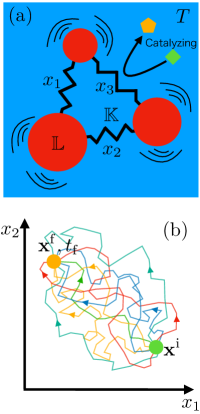
Figure 1: (a) Sketch of an object described by the odd Langevin system Eq. (1) YKLHSK22 ; YIKLSHK22 . The object consists of domains (red circles) connected by springs embedded in the dissipative environment, e.g., a viscous fluid, with temperature $T$. The structure of the object is represented by the set of the spring lengths $\mathbf{x}=(x_{1},x_{2},\cdots,x_{N})^{\mathrm{T}}$. The mobility of the domains is characterized by the mobility matrix $\mathbb{L}$, and the stiffness of springs is characterized by the elastic matrix $\mathbb{K}$. The object catalyzes a chemical reaction from a substrate molecule (green square) to a product molecule (orange pentagon). The energy the object receives from the substrate molecule through the reaction is modeled by the odd elasticity $\lambda\mathbb{A}$. The domains experience fluctuation caused by the thermal noise of the dissipative environment. (b) Stochastic transitions from the initial state $\mathbf{x}^{\mathrm{i}}$ (green circle) to final state $\mathbf{x}^{\mathrm{f}}$ (orange circle) with duration time $t_{\mathrm{f}}$ in a two-dimensional state space. Each trial represented by the trajectories connecting $\mathbf{x}^{\mathrm{i}}$ and $\mathbf{x}^{\mathrm{f}}$ is random and differs from the other trials.

The path probability of the trajectory obeying Eq. (1), $\mathbf{x}(t)$, which begins at $\mathbf{x}^{\mathrm{i}}$ until $t=t_{\mathrm{f}}$, is given as follows Onsager53 ; RiskenBook :

$$P[\mathbf{x}(t)|\mathbf{x}^{\mathrm{i}}]=\mathcal{N}\exp[-O/(2k_{\mathrm{B}}T)].$$ (2)

Here, $O$ is the Onsager–Machlup integral given by YKLHSK22 ; Tomita74b :

$$O=\frac{k}{2}\int_{0}^{t_{\mathrm{f}}}dt\gamma\,[\mathbf{v}\gamma^{-1}+\mathbb{L}\mathbb{K}\mathbf{x}]^{\mathrm{T}}\mathbb{L}^{-1}[\mathbf{v}\gamma^{-1}+\mathbb{L}\mathbb{K}\mathbf{x}],$$ (3)

where $\mathbf{v}=\dot{\mathbf{x}}$, and $\mathcal{N}$ is a normalizing constant.

II.2 Entropy change due to state transitions and its cumulant generating function

Here, we consider the stochastic transitions from the initial state $\mathbf{x}^{\mathrm{i}}$ to the final state $\mathbf{x}^{\mathrm{f}}$ with duration time $t_{\mathrm{f}}$. As shown in Fig. 1(b), the trajectory connecting $\mathbf{x}^{\mathrm{i}}$ and $\mathbf{x}^{\mathrm{f}}$ is independent in each trial because overall the system is stochastic. To characterize the transition $\mathbf{x}^{\mathrm{i}}\to\mathbf{x}^{\mathrm{f}}$, we consider the entropy change of the thermal bath, which quantifies the irreversibility of this transition. Generally, the entropy change depends on $\mathbf{x}^{\mathrm{i}}$ and $\mathbf{x}^{\mathrm{f}}$, as well as the trajectory $\mathbf{x}(t)$ during the transition. In the stochastic thermodynamics framework, the definition of the entropy change $\Delta s$ along trajectory $\mathbf{x}(t)$ is given as $\Delta s:=k_{\mathrm{B}}\ln(P[\mathbf{x}(t)|\mathbf{x}^{\mathrm{i}}]/P[\mathbf{x}^{\mathrm{rev}}(t)|\mathbf{x}^{\mathrm{f}}])$ Seifert12 , where we introduce the reversed trajectory $\mathbf{x}^{\mathrm{rev}}(t)=\mathbf{x}(t_{\mathrm{f}}-t)$. Using Eq. (3), the entropy change $\Delta s$ of the odd Langevin system is given as follows:

$$T\Delta s=-k\int_{0}^{t_{\mathrm{f}}}dt\mathbf{v}^{\mathrm{T}}\mathbb{K}\mathbf{x}.$$ (4)

To characterize the stochastic property of the entropy change, we introduce the cumulant generating function $Q(q):=\ln\langle e^{q\Delta s/k_{\mathrm{B}}}\rangle_{\mathrm{i}\to\mathrm{f}}$ KardarBook , where $\langle\circ\rangle_{\mathrm{i}\to\mathrm{f}}$ indicates the statistical average under the condition of the initial and final state:

$$\langle\circ\rangle_{\mathrm{i}\to\mathrm{f}}:=\int_{\mathbf{x}^{\mathrm{i}}}^{\mathbf{x}^{\mathrm{f}}}\mathcal{D}\mathbf{x}\,\circ P[\mathbf{x}(t)|\mathbf{x}^{\mathrm{i}},\mathbf{x}^{\mathrm{f}}].$$ (5)

Here, $P[\mathbf{x}(t)|\mathbf{x}^{\mathrm{i}},\mathbf{x}^{\mathrm{f}}]$ is a path probability under the condition that $\mathbf{x}(0)=\mathbf{x}^{\mathrm{i}}$ and $\mathbf{x}(t_{\mathrm{f}})=\mathbf{x}^{\mathrm{f}}$, and can be given by Bayes’ theorem $P[\mathbf{x}(t)|\mathbf{x}^{\mathrm{i}},\mathbf{x}^{\mathrm{f}}]\mathcal{P}(\mathbf{x}^{\mathrm{f}}|\mathbf{x}^{\mathrm{i}})=P[\mathbf{x}(t)|\mathbf{x}^{\mathrm{i}}]$, where $\mathcal{P}(\mathbf{x}^{\mathrm{f}}|\mathbf{x}^{\mathrm{i}})$ is a probability of $\mathbf{x}^{\mathrm{f}}$ at $t_{\mathrm{f}}$ under the condition $\mathbf{x}(0)=\mathbf{x}^{\mathrm{i}}$. In addition, $\int_{\mathbf{x}^{\mathrm{i}}}^{\mathbf{x}^{\mathrm{f}}}\mathcal{D}\mathbf{x}$ indicates the path integral over all trajectories $\mathbf{x}(t)$ satisfying $\mathbf{x}(0)=\mathbf{x}^{\mathrm{i}}$ and $\mathbf{x}(t_{\mathrm{f}})=\mathbf{x}^{\mathrm{f}}$. According to Eq. (2), the cumulant generating function of the entropy change is rewritten as follows:

$$Q(q)=C+\ln\int_{\mathbf{x}^{\mathrm{i}}}^{\mathbf{x}^{\mathrm{f}}}\mathcal{D}\mathbf{x}\exp[-\hat{O}/(2k_{\mathrm{B}}T)],$$ (6)

where $C$ is a $q$-independent constant determined by a normalization condition $Q(0)=0$, and $\hat{O}$ is the modified Onsager–Machlup integral:

$$\hat{O}:=O-2qT\Delta s$$

$$=(1+2q)\Delta U+\frac{k}{2}\int_{0}^{t_{\mathrm{f}}}dt\gamma\,\begin{pmatrix}\mathbf{x}\\ \mathbf{v}\gamma^{-1}\end{pmatrix}^{\mathrm{T}}(\mathbb{R}_{0}+q\lambda\mathbb{R}_{1})\begin{pmatrix}\mathbf{x}\\ \mathbf{v}\gamma^{-1}\end{pmatrix}.$$ (7)

Here, $\Delta U$ represents the difference of elastic energy between the initial and final states:

$$\Delta U:=\frac{k}{2}[(\mathbf{x}^{\mathrm{f}})^{\mathrm{T}}\mathbb{S}\mathbf{x}^{\mathrm{f}}-(\mathbf{x}^{\mathrm{i}})^{\mathrm{T}}\mathbb{S}\mathbf{x}^{\mathrm{i}}],$$ (8)

including only the symmetric part of the elastic matrix $\mathbb{S}$. In addition, the following $2N\times 2N$ matrixes are introduced:

$$\mathbb{R}_{0}:=\begin{pmatrix}\mathbb{K}^{\mathrm{T}}\mathbb{L}\mathbb{K}&-\lambda\mathbb{A}\\ \lambda\mathbb{A}&\mathbb{L}^{-1}\end{pmatrix},~{}~{}~{}\mathbb{R}_{1}:=\begin{pmatrix}\mathbb{O}_{N}&-2\mathbb{A}\\ 2\mathbb{A}&\mathbb{O}_{N}\end{pmatrix},$$ (9)

where $\mathbb{O}_{N}$ is an $N\times N$ zero matrix. Note that all cumulants $\langle\Delta s^{n}\rangle_{\mathrm{c}}$ are obtained from $Q(q)$ as KardarBook :

$$\langle\Delta s^{n}\rangle_{\mathrm{c}}=k_{\mathrm{B}}^{n}\left.\frac{d^{n}}{dq^{n}}Q(q)\right|_{q=0}.$$ (10)

Under the large deviation theory and Varadhan’s theorem Varadhan66 ; Touchette09 , the cumulant generating function is approximated as follows:

$$Q(q)-C\sim-\inf_{\mathbf{x}(t)|\mathbf{x}^{\mathrm{i}},\mathbf{x}^{\mathrm{f}}}[\hat{O}]/(2k_{\mathrm{B}}T).$$ (11)

This means that we can calculate the cumulant generating function by considering the optimization problem of $\hat{O}$ with respect to the trajectory $\mathbf{x}(t)$ under the condition that $\mathbf{x}(0)=\mathbf{x}^{\mathrm{i}}$ and $\mathbf{x}(t_{\mathrm{f}})=\mathbf{x}^{\mathrm{f}}$.

In this study, we found that the cumulant generating function of the entropy change due to state transition $\mathbf{x}^{\mathrm{i}}\to\mathbf{x}^{\mathrm{f}}$ with duration time $t_{\mathrm{f}}$ is given in the following form:

$$Q(q)=-\frac{q\Delta U}{k_{\mathrm{B}}T}-\frac{k}{2k_{\mathrm{B}}T}\sum_{n=1}\frac{q^{n}\lambda^{n}}{2}\begin{pmatrix}\mathbf{x}^{\mathrm{i}}\\ \mathbf{x}^{\mathrm{f}}\end{pmatrix}^{\mathrm{T}}\mathbb{E}_{n}(\lambda,t_{\mathrm{f}})\begin{pmatrix}\mathbf{x}^{\mathrm{i}}\\ \mathbf{x}^{\mathrm{f}}\end{pmatrix},$$ (12)

where $\mathbb{E}_{n}$ are $2N\times 2N$ matrixes that characterize each cumulants. Note that the formal expression of $\mathbb{E}_{n}$ is given in Eq. (33). From this expression, we find that the oddness $\lambda$ contributes to the first cumulant and higher cumulants, which implies that the oddness leads to an uncertainty of the entropy change due to transitions. In contrast, if the elastic matrix is symmetric ($\lambda=0$), we can obtain the cumulant generating function from Eq. (12) as follows:

$$Q(q)=-q\frac{\Delta U}{k_{\mathrm{B}}T}.$$ (13)

Thus, the first cumulant and higher cumulants are given as:

$$\langle\Delta s\rangle_{\mathrm{c}}=-\frac{\Delta U}{T},$$ (14)

$$\langle\Delta s^{2}\rangle_{\mathrm{c}}=\langle\Delta s^{3}\rangle_{\mathrm{c}}=\cdots=0.$$ (15)

This means that the entropy change corresponds to elastic energy change between the initial and final state without error, and this is compatible with thermodynamics. The thermodynamic first law of the system without mechanical work is $\Delta U=-Q$, and the entropy change of the thermal bath is related to the heat $Q$ transferred from the system to the bath, i.e., $\Delta s=Q/T$.

II.3 Extremum equation and its solutions

In the following, we present the derivation of Eq. (12) and a formal expression for the matrix $\mathbb{E}_{n}$. Recalling Eq. (11), we consider the variational problem of $\hat{O}$, i.e., $\delta\hat{O}=0$ Touchette09 ; Durr ; YKLHSK22 to obtain $\inf_{\mathbf{x}}[\hat{O}]$. This requirement and Eq. (7) lead to the following extremum equation:

$$\dot{\mathbf{v}}\gamma^{-2}+2(1+2q)\lambda\mathbb{L}\mathbb{A}\mathbf{v}\gamma^{-1}-\mathbb{L}\mathbb{K}^{\mathrm{T}}\mathbb{L}\mathbb{K}\mathbf{x}=0.$$ (16)

This equation can be rewritten as follows:

$$\begin{pmatrix}\dot{\mathbf{x}}\gamma^{-1}\\ \dot{\mathbf{v}}\gamma^{-2}\end{pmatrix}=\mathbb{G}\begin{pmatrix}\mathbf{x}\\ \mathbf{v}\gamma^{-1}\end{pmatrix},$$ (17)

where $\mathbb{G}$ is a $2N\times 2N$ matrix given as:

$$\mathbb{G}:=\begin{pmatrix}\mathbb{O}_{N}&\mathbb{I}_{N}\\ \mathbb{L}\mathbb{K}^{\mathrm{T}}\mathbb{L}\mathbb{K}&-2(1+2q)\lambda\mathbb{L}\mathbb{A}\end{pmatrix}.$$ (18)

To obtain the cumulants in order, we expand the variables as $\mathbf{x}=\sum_{n}q^{n}\mathbf{x}_{n},\mathbf{v}=\sum_{n}q^{n}\mathbf{v}_{n}$ and obtain the equation for each component from Eq. (17) as follows:

$$\begin{pmatrix}\dot{\mathbf{x}}_{n}\gamma^{-1}\\ \dot{\mathbf{v}}_{n}\gamma^{-2}\end{pmatrix}=\mathbb{G}_{0}\begin{pmatrix}\mathbf{x}_{n}\\ \mathbf{v}_{n}\gamma^{-1}\end{pmatrix}+\lambda\mathbb{G}_{1}\begin{pmatrix}\mathbf{x}_{n-1}\\ \mathbf{v}_{n-1}\gamma^{-1}\end{pmatrix},$$ (19)

where we use the following $2N\times 2N$ matrixes:

$$\mathbb{G}_{0}:=\begin{pmatrix}\mathbb{O}_{N}&\mathbb{I}_{N}\\ \mathbb{L}\mathbb{K}^{\mathrm{T}}\mathbb{L}\mathbb{K}&-2\lambda\mathbb{L}\mathbb{A}\end{pmatrix},~{}\mathbb{G}_{1}:=\begin{pmatrix}\mathbb{O}_{N}&\mathbb{O}_{N}\\ \mathbb{O}_{N}&-4\mathbb{L}\mathbb{A}\end{pmatrix}.$$ (20)

For $n=0$, we obtain the following formal solution to Eq. (19) with a matrix exponential:

$$\begin{pmatrix}\mathbf{x}_{0}\\ \mathbf{v}_{0}\gamma^{-1}\end{pmatrix}=e^{\mathbb{G}_{0}\tau}\begin{pmatrix}\mathbf{c}_{0}\\ \mathbf{d}_{0}\end{pmatrix},$$ (21)

where $\tau=t\gamma$ is a dimensionless time, and $\mathbf{c}_{0}$ and $\mathbf{d}_{0}$ are constants determined with the boundary conditions, i.e., $\mathbf{x}_{0}(0)=\mathbf{x}^{\mathrm{i}}$ and $\mathbf{x}_{0}(t_{\mathrm{f}})=\mathbf{x}^{\mathrm{f}}$. These boundary conditions can be rewritten in the following form:

$$\begin{pmatrix}\mathbf{x}^{\mathrm{i}}\\ 0\\ \mathbf{x}^{\mathrm{f}}\\ 0\end{pmatrix}=\mathbb{B}\begin{pmatrix}\mathbf{c}_{0}\\ \mathbf{d}_{0}\\ \mathbf{v}^{\mathrm{i}}\gamma^{-1}\\ \mathbf{v}^{\mathrm{f}}\gamma^{-1}\end{pmatrix},$$ (22)

where $\mathbf{v}^{\mathrm{i}}=\mathbf{v}_{0}(0)$ and $\mathbf{v}^{\mathrm{f}}=\mathbf{v}_{0}(t_{\mathrm{f}})$ are also constants determined by the above boundary conditions, and $\mathbb{B}$ is a $4N\times 4N$ matrix given as follows:

$$\mathbb{B}:=\begin{pmatrix}\mathbb{I}_{2N}&\mathbb{J}\\ e^{\mathbb{G}_{0}\tau_{\mathrm{f}}}&\mathbb{J}^{\prime}\end{pmatrix},~{}\mathbb{J}:=\begin{pmatrix}\mathbb{O}_{N}&\mathbb{O}_{N}\\ -\mathbb{I}_{N}&\mathbb{O}_{N}\end{pmatrix},~{}\mathbb{J}^{\prime}:=\begin{pmatrix}\mathbb{O}_{N}&\mathbb{O}_{N}\\ \mathbb{O}_{N}&-\mathbb{I}_{N}\end{pmatrix}.$$ (23)

By solving Eq. (22) for $\mathbf{c}_{0}$, $\mathbf{d}_{0}$, $\mathbf{v}^{\mathrm{i}}$, and $\mathbf{v}^{\mathrm{f}}$, we obtain the following:

$$\begin{pmatrix}\mathbf{c}_{0}\\ \mathbf{d}_{0}\\ \mathbf{v}^{\mathrm{i}}\gamma^{-1}\\ \mathbf{v}^{\mathrm{f}}\gamma^{-1}\end{pmatrix}=\mathbb{B}^{-1}\begin{pmatrix}\mathbf{x}^{\mathrm{i}}\\ 0\\ \mathbf{x}^{\mathrm{f}}\\ 0\end{pmatrix},~{}~{}~{}\begin{pmatrix}\mathbf{c}_{0}\\ \mathbf{d}_{0}\end{pmatrix}=\hat{\mathbb{B}}^{-1}\begin{pmatrix}\mathbf{x}^{\mathrm{i}}\\ \mathbf{x}^{\mathrm{f}}\end{pmatrix}.$$ (24)

Here, $\hat{\mathbb{B}}^{-1}$ is a $2N\times 2N$ matrix comprising $2N\times N$ matrixes $\mathbb{C}_{n}$, which are the block matrixes of $\mathbb{B}^{-1}$:

$$\mathbb{B}^{-1}=\begin{pmatrix}\mathbb{C}_{1}&\mathbb{C}_{2}&\mathbb{C}_{3}&\mathbb{C}_{4}\\ \mathbb{C}_{5}&\mathbb{C}_{6}&\mathbb{C}_{7}&\mathbb{C}_{8}\\ \end{pmatrix}.$$ (25)

Using $\mathbb{C}_{n}$, we have $\hat{\mathbb{B}}^{-1}:=\begin{pmatrix}\mathbb{C}_{1}&\mathbb{C}_{3}\end{pmatrix}$, and we use $\tilde{\mathbb{B}}^{-1}:=\begin{pmatrix}\mathbb{C}_{3}&\mathbb{C}_{4}\end{pmatrix}$ later.

For arbitrary $n$, we have the following formal solution to Eq. (19):

$$\begin{pmatrix}\mathbf{x}_{n}\\ \mathbf{v}_{n}\gamma^{-1}\end{pmatrix} =\sum_{m=0}^{n}\left[\lambda^{m}e^{\mathbb{G}_{0}\tau}\mathbb{M}_{m}(\tau)\begin{pmatrix}\mathbf{c}_{n-m}\\ \mathbf{d}_{n-m}\end{pmatrix}\right],$$ (26)

where $\mathbf{c}_{n}$ and $\mathbf{d}_{n}$ are constants determined with the boundary conditions, i.e., $\mathbf{x}_{n}(0)=\mathbf{x}_{n}(t_{\mathrm{f}})=0$. We also used the following functions:

$$\mathbb{M}_{m}(\tau):=\int_{0}^{\tau}d\tau_{1}\mathbb{H}(\tau_{1})\cdots\int_{0}^{\tau_{m-1}}d\tau_{m}\mathbb{H}(\tau_{m}),$$ (27)

$$\mathbb{H}(\tau):=e^{-\mathbb{G}_{0}\tau}\mathbb{G}_{1}e^{\mathbb{G}_{0}\tau}.$$ (28)

Using the boundary conditions, we obtain the following relation (see also App.A):

$$\begin{pmatrix}\mathbf{c}_{n}\\ \mathbf{d}_{n}\end{pmatrix}=\lambda^{n}\mathbb{N}_{n}\begin{pmatrix}\mathbf{c}_{0}\\ \mathbf{d}_{0}\end{pmatrix},$$ (29)

where $\mathbb{N}_{n}$ is a matrix determined by the following recurrence relation:

$$\mathbb{N}_{n}=\sum_{m=1}^{n}-\tilde{\mathbb{B}}^{-1}e^{\mathbb{G}_{0}\tau_{\mathrm{f}}}\mathbb{M}_{m}(\tau_{\mathrm{f}})\mathbb{N}_{n-m}$$ (30)

with $\mathbb{N}_{0}=\mathbb{I}_{2N}$. From Eqs. (26) and (29), the solution satisfying the boundary conditions is given as follows:

$$\begin{pmatrix}\mathbf{x}_{n}\\ \mathbf{v}_{n}\gamma^{-1}\end{pmatrix}=\lambda^{n}e^{\mathbb{G}_{0}\tau}\mathbb{T}_{n}(\tau)\hat{\mathbb{B}}^{-1}\begin{pmatrix}\mathbf{x}^{\mathrm{i}}\\ \mathbf{x}^{\mathrm{f}}\end{pmatrix},$$ (31)

$$\mathbb{T}_{n}(\tau):=\sum_{m=0}^{n}\left[\mathbb{M}_{m}(\tau)\mathbb{N}_{n-m}\right].$$ (32)

By substituting the above solutions into the modified Onsager–Machlup integral Eq. (7) and by comparing with Eq. (12), we obtain the following formal expression of $\mathbb{E}_{n}$:

$$\mathbb{E}_{n}=\hat{\mathbb{B}}^{-1,\mathrm{T}}\sum_{m=0}^{n}\left[\int_{0}^{\tau_{\mathrm{f}}}d\tau\,\mathbb{T}_{m}^{\mathrm{T}}(\tau)e^{\mathbb{G}_{0}^{\mathrm{T}}\tau}\mathbb{R}_{0}e^{\mathbb{G}_{0}\tau}\mathbb{T}_{n-m}(\tau)\right]\hat{\mathbb{B}}^{-1}$$

$$+\hat{\mathbb{B}}^{-1,\mathrm{T}}\sum_{m=0}^{n-1}\left[\int_{0}^{\tau_{\mathrm{f}}}d\tau\,\mathbb{T}_{m}^{\mathrm{T}}(\tau)e^{\mathbb{G}_{0}^{\mathrm{T}}\tau}\mathbb{R}_{1}e^{\mathbb{G}_{0}\tau}\mathbb{T}_{n-m-1}(\tau)\right]\hat{\mathbb{B}}^{-1}.$$ (33)

This expression can be used to calculate the cumulant generating function for a specific parameter set of $\mathbb{L}$ and $\mathbb{K}$. Although the simplest two-component system is discussed in Sec. III, concrete calculations for other systems are left for future work.

III Two-component system

To demonstrate the influence of odd elasticity on the entropy change, we consider a two-component system, i.e., $N=2$, and we calculate the cumulant generating function analytically. We also assume the simplest case, i.e., $\mathbb{L}=\mathbb{I}_{2},\mathbb{S}=\mathbb{I}_{2}$, and

$$\mathbb{A}=\begin{pmatrix}0&1\\ -1&0\end{pmatrix},$$ (34)

which corresponds mathematically to the charged Brownian particle in the magnetic field Aquino10 ; Jayannavar07 ; Saha08 ; Aquino09 .

Then, the extremum equation Eq. (16) is reduced to:

$$\ddot{\mathbf{x}}\gamma^{-2}+2(1+2q)\lambda\mathbb{A}\dot{\mathbf{x}}\gamma^{-1}-(1+\lambda^{2})\mathbf{x}=0,$$ (35)

which we obtain by modulating an existing equation YKLHSK22 with $q$. A solution to this linear equation is given as follows:

$$\mathbf{x}(\tau)=\sum_{n}^{4}c_{n}\mathbf{u}_{n}e^{g_{n}\tau},$$ (36)

where $\mathbf{u}_{n}$ and $g_{n}$ are the corresponding eigenvector and eigenvalue, respectively:

$$\mathbf{u}_{1}=(1,i)^{\mathrm{T}},~{}~{}~{}g_{1}=\sqrt{1-4\lambda^{2}q(1+q)}-i\lambda(1+2q),$$ (37)

$$\mathbf{u}_{2}=\mathbf{u}_{1},~{}~{}~{}g_{2}=-g_{1}^{*},$$ (38)

$$\mathbf{u}_{3}=\mathbf{u}_{1}^{*},~{}~{}~{}g_{3}=g_{1}^{*},$$ (39)

$$\mathbf{u}_{4}=\mathbf{u}_{1}^{*},~{}~{}~{}g_{4}=-g_{1},$$ (40)

where star indicates a complex conjugate. Here, we impose the initial and final conditions for trajectory $\mathbf{x}(\tau)$ as $\mathbf{x}^{\mathrm{i}}$ and $\mathbf{x}^{\mathrm{f}}$. Then, the solution satisfying these conditions is obtained as follows:

$$\mathbf{x}(\tau)=-\frac{\sinh(b(\tau-\tau_{\mathrm{f}}))}{\sinh(b\tau_{\mathrm{f}})}\mathbb{D}^{\mathrm{T}}(\tau)\mathbf{x}^{\mathrm{i}}+\frac{\sinh(b\tau)}{\sinh(b\tau_{\mathrm{f}})}\mathbb{D}^{\mathrm{T}}(\tau-\tau_{\mathrm{f}})\mathbf{x}^{\mathrm{f}},$$ (41)

where we use the following:

$$\mathbb{D}(\tau):=\begin{pmatrix}\cosh(a\tau)&-i\sinh(a\tau)\\ i\sinh(a\tau)&\cosh(a\tau)\end{pmatrix},$$ (42)

and $a:=i\lambda(1+2q),b:=\sqrt{1-4\lambda^{2}q(1+q)}$.

In Fig. 2, we plot the sample trajectories under the conditions $\bar{\mathbf{x}}^{\mathrm{i}}=(1,0)^{\mathrm{T}}$ (green circles) and $\bar{\mathbf{x}}^{\mathrm{f}}=(-1,0)^{\mathrm{T}}$ (orange circles), where we introduce the dimensionless state variables $\bar{\mathbf{x}}=\sqrt{k/k_{\mathrm{B}}T}\mathbf{x}$. Here, we use specific values $\lambda=1$ and (a) $\tau_{\mathrm{f}}=1$ and (b) $\tau_{\mathrm{f}}=5$. We vary $q$, which are shown using different line colors. Eventually, the variations between the black and other lines lead to cumulants.

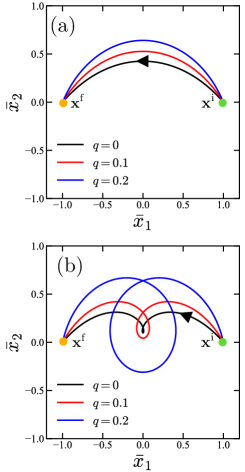
Figure 2: Optimal trajectories for (a) $\tau_{\mathrm{f}}=1$ and (b) $\tau_{\mathrm{f}}=5$ [see Eq. (41)] and $\lambda=1$. The initial and final states are $\bar{\mathbf{x}}^{\mathrm{i}}=\sqrt{k/k_{\mathrm{B}}T}\mathbf{x}^{\mathrm{i}}=(1,0)^{\mathrm{T}}$ (green circles) and $\bar{\mathbf{x}}^{\mathrm{f}}=(-1,0)^{\mathrm{T}}$ (orange circles), respectively. Here, the different colors indicate various $q$ values. The variations between the black ($q=0$) and other lines implies cumulants.

By substituting the solution given by Eq. (41) into Eq. (7), we calculate the cumulant generating function $Q(q)$ as follows:

$$Q(q)=C-\frac{(1+2q)}{2k_{\mathrm{B}}T}\Delta U-\frac{k}{4k_{\mathrm{B}}T}\begin{pmatrix}\mathbf{x}^{\mathrm{i}}\\ \mathbf{x}^{\mathrm{f}}\end{pmatrix}^{\mathrm{T}}\mathbb{E}\begin{pmatrix}\mathbf{x}^{\mathrm{i}}\\ \mathbf{x}^{\mathrm{f}}\end{pmatrix},$$ (43)

where

$$\mathbb{E}=\frac{b}{\sinh(b\tau_{\mathrm{f}})}\begin{pmatrix}\cosh(b\tau_{\mathrm{f}})\mathbb{I}_{2}&-\mathbb{D}(\tau_{\mathrm{f}})\\ -\mathbb{D}^{\mathrm{T}}(\tau_{\mathrm{f}})&\cosh(b\tau_{\mathrm{f}})\mathbb{I}_{2}\end{pmatrix},$$ (44)

and $C$ is a $q$-independent constant determined by an normalization condition $Q(0)=0$. Unlike the formal result given by Eq. (12) in Sec. II, which involves expansion around $q=0$, the result given by Eq. (43) is the full expression for the entire $q$. Notice $\mathbb{E}=\sum_{n=1}q^{n}\lambda^{n}\mathbb{E}_{n}$ for consistency between Eqs. (12) and (43). In Eq. (43), $Q(q;\mathbf{x}^{\mathrm{i}},\mathbf{x}^{\mathrm{f}})=Q(-1-q;\mathbf{x}^{\mathrm{f}},\mathbf{x}^{\mathrm{i}})$, which is known as the Gallavotti–Cohen symmetry Seifert12 equivalent to the fluctuation theorem. We obtain each cumulants by expanding Eq. (43) as Eq. (10). Concrete expressions of the first and second cumulants are given in App. B.

In Fig. 3, we plot the cumulant generating function $Q(q)$, i.e., Eq. (43), under the conditions $\bar{\mathbf{x}}^{\mathrm{i}}=(1,0)^{\mathrm{T}}$ and $\bar{\mathbf{x}}^{\mathrm{f}}=(-1,0)^{\mathrm{T}}$ with $\lambda=1$. Here, the duration time is varied as $\tau_{\mathrm{f}}=1,5$ and $\tau_{\mathrm{f}}\to\infty$, and we show them as a solid black line, a solid red line, and a blue dashed line, respectively. The red solid and blue dashed lines show nearly the same value for the entire $q$. The normalization condition is represented as $Q(0)=0$, which holds in all cases. The slope and curvature at $q=0$ represent the first and second cumulants, respectively.

Considering zero odd elasticity $\lambda=0$, we can confirm that Eq. (43) reduces to Eq. (13), and we can obtain $\langle\Delta s^{1}\rangle_{\mathrm{c}}=-\Delta U/T$ and $\langle\Delta s^{2}\rangle_{\mathrm{c}}=\langle\Delta s^{3}\rangle_{\mathrm{c}}=\cdots=0$, as discussed in Section II for arbitrary $N$.

By taking a long time limit $t_{\mathrm{f}}\to\infty$, we obtain the following:

$$\mathbb{E}=\sqrt{1-4\lambda^{2}q(1+q)}\mathbb{I}_{4}$$ (45)

as a limit of Eq. (44), and the cumulant generating function becomes similar to that for the entropy production of the steady-state transverse diffusion system Buisson23 , which is mathematically the same as the two-component odd Langevin system discussed in this paper. Expanding the long time cumulant generating function (refer to Eqs. (10) and (45)), we obtain the following cumulants up to the fourth order:

$$\langle\Delta s^{1}\rangle_{\mathrm{c}} =-\frac{\Delta U}{T}+\frac{k}{2T}\lambda^{2}[(\mathbf{x}^{\mathrm{i}})^{2}+(\mathbf{x}^{\mathrm{f}})^{2}],$$ (46)

$$\langle\Delta s^{2}\rangle_{\mathrm{c}} =\frac{k_{\mathrm{B}}k}{T}\lambda^{2}(1+\lambda^{2})[(\mathbf{x}^{\mathrm{i}})^{2}+(\mathbf{x}^{\mathrm{f}})^{2}],$$ (47)

$$\langle\Delta s^{3}\rangle_{\mathrm{c}} =\frac{6k_{\mathrm{B}}^{2}k}{T}\lambda^{4}(1+\lambda^{2})[(\mathbf{x}^{\mathrm{i}})^{2}+(\mathbf{x}^{\mathrm{f}})^{2}],$$ (48)

$$\langle\Delta s^{4}\rangle_{\mathrm{c}} =\frac{12k_{\mathrm{B}}^{3}k}{T}\lambda^{4}(1+6\lambda^{2}+5\lambda^{4})[(\mathbf{x}^{\mathrm{i}})^{2}+(\mathbf{x}^{\mathrm{f}})^{2}].$$ (49)

Note that higher cumulants also can be obtained systematically. All cumulants increase monotonically with the oddness $\lambda$, which implies that the uncertainty of the state transition is strengthened by the oddness.

IV Summary and Discussion

In this paper, we have calculated the cumulant generating function of the entropy change of a thermal bath during the state transition $\mathbf{x}^{\mathrm{i}}\to\mathbf{x}^{\mathrm{f}}$ of the odd Langevin system using the path probability determined by the Onsager–Machlup integral and the framework of the large deviation theory. As a result, for the $N$-component system, we have provided a formal expression of the cumulant generating function in Eq. (12), which indicates that the oddness leads to a higher-order cumulant unlike a passive elastic system, where the entropy change is determined by the energy change of the system without error.

To demonstrate the effect of oddness using the concrete parameter setup, we further calculated the cumulant generating function of a simple two-component system. Here, we found that the cumulants increases monotonically with oddness $\lambda$, which implies that the oddness amplifies the uncertainty of the system. The oddness may help us understand the uncertainty of various biological systems, e.g., random responses to stimulations.

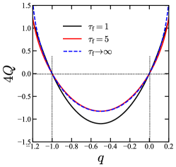
Figure 3: Cumulant generating function (Eq. (43)) for $\lambda=1$. The initial and final states are $\bar{\mathbf{x}}^{\mathrm{i}}=(1,0)^{\mathrm{T}}$ and $\bar{\mathbf{x}}^{\mathrm{f}}=(-1,0)^{\mathrm{T}}$. We vary the duration time as $\tau_{\mathrm{f}}=1,5$ and $\tau_{\mathrm{f}}\to\infty$, which are shown using solid black, solid red, and dashed blue lines, respectively. Note that the solid red and dashed blue lines nearly coincide. All lines hold the normalization condition $Q(0)=0$. The derivatives at $q=0$ are the corresponding cumulants. $Q(-1)=0$ is shown in all cases and indicates that this transition does not change the system entropy $s_{\mathrm{sys}}$, as discussed in Sec. IV.

In the following, we discuss the connection between our results and stochastic thermodynamics. In addition to the entropy of the thermal bath, we consider the system entropy $s_{\mathrm{sys}}(\mathbf{x})=-k_{\mathrm{B}}\ln\mathcal{P}(\mathbf{x})$, where $\mathcal{P}(\mathbf{x})$ is a steady-state distribution. In the odd Langevin system given by Eq. (1), $\mathcal{P}(\mathbf{x})$ is the Gaussian distribution $\mathcal{P}(\mathbf{x})\sim\exp[-\mathbf{x}^{\mathrm{T}}\mathbb{C}^{-1}\mathbf{x}/2]$, where $\mathbb{C}$ is a covariance matrix obtained by solving the Lyapunov equation $k\mathbb{L}\mathbb{K}\mathbb{C}+k\mathbb{C}\mathbb{K}^{\mathrm{T}}\mathbb{L}=2k_{\mathrm{B}}T\mathbb{L}$ YIKLSHK22 . Note that the cumulant generating function $Q(q)$ and system entropy $s_{\mathrm{sys}}$ are connected as $Q(-1)=\ln\langle e^{-\Delta s/k_{\mathrm{B}}}\rangle_{\mathrm{i}\to\mathrm{f}}=\Delta s_{\mathrm{sys}}/k_{\mathrm{B}}$, which is an alternative form of the Jarzynski equality Seifert12 (the derivation of this equality is given in App. C). Thus, the cumulant generating function has information on both the system and the bath entropy change. In Fig. 3, we observe $Q(-1)=0$, which indicates that the system entropy does not change with this specific transition, i.e., $\Delta s_{\mathrm{sys}}=0$.

In addition, the thermodynamic uncertainty relation (TUR) is discussed in the stochastic thermodynamics framework. By defining the TUR-efficiency for the entropy change as $\eta=2k_{\mathrm{B}}\langle\Delta s\rangle_{\mathrm{c}}/\langle\Delta s^{2}\rangle_{\mathrm{c}}$, we obtain TUR expressed as $\eta\leq 1$ Horowitz17 . Using Eqs. (46) and (47) under the condition $\Delta U=0$, the TUR-efficiency becomes $\eta=1/(1+\lambda^{2})$, which satisfies the TUR entire oddness $\lambda$.

An important application of this research is the conformation change of an enzyme from the open state to closed state binding substrate, which can be considered as the state transition $\mathbf{x}^{\mathrm{i}}\to\mathbf{x}^{\mathrm{f}}$. Note that the thermal cost for this transition is evaluated by the entropy change. The energy injected into the enzyme is part of the chemical potential difference between the substrate and the products, e.g., the chemical potential difference between the ATP and ADP molecule is roughly $20k_{\mathrm{B}}T$ Toyabe10 . Here, we assume that the enzyme receives 10% of the chemical potential difference, i.e., $2k_{\mathrm{B}}T$, during the reaction. In the odd Langevin system, the injected energy is represented by $k\lambda a^{2}$, where $a$ is the size of the object, e.g., $10\mathrm{nm}$ for enzyme molecule. Thus, the odd elasticity can be estimated roughly as $k\lambda\sim 2k_{\mathrm{B}}T/(10\mathrm{nm})^{2}\sim 10^{-4}\mathrm{J/m^{2}}$. The duration time for protein folding is roughly estimated as $t_{\mathrm{f}}\sim 1\mathrm{\mu s}$ Chung12 .

Here, we have discussed enzymes as a physical system, as represented by the odd Langevin system. In addition to this example, the odd Langevin system can be used to describe other nonequilibrium physical systems, e.g., charged Brownian particle in a magnetic field Aquino10 ; Jayannavar07 ; Saha08 ; Aquino09 , the polymer molecule in an external shear flow Turitsyn07 , and the transverse diffusion system Noh13 ; Noh14 ; Buisson23 . A previous study Buisson23 reported the cumulant generating function and rate function of the steady-state entropy production of the transverse diffusion system, which is mathematically the same as two-components odd Langevin system (SectionIII). The obtained cumulant generating function is $Q(q)=1-\sqrt{1-4q(1+q)\lambda^{2}}$ Buisson23 . Although this is similar to our results for the long time limit given by Eq. (45), differing from our results, their results for the steady-state do not include the initial and final states. Note that we consider transitions rather than the steady state considered in the literature Buisson23 .

In this study, we calculated the cumulant generating function of entropy change using the Onsager–Machlup integral. The method of the Onsager–Machlup integral and the large deviation theory have diverse applications. One such application is the calculation of the conditioned distribution $\mathcal{P}(\mathbf{x},t|\mathbf{x}^{\mathrm{i}})$ through the optimal problem of the Onsager–Machlup integral Majumdar20 . Another application is the estimation of the mean passage time, which is an average value of the duration time $\langle t_{\mathrm{f}}\rangle$ Woillez19 . These quantities will be calculated in the odd Langevin system.

K.Y. thanks K. Ishimoto and S. Komura for meaningful discussions. K.Y. acknowledges support by a Grant-in-Aid for JSPS Fellows (Grants No. 22KJ1640) from the JSPS and the Research Institute for Mathematical Sciences, an International Joint Usage/Research Center located in Kyoto University. K.Y. would like to thank Enago (www.enago.jp) for the English language review.

Appendix A Derivation of recurrence relation Eq. (30)

Here, we present the derivation of the recurrence relation given in Eq. (30). Using Eq. (26), the boundary conditions $\mathbf{x}_{n}(0)=\mathbf{x}_{n}(t_{\mathrm{f}})=0$ can be rewritten as follows:

$$\begin{pmatrix}0\\ 0\\ -\sum_{m=1}^{n}\left[\lambda^{m}e^{\mathbb{G}_{0}\tau_{\mathrm{f}}}\mathbb{M}_{m}(\tau_{\mathrm{f}})\begin{pmatrix}\mathbf{c}_{n-m}\\ \mathbf{d}_{n-m}\end{pmatrix}\right]\end{pmatrix}=\mathbb{B}\begin{pmatrix}\mathbf{c}_{n}\\ \mathbf{d}_{n}\\ \mathbf{v}^{\mathrm{i}}\gamma^{-1}\\ \mathbf{v}^{\mathrm{f}}\gamma^{-1}\end{pmatrix}.$$ (50)

By solving this equation, we obtain:

$$\begin{pmatrix}\mathbf{c}_{n}\\ \mathbf{d}_{n}\end{pmatrix}=-\tilde{\mathbb{B}}^{-1}\sum_{m=1}^{n}\left[\lambda^{m}e^{\mathbb{G}_{0}\tau_{\mathrm{f}}}\mathbb{M}_{m}(\tau_{\mathrm{f}})\begin{pmatrix}\mathbf{c}_{n-m}\\ \mathbf{d}_{n-m}\end{pmatrix}\right].$$ (51)

By substituting Eq. (29) into the above equation, we obtain the recurrence relation Eq. (30).

Appendix B First and second cumulants for two-component system

In the following, we present the explicit form of the first and second cumulants for the two-component system. Recalling Eq. (10), the first and second cumulants can be obtained via expansion of the cumulant generating function given in Eq. (43).

Here, the first cumulant is given as follows:

$$\langle\Delta s^{1}\rangle_{\mathrm{c}} =-\frac{\Delta U}{T}-\frac{k\lambda}{4T}\begin{pmatrix}\mathbf{x}^{\mathrm{i}}\\ \mathbf{x}^{\mathrm{f}}\end{pmatrix}^{\mathrm{T}}\begin{pmatrix}\mathbb{E}_{1}^{\mathrm{d}}&\mathbb{E}_{1}^{\mathrm{od}}\\ (\mathbb{E}_{1}^{\mathrm{od}})^{\mathrm{T}}&\mathbb{E}_{1}^{\mathrm{d}}\end{pmatrix}\begin{pmatrix}\mathbf{x}^{\mathrm{i}}\\ \mathbf{x}^{\mathrm{f}}\end{pmatrix},$$ (52)

where we use the following matrixes:

$$\mathbb{E}_{1}^{\mathrm{d}}=\frac{2}{\sinh^{2}(\tau_{\mathrm{f}})}\lambda(\tau_{\mathrm{f}}-\cosh(\tau_{\mathrm{f}})\sinh(\tau_{\mathrm{f}}))\mathbb{I}_{2},$$ (53)

$$\mathbb{E}_{1}^{\mathrm{od}}=\frac{2}{\sinh^{2}(\tau_{\mathrm{f}})}[-\lambda(\tau_{\mathrm{f}}\cosh(\tau_{\mathrm{f}})-\sinh(\tau_{\mathrm{f}}))\mathbb{D}_{0}$$

$$+\tau_{\mathrm{f}}\sinh(\tau_{\mathrm{f}})\hat{\mathbb{D}}_{0}].$$ (54)

In the same manner, we obtain the second cumulant as follows:

$$\langle\Delta s^{2}\rangle_{\mathrm{c}}=-\frac{2k_{\mathrm{B}}k\lambda^{2}}{4T}\begin{pmatrix}\mathbf{x}^{\mathrm{i}}\\ \mathbf{x}^{\mathrm{f}}\end{pmatrix}^{\mathrm{T}}\begin{pmatrix}\mathbb{E}_{2}^{\mathrm{d}}&\mathbb{E}_{2}^{\mathrm{od}}\\ (\mathbb{E}_{2}^{\mathrm{od}})^{\mathrm{T}}&\mathbb{E}_{2}^{\mathrm{d}}\end{pmatrix}\begin{pmatrix}\mathbf{x}^{\mathrm{i}}\\ \mathbf{x}^{\mathrm{f}}\end{pmatrix},$$ (55)

where

$$\mathbb{E}_{2}^{\mathrm{d}}=\frac{2\mathbb{I}_{2}}{\sinh^{2}(\tau_{\mathrm{f}})}[\tau_{\mathrm{f}}(1-\lambda^{2})$$

$$+\cosh(\tau_{\mathrm{f}})\sinh(\tau_{\mathrm{f}})(2\lambda^{2}\tau_{\mathrm{f}}^{2}/\sinh^{2}(\tau_{\mathrm{f}})-1-\lambda^{2})],$$ (56)

$$\mathbb{E}_{2}^{\mathrm{od}}=\frac{2}{\sinh^{3}(\tau_{\mathrm{f}})}[-[-(1+\lambda^{2})\sinh^{2}(\tau_{\mathrm{f}})$$

$$+(1-\lambda^{2})\tau_{\mathrm{f}}\cosh(\tau_{\mathrm{f}})\sinh(\tau_{\mathrm{f}})$$

$$+\lambda^{2}\tau_{\mathrm{f}}^{2}(\cosh^{2}(\tau_{\mathrm{f}})+1)-\tau_{\mathrm{f}}^{2}\sinh^{2}(\tau_{\mathrm{f}})]\mathbb{D}_{0}$$

$$+2\lambda\tau_{\mathrm{f}}[\tau_{\mathrm{f}}\cosh(\tau_{\mathrm{f}})-\sinh(\tau_{\mathrm{f}})]\hat{\mathbb{D}}_{0}].$$ (57)

In addition, we use the following:

$$\mathbb{D}_{0}:=\begin{pmatrix}\cos(\lambda\tau_{\mathrm{f}})&\sin(\lambda\tau_{\mathrm{f}})\\ -\sin(\lambda\tau_{\mathrm{f}})&\cos(\lambda\tau_{\mathrm{f}})\end{pmatrix},$$ (58)

$$\hat{\mathbb{D}}_{0}:=\begin{pmatrix}\sin(\lambda\tau_{\mathrm{f}})&-\cos(\lambda\tau_{\mathrm{f}})\\ \cos(\lambda\tau_{\mathrm{f}})&\sin(\lambda\tau_{\mathrm{f}})\end{pmatrix}.$$ (59)

Note that we can also obtain higher cumulants systematically.

Appendix C Jarzynski equality

Here, we review the Jarzynski equality discussed in Section IV. We consider the first law of thermodynamics $W=\Delta U+Q=\Delta U+T\Delta s$, where $W$ is work done by the system, and $Q$ is heat from the system to the bath. By introducing the free energy $\Delta F=\Delta U-T\Delta s_{\mathrm{sys}}$, the Jarzynski equality can be formed as $\langle e^{-W/(k_{\mathrm{B}}T)}\rangle_{\mathrm{i}\to\mathrm{f}}=e^{-\Delta F/(k_{\mathrm{B}}T)}$. This can be written as $\langle e^{-\Delta s/k_{\mathrm{B}}}\rangle_{\mathrm{i}\to\mathrm{f}}=e^{-\Delta s_{\mathrm{sys}}/k_{\mathrm{B}}}$, which leads to the second law $\Delta s_{\mathrm{sys}}+\langle\Delta s\rangle_{\mathrm{i}\to\mathrm{f}}\geq 0$ through Jensen’s inequality.

In the following, we show proof of the Jarzynski equality. According to the definition of the path averaging, we obtain:

$$\langle e^{-\Delta s/k_{\mathrm{B}}}\rangle_{\mathrm{i}\to\mathrm{f}} =\int_{\mathbf{x}^{\mathrm{i}}}^{\mathbf{x}^{\mathrm{f}}}\mathcal{D}\mathbf{x}\,e^{-\Delta s/k_{\mathrm{B}}}P[\mathbf{x}(t)|\mathbf{x}^{\mathrm{i}},\mathbf{x}^{\mathrm{f}}].$$ (60)

Using Bayes’ theorem, we obtain the following:

$$\langle e^{-\Delta s/k_{\mathrm{B}}}\rangle_{\mathrm{i}\to\mathrm{f}} =\mathcal{P}(\mathbf{x}^{\mathrm{f}}|\mathbf{x}^{\mathrm{i}})^{-1}\int_{\mathbf{x}^{\mathrm{i}}}^{\mathbf{x}^{\mathrm{f}}}\mathcal{D}\mathbf{x}\,e^{-\Delta s/k_{\mathrm{B}}}P[\mathbf{x}(t)|\mathbf{x}^{\mathrm{i}}].$$ (61)

Then, we use the definition of $\Delta s$,

$$\langle e^{-\Delta s/k_{\mathrm{B}}}\rangle_{\mathrm{i}\to\mathrm{f}} =\mathcal{P}(\mathbf{x}^{\mathrm{f}}|\mathbf{x}^{\mathrm{i}})^{-1}\int_{\mathbf{x}^{\mathrm{i}}}^{\mathbf{x}^{\mathrm{f}}}\mathcal{D}\mathbf{x}\,P[\mathbf{x}^{\mathrm{rev}}(t)|\mathbf{x}^{\mathrm{f}}].$$ (62)

Here, the path integral on the right-hand side becomes a conditioned probability as follows:

$$\langle e^{-\Delta s/k_{\mathrm{B}}}\rangle_{\mathrm{i}\to\mathrm{f}} =\mathcal{P}(\mathbf{x}^{\mathrm{f}}|\mathbf{x}^{\mathrm{i}})^{-1}\mathcal{P}(\mathbf{x}^{\mathrm{i}}|\mathbf{x}^{\mathrm{f}})$$ (63)

Finally, we utilize the property of conditioned probabilities to obtain the following:

$$\langle e^{-\Delta s/k_{\mathrm{B}}}\rangle_{\mathrm{i}\to\mathrm{f}} =\mathcal{P}(\mathbf{x}^{\mathrm{f}})^{-1}\mathcal{P}(\mathbf{x}^{\mathrm{i}})=e^{\Delta s_{\mathrm{sys}}/k_{\mathrm{B}}},$$ (64)

which indicates the direct connection between the cumulant generating function of $\Delta s$ and the system entropy change $\Delta s_{\mathrm{sys}}$.

References

• (1) C. Scheibner, A. Souslov, D. Banerjee, P. Surówka, W. T. Irvine, and V. Vitelli, Odd elasticity, Nat. Phys. 16, 475 (2020).
• (2) M. Fruchart, C. Scheibner, and V. Vitelli, Odd Viscosity and Odd Elasticity, Annu. Rev. Condens. Matter Phys. 14, 471 (2023).
• (3) Michele Fossati, Colin Scheibner, Michel Fruchart, Vincenzo Vitelli, Odd elasticity and topological waves in active surfaces, arXiv:2210.03669 (2022).
• (4) S. C. Al-Izzi and G. P. Alexander, Chiral active membranes: Odd mechanics, spontaneous flows, and shape instabilities, Phys. Rev. Research 5, 043227 (2023).
• (5) K. Ishimoto, C. Moreau, and K. Yasuda, Self-organized swimming with odd elasticity, Phys. Rev. E 105, 064603 (2022).
• (6) M. Brandenbourger, C. Scheibner, J. Veenstra, V. Vitelli, and C. Coulais, Limit cycles turn active matter into robots, arXiv:2108.08837 (2022).
• (7) T. H. Tan, A. Mietke, J. Li, Y. Chen, H. Higinbotham, P. J. Foster, S. Gokhale, J. Dunkel, and N. Fakhri, Odd dynamics of living chiral crystals, Nature 607, 287 (2022).
• (8) K. Ishimoto, C. Moreau, and K. Yasuda, Odd elastohydrodynamics: nonreciprocal living material in a viscous fluid, PRX Life 1, 023002 (2023).
• (9) S. Shankar, L. Mahadevan, Active muscular hydraulics, bioRxiv 2022.02.20.481216 (2022).
• (10) Y. Togashi, T. Yanagida, and A. S. Mikhailov, Nonlinearity of Mechanochemical Motions in Motor Proteins, PLoS Comput. Biol. 6, e1000814 (2010).
• (11) S. Toyabe and M. Sano, Nonequilibrium Fluctuations in Biological Strands, Machines, and Cells, J. Phys. Soc. Jpn. 84, 102001 (2015).
• (12) K. K. Dey, F. Wong, A. Altemose, and A. Sen, Catalytic Motors-Quo Vadimus?, Curr. Opin. Colloid Interface Sci. 21, 4 (2016).
• (13) A. I. Brown and D. A. Sivak, Theory of Nonequilibrium Free Energy Transduction by Molecular Machines, Chem. Rev. 120, 434 (2020).
• (14) M. L. Mugnai, C. Hyeon, M. Hinczewski, and D. Thirumalai, Theoretical perspectives on biological machines, Rev. Mod. Phys. 92, 025001 (2020).
• (15) K. Yasuda and S. Komura, Nonreciprocality of a micromachine driven by a catalytic chemical reaction, Phys. Rev. E 103, 062113 (2021).
• (16) Y. Hosaka and S. Komura, Nonequilibrium Transport Induced by Biological Nanomachines, Biophys. Rev. Lett. 17, 51 (2022).
• (17) S. Toyabe, T. Okamoto, T. Watanabe-Nakayama, H. Taketani, S. Kudo, and E. Muneyuki, Phys. Rev. Lett. 104, 198103 (2010).
• (18) K. Yasuda, K. Ishimoto, A. Kobayashi, L.-S. Lin, I. Sou, Y. Hosaka, and S. Komura, Time-correlation functions for odd Langevin systems, J. Chem. Phys. 157, 095101 (2022).
• (19) K. Yasuda, A. Kobayashi, L.-S. Lin, Y. Hosaka, I. Sou, and S. Komura, The Onsager-Machlup integral for non-reciprocal systems with odd elasticity, J. Phys. Soc. Jpn. 91, 015001 (2022).
• (20) A. Kobayashi, K. Yasuda, K. Ishimoto, L.-S. Lin, I. Sou, Y. Hosaka, and S. Komura, Odd Elasticity of a Catalytic Micromachine, J. Phys. Soc. Jpn. 92, 074801 (2023).
• (21) U. Seifert, Stochastic thermodynamics, fluctuation theorems and molecular machines, Rep. Prog. Phys. 75, 126001 (2012).
• (22) U. Seifert, Entropy Production along a Stochastic Trajectory and an Integral Fluctuation Theorem, Phys. Rev. Lett. 95, 040602 (2005).
• (23) J. I. Jiménez-Aquino, Entropy production theorem for a charged particle in an electromagnetic field, Phys. Rev. E 82, 051118 (2010).
• (24) A. M. Jayannavar and M. Sahoo, Charged particle in a magnetic field: Jarzynski equality, Phys. Rev. E 75, 032102 (2007).
• (25) A. Saha and A. M. Jayannavar, Nonequilibrium work distributions for a trapped Brownian particle in a time-dependent magnetic field, Phys. Rev. E 77, 022105 (2008).
• (26) J. I. Jiménez-Aquino, R. M. Velasco, and F. J. Uribe, Fluctuation relations for a classical harmonic oscillator in an electromagnetic field, Phys. Rev. E 79, 061109 (2009).
• (27) J. B. Weiss, Fluctuation properties of steady-state Langevin systems, Phys. Rev. E 76, 061128 (2007).
• (28) J. du Buisson and H. Touchette, Dynamical large deviations of linear diffusions, Phys. Rev. E 107, 054111 (2023).
• (29) V. Y. Chernyak, M. Chertkov, and C. Jarzynski, Path integral analysis of fluctuation theorems for general Langevin processes, J. Stat. Mech. P08001 (2006).
• (30) K. Turitsyn, M. Chertkov, V. Y. Chernyak, and A. Puliafito, Statistics of Entropy Production in Linearized Stochastic Systems, Phys. Rev. Lett. 98, 180603 (2007).
• (31) J. D. Noh, C. Kwon, and H. Park, Multiple Dynamic Transitions in Nonequilibrium Work Fluctuations, Phys. Rev. Lett. 111, 130601 (2013).
• (32) J. D. Noh, Fluctuations and correlations in nonequilibrium systems, J. Stat. Mech. P01013 (2014).
• (33) L. Onsager and S. Machlup, Fluctuations and Irreversible Processes, Phys. Rev. 91, 1505 (1953).
• (34) K. Tomita, T. Ohta, and H. Tomita, Irreversible Circulation and Path Probability, Prog. Theor. Phys. 52, 737 (1974).
• (35) H. Risken, The Fokker-Planck Equation (Springer-Verlag, Berlin, 1984).
• (36) D. Zuckerman, Statistical Physics of Biomolecules: an Introduction (CRC Press, Florida, 2010).
• (37) M. Doi, J. Zhou, Y. Di, and X. Xu, Application of the Onsager-Machlup integral in solving dynamic equations in nonequilibrium systems, Phys. Rev. E 99, 063303 (2019).
• (38) H. Wang, T. Qian, and X. Xu, Onsager’s variational principle in active soft matter, Soft Matter 17, 3634 (2021).
• (39) T. Fujita and S. Kotani, The Onsager-Machlup function for diffusion processes, J. Math. Kyoto Univ. 22, 115 (1982).
• (40) Y. Takahashi and S. Watanabe, The probability functionals(Onsager-Machlup functions) of diffusion processes, Lect. Notes Math. 851, 433 (1981).
• (41) T. Taniguchi and E. G. D. Cohen, Onsager-Machlup Theory for Nonequilibrium Steady States and Fluctuation Theorems, J. Stat. Phys. 126, 1 (2007).
• (42) T. Taniguchi and E.G.D. Cohen Nonequilibrium Steady-state Thermodynamics, and Fluctuations for Stochastic Systems J. Stat. Phys. 130, 633 (2008).
• (43) D. Dürr and A. Bach, The Onsager-Machlup function as Lagrangian for the most probable path of a diffusion process, Commun. Math. Phys. 60, 153 (1978).
• (44) C. Wissel, Manifolds of equivalent path integral solutions of the Fokker-Planck equation, Z. Phys. B 35, 185 (1979).
• (45) P. Faccioli, M. Sega, F. Pederiva, and H. Orland, Dominant Pathways in Protein Folding, Phys. Rev. Lett. 97, 108101 (2006).
• (46) A. B. Adib, Stochastic Actions for Diffusive Dynamics: Reweighting, Sampling, and Minimization, J. Phys. Chem. B 112, 5910 (2008).
• (47) J. Wang, K. Zhang and E. Wang, Kinetic paths, time scale, and underlying landscapes: A path integral framework to study global natures of nonequilibrium systems and networks, J. Chem. Phys. 133, 125103 (2010).
• (48) J. Gladrow, U. F. Keyser, R. Adhikari, and J. Kappler, Experimental Measurement of Relative Path Probabilities and Stochastic Actions, Phys. Rev. X 11, 031022 (2021).
• (49) S. van Teeffelen and H. Löwen, Dynamics of a Brownian circle swimmer, Phys. Rev. E 78, 020101 (2008).
• (50) E. Woillez, Y. Zhao, Y. Kafri, V. Lecomte, and J. Tailleur, Activated Escape of a Self-Propelled Particle from a Metastable State, Phys. Rev. Lett. 122, 258001 (2019).
• (51) S. N. Majumdar and B. Meerson, Toward the full short-time statistics of an active Brownian particle on the plane, Phys. Rev. E 102, 022113 (2020).
• (52) S. Gu, T.-Z. Qian, H. Zhang, and X. Zhou, Stochastic dynamics of an active particle escaping from a potential well, Chaos 30, 053133 (2020).
• (53) K. Yasuda and K. Ishimoto, Most probable path of an active Brownian particle, Phys. Rev. E 106, 064120 (2022).
• (54) H. Touchette, The large deviation approach to statistical mechanics, Phys. Rep. 478, 1-69 (2009).
• (55) P. L. Krapivsky, K. Mallick, and T. Sadhu, Large Deviations in Single-File Diffusion, Phys. Rev. Lett. 113, 078101 (2014).
• (56) K. Mallick, H. Moriya, and T. Sasamoto, Exact Solution of the Macroscopic Fluctuation Theory for the Symmetric Exclusion Process, Phys. Rev. Lett. 129, 040601 (2022).
• (57) G. Falasco, M. Esposito, Macroscopic Stochastic Thermodynamics, arXiv:2307.12406 (2023).
• (58) S. R. S. Varadhan, Asymptotic probabilities and differential equations, Comm. Pure Appl. Math. 19, 261-286 (1966).
• (59) R. Kubo, M. Toda, and N. Hashitsume, Statistical Physics II (Springer, New York, 1991).
• (60) M. Doi, Soft Matter Physics (Oxford University Press, Oxford, England, 2013).
• (61) M. Kardar, Statistical Physics of Particles (Cambridge University Press, Cambridge, New York, 2007).
• (62) J. M. Horowitz and T. R. Gingrich, Proof of the finite-time thermodynamic uncertainty relation for steady-state currents, Phys Rev. E 96, 020103(R) (2017).
• (63) H. S. Chung, K. McHale, J. M. Louis, and W. A. Eaton, Single-molecule fluorescence experiments determine protein folding transition path times, Science 335, 981 (2012).