A torus of $N$-dimensional charged anti-de-Sitter black holes in the quadratic form of $f(Q)$ gravitational theory

Abstract

Due to the absence of spherically symmetric black hole solutions in $f(\mathbb{Q})$ because of the constraint derived from its field equations, which yields either $\mathbb{Q}=0$ or $f_{\mathbb{Q}\mathbb{Q}}=0$ Heisenberg (2023); Maurya et al. (2023). We are going to introduce a tours solutions for charged anti-de-Sitter black holes in $N$-dimensions within the framework of the quadratic form of $f(\mathbb{Q})$ gravity, where the coincident gauge condition is applied Heisenberg (2023). Here, $f(\mathbb{Q})=\mathbb{Q}+\frac{1}{2}\alpha\mathbb{Q}^{2}-2\Lambda$, and the condition $N\geq 4$ is satisfied. These black hole solutions exhibit flat or cylindrical horizons as their distinctive features. An intriguing aspect of these black hole solutions lies in the coexistence of electric monopole and quadrupole components within the potential field, which are indivisible and exhibit interconnected momenta. This sets them apart from the majority of known charged solutions in the linear form of the non-metricity theory and its extensions. Moreover, the curvature singularities in these solutions are less severe compared to those found in known charged black hole solutions within the characteristic can be demonstrated by computing certain invariants of the curvature and non-metricity tensors. Finally, we calculate thermodynamic parameters, including entropy, Hawking temperature, and Gibbs free energy. These thermodynamic computations affirm the stability of our model.

I Introduction

While Einstein’s general relativity (GR) has undeniably enjoyed success, its constraints in various aspects have become evident in recent years, leading scholars to investigate alternative theories. Subsequently, on flat spacetime, an affine connection that is compatible with the metric and exhibits torsion was introduced, supplanting the initially used Levi-Civita connection that is both free of torsion and compatible with the metric, serving as the foundation for GR. This allowed the torsion to assume the entire responsibility for characterizing gravity. The theory introduced by Einstein himself Unzicker and Case (2005), known as metric teleparallel gravity, is of particular note. Recently, a newcomer has joined this family, the symmetric teleparallel theory. It is derived from an affine connection characterized by both vanishing curvature and torsion, attributing the gravitational effects to the non-metricity of spacetime Nester and Yo (1999). In the metric teleparallel theory and its symmetric counterpart, one can build the torsion scalar $\mathbb{T}$ from the torsion tensor and the non-metricity scalar $\mathbb{Q}$ respectively. Subsequently, by adopting the Lagrangian $\mathcal{L}=\sqrt{-g}\mathbb{T}$ in the former and $\mathcal{L}=\sqrt{-g}\mathbb{Q}$ in the latter, the corresponding field equations can be derived.

Nevertheless, given that the scalars $\mathbb{T}$ and $\mathbb{Q}$ are the same as the Levi-Civita Ricci scalar, modulo a surface term, both of these theories are equivalent to GR up to a boundary term. Undoubtedly, the “dark” issue that metric and symmetric teleparallelism experience in GR is shared by both. In order to address this difficulty, updated gravity theories have been presented in their respective fields, with $f(\mathbb{T})$ Ferraro and Fiorini (2007) and $f(\mathbb{Q})$ Beltrán Jiménez et al. (2018a). It is important to emphasize that the teleparallel theory incorporates an affine link independent of the metric tensor, in contrast to GR. Therefore, teleparallel theories can be thought of as metric-affine theories in which the connection and the metric are both dynamic variables.

Unlike $f(\mathbb{R})$ which is fourth-order equations, the two theories, $f(\mathbb{Q})$ and $f(\mathbb{T})$, display second-order field equations. This directly outperforms $f(\mathbb{R})$ and positions $f(\mathbb{Q})$ and $f(\mathbb{T})$ as viable explanations for the universe’s accelerating expansion Bengochea and Ferraro (2009); Linder (2010); Bamba et al. (2011, 2010); Narawade et al. (2022); Solanki et al. (2022a, b); Atayde and Frusciante (2021). Nevertheless, models grounded in $f(\mathbb{T})$ encounter significant challenges related to coupling and the local Lorentz invariance problem, concerns that do not apply to the theories of non-metricity. More research is warranted given the deeper similarities between these two intriguing subfields of teleparallel theories of gravity, see Beltrán Jiménez et al. (2019); D’Ambrosio et al. (2022); Lu et al. (2021); Capozziello et al. (2022) and the references therein.

The principle of equivalence requires gravity to demonstrate a geometric essence. Einstein’s GR serves as a gravity theory based on geometry, portraying a Riemannian manifold as spacetime. In this context, the affine connection is the Levi-Civita connection, which is both metric-compatible and torsion-free, and is entirely determined by the metric. In GR, the fundamental quantity characterizing the manifold is the scalar curvature $\mathbb{R}$. However, the demand for Riemannian geometry is arbitrary, and typically, a manifold is defined by three essential geometric attributes: torsion $\mathbb{T}$, curvature $\mathbb{R}$, and non-metricity $\mathbb{Q}$ Beltrán Jiménez et al. (2019). As such, many gravitational theories can be developed through examining the characteristics of their relationship. In metric-affine geometry, subcategories in particular are identified as possessing Riemann-Cartan ($\mathbb{Q}=0$), teleparallel ($\mathbb{R}=0$), and no torsion ($\mathbb{T}=0$). Additional subsets arise when $\mathbb{Q}$ and $\mathbb{T}$, or $\mathbb{Q}$ and $\mathbb{R}$, or $\mathbb{R}$ and $\mathbb{T}$, simultaneously disappear. Weitzenböck or teleparallel ($\mathbb{R}=\mathbb{Q}=0$), Riemannian $\mathbb{T}=\mathbb{Q}=0$), and symmetric teleparallel ($\mathbb{R}=\mathbb{T}=0$) are the names given to these geometries. When all three quantities disappear simultaneously, the final trivial subset emerges, resulting in a Minkowskian manifold.

It is important to note that there are other formulations of GR that are equivalent or alternative to it. The expression “teleparallel equivalent of general relativity” (TEGR) refers to one such formulation Aldrovandi and Pereira (2013); Maluf (2013); Dialektopoulos et al. (2019); Barros et al. (2020); Beltrán Jiménez et al. (2020); Bajardi et al. (2020); Ayuso et al. (2021); Flathmann and Hohmann (2021); Khyllep et al. (2021); D’Ambrosio et al. (2020). It is distinguished by lacking curvature and non-metricity. The symmetric teleparallel equivalent of GR (STEGR) Nester and Yo (1999); Adak and Sert (2005); Adak et al. (2006, 2013); Mol (2017); Beltrán Jiménez et al. (2018a, b); Gakis et al. (2020) is another formulation that is equivalent, where torsion and curvature both disappear. Similar to GR, the Lagrangian density in these analogous theories is aligned with the corresponding scalars $\mathbb{T}$ and $\mathbb{Q}$. The reference contains up-to-date analysis and Comparisons between these comparable formulas are available in Järv et al. (2018); Capozziello et al. (2022); Heisenberg (2019, 2023).

While GR has effectively explained the interplay within the solar system and expansive cosmic structures, numerous unresolved issues persist. These include mysteries such as the unknown components of the Universe, early-time inflation exists, and quantizing it presents certain difficulties. It is now generally acknowledged that GR (or similar formulations) might not be the final explanation of gravity, necessitating possible revisions. Therefore, the simplest straightforward change to deal with GR, the TEGR, or the STEGR is to alter the Lagrangian density so that it becomes a function of the pertinent scalars of non-metricity, curvature, or torsion. The strategies that emerge are known as the theories of $f(\mathbb{R})$-gravity De Felice and Tsujikawa (2010); Sotiriou and Faraoni (2010) $f(\mathbb{T})$-gravity Cai et al. (2016); Bahamonde et al. (2023); Bamba et al. (2012, 2013); Casalino et al. (2021) and $f(\mathbb{Q})$-gravity Beltrán Jiménez et al. (2018a, b); Zhao (2022); Lazkoz et al. (2019); Mandal et al. (2020, 2020); Capozziello and Shokri (2022); Capozziello and D’Agostino (2022). Recent analysis have examined the similarities and differences with respect to $f(\mathbb{R})$, $f(\mathbb{T})$, and $f(\mathbb{Q})$ gravity in terms of degrees of freedom and symmetry breaking Hu et al. (2022).

Deriving analytical solutions in theories that incorporate elevated curvature or torsion is not always a straightforward task, even within the frame of $f(\mathbb{T})$ Nashed (2013a); Capozziello et al. (2013); Nashed (2013b). Solutions possessing a cosmological constant demonstrate compelling characteristics, such as the emergence of diverse horizon topologies, contrary to the asymptotic flat scenario. Within such instances, the horizons of black holes can manifest as spherical, hyperbolic, or planar, potentially giving rise to toroidal or cylindrical formations determined by the chosen global identifications Mann (1997). The investigation of charged black holes approaching de Sitter and Anti-de-Sitter spaces, n conjunction with black holes undergoing rotation in four dimensions or beyond, has been thorough within the frame of AdS/CFT and dS/CFT correspondences, for further details on these studies, c.f., Lemos (1995); Awad and Johnson (2000a, b); Aharony et al. (2000).

Due to the incapability of $f(\mathbb{Q})$ gravity to derive in its frame a spherically symmetric solution due to the constraint given by its field equations, $\mathbb{Q}=0$ or $f_{\mathbb{Q}\mathbb{Q}}=0$ Heisenberg (2023); Maurya et al. (2023). Therefore, within this study, we will introduce novel solutions for charged black holes asymptotically approaching Anti-de-Sitter spaces with flat horizons within the context of $f(\mathbb{Q})$ theories. Here, $f(\mathbb{Q})=\mathbb{Q}+\frac{1}{2}\alpha\mathbb{Q}^{2}$, with $\alpha<0$, and $N\geq 4$. Primarily, these solutions for black holes feature electric potentials that include both monopole and quadruple terms. To attain an asymptotic Anti-de-Sitter (AdS) solution, it becomes necessary to establish a linkage between the momentum of electric monopole and the momentum of the quadruple solution. Consequently, these two momenta become indistinguishable. Another noteworthy aspect is that, despite the singularity at $r=0$, the singularity of this black hole solution is evidently less severe compared to the singularities observed in asymptotic AdS charged black hole solutions in Einstein theory. As an example, in N-dimensions, the Kretschmann invariant, obtained from squaring of the Riemannian tensor, Ricci tensor and the Ricci invariant exhibit behaviors such as $\mathbb{R}_{\mu\nu\alpha\rho}\mathbb{R}^{\mu\nu\alpha\rho}=\mathbb{R}_{\mu\nu}\mathbb{R}^{\mu\nu}=\mathbb{R}=\mathbb{Q}_{\mu\nu\alpha}\mathbb{Q}^{\mu\nu\alpha}=\mathbb{Q}_{\mu}\mathbb{Q}^{\mu}\sim r^{-(N-2)}$ and $\mathbb{\bar{Q}}_{\mu}\mathbb{\bar{Q}}^{\mu}=\mathbb{Q}\sim r^{-3(N-2)}$. This is contrary to the familiar solutions of Einstein-Maxwell and TEGR theories, where Kretschmann and Ricci scalars follow patterns like $K\sim r^{-3(N-3)}$ and $\mathbb{R}_{\mu\nu}\mathbb{R}^{\mu\nu}\approx\sim r^{-2N}$ and $\mathbb{Q}_{\mu\nu\alpha}\mathbb{Q}^{\mu\nu\alpha}=\mathbb{Q}_{\mu}\mathbb{Q}^{\mu}\sim r^{-(N-1)}$ and $\mathbb{\bar{Q}}_{\mu}\mathbb{\bar{Q}}^{\mu}\sim r^{-2N)}$, and $\mathbb{Q}\sim r^{-N}$. Moreover, despite variations in the $g_{tt}$ and $g^{rr}$ components of the metric for these asymptotically Anti-de-Sitter charged solutions, they share common Killing and event horizons.

This paper is outlined as: In Section II, we provide a concise overview of the non-mitricity formalism by scrutinizing the field equations. Following that, we provide the equation of motions for gravity in the context of $f(\mathbb{Q})$. In Section III, a metric potential field that has a tours in N-dimensions is utilized to the equations of motion of $f(\mathbb{Q})$ to provide the derivation of a comprehensive neutral black hole solution in N-dimensions. The solution exhibits asymptotic behavior consistent with Anti-de-Sitter (AdS) space. Moving on to Section IV, a cylindrically symmetric line-element is employed under the $f(\mathbb{Q})$ gravity framework in the non-metricity-Maxwell field equations. We demonstrate the reduction of this solution to a precise static black hole with charge in Anti-de-Sitter (AdS) space. Notably, this black hole exhibits both monopole and quadrupole momenta. Section V outlines pertinent physical characteristics of these black holes. In Section VI, we delve into the thermodynamics of the black holes. In Section VII, we explore black holes with multiple horizons as introduced in Section IV. Ultimately, concluding remarks are provided in Section VIII.

II $f(\mathbb{Q})$-gravitational theory

We provide a summary of some general features of $f(\mathbb{Q})$ gravitational theory in this section. We’ll restrict our exposition to components, and for a more comprehensive derivation concerning forms, readers are directed to the references Banerjee et al. (2021); Lin and Zhai (2021)).

The expression for the general affine connection on a manifold that is both parallelizable and differentiable is as follows:

$$\Gamma^{\sigma}_{\;\mu\nu}=\tilde{\Gamma}^{\sigma}_{\;\mu\nu}+K^{\sigma}_{\;\mu\nu}+L^{\sigma}_{\;\mu\nu}\,.$$ (1)

The Levi-Civita connection in this case is $\tilde{\Gamma}^{\sigma}_{\;\mu\nu}$, and characterized using the metric as:

$$\tilde{\Gamma}^{\sigma}_{\;\mu\nu}=\frac{1}{2}g^{\sigma\rho}\left(\partial_{\mu}g_{\rho\nu}+\partial_{\nu}g_{\rho\mu}-\partial_{\rho}g_{\mu\nu}\right)\,.$$ (2)

Furthermore, $K^{\sigma},_{\mu\nu}$ represents the contortion which is defined as:

$$K^{\sigma}_{\;\mu\nu}=\frac{1}{2}T^{\sigma}_{\;\mu\nu}+T^{\;\;\;\sigma}_{(\mu\;\;\nu)}\;\;\;\;.$$ (3)

Here $T^{\sigma}_{\;\mu\nu}=2\Gamma^{\sigma}_{\;[\mu\nu]}$ is the torsion tensor. Finally, $L^{\sigma}_{;\mu\nu}$ denotes the deformation and is expressed as follows:

$$L^{\sigma}_{\;\mu\nu}=\frac{1}{2}\mathbb{Q}^{\sigma}_{\;\mu\nu}-\mathbb{Q}^{\;\;\;\sigma}_{(\mu\;\;\nu)}\,.$$ (4)

Here $\mathbb{Q}^{\sigma}_{\;\mu\nu}$ represents the non-metricity tensor expressed as:

$$\mathbb{Q}_{\sigma\mu\nu}=\nabla_{\sigma}g_{\mu\nu}=\partial_{\sigma}g_{\mu\nu}-\Gamma^{\rho}_{\;\sigma\mu}g_{\nu\rho}-\Gamma^{\rho}_{\;\sigma\nu}g_{\mu\rho}\,.$$ (5)

Consequently, the scalar of the non-metricity is defined as:

$$\mathbb{Q}= g^{\mu\nu}(L^{\alpha}_{\beta\nu}L^{\beta}_{\mu\alpha}-L^{\beta}_{\alpha\beta}L^{\alpha}_{\mu\nu})$$

$$\equiv -\mathbb{Q}_{\sigma\mu\nu}P^{\sigma\mu\nu}\,.$$ (6)

Here $P^{\sigma\mu\nu}$ represents the non-metricity conjugate defined as:

$$P^{\sigma}_{\;\mu\nu}=\frac{1}{4}\left(-\mathbb{Q}^{\sigma}_{\;\mu\nu}+2Q^{\;\;\;\sigma}_{(\mu\;\;\nu)}+\mathbb{Q}^{\sigma}g_{\mu\nu}-\tilde{\mathbb{Q}}^{\sigma}g_{\mu\nu}-\delta^{\sigma}_{(\mu}\mathbb{Q}_{\nu)}\right)\,.$$ (7)

Here $\mathbb{Q}_{\sigma}$ and $\tilde{\mathbb{Q}}_{\sigma}$ are defined as:

$$\mathbb{Q}_{\sigma}=\mathbb{Q}^{\;\;\mu}_{\sigma\;{\mathbf{\cdot}}\;\mu}\,\qquad\mbox{and}\quad\tilde{\mathbb{Q}}_{\sigma}=\mathbb{Q}^{\mu}_{\;{\mathbf{\cdot}}\;\sigma\mu}\,.$$

In the event when both the torsion and the non-metricity equal zero, the connection will resemble the Levi-Civita connection. Torsion and curvature vanish in STEGR gravity, and non-metricity depends on metric and connection.

Modified STEGR was disucssed in Ref. Beltrán Jiménez et al. (2018a) where the action coupled with Maxwell field yields the form:

$$I=-\frac{1}{2\kappa^{2}}\int_{\mathcal{M}}f(\mathbb{Q})\sqrt{-g}d^{N}x+\int\sqrt{-g}{\mathcal{L}}_{em}\leavevmode\nobreak\ d^{N}x\,.$$ (8)

Here, $g$ , $g_{\mu\nu}$, and $\mathcal{M}$ represents the determinant, the covariant metric tensor, and the space-time manifold, respectively. The function $f(\mathbb{Q})$ represents the general functional form of the non-metricity scalar $\mathbb{Q}$. The definition of $\kappa$ is given by $\kappa=2(N-3)\Omega_{N-1}G_{N}$, where $G_{N}$ represents the constant of gravitational field in $N$-dimension. In this study, $\Omega_{N-1}$ denotes the $(N-1)$-dimensional unit sphere volume. The term of $\Omega_{N-1}$ is specified as $\Omega_{N-1}=\frac{2\pi^{(N-1)/2}}{\Gamma((N-1)/2)}$. The $\Gamma$-function’s dependence is contingent on the dimension of spacetime. In Eq. (8), ${\mathcal{L}}_{em}=-\frac{1}{2}{F}\wedge^{\star}{F}$ represents the Maxwell field Lagrangian, where $F=dA$, and $A=A_{\mu}dx^{\mu}$, is the 1-form of the electromagnetic potential Awad et al. (2017).

When determining the theory’s field equations, one conducts separate variations concerning both the metric and the connection with respect to (8)

$$\zeta_{\mu\nu}=\frac{2}{\sqrt{-g}}\nabla_{\alpha}\left(\sqrt{-g}f_{\mathbb{Q}}P^{\alpha}_{\;\;\mu\nu}\right)+\frac{1}{2}g_{\mu\nu}f+f_{\mathbb{Q}}\left(P_{\mu\alpha\beta}\mathbb{Q}^{\;\;\alpha\beta}_{\nu}-2P_{\alpha\beta\mu}\mathbb{Q}^{\;\;\alpha\beta}_{\nu}\right)+\kappa^{2}\frac{1}{2}\kappa{{{\mathcal{T}}^{{}^{{}^{{\!\!\!\!\scriptstyle{em}}}}}}}_{\mu\nu}$$

$$\partial_{\nu}\left(\sqrt{-g}F^{\mu\nu}\right)=0\;,$$ (9)

An extra constraint on the connection can be achieved with the aid of Eq. (8), as demonstrated by

$$\nabla_{\mu}\nabla_{\nu}\left(\sqrt{-g}f_{\mathbb{Q}}P^{\alpha}_{\;\;\mu\nu}\right)=0\,.$$ (10)

In this study, ${{{\mathcal{T}}^{{}^{{}^{{!!!!\scriptstyle{em}}}}}}}^{\nu}_{\mu}$ is the tensor representing the electromagnetic field’s energy-momentum, defined as:

$${{{\mathcal{T}}^{{}^{{}^{{\!\!\!\!\scriptstyle{em}}}}}}}^{\nu}_{\mu}=F_{\mu\alpha}F^{\nu\alpha}-\frac{1}{4}\delta_{\mu}{}^{\nu}F_{\alpha\beta}F^{\alpha\beta}.$$

Here, as is customary, $\mathcal{T}_{\mu\nu}$ denotes the tensor of the energy-momentum of matter, specifically

$$\mathcal{T}_{\mu\nu}=-\frac{2}{\sqrt{-g}}\frac{\delta(\sqrt{-g}\mathcal{L}_{m})}{\delta g^{\mu\nu}}\;\;\;\;.$$ (11)

In the given expression, we have $f$ defined as $f(\mathbb{Q})$, and $f_{\mathbb{Q}}$ as its first derivative with respect to $\mathbb{Q}$. It is worth noting that the matter Lagrangian density is varied independently regarding the connection, resulting in the absence of hyper-momentum. Furthermore, as is widely recognized, the outcomes of GR (in the framework of Scalar-Tensor Extended General Relativity, STEGR) are obtained by setting $f(\mathbb{Q})=\mathbb{Q}$. Consequently, the Lagrangian density takes the form $\mathcal{L}=-\frac{\mathbb{Q}}{2\kappa^{2}}+\mathcal{L}_{m}$.

III Static AdS/dS black hole solution

We utilize the equations of motions of $f(\mathbb{Q})$ gravity, as expressed by (II), to investigate the cylindrical $N$-dimensional spacetime. This analysis yields the following line element, presented in cylindrical coordinates ($t$, $r$, $\xi_{1}$, $\xi_{2}$,$\cdots$ $\xi_{N-2}$), as described in Awad et al. (2017):

$$ds{}^{2}=h(r)dt^{2}-\frac{dr^{2}}{h_{1}(r)}-r^{2}\sum_{i=1}^{N-2}d\xi^{2}_{i}\,.$$ (12)

Here, $h(r)$ and $h_{1}(r)$ represent two unknowns dependent on $r$. Furthermore, the equation for $\mathbb{Q}$ concerning the spacetime, as provided by Eq. (12), is computed in N-dimensions and yields

$$\mathbb{Q}=-\frac{(N-2)h_{1}[(N-3)h+h^{\prime}]}{r^{2}h}\,.$$ (13)

Utilizing Eq. (12) to the equations of motions (II) when ${{{\mathcal{T}}^{{}^{{}^{{\!\!\!\!\scriptstyle{em}}}}}}}^{\nu}_{\mu}=0$ we obtain the ensuing non-zero components:

$$\zeta_{t}{}^{t}\equiv\frac{1}{2r^{2}h^{2}}\left[2(N-2)^{2}h_{1}{}^{2}r^{2}f_{\mathbb{Q}\mathbb{Q}}[h^{\prime 2}-hh^{\prime\prime}]+(N-2)rhh_{1}h^{\prime}[2(N-2)f_{\mathbb{Q}\mathbb{Q}}\{h_{1}-rh^{\prime}_{1}\}+r^{2}f_{\mathbb{Q}}]+h\left\{(N-2)rhh^{\prime}_{1}\left[r^{2}f_{\mathbb{Q}}\right.\right.\right.$$

$$\left.\left.\left.-2(N-3)(N-2)f_{\mathbb{Q}\mathbb{Q}}h_{1}\right]+h(r^{4}f(\mathbb{Q})+2(N-2)(N-3)r^{2}h_{1}f_{\mathbb{Q}}+4(N-3)(N-2)^{2}h_{1}{}^{2}f_{\mathbb{Q}\mathbb{Q}})\right\}\right]=0\,,$$

$$\zeta_{r}{}^{r}\equiv\frac{f(\mathbb{Q})r^{2}h+2(N-2)rf_{\mathbb{Q}}h_{1}h^{\prime}+2(N-2)(N-3)f_{\mathbb{Q}}hh_{1}}{2r^{2}h}=0\,,$$

$$\zeta_{\xi_{1}}{}^{\xi_{1}}=\zeta_{\xi_{2}}{}^{\xi_{2}}=\cdots\cdots=\zeta_{\xi_{N-2}}{}^{\xi_{N-2}}\equiv\frac{1}{4r^{4}h^{3}}\left\{2r^{2}h_{1}hh^{\prime\prime}[h(r^{2}f_{\mathbb{Q}}-2(N-2)(N-3)f_{\mathbb{Q}\mathbb{Q}}h_{1})-(N-2)rh_{1}h^{\prime}f_{\mathbb{Q}\mathbb{Q}}]\right.$$

$$\left.+2(N-2)f_{\mathbb{Q}\mathbb{Q}}r^{3}h_{1}{}^{2}h^{\prime 3}-r^{2}hh_{1}h^{\prime 2}[r^{2}f_{\mathbb{Q}}+2f_{\mathbb{Q}\mathbb{Q}}(N-2)(rh^{\prime}_{1}-(2N-5)h_{1})]+rh^{2}h^{\prime}\left[rh^{\prime}_{1}(r^{2}f_{\mathbb{Q}}-6(N-2)(N-3)f_{\mathbb{Q}\mathbb{Q}}h_{1})\right.\right.$$

$$\left.\left.+2(2N-5)r^{2}f_{\mathbb{Q}}h_{1}+8(N-2)(N-3)f_{\mathbb{Q}\mathbb{Q}}h_{1}{}^{2}\right]+2h^{2}\left[(N-3)rhh^{\prime}_{1}(r^{2}f_{\mathbb{Q}}-2(N-2)(N-3)h_{1}f_{\mathbb{Q}\mathbb{Q}})+h\left(r^{4}f(\mathbb{Q})\right.\right.\right.$$

$$\left.\left.\left.+2(N-3)^{2}r^{2}h_{1}f_{\mathbb{Q}}+4(N-2)(N-3)^{2}f_{\mathbb{Q}\mathbb{Q}}h_{1}{}^{2}\right)\right]\right\}=0\,.$$ (14)

and the second equation of Eq. (II) takes the form:

$${\frac{2\,rh_{1}q^{\prime\prime}h+\left(h\left(h^{\prime}_{1}r+2(N-2)\,h_{1}\right)-h^{\prime}h_{1}r\right)q^{\prime}}{2h^{2}r}}=0\,.$$ (15)

Next, we will determine a comprehensive solution to Eqs. (IV) by employing a particular shape of $f(\mathbb{Q})$, i.e.,

$$f(\mathbb{Q})=\mathbb{Q}+\frac{1}{2}\alpha\mathbb{Q}^{2}-2\Lambda\,,$$ (16)

where $\alpha$ is a dimensional constant that has the unite of ${\textit{l}ength^{2}}$ and $\Lambda$ is the cosmological constant. In the context of this particular configuration of $f(\mathbb{Q})$, Eqs. (13) yeilds:

$$\zeta_{t}{}^{t}\equiv\frac{1}{2r^{2}h^{2}}\left[\alpha 2(N-2)^{2}h_{1}{}^{2}r^{2}[h^{\prime 2}-hh^{\prime\prime}]+\alpha(N-2)rhh_{1}h^{\prime}[2(N-2)\{h_{1}-rh^{\prime}_{1}\}+r^{2}\{1+\alpha\mathbb{Q}\}]+h\left\{(N-2)rhh^{\prime}_{1}\left[r^{2}\right.\right.\right.$$

$$\left.\left.\left.\times\{1+\alpha\mathbb{Q}\}-2\alpha(N-3)(N-2)h_{1}\right]+h\right(r^{4}\{\mathbb{Q}+1/2\alpha\mathbb{Q}^{2}-2\Lambda\}+2(N-2)(N-3)r^{2}h_{1}\{1+\alpha\mathbb{Q}\}\right.$$

$$\left.\left.\left.+4\alpha(N-3)(N-2)^{2}h_{1}{}^{2}\right)\right\}\right]=0\,,$$

$$\zeta_{r}{}^{r}\equiv\frac{r^{2}\{1+\alpha\mathbb{Q}\}h+2(N-2)rh_{1}h^{\prime}\{1+\alpha\mathbb{Q}\}+2(N-2)(N-3)hh_{1}\{1+\alpha\mathbb{Q}\}}{2r^{2}h}=0\,,$$

$$\zeta_{\xi_{1}}{}^{\xi_{1}}\equiv\zeta_{\xi_{2}}{}^{\xi_{2}}=\cdots\cdots=\zeta_{\xi_{N-2}}{}^{\xi_{N-2}}=\frac{1}{4r^{4}h^{3}}\left\{2r^{2}h_{1}hh^{\prime\prime}[h(r^{2}\{1+\alpha\mathbb{Q}\}-2\alpha(N-2)(N-3)h_{1})-(N-2)\alpha rh_{1}h^{\prime}]\right.$$

$$\left.+2\alpha(N-2)r^{3}h_{1}{}^{2}h^{\prime 3}-r^{2}hh_{1}h^{\prime 2}[r^{2}\{1+\alpha\mathbb{Q}\}+2\alpha(N-2)(rh^{\prime}_{1}-(2N-5)h_{1})]+rh^{2}h^{\prime}\left[rh^{\prime}_{1}(r^{2}\{1+\alpha\mathbb{Q}\}\right.\right.$$

$$\left.\left.-6\alpha(N-2)(N-3)h_{1})+2(2N-5)r^{2}h_{1}\{1+\alpha\mathbb{Q}\}+8\alpha(N-2)(N-3)h_{1}{}^{2}\right]+2h^{2}\left[(N-3)rhh^{\prime}_{1}\left(r^{2}\{1+\alpha\mathbb{Q}\}\right.\right.\right.$$

$$\left.\left.\left.-2\alpha(N-2)(N-3)h_{1}\right)+h\left(r^{4}\{\mathbb{Q}+1/2\alpha\mathbb{Q}^{2}-2\Lambda\}+2(N-3)^{2}r^{2}h_{1}\{1+\alpha\mathbb{Q}\}+4\alpha(N-2)(N-3)^{2}h_{1}{}^{2}\right)\right]\right\}=0\,.$$ (17)

A solution in the general $N$-dimensional case for Eq. (III) is:

$$h(r)=-\frac{r^{2}(1\pm\sqrt{1-12\alpha\Lambda})}{3(N-1)(N-2)\alpha}+\frac{c_{1}}{r^{D-3}},\qquad\quad h_{1}(r)=h(r)\,.$$

In this context, $c_{1}$ represents a dimensional constant of integration. For the sake of simplifying the calculations, we will make the assumption that

$$\Lambda=\frac{1}{12\alpha}\,.$$ (19)

This assumption leads to a unique solution that can be expressed in the form

$$h(r)=-\frac{r^{2}}{3(N-1)(N-2)\alpha}+\frac{c_{1}}{r^{N-3}}\,.$$ (20)

Equation (III) clearly illustrates that the higher order of $f(\mathbb{Q})$ in the case of quadratic form acts as a cosmological constant.

IV Charged AdS/dS black hole solution

Utilizing Eq. (12) to the equations of motions (II) as ${{{\mathcal{T}}^{{}^{{}^{{\!\!\!\!\scriptstyle{em}}}}}}}^{\nu}_{\mu}\neq 0$ we obtain the subsequent non-zero components as:

$$\zeta_{t}{}^{t}\equiv\frac{1}{2r^{2}h^{2}}\left[2(N-2)^{2}h_{1}{}^{2}r^{2}f_{\mathbb{Q}\mathbb{Q}}[h^{\prime 2}-hh^{\prime\prime}]+(N-2)rhh_{1}h^{\prime}[2(N-2)f_{\mathbb{Q}\mathbb{Q}}\{h_{1}-rh^{\prime}_{1}\}+r^{2}f_{\mathbb{Q}}]+h\left\{(N-2)rhh^{\prime}_{1}\left[r^{2}f_{\mathbb{Q}}\right.\right.\right.$$

$$\left.\left.\left.-2(N-3)(N-2)f_{\mathbb{Q}\mathbb{Q}}h_{1}\right]+h(r^{4}f(\mathbb{Q})+2(N-2)(N-3)r^{2}h_{1}f_{\mathbb{Q}}+4(N-3)(N-2)^{2}h_{1}{}^{2}f_{QQ})\right\}-2q^{\prime 2}r^{4}hh_{1}\right]=0\,,$$

$$\zeta_{r}{}^{r}\equiv\frac{f(\mathbb{Q})r^{2}h+2(N-2)rf_{\mathbb{Q}}h_{1}h^{\prime}+2(N-2)(N-3)f_{\mathbb{Q}}hh_{1}-2q^{\prime 2}r^{4}hh_{1}}{2r^{2}h}=0\,,$$

$$\zeta_{\phi_{1}}{}^{\phi_{1}}=\zeta_{\phi_{2}}{}^{\phi_{2}}=\cdots\cdots=\zeta_{\phi_{N-2}}{}^{\phi_{N-2}}\equiv\frac{1}{4r^{4}h^{3}}\left\{2r^{2}h_{1}hh^{\prime\prime}[h(r^{2}f_{\mathbb{Q}}-2(N-2)(N-3)f_{\mathbb{Q}\mathbb{Q}}h_{1})-(N-2)rh_{1}h^{\prime}f_{\mathbb{Q}\mathbb{Q}}]\right.$$

$$\left.+2(N-2)f_{\mathbb{Q}\mathbb{Q}}r^{3}h_{1}{}^{2}h^{\prime 3}-r^{2}hh_{1}h^{\prime 2}[r^{2}f_{\mathbb{Q}}+2f_{\mathbb{Q}\mathbb{Q}}(N-2)(rh^{\prime}_{1}-(2N-5)h_{1})]+rh^{2}h^{\prime}\left[rh^{\prime}_{1}(r^{2}f_{\mathbb{Q}}-6(N-2)(N-3)f_{\mathbb{Q}\mathbb{Q}}h_{1})\right.\right.$$

$$\left.\left.+2(2N-5)r^{2}f_{\mathbb{Q}}h_{1}+8(N-2)(N-3)f_{\mathbb{Q}\mathbb{Q}}h_{1}{}^{2}\right]+2h^{2}\left[(N-3)rhh^{\prime}_{1}(r^{2}f_{\mathbb{Q}}-2(N-2)(N-3)h_{1}f_{\mathbb{Q}\mathbb{Q}})+h\left(r^{4}f(\mathbb{Q})\right.\right.\right.$$

$$\left.\left.\left.+2(N-3)^{2}r^{2}h_{1}f_{\mathbb{Q}}+4(N-2)(N-3)^{2}f_{\mathbb{Q}\mathbb{Q}}h_{1}{}^{2}+4q^{\prime 2}r^{4}h^{2}h_{1}\right)\right]\right\}=0\,.$$ (21)

Finally, Eq. (II) yields:

$$\frac{rq^{\prime}[h_{1}h^{\prime}-hh^{\prime}_{1}]-2rhh_{1}q^{\prime\prime}-2(N-2)hh_{1}q^{\prime}}{2rh^{2}}=0\,.$$ (22)

We will now seek a comprehensive solution to the aforementioned differential equations.? By employing a particular format for $f(\mathbb{Q})$ defined by Eq. (16) we get:

$$\zeta_{t}{}^{t}=\frac{1}{2r^{2}h^{2}}\left[\alpha 2(N-2)^{2}h_{1}{}^{2}r^{2}[h^{\prime 2}-hh^{\prime\prime}]+\alpha(N-2)rhh_{1}h^{\prime}[2(N-2)\{h_{1}-rh^{\prime}_{1}\}+r^{2}\{1+\alpha\mathbb{Q}\}]+h\left\{(N-2)rhh^{\prime}_{1}\left[r^{2}\right.\right.\right.$$

$$\left.\left.\left.\times\{1+\alpha\mathbb{Q}\}-2\alpha(N-3)(N-2)h_{1}\right]+h\right(r^{4}\{\mathbb{Q}+1/2\alpha\mathbb{Q}^{2}-2\Lambda\}+2(N-2)(N-3)r^{2}h_{1}\{1+\alpha\mathbb{Q}\}\right.$$

$$\left.\left.\left.+4\alpha(N-3)(N-2)^{2}h_{1}{}^{2}\right)\right\}-2q^{\prime 2}r^{4}hh_{1}\right]\,,$$

$$\zeta_{r}{}^{r}=\frac{r^{2}\{1+\alpha\mathbb{Q}\}h+2(N-2)rh_{1}h^{\prime}\{1+\alpha\mathbb{Q}\}+2(N-2)(N-3)hh_{1}\{1+\alpha\mathbb{Q}\}-2q^{\prime 2}r^{4}hh_{1}}{2r^{2}h}\,,$$

$$\zeta_{\phi_{1}}{}^{\phi_{1}}=\zeta_{\phi_{2}}{}^{\phi_{2}}=\cdots\cdots=\zeta_{\phi_{N-2}}{}^{\phi_{N-2}}=\frac{1}{4r^{4}h^{3}}\left\{2r^{2}h_{1}hh^{\prime\prime}[h(r^{2}\{1+\alpha\mathbb{Q}\}-2\alpha(N-2)(N-3)h_{1})-(N-2)\alpha rh_{1}h^{\prime}]\right.$$

$$\left.+2\alpha(N-2)r^{3}h_{1}{}^{2}h^{\prime 3}-r^{2}hh_{1}h^{\prime 2}[r^{2}\{1+\alpha\mathbb{Q}\}+2\alpha(N-2)(rh^{\prime}_{1}-(2N-5)h_{1})]+rh^{2}h^{\prime}\left[rh^{\prime}_{1}(r^{2}\{1+\alpha\mathbb{Q}\}\right.\right.$$

$$\left.\left.-6\alpha(N-2)(N-3)h_{1})+2(2N-5)r^{2}h_{1}\{1+\alpha\mathbb{Q}\}+8\alpha(N-2)(N-3)h_{1}{}^{2}\right]+2h^{2}\left[(N-3)rhh^{\prime}_{1}\left(r^{2}\{1+\alpha\mathbb{Q}\}\right.\right.\right.$$

$$\left.\left.\left.-2\alpha(N-2)(N-3)h_{1}\right)+h\left(r^{4}\{\mathbb{Q}+1/2\alpha\mathbb{Q}^{2}-2\Lambda\}+2(N-3)^{2}r^{2}h_{1}\{1+\alpha\mathbb{Q}\}+4\alpha(N-2)(N-3)^{2}h_{1}{}^{2}\right)\right]+4q^{\prime 2}r^{4}h^{2}h_{1}\right\}\,.$$ (23)

A general $N$-dimension solution of Eqs. (22) and (IV) has the form:

$$h(r)=\frac{r^{2}}{3(N-1)(N-2)\left|\alpha\right|}-\frac{M}{r^{N-3}}+\frac{3(N-3)v^{2}}{(N-2)r^{2(N-3)}}+\frac{2\sqrt{3\left|\alpha\right|}(N-3)^{3}v^{3}}{(2N-5)(N-2)r^{3N-8}},$$

$$h_{1}(r)=h(r)h_{2}(r),\qquad h_{2}(r)=\frac{1}{\left[1+\frac{v\sqrt{3\left|\alpha\right|}}{(N-3)r^{N-2}}\right]^{2}},\qquad q(r)=\frac{v}{r^{N-3}}+\frac{(N-3)^{2}v{}^{2}\sqrt{3\left|\alpha\right|}}{(2N-5)r^{2N-5}}\,.$$

Here, we assign the values of $c_{1}$ and $c_{2}$ as $M=-c_{1}$, $v=c_{2}$, which signifies the momentum associated with the monopole. The expression for the quadrupole momentum is given by:

$$c_{3}=\frac{(N-3)^{2}v^{2}\sqrt{3\left|\alpha\right|}}{(2N-5)}.$$

It is worth noting that Eq. (IV) indicates that $\alpha$ must have a value in the negative range; otherwise, an impractical solution is derived.

As evident from Eq. (IV), the electric potential $q(r)$ is contingent on both monopole and quadrupole moments. When setting $v=0$, both moments disappear, resulting in a non-charged solution. This implies that the quadratic form of $f(\mathbb{Q})$ does not allow for a Reissner-Nordström solution within the linear framework of the non-metricity theory.

V The key characteristics of the black hole solutions (IV)

Now, let’s examine some pertinent aspects of the solution with charge outlined in the preceding section. The line-element of the solution (IV) is expressed as:

$$ds{}^{2}=\Biggl{[}r^{2}\Lambda_{eff}-\frac{M}{r^{N-3}}+\frac{3(N-3)v^{2}}{(N-2)r^{2(N-3)}}+\frac{2\sqrt{3\left|\alpha\right|}(N-3)^{3}v^{3}}{(2N-5)(N-2)r^{3N-8}}\Biggr{]}dt^{2}$$

$$- \frac{dr^{2}}{\left[1+\frac{v\sqrt{3\left|\alpha\right|}}{(N-3)r^{N-2}}\right]^{2}\Biggr{[}r^{2}\Lambda_{eff}-\frac{M}{r^{N-3}}+\frac{3(N-3)v^{2}}{(N-2)r^{2(N-3)}}+\frac{2\sqrt{3\left|\alpha\right|}(N-3)^{3}v^{3}}{(2N-5)(N-2)r^{3N-8}}\Biggr{]}}-r^{2}\sum_{i=1}^{N-2}d\phi^{2}_{i}\,.$$

Here $\Lambda_{eff}=\frac{1}{3(N-1)(N-2)\left|\alpha\right|}$. Equation (IV) distinctly indicates that the line-element of the solution with charge asymptotes as AdS spacetime. It’s worth noting that there is no equivalent for the linear form of the non-metricity solution when approaching the limit $\alpha\rightarrow 0$. This implies that the charged solution lacks an analogue in the lower order of the non-metricity theory. In the limit as $v\rightarrow 0$, we recover the non-charged black holes discussed with asymptotically AdS behavior discussed above. It’s worth noting that despite having different components for the metric, specifically $g_{tt}$ and $g^{rr}$, these asymptotically AdS charged solutions share common event and Killing horizons.

Singularity:
In this context, we recognize tangible singularities by evaluating all potential invariants in the context of the $f(\mathbb{Q})$ theory. Considering the function $h(r)$ may have roots, denoted as $r_{n}$, it becomes imperative to examine the behavior of invariants in the vicinity of these roots. Upon computing the various invariants, we arrive at:

$$\mathbb{Q}=\frac{1}{3\left|\alpha\right|}+\frac{2(N-3)v}{3\left|\alpha\right|r^{N-2}}\,,$$

$$\mathbb{R}^{\mu\nu\lambda\rho}\mathbb{R}_{\mu\nu\lambda\rho}\approx\frac{2N}{9(N-1)(N-2)^{2}\alpha^{2}}-\frac{16(N-3)v}{9(N-2)^{2}(N-1)\sqrt{\left|\alpha\right|^{3}}r^{N-2}}+{\mathcal{O}}\left(\frac{1}{r^{2(N-2)}}\right)\,,$$

$$\mathbb{R}^{\mu\nu}\mathbb{R}_{\mu\nu}\approx\frac{N}{9(N-2)^{2}\alpha^{2}}-\frac{4(N-3)v}{3(N-2)^{2}\sqrt{\left|\alpha\right|^{3}}r^{N-2}}+{\mathcal{O}}\left(\frac{1}{r^{2(N-2)}}\right)\,,$$

$$\mathbb{R}\approx-\frac{N}{3(N-2)\alpha}+\frac{4(N-3)v}{3(N-2)\sqrt{\left|\alpha\right|^{3}}r^{N-2}}+{\mathcal{O}}\left(\frac{1}{r^{2N-3}}\right)\,,$$

$$\mathbb{Q}^{\mu\nu\rho}\mathbb{Q}_{\mu\nu\rho}\approx\frac{4N}{3(N-1)(N-2)\alpha}-\frac{16(N-3)v}{3(N-2)(N-1)\sqrt{\left|\alpha\right|}r^{N-2}}+{\mathcal{O}}\left(\frac{1}{r^{N-1}}\right)\,,$$

$${\mathbb{Q}}_{\mu}{\mathbb{Q}}^{\mu}\approx\frac{4(N-2)}{3(N-1)\left|\alpha\right|}-\frac{16(N-2)(N-3)v}{3(N-1)\sqrt{\left|\alpha\right|}r^{(N-2)}}+{\mathcal{O}}\left(\frac{1}{r^{(N-1)}}\right)\,,$$

$$\tilde{\mathbb{Q}}_{\mu}\tilde{\mathbb{Q}}^{\mu}\approx\frac{4(N-2)(N-3)^{2}v^{2}}{27(N-1)\alpha^{2}r^{2(N-2)}}+{\mathcal{O}}\left(\frac{1}{r^{3(N-2)}}\right)\,,$$ (26)

where $\mathbb{R}^{\mu\nu\lambda\rho}\mathbb{R}_{\mu\nu\lambda\rho}$, $\mathbb{R}^{\mu\nu}\mathbb{\mathbb{Q}}_{\mu\nu}$, $\mathbb{Q}$, $\mathbb{Q}^{\mu\nu\lambda}\mathbb{Q}_{\mu\nu\lambda}$ $\mathbb{Q}^{\mu}\mathbb{Q}_{\mu}$, $\tilde{\mathbb{Q}}^{\mu}\tilde{\mathbb{Q}}_{\mu}$ and $\mathbb{Q}$ are all the possible invariants that can be constructed in this theory The aforementioned invariants reveal that:
a) A singularity is present at $r=0$, characterized as a singularity in curvature.
b) For the solution with charge, the singularity is indicated by the non-metricity scalar at $r=0$. In the vicinity of $r=0$, and in the charged case, the behavior of $K=\mathbb{R}_{\mu\nu}\mathbb{R}^{\mu\nu}=\mathbb{R}=\mathbb{Q}^{\alpha\beta\gamma}\mathbb{Q}_{\alpha\beta\gamma}=\mathbb{Q}^{\alpha}\mathbb{Q}_{\alpha}=\tilde{\mathbb{Q}}^{\alpha}\tilde{\mathbb{Q}}_{\alpha}=\mathbb{Q}\sim r^{-(N-2)}$, unlike the solutions of the of the non-metricity-Maxwell theory which have $K=r^{-3(N-2)}$, and $\mathbb{Q}^{\alpha\beta\gamma}\mathbb{Q}_{\alpha\beta\gamma}=\mathbb{Q}^{\alpha}\mathbb{Q}_{\alpha}\approx r^{-(N-1)}$. This unequivocally demonstrates that the singularity is considerably less severe compared to the one obtained in the linear form of non-metricity for the solution with charge. Such outcome prompts the following question: If these singularities align with the concept of “weak singularities” as defined by Tipler and Krolak Tipler (1977); Clarke and Królak (1985).? Additionally, it prompts inquiry into the potential to extend geodesics beyond these areas, a topic slated for discussion in future studies.

VI The thermodynamic characteristics of the black hole described by Eq. (IV)

To investigate the thermodynamic characteristics of the newly discovered solution specified in Eq. (IV), we introduced the notion of the Hawking temperature Nashed and Nojiri (2023); Mazharimousavi (2023) as:

$$T_{1}=\frac{h^{\prime}(r_{1})}{4\pi\sqrt{-h(r_{1})h_{1}(r_{1})}}\,.$$ (27)

In this context, the symbol ^′ indicates a derivative with respect to the event horizon, situated at the value of r equal to $r_{1}$. This value of $r_{1}$ represents the most significant positive root of $h_{1}(r_{1})=0$, while ensuring that $h^{\prime}_{1}(r_{1})$ is not equal to zero. The Bekenstein-Hawking entropy of $f(\mathbb{Q})$ theory is represented as Cognola et al. (2011); Zheng and Yang (2018):

$$S(r_{1})=\frac{1}{4}A{f_{\mathbb{Q}}}(r_{1})\,.$$ (28)

In this frame, $A$ represents the surface area of the event horizon. The black hole will be thermodynamically stable according to the heat capacity indicator, which is denoted as $C_{1}$; if $C_{1}>0$, then it is stable, and if $C_{1}<0$, then it will not be stable. In the subsequent analysis, we evaluate the thermal stability of these black hole solutions by observing the behavior of their individual heat capacities Nouicer (2007); Chamblin et al. (1999)

$$C_{1}=\frac{dE_{1}}{dT_{1}}=\frac{\partial M}{\partial r_{1}}\left(\frac{\partial T}{\partial r_{1}}\right)^{-1}\,.$$ (29)

In this context, $E_{1}$ represents the energy. Ultimately, the Gibbs free energy is established as followsZheng and Yang (2018); Kim and Kim (2012):

$$G_{1}=E_{1}-T_{1}S_{+}\,.$$ (30)

In the context of the solution provided in Eq. (IV) and within the framework of four dimensions, the horizons are obtained as:

$$r=\sqrt[6]{6z^{6}\Lambda_{eff}+2v^{3}\sqrt{\left|\alpha\right|}+9v^{2}z^{2}-6Mr^{3}}.$$ (31)

Additionally, from Eq. (IV), we can derive the following expression for mass:

$$M=\sqrt[6]{6z^{6}\Lambda_{eff}+2v^{3}\sqrt{\left|\alpha\right|}+9v^{2}z^{2}-6Mr^{3}}.$$ (32)

Equation (34) illustrates that the horizon affects the black hole’s total mass, $v$, and the effective cosmological constant $\Lambda_{eff}$. The relationship between $h_{1}(r)$ and $r$ is depicted in Fig.1 0(a), demonstrating the possible horizons of such solution for $v=0$ and $v\neq 0$. Moreover, Fig. 1 0(b) shows the distinct areas of the horizons, where the blue curve represents the two horizons, the degenerate horizon is determined by equating $\frac{\partial M_{h}}{\partial r_{h}}$ to zero (depicted by the red curve), and the green curve represents the naked singularity zone when $M=0.3$.

(a)  The characteristics of the metric potential $g_{rr}$

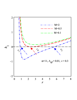
(b)  The locations of the horizons in the metric potential $g_{rr}$

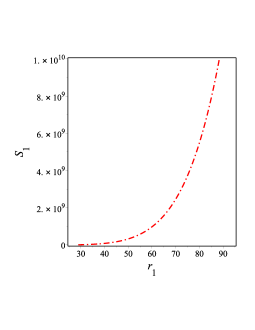
(c)  The characteristics of the entropy

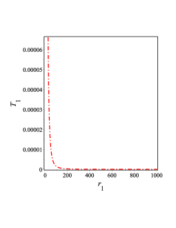
(d)  The temperature according to Hawking

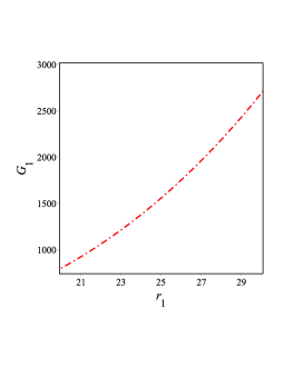
(e)  The characteristics of the Gibbs function

Figure 1: 0(a) The overall trends of the metric potential $g_{rr}$ are illustrated in Fig. 1 for both $v=0$ and $v\neq 0$; 0(b) presents the general tendencies of $g_{rr}$ as $r\to\infty$, revealing three distinct regions; 0(c) showcases the behavior of the entropy; 0(d) depicts the variations in the Hawking temperature; and 0(e) illustrates the pattern of the Gibbs function. All the parameters characterized the model take the values $\Lambda_{eff}=0.1$, $M=v=1$ and $\alpha=-0.1$.

Utilizing Eq. (28), we can determine the entropy associated with the described black hole solution of Eq. (IV) as follows:

$${S_{1}}=\frac{2\pi\left(v\,{r_{1}}^{2}+\sqrt{\left|\alpha\right|}\right)}{3v}.$$ (33)

Examining Eq. (33), it is evident that the charge $v$ is not permitted to assume a zero value. When $\alpha=0$, we cannot recover the typical entropy of GR, primarily because of the constraint imposed by Eq. (19). The entropy trends are illustrated in Fig.1 0(c), showcasing a well-behaved pattern of the entropy.

The Hawking temperature linked to the black hole solution of Eq. (IV) is calculated as:

$${T_{1}}=\frac{\left(6\,{r_{1}}^{6}\Lambda_{eff}-4\,{v}^{3}\sqrt{3}\sqrt{\left|\alpha\right|}-9\,{v}^{2}{r_{1}}^{2}+3\,M{r_{1}}^{3}\right)}{2\pi{r_{1}}^{5}\sqrt{\left({r_{1}}^{2}\Lambda_{eff}+{\frac{{v}^{3}\sqrt{3}\sqrt{\alpha}}{3{r_{1}}^{4}}}+{\frac{3{v}^{2}}{2{r_{1}}^{2}}}-{\frac{M}{r_{1}}}\right)^{2}\left(1+{\frac{v\sqrt{3}\sqrt{\alpha}}{{r_{1}}^{2}}}\right)^{2}}}\,.$$ (34)

Here ${T_{1}}$ represent the temperature of Hawking at the event horizon. The temperature is depicted in Fig. 0(d), revealing that it is always positive.

The grand canonical ensemble’s free energy, which is known as Gibbs free energy, is described as Zheng and Yang (2018); Kim and Kim (2012):

$$G(r_{+})=M(r_{1})-T(r_{1})S(r_{1}),$$ (35)

where $T(r_{h})$, $S(r_{h})$, and $E(r_{h})$ represent the temperature, entropy, and quasilocal energy at the event horizon, respectively. By substituting Eqs. (28), (31), (33), and (34) into (35), we obtain:

$$G(r_{+})=\frac{1}{6}\left\{36v{r_{1}}^{14}{\Lambda_{eff}}^{2}+36{r_{1}}^{12}{\Lambda_{eff}}^{2}{v}^{2}\sqrt{3}\sqrt{\alpha}+132{r_{1}}^{8}\Lambda_{eff}{v}^{4}\sqrt{3}\sqrt{\alpha}+72{r}^{6}\Lambda_{eff}{v}^{5}\alpha+108{r_{1}}^{10}\Lambda_{eff}{v}^{3}-36v{r}^{11}\Lambda_{eff}M\right.$$

$$\left.-36{r_{1}}^{9}\Lambda_{eff}M{v}^{2}\sqrt{3}\sqrt{\alpha}+120{v}^{7}\alpha{r_{1}}^{2}+12{v}^{8}\sqrt{3}{\alpha}^{3/2}+117{v}^{6}\sqrt{3}\sqrt{\alpha}{r_{1}}^{4}-66{v}^{4}\sqrt{3}\sqrt{\alpha}M{r_{1}}^{5}-36{v}^{5}\alpha M{r_{1}}^{3}+81{v}^{5}{r_{1}}^{6}\right.$$

$$\left.-54{v}^{3}{r_{1}}^{7}M-12{r_{1}}^{12}\Lambda_{eff}v-12{r_{1}}^{10}\Lambda_{eff}\sqrt{3}\sqrt{\alpha}+8{r_{1}}^{6}{v}^{4}\sqrt{3}\sqrt{\alpha}+24{r_{1}}^{4}{v}^{3}\alpha+18{r_{1}}^{8}{v}^{3}+18{r_{1}}^{6}{v}^{2}\sqrt{3}\sqrt{\alpha}-6{r_{1}}^{9}Mv\right.$$

$$\left.-6{r}^{7}M\sqrt{3}\sqrt{\alpha}\right\}\left\{{r_{1}}^{3}\left(6{r_{1}}^{6}\Lambda_{eff}+2{v}^{3}\sqrt{3}\sqrt{\alpha}+9{v}^{2}{r}^{2}-6M{r}^{3}\right)\left({r_{1}}^{2}+v\sqrt{3}\sqrt{\alpha}\right)v\right\}^{-1}\,.$$ (36)

The trends of the Gibbs energy for the black hole (IV) are depicted in Fig. 10(e) for specific values of the model parameters. Fig. 10(e) illustrates that the Gibbs free energy is consistently positive, indicating greater global stability.

VII Solutions with multiple horizons

The most basic black hole solution is characterized by the Ads/dS-Schwarzschild metric, where the description of the metric coefficient $g_{00}$ is:

$$f=\Lambda r^{2}-\frac{2M}{r}=f_{1}(r)(r-r_{1})(r-r_{2})(r-r_{3})\,.$$ (37)

Here, $f_{1}(r)=\frac{1}{r}$ and $r_{i},i=1,2,3$ represent the horizons. Equation (37) possesses a single real horizon at $r=r_{1}=\sqrt[3]{2M\Lambda}$, while the other two horizons, $r_{2}$ and $r_{3}$, are imaginary. Equation (37) can be derived from Eq. (IV) when $v=0$. When $v\neq 0$, we derive the solution of Eq. (IV) in the case of four-dimensions in the following manner:

$$h=r^{2}\Lambda_{eff}-\frac{M}{r}+\frac{3v^{2}}{2r^{2}}+\frac{\sqrt{3\left|\alpha\right|}v^{3}}{3r^{4}}=h_{2}(r)(r-r_{1})(r-r_{2})(r-r_{3})(r-r_{4})(r-r_{5})(r-r_{6})\,.$$ (38)

We identify the impact of the quadratic form of non-metricity, generating six roots from which at least three can be extracted. Here, $h_{2}(r)=\frac{1}{r^{4}}$. Now we are going to show that, it is possible to produce at least three real roots of Eq. (38) in the following manner:

$$h=r^{2}\Lambda_{eff}-\frac{M}{r}+\frac{3v^{2}}{2r^{2}}+\frac{\sqrt{3\left|\alpha\right|}v^{3}}{3r^{4}}=h_{2}(r)(r-r_{1})(r-r_{2})(r-r_{3})\,.$$ (39)

In this study, $r_{1}$ and $r_{2}$ stand for the cosmological and event horizons, respectively, while $r_{3}$ is the radius horizon obtained from the contribution of the quadratic form of non-metricity. Deriving the explicit forms of the three horizons for Eq. (IV) poses a challenge. Hence, we will numerically and graphically solve Eq. (IV) in cases where $v<0$. We graph Eq. (IV) regarding certain values of mass, charge, and parameter $\alpha$ related to the quadratic form of non-metricity.

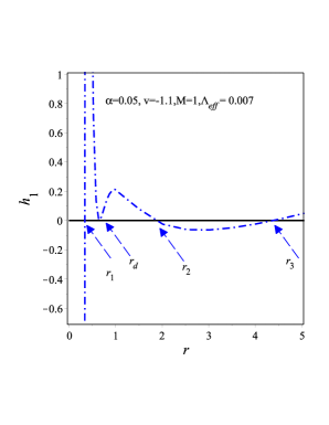
(a)  The BH’s multi-horizon

Figure 2: Multi-horizon plot of Eq. (IV) against coordinate $r$.

In the case of a black hole with one or two horizons, the curvature scalar is recognized to be zero, as observed in the Schwarzschild and Reissner-Nordstr”om solutions. However, for a black hole with more than two horizons, the curvature scalar becomes singular at the center. At $r=0$, the Kretschmann scalar is singular for any black hole with more than one horizon. This is explained in detail by Eq. (V)..

Let’s now examine the thermodynamics of the multi-horizons stated earlier. Because of the negative value of $v$ in the case of multi-horizons, we obtain for BH (IV) that these quantities behave differently thermodynamically. We have stable BHs for a multi-horizon spacetime, as demonstrated by all the charts in Fig. 3. The Hawking temperature in the multi-horizon situation is negative up to $r<r_{d}$ and then positive as $r>r_{d}$, as can be shown in Fig. 3 2(a).

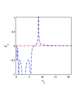
(a)  The Hawking temperature associated with the horizon of the BH described in Eq. (IV)

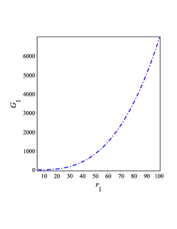
(b)  The the Gibbs function of solution described in Eq. (IV)

Figure 3: Thermodynamic features of the BH solutions (IV) illustrated in diagrams for parameter $v$ taking negative values: 2(a) characteristic pattern of the black hole’s horizon Hawking temperature (IV) and 2(b) the heat capacity of the black hole’s horizon (IV).

VIII Conclusions and discussion

The study of charged cylindrical black holes in the context of the $f(\mathbb{Q})$ gravitational theory has yielded important discoveries about these unusual astronomical objects. The research has included a thorough investigation of how the $f(\mathbb{Q})$ change affects the characteristics and actions of charged cylindrical black holes, providing insight into how gravity and the modified theory interact.

The significant effect of the $f(\mathbb{Q})$ alteration on the geometric and thermodynamic properties of charged cylindrical black holes is one of the main conclusions of this work. The examination of thermodynamic parameters like temperature, heat capacity, and entropy has uncovered fascinating trends that have defied traditional wisdom and opened the door to a more comprehensive comprehension of the underlying gravitational dynamics.

We give here a novel charged solution in the framework of the Maxwell-$f(\mathbb{Q})$ gravitational theory for dimensions $N\geq 4$, with the coincident gauge condition imposed Heisenberg (2023). For $f(\mathbb{Q})=\mathbb{Q}+\frac{1}{2}\alpha\mathbb{Q}^{2}$, where $\alpha<0$, we find a particular solution. Interesting aspects are shown by this solution, which includes both quadrupole and monopole terms. The requirement that the metric asymptotically approaches Anti-de Sitter (AdS) governs how these terms interact.

Additionally, we explored the singularity innate to this solution and clarified that there is a singularity at $r=0$ for any invariant derived from the curvature and non-metricity. In comparison with the singularity of a charged black hole in GR, this singularity is less severe. The invariants asymptotic behavior is given as $K=\mathbb{R}{\mu\nu}\mathbb{R}^{\mu\nu}=\mathbb{R}=\mathbb{Q}^{\alpha\beta\gamma}\mathbb{Q}{\alpha\beta\gamma}=\mathbb{Q}^{\alpha}\mathbb{Q}{\alpha}=\tilde{\mathbb{Q}}^{\alpha}\tilde{\mathbb{Q}}{\alpha}=\mathbb{Q}\sim r^{-(N-2)}$, in opposition to the behavior seen in established solutions within GR’s Einstein-Maxwell theory. Furthermore, the non-charged solution obtained in this work, according to Eq. (III), shows characteristics in such a way that $K=\mathbb{R}{\mu\nu}\mathbb{R}^{\mu\nu}\sim r^{-2N}$ and $\mathbb{R}\sim r^{-N}$. Moreover, despite the fact that the charged solution possesses distinct constituents of $g{tt}$ and $g^{rr}$, the event horizons and Killing horizons of both cases coincide.

From a genuine physical perspective, these entities can contribute to the current discussion on whether gravity model is the most reliable, be it curvature or non-metricity picture. As explained in literature, since GR is substantially equivalent, the discussion should center on $f(\mathbb{Q})$ and $f(\mathbb{R})$ constructions because they are essentially different. Even basic concepts such as gravitational waves show significant differences between $f(\mathbb{Q})$ and $f(\mathbb{R})$ formulations, as Soudi et al. (2019) illustrates. In resolving this dispute, a thorough grasp of black hole properties may be extremely helpful.

References

- Heisenberg (2023) L. Heisenberg (2023), eprint 2309.15958.
- Maurya et al. (2023) S. K. Maurya, K. N. Singh, M. Govender, G. Mustafa, and S. Ray, Astrophys. J. Suppl. 269, 35 (2023), eprint 2309.10130.
- Unzicker and Case (2005) A. Unzicker and T. Case (2005), eprint physics/0503046.
- Nester and Yo (1999) J. M. Nester and H.-J. Yo, Chin. J. Phys. 37, 113 (1999), eprint gr-qc/9809049.
- Ferraro and Fiorini (2007) R. Ferraro and F. Fiorini, Phys. Rev. D 75, 084031 (2007), eprint gr-qc/0610067.
- Beltrán Jiménez et al. (2018a) J. Beltrán Jiménez, L. Heisenberg, and T. Koivisto, Phys. Rev. D 98, 044048 (2018a), eprint 1710.03116.
- Bengochea and Ferraro (2009) G. R. Bengochea and R. Ferraro, Phys. Rev. D 79, 124019 (2009), eprint 0812.1205.
- Linder (2010) E. V. Linder, Phys. Rev. D 81, 127301 (2010), [Erratum: Phys.Rev.D 82, 109902 (2010)], eprint 1005.3039.
- Bamba et al. (2011) K. Bamba, C.-Q. Geng, C.-C. Lee, and L.-W. Luo, JCAP 01, 021 (2011), eprint 1011.0508.
- Bamba et al. (2010) K. Bamba, C.-Q. Geng, and C.-C. Lee (2010), eprint 1008.4036.
- Narawade et al. (2022) S. A. Narawade, L. Pati, B. Mishra, and S. K. Tripathy, Phys. Dark Univ. 36, 101020 (2022), eprint 2203.14121.
- Solanki et al. (2022a) R. Solanki, A. De, S. Mandal, and P. K. Sahoo, Phys. Dark Univ. 36, 101053 (2022a), eprint 2201.06521.
- Solanki et al. (2022b) R. Solanki, A. De, and P. K. Sahoo, Phys. Dark Univ. 36, 100996 (2022b), eprint 2203.03370.
- Atayde and Frusciante (2021) L. Atayde and N. Frusciante, Phys. Rev. D 104, 064052 (2021), eprint 2108.10832.
- Beltrán Jiménez et al. (2019) J. Beltrán Jiménez, L. Heisenberg, and T. S. Koivisto, Universe 5, 173 (2019), eprint 1903.06830.
- D’Ambrosio et al. (2022) F. D’Ambrosio, L. Heisenberg, and S. Kuhn, Class. Quant. Grav. 39, 025013 (2022), eprint 2109.04209.
- Lu et al. (2021) J. Lu, Y. Guo, and G. Chee (2021), eprint 2108.06865.
- Capozziello et al. (2022) S. Capozziello, V. De Falco, and C. Ferrara, Eur. Phys. J. C 82, 865 (2022), eprint 2208.03011.
- Aldrovandi and Pereira (2013) R. Aldrovandi and J. G. Pereira, Teleparallel Gravity: An Introduction (Springer, 2013), ISBN 978-94-007-5142-2, 978-94-007-5143-9.
- Maluf (2013) J. W. Maluf, Annalen Phys. 525, 339 (2013), eprint 1303.3897.
- Dialektopoulos et al. (2019) K. F. Dialektopoulos, T. S. Koivisto, and S. Capozziello, Eur. Phys. J. C 79, 606 (2019), eprint 1905.09019.
- Barros et al. (2020) B. J. Barros, T. Barreiro, T. Koivisto, and N. J. Nunes, Phys. Dark Univ. 30, 100616 (2020), eprint 2004.07867.
- Beltrán Jiménez et al. (2020) J. Beltrán Jiménez, L. Heisenberg, T. S. Koivisto, and S. Pekar, Phys. Rev. D 101, 103507 (2020), eprint 1906.10027.
- Bajardi et al. (2020) F. Bajardi, D. Vernieri, and S. Capozziello, Eur. Phys. J. Plus 135, 912 (2020), eprint 2011.01248.
- Ayuso et al. (2021) I. Ayuso, R. Lazkoz, and V. Salzano, Phys. Rev. D 103, 063505 (2021), eprint 2012.00046.
- Flathmann and Hohmann (2021) K. Flathmann and M. Hohmann, Phys. Rev. D 103, 044030 (2021), eprint 2012.12875.
- Khyllep et al. (2021) W. Khyllep, A. Paliathanasis, and J. Dutta, Phys. Rev. D 103, 103521 (2021), eprint 2103.08372.
- D’Ambrosio et al. (2020) F. D’Ambrosio, M. Garg, and L. Heisenberg, Phys. Lett. B 811, 135970 (2020), eprint 2004.00888.
- Adak and Sert (2005) M. Adak and O. Sert, Turk. J. Phys. 29, 1 (2005), eprint gr-qc/0412007.
- Adak et al. (2006) M. Adak, M. Kalay, and O. Sert, Int. J. Mod. Phys. D 15, 619 (2006), eprint gr-qc/0505025.
- Adak et al. (2013) M. Adak, O. Sert, M. Kalay, and M. Sari, Int. J. Mod. Phys. A 28, 1350167 (2013), eprint 0810.2388.
- Mol (2017) I. Mol, Adv. Appl. Clifford Algebras 27, 2607 (2017), eprint 1406.0737.
- Beltrán Jiménez et al. (2018b) J. Beltrán Jiménez, L. Heisenberg, and T. S. Koivisto, JCAP 08, 039 (2018b), eprint 1803.10185.
- Gakis et al. (2020) V. Gakis, M. Krššák, J. Levi Said, and E. N. Saridakis, Phys. Rev. D 101, 064024 (2020), eprint 1908.05741.
- Järv et al. (2018) L. Järv, M. Rünkla, M. Saal, and O. Vilson, Phys. Rev. D 97, 124025 (2018), eprint 1802.00492.
- Heisenberg (2019) L. Heisenberg, Phys. Rept. 796, 1 (2019), eprint 1807.01725.
- De Felice and Tsujikawa (2010) A. De Felice and S. Tsujikawa, Living Reviews in Relativity 13, 1 (2010).
- Sotiriou and Faraoni (2010) T. P. Sotiriou and V. Faraoni, Reviews of Modern Physics 82, 451 (2010).
- Cai et al. (2016) Y.-F. Cai, S. Capozziello, M. De Laurentis, and E. N. Saridakis, Rept. Prog. Phys. 79, 106901 (2016), eprint 1511.07586.
- Bahamonde et al. (2023) S. Bahamonde, K. F. Dialektopoulos, C. Escamilla-Rivera, G. Farrugia, V. Gakis, M. Hendry, M. Hohmann, J. Levi Said, J. Mifsud, and E. Di Valentino, Rept. Prog. Phys. 86, 026901 (2023), eprint 2106.13793.
- Bamba et al. (2012) K. Bamba, S. Capozziello, S. Nojiri, and S. D. Odintsov, Astrophys. Space Sci. 342, 155 (2012), eprint 1205.3421.
- Bamba et al. (2013) K. Bamba, S. D. Odintsov, and D. Sáez-Gómez, Phys. Rev. D 88, 084042 (2013), eprint 1308.5789.
- Casalino et al. (2021) A. Casalino, B. Sanna, L. Sebastiani, and S. Zerbini, Phys. Rev. D 103, 023514 (2021), eprint 2010.07609.
- Zhao (2022) D. Zhao, Eur. Phys. J. C 82, 303 (2022), eprint 2104.02483.
- Lazkoz et al. (2019) R. Lazkoz, F. S. N. Lobo, M. Ortiz-Baños, and V. Salzano, Phys. Rev. D 100, 104027 (2019), eprint 1907.13219.
- Mandal et al. (2020) S. Mandal, P. K. Sahoo, and J. R. L. Santos, Phys. Rev. D 102, 024057 (2020), eprint 2008.01563.
- Capozziello and Shokri (2022) S. Capozziello and M. Shokri, Phys. Dark Univ. 37, 101113 (2022), eprint 2209.06670.
- Capozziello and D’Agostino (2022) S. Capozziello and R. D’Agostino, Phys. Lett. B 832, 137229 (2022), eprint 2204.01015.
- Hu et al. (2022) K. Hu, T. Katsuragawa, and T. Qiu, Phys. Rev. D 106, 044025 (2022), eprint 2204.12826.
- Nashed (2013a) G. G. L. Nashed, Phys. Rev. D 88, 104034 (2013a), eprint 1311.3131.
- Capozziello et al. (2013) S. Capozziello, P. A. Gonzalez, E. N. Saridakis, and Y. Vasquez, JHEP 02, 039 (2013), eprint 1210.1098.
- Nashed (2013b) G. G. L. Nashed, Gen. Rel. Grav. 45, 1887 (2013b), eprint 1502.05219.
- Mann (1997) R. B. Mann, Annals Israel Phys. Soc. 13, 311 (1997), eprint gr-qc/9709039.
- Lemos (1995) J. P. S. Lemos, Phys. Lett. B 353, 46 (1995), eprint gr-qc/9404041.
- Awad and Johnson (2000a) A. M. Awad and C. V. Johnson, Phys. Rev. D 61, 084025 (2000a), eprint hep-th/9910040.
- Awad and Johnson (2000b) A. M. Awad and C. V. Johnson, Phys. Rev. D 62, 125010 (2000b), eprint hep-th/0006037.
- Aharony et al. (2000) O. Aharony, S. S. Gubser, J. M. Maldacena, H. Ooguri, and Y. Oz, Phys. Rept. 323, 183 (2000), eprint hep-th/9905111.
- Banerjee et al. (2021) A. Banerjee, A. Pradhan, T. Tangphati, and F. Rahaman, Eur. Phys. J. C 81, 1031 (2021), eprint 2109.15105.
- Lin and Zhai (2021) R.-H. Lin and X.-H. Zhai, Phys. Rev. D 103, 124001 (2021), [Erratum: Phys.Rev.D 106, 069902 (2022)], eprint 2105.01484.
- Awad et al. (2017) A. M. Awad, S. Capozziello, and G. G. L. Nashed, JHEP 07, 136 (2017), eprint 1706.01773.
- Tipler (1977) F. J. Tipler, Phys. Lett. A 64, 8 (1977).
- Clarke and Królak (1985) C. Clarke and A. Królak, Journal of Geometry and Physics 2, 127 (1985).
- Nashed and Nojiri (2023) G. G. L. Nashed and S. Nojiri, Phys. Rev. D 107, 064069 (2023), eprint 2303.07349.
- Mazharimousavi (2023) S. H. Mazharimousavi, Eur. Phys. J. C 83, 406 (2023), [Erratum: Eur.Phys.J.C 83, 597 (2023)], eprint 2304.12935.
- Sheykhi (2012) A. Sheykhi, Phys. Rev. D 86, 024013 (2012), eprint 1209.2960.
- Sheykhi (2010) A. Sheykhi, Eur. Phys. J. C 69, 265 (2010), eprint 1012.0383.
- Hendi et al. (2010) S. H. Hendi, A. Sheykhi, and M. H. Dehghani, Eur. Phys. J. C 70, 703 (2010), eprint 1002.0202.
- Sheykhi et al. (2010) A. Sheykhi, M. H. Dehghani, and S. H. Hendi, Phys. Rev. D 81, 084040 (2010), eprint 0912.4199.
- Cognola et al. (2011) G. Cognola, O. Gorbunova, L. Sebastiani, and S. Zerbini, Phys. Rev. D 84, 023515 (2011), eprint 1104.2814.
- Zheng and Yang (2018) Y. Zheng and R.-J. Yang, Eur. Phys. J. C 78, 682 (2018), eprint 1806.09858.
- Nouicer (2007) K. Nouicer, Class. Quant. Grav. 24, 5917 (2007), [Erratum: Class.Quant.Grav. 24, 6435 (2007)], eprint 0706.2749.
- Chamblin et al. (1999) A. Chamblin, R. Emparan, C. V. Johnson, and R. C. Myers, Phys. Rev. D 60, 064018 (1999), eprint hep-th/9902170.
- Kim and Kim (2012) W. Kim and Y. Kim, Phys. Lett. B 718, 687 (2012), eprint 1207.5318.
- Soudi et al. (2019) I. Soudi, G. Farrugia, V. Gakis, J. Levi Said, and E. N. Saridakis, Phys. Rev. D 100, 044008 (2019), eprint 1810.08220.