PUMA: Efficient Continual Graph Learning with Graph Condensation

Abstract

When handling streaming graphs, existing graph representation learning models encounter a catastrophic forgetting problem, where previously learned knowledge of these models is easily overwritten when learning with newly incoming graphs. In response, Continual Graph Learning (CGL) emerges as a novel paradigm enabling graph representation learning from static to streaming graphs. Our prior work, Condense and Train (CaT) [1] is a replay-based CGL framework with a balanced continual learning procedure, which designs a small yet effective memory bank for replaying data by condensing incoming graphs. Although the CaT alleviates the catastrophic forgetting problem, there exist three issues: (1) The graph condensation algorithm derived in CaT only focuses on labelled nodes while neglecting abundant information carried by unlabelled nodes; (2) The continual training scheme of the CaT overemphasises on the previously learned knowledge, limiting the model capacity to learn from newly added memories; (3) Both the condensation process and replaying process of the CaT are time-consuming. In this paper, we propose a PsUdo-label guided Memory bAnk (PUMA) CGL framework, extending from the CaT to enhance its efficiency and effectiveness by overcoming the above-mentioned weaknesses and limits. To fully exploit the information in a graph, PUMA expands the coverage of nodes during graph condensation with both labelled and unlabelled nodes. Furthermore, a training-from-scratch strategy is proposed to upgrade the previous continual learning scheme for a balanced training between the historical and the new graphs. Besides, PUMA uses a one-time prorogation and wide graph encoders to accelerate the graph condensation and the graph encoding process in the training stage to improve the efficiency of the whole framework. Extensive experiments on four datasets demonstrate the state-of-the-art performance and efficiency over existing methods. The code has been released in https://github.com/superallen13/PUMA.

1 Introduction

Graph representation learning aims to model the graph-structured data, typically in recommender systems [2], traffic prediction [3] and protein function prediction [4]. Generally, graphs are treated as static data in traditional graph representation learning, where a model is fixed once it has been trained. However, for many scenarios in the real world (e.g., social networks, cation networks and knowledge graphs), graph data are changing and evolving in a streaming manner [5, 6, 7]. Recently, the Continual graph learning (CGL) has emerged to handle the streaming graph by adapting the static graph neural networks (GNNs). In CGL, the most significant challenge is how to address a catastrophic forgetting problem, where a model easily forgets the previously learned knowledge while overemphasising on the incoming graphs [8, 9, 10, 1].

A few attempts have been made to tackle this catastrophic forgetting problem through leveraging regularisation penalty [9], architecture redesign [11], and replayed graphs [8, 10]. Among all, the replay-based methods achieve the best model performance and flexibility by storing and replaying a memory bank, which contains either informative nodes [8] or subgraphs [10]. In our previous work, the Condensed and Train (CaT) [1] was proposed to enhance the efficacy of memory banks and the balanced learning. The CaT consists of two main modules: a Condensed Graph Memory (CGM), which continually condenses incoming graphs to small yet informative replayed graphs, and a Train in Memory (TiM), which trains the CGL model only using the memory bank where replayed graphs have similar sizes to guarantee the balanced learning.

Although our previous CaT framework [1] has demonstrated that the incoming graphs can be successfully condensed to an extremely small scale, for example, 0.1% of the original size, for the continual learning, it remains a few challenges in further improving the efficacy and efficiency. (1) Neglected unlabelled nodes: In the previous condensation process, nodes without label will be considered as the target for condensation rather than just supporting the message passing for the labelled nodes, potentially overlooking the valuable information from unlabelled nodes. (2) Imbalanced learned knowledge: Since previously generated memories will be repeatedly replayed during the continual learning, historical knowledge is easier to retain while the perception of new information in incoming graphs is hindered. Figure 1 shows this situation for CGL that the CaT model converges faster and better for the knowledge from previous Task 0 with a smaller loss than the newly incoming Task 1. This is due to the fact that neural networks are prone to learn shortcuts from training data [12]. (3) Low efficiency: Both the condensation and the CGL training are inefficient, because of repetitive computations, slow convergence speed of condensation and unnecessary message passing in the GNN training. The condensation process requires to repeatedly map the incoming graphs to different embedding spaces, which causes a large number of recalculations for message passing among node neighbourhoods. Besides, condensed graph converging is impeded by narrow graph encoders (e.g., encoders with 512-dimensional hidden layers). Furthermore, message aggregations of neighbours on the edge-free replayed memories is redundant, which hinders the efficiency of CGL model training.

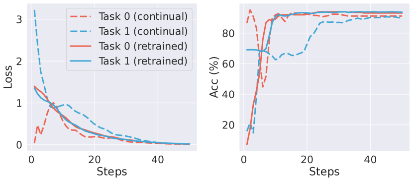
Figure 1: Loss and accuracy comparisons for the first two tasks when training replayed graph of Task 1 while replaying the replayed graph of Task 0 at the first 50 steps after the replayed graph of Task 0 has been learned 500 steps. The continual (dotted lines) and retrained (solid lines) loss values for Task 0 (red) and Task 1 (blue) are shown, providing a visual representation of an optimisation problem.

In light of the above challenges in the CaT method for CGL, this paper proposes a novel PseUdo-label guided Memory bAnk (PUMA) CGL framework to extend the CaT in a more effective and efficient manner. Firstly, the PUMA framework develops a pseudo-labelling to integrate data from unlabelled nodes, enhancing the informativeness of the memory bank, which addresses the issue of neglected unlabelled nodes. Secondly, to tackle the inflexible historical knowledge problem, a retraining strategy is devised. This involves initialising the entire model before replaying to balance the learned knowledge among different tasks for more effective decision boundaries as well as ensuring a more stable learning process. Figure 1 represents the optimisation process is smother, and the converge speed is quicker after using retraining scheme. Lastly, the repetitive message passing calculation in the condensation process is simplified via a one-time propagation method, which aggregates messages from neighbouring nodes across the entire incoming graph one time, and it can be stored for reuse, significantly reducing the computational effort. Furthermore, wide graph encoders including more neurons are developed to accelerate convergence during condensation, enhancing the update efficiency of the condensed memories. Finally, to improve the training efficiency of the CGL model, the training of a multilayer perceptron (MLP) in lieu of message-passing GNNs is proposed. Due to its edge-free nature, PUMA enables the MLP to learn feature extractions and utilises a GNN to inference on the graphs with edges. These solutions collectively enhance the efficacy and efficiency of the graph condensation-based CGL framework.

To sum up, this paper proposes a novel PUMA CGL framework extended from our previous CaT [1] method with following substantial new contributions:

• A Pseudo-label guided memory bank is proposed to condense not only labelled nodes but unlabelled nodes leveraging the information from the full graph.

• A retraining strategy is devised in the replay phase to alleviate the imbalanced learned knowledge problem, resulting in a promising overall performance.

• The condensation and the training speed is significantly improved without compromising the performance in light of the innovations consisting of a newly developed one-time propagation, wide graph encoders and MLP training with edge-free memories.

• Extensive experiments and in-depth analysis are conducted on four datasets, showcasing the effectiveness and the efficiency of the PUMA.

2 Related Work

2.1 Graph Neural Networks

Graph Neural Networks (GNNs) are effective tools for graph-based tasks [13, 14, 15, 16]. GCN [17] employs Laplacian normalisation for message propagation. GAT [18] is proposed to use the attention mechanism [19] for message passing. SGC [20] simplifies GCN by removing the non-linear activation operation. GraphSAGE [21] uses node sampling to deal with large-scale graph representation learning.

2.2 Continual Graph Learning

Continual graph learning is a task for handling streaming graph data. Continual learning has been studied in computer vision [22, 23, 24, 25]. In graph area, CGL methods can be categorised into three branches: regularisation [9], replay- [8, 10], and architecture-based [11] methods. TWP [9] preserves the topological information of historical graphs by adding regularisation. HPNs [11] redesigns the GNN architecture to 3-layer prototypes for representation learning. ER-GNN [8] integrates memory-replay by storing representative nodes. Sparsified subgraph memory (SSM) [10] stores the sparisified subgraphs by dropping edges and nodes randomly or basing on the node degree. Differing from SSM, which sparsifies the incoming graph based on the degree or randomly selected central nodes’ neighbours, SEM-curvature [26] employs balanced Forman curvature to compute edges containing the most informative content to maximise structural information within the subgraph. Considering the inter connections between tasks, the structure shift also leads to catastrophic forgetting problem. Structural shift risk mitigation (SSRM) [27] uses regularisation-based techniques to mitigate this issue. Two recent benchmarks [28, 29] have been developed for CGL.

2.3 Graph Condensation

Dataset condensation generates a small and synthetic dataset to replace the original dataset and to train a model with similar performance. Dataset condensation has been applied in computer vision [30, 31, 32, 33, 34, 35]. Recently, gradient matching has been applied to graph condensation, such as GCond [36], DosCond [37] and MCond [38]. DM [34] aims to learn synthetic samples which have similar distribution with the original dataset to mimic sampling methods [39, 40, 41]. GCDM [42] uses the distribution matching for graph condensation. SFGC [43] uses a training trajectory meta-matching scheme to condensed the original graph into edge-free graphs. SGDD [44] broadcasts the structure information of original graph to condensed graph in the spectral graph theory perspective.

Recent attempts on computer vision have directly applied dataset condensation to continual learning [45, 46, 47, 48, 49]. Our previous work CaT [1] applies graph condensation to graph continual learning while ensuring the balanced training.

3 Preliminary

In the following, a bold lowercase letter denotes a vector, a bold uppercase letter denotes a matrix, a general letter denotes a scalar, and a scripted uppercase letter denotes a set.

3.1 Graph

For a node classification problem, a graph is denoted as $\mathcal{G}=\{\boldsymbol{A},\boldsymbol{X},\boldsymbol{Y}\}$, where $\boldsymbol{X}\in\mathbb{R}^{n\times d}$ is the $d$-dimensional feature matrix for $n$ nodes, and the adjacency matrix $\boldsymbol{A}\in\mathbb{R}^{n\times n}$ denotes the graph structure. In this paper, the graph is undirected and unweighted. $\boldsymbol{Y}\in\mathbb{R}^{n\times 1}$ includes node labels from a class set $\mathcal{C}$.

3.2 Graph Neural Networks

Graph Neural Networks (GNNs) are tools for representation learning in node classification problems. The node representation in GNN is calculated by aggregating messages from neighbouring nodes. GNN can be represented as a function:

$$\boldsymbol{E}=\text{GNN}_{\theta}(\boldsymbol{A},\boldsymbol{X}),$$ (1)

where $\theta$ is the model parameter and $\boldsymbol{E}\in\mathbb{R}^{n\times d^{\prime}}$ denotes $d^{\prime}$-dimensional node embeddings. For example, the following is the output $\boldsymbol{E}^{(0)}$ of the fist layer of a typical Graph Convolutional Network (GCN):

$$\boldsymbol{E}^{(0)}=\sigma(\boldsymbol{L}\boldsymbol{X}\boldsymbol{W}^{(0)}),$$ (2)

where $\boldsymbol{L}=\boldsymbol{D}^{-\frac{1}{2}}\boldsymbol{A}\boldsymbol{D}^{-\frac{1}{2}}$ is the normalised Laplacian adjacent matrix, and $\boldsymbol{D}$ is the degree matrix. $\boldsymbol{W}^{(0)}\in\mathbb{R}^{d\times d^{\prime}}$ is weights of the first convolutional layer. $\sigma(\cdot)$ is the activation operation for improving the model’s non-linearity.

3.3 Graph Condensation

Graph condensation aims to synthesis a small graph $\mathcal{\tilde{G}}=\{\boldsymbol{\tilde{A}},\boldsymbol{\tilde{X}},\boldsymbol{\tilde{Y}}\}$ for a large graph $\mathcal{G}=\{\boldsymbol{A},\boldsymbol{X},\boldsymbol{Y}\}$. The model trained with the synthetic graph is expected to have a similar performance as with the original graph. This objective is:

$$\min_{\tilde{\mathcal{G}}}\mathcal{L}(\mathcal{G};\tilde{\theta}),\quad\text{s.t.\ }\tilde{\theta}=\operatorname*{arg\,min}_{\theta}\mathcal{L}(\tilde{\mathcal{G}};\theta),$$ (3)

where $\mathcal{L}$ is a task-related loss function, e.g., cross-entropy for classification problems, and $\theta$ is the parameter of GNN.

3.4 Node Classification in Continual Graph Learning

For solving the original node classification problem, GNN uses a full-connected layer to infer the nodes label. For example, after getting the embedding $\boldsymbol{E}^{(0)}$ in Eq. 2, the predicted labels can be inferred by

$$\boldsymbol{\hat{Y}}=\text{Softmax}(\boldsymbol{L}\boldsymbol{X}\boldsymbol{E}^{(0)}\boldsymbol{W}^{(1)}).$$ (4)

In node classification of CGL, a model is required to handle $K$ tasks $\{\mathcal{T}_{1},\mathcal{T}_{2},...\mathcal{T}_{K}\}$. For the $k_{th}$ task $\mathcal{T}_{k}$, an incoming graph $\mathcal{G}_{k}$ arrives and the model needs to be updated with $\mathcal{G}_{k}$ while be tested on all previous graphs and the incoming graph. Following [9, 8, 10], the setting is transductive learning and can be easily extended to inductive learning.

CGL problem has two different continual settings, task incremental learning (task-IL) and class incremental learning (class-IL). In task-IL, the model is only required to distinguish nodes in the same task. While in class-IL, the model is required to classify nodes from all tasks together. Class-IL is more challenging, and this paper focuses on this setting while also reporting the overall performance under task-IL.

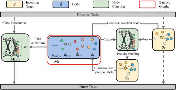
Figure 2: Details of edge-free graph condensation with pseudo-labelling and retraining. PUMA condenses the incoming graph $\mathcal{G}_{k}$ to $\mathcal{\tilde{G}}_{k}$ first, an extra classifier is trained by the memory bank $\mathcal{M}_{k}$ to assign pseudo labels to $\mathcal{G}_{k}$. After that, $\mathcal{G}_{k}$ is condensed again to update the $\mathcal{M}_{k}$. The MLP model is initialised first and trained by the $\mathcal{G}_{k}$.

4 Methodology

This section describes the details of the proposed PseUdo-label guided Memory bAnk (PUMA) framework. The framework details are shown in Fig. 2. PUMA first condenses the incoming graph considering unlabelled nodes with pseudo labels. Once PUMA is updated, model initialises all weights and trains with PUMA from scratch.

4.1 Fast Graph Condensation by Distribution Matching

Condensation-based memory bank stores condensed synthetic graphs to approximate the historical data distribution. In this section, we develop a efficient graph condensation with distribution matching, aiming to maintain a similar data distribution for the synthetic data as the original data. This approach serves as a replayed graph generation method.

For Task $\mathcal{T}_{k}$, the incoming graph $\mathcal{G}_{k}=\{\boldsymbol{A}_{k},\boldsymbol{X}_{k},\boldsymbol{Y}_{k}\}$, a edge-free condensed graph $\mathcal{\tilde{G}}_{k}=\{\boldsymbol{\tilde{X}}_{k},\boldsymbol{\tilde{Y}}_{k}\}$ is generated by graph condensation. Compared with Eq. 3, under the distribution matching scheme, the objective function of graph condensation here can be reformulated as follows:

$$\mathcal{\tilde{G}}_{k}^{*}=\operatorname*{arg\,min}_{\mathcal{\tilde{G}}_{k}}\text{Dist}(\mathcal{G}_{k},\mathcal{\tilde{G}}_{k}),$$ (5)

where $\text{Dist}(\cdot,\cdot)$ function calculates the distance between two graphs. Using distribution matching, the distance between two graphs is measured in the embedding space, where both graphs are encoded by the same encoder. CaT encodes the original graph with a specific dimensional GNN encoder and randomly initialises the encoder weights for better generalisation performance. PUMA disentangles feature propagation and feature transformation the graph encoding. The incoming graph only propagates once to avoid calculate the feature aggregation of the incoming graph repeatedly but retain the structural information of the incoming graph naturally. Aggregated features $\boldsymbol{F}$ of the original graph can be calculated as a pre-processing:

$$\boldsymbol{F}=\boldsymbol{L}\boldsymbol{X},$$ (6)

where $\boldsymbol{L}$ is the normalised Laplacian adjacent matrix, and $\boldsymbol{X}$ is the nodes features of the original graph. Feature transformation can use a wide multilayer perceptron with randomly initialised weights $\theta$ ($\text{MLP}_{\theta}$):

$$\mathcal{\tilde{G}}_{k}^{*} =\operatorname*{arg\,min}_{\mathcal{\tilde{G}}_{k}}\text{Dist}(\text{MLP}_{\theta}(\boldsymbol{\tilde{F}}),\text{MLP}_{\theta}(\boldsymbol{\tilde{X}}_{k}))$$ (7)

$$=\operatorname*{arg\,min}_{\mathcal{\tilde{G}}_{k}}\text{Dist}(\boldsymbol{E}_{k},\boldsymbol{\tilde{E}}_{k}),$$ (8)

where ${\mathcal{\tilde{G}}}_{k}^{*}=\{\boldsymbol{\tilde{X}}_{k}^{*},\boldsymbol{\tilde{Y}}_{k}^{*}\}$ is the optimal replayed graph with distribution close to the distribution of the incoming graph. Maximum mean discrepancy (MMD) is used to empirically calculate the distribution distance between two graphs. The objective is to find an optimal $\mathcal{\tilde{G}}_{k}$ for MMD:

$$\ell_{\text{MMD}}=\sum_{c\in\mathcal{C}_{k}}r_{c}\cdot||\text{Mean}(\boldsymbol{E}_{k,c})-\text{Mean}(\boldsymbol{\tilde{E}}_{k,c})||^{2},$$ (9)

where $\mathcal{C}_{k}$ is the set of classes of nodes in $\mathcal{G}_{k}$, $\boldsymbol{E}_{c,k}$ and $\boldsymbol{\tilde{E}}_{c,k}$ are the embedding matrix of the incoming graph and condensed graph, respectively, where all nodes’ labels are $c_{k}$, and $r_{c,k}=\frac{|\boldsymbol{E}_{c,k}|}{|\boldsymbol{E}_{k}|}$ is the class ratio for class $c_{k}$. $|\cdot|$ is the number of rows in a matrix. $\text{Mean}(\cdot)$ is the mean vector of the node embeddings.

To efficiently operate the condensation procedure, the feature encoders with random weights are employed here without training. The objective of the distribution matching is to minimise the embedding distance in different embedding spaces given by GNNs with random parameters $\theta_{p}$:

$$\min_{\mathcal{\tilde{G}}_{k}}\sum_{\theta_{p}\sim\Theta}\ell_{\text{MMD},\theta_{p}},$$ (10)

where $\Theta$ indicates the whole parameter space.

With the limit of a budget as $b$, node labels $\boldsymbol{\tilde{Y}}\in\mathcal{C}_{k}^{b}$ for the condensed graph is initialised and kept as the same class ratio as the original graph (i.e., for any class $c_{k}$, $r_{k,c}\approx\tilde{r}_{k,c}$). Random sampling from the incoming graph is used to initialise the condensed node features $\boldsymbol{\tilde{X}}_{k}\in\mathbb{R}^{b\times d}$ at the beginning based on the assigned label. The initialisation can also be implemented as random noise.

4.2 Pseudo Label-guided Edge-free Memory Bank

Pseudo-labelling technique is wildly used on the semi-supervised classification problem. It can enlarge the training dataset [50] and provide additional supervision signal [51]. Distribution matching involves calculating class centres of training set for the original and condensed dataset in the embedding space and aligning these centres of the condensed dataset with the counterpart of original one. The more original data points involved in the calculation, the more accurate the centre is. Therefore, unlabelled nodes with pseudo labels can be used to enlarge the training set during graph condensation.

The unlabelled node in the incoming graph will be assigned pseudo labels by a classifier trained by the existing memory bank and the condensed memory of newly incoming graph without pseudo labels. On the other hand, adding more incorrect pseudo labels may negatively affect the distribution matching performance. Therefore, only the pseudo labels that have high confidence scores are added to the distribution matching. Logits of a node $v$ from a classifier are inputted into the Softmax function to get the confidence distribution of different classes:

$$\text{confidence}(v)=\text{max}(\text{Softmax}(\textbf{A},\textbf{X})_{[v,:]})).$$ (11)

After obtaining confidence scores of pseudo labels, a threshold can be used to filter out the more certain pseudo labels for reducing the noisy labels. Distribution matching algorithm can enjoy the enlarged training set to accurately condense. The overall procedure of PUMA is shown in Algorithm 1.

Input: Incoming graph $\mathcal{G}_{k}=\{\boldsymbol{A}_{k},\boldsymbol{X}_{k},\boldsymbol{Y}_{k}\}$, budget $b_{k}$ for the replayed graph $\mathcal{\tilde{G}}_{k}$, memory bank $\mathcal{M}_{k-1}$

Output: $\mathcal{\tilde{G}}_{k}=\{\boldsymbol{\tilde{X}}_{k},\boldsymbol{\tilde{Y}}_{k}\}$

1 Initialise labels of condensed graph $\boldsymbol{\tilde{Y}}_{k}$ by sampling from the label distribution of $\mathcal{G}_{k}$;

2 Initialise node features of condensed graph $\boldsymbol{\tilde{X}}_{k}$ by randomly sampling $b_{k}$ node features from $\boldsymbol{X}_{k}$;

3 Initialise a MLP encoder $\text{MLP}_{\theta}$ and a GNN encoder $\text{GNN}_{\theta}$ with shared parameters $\theta$;

4 for $m\leftarrow 1$ to $M$ do

5       Initialise parameters of MLP and GNN encoders to $\theta_{m}$;

6       for $c_{k}\leftarrow 0$ to $|\mathcal{C}_{k}|-1$ do

7             $E_{c,k}=\text{GNN}_{\theta_{m}}(\boldsymbol{A}_{k},\boldsymbol{X}_{k})$

8             $\tilde{E}_{c,k}=\text{MLP}_{\theta_{m}}(\boldsymbol{\tilde{X}}_{k})$

9             Calculate $\ell_{\text{MMD},\theta_{m}}$ according to Eq. 9

             $\boldsymbol{\tilde{X}}_{k}\leftarrow\boldsymbol{\tilde{X}}_{k}-\eta\nabla_{\boldsymbol{\tilde{X}}_{k}}\ell_{\text{MMD},\theta_{m}}$ ;

              /* $\eta$ is learning rate */

10            

11       end for

12      

13 end for

14

15Train a classifier $\text{GNN}_{PL}$ using $\mathcal{M}_{k-1}$ and $\mathcal{\tilde{G}}_{k}$ to generate pseudo labels $\boldsymbol{Y}_{k,PL}$ for tested/unlabelled nodes in the $\mathcal{G}_{k}$;

16

17for $n\leftarrow 1$ to $N$ do

18       Initialise parameter of MLP and GNN to $\theta_{n}$;

19       for $c_{k}\leftarrow 0$ to $|\mathcal{C}_{k}|-1$ do

20             $E_{c,k}=\text{GNN}_{\theta_{n}}(\boldsymbol{A}_{k},\boldsymbol{X}_{k})$

21             $\tilde{E}_{c,k}=\text{MLP}_{\theta_{n}}(\boldsymbol{\tilde{X}}_{k})$

22             Calculate $\ell_{\text{MMD},\theta_{n}}$ according to Eq. 9

             $\boldsymbol{\tilde{X}}_{k}\leftarrow\boldsymbol{\tilde{X}}_{k}-\eta\nabla_{\boldsymbol{\tilde{X}}_{k}}\ell_{\text{MMD},\theta_{n}}$ ;

              /* $\eta$ is learning rate */

23            

24       end for

25      

26 end for

Algorithm 1 Pseudo-label guided memory bank (PUMA)

ER-GNN only stores individual nodes, which can reduce the memory space and improve the replay efficient, but ignore the structure information. SSM keeps the structure by sampling sparsified subgraphs from the incoming graphs, which improve the model’s performance but not enjoy the aggregate-free training as ER-GNN. PUMA contains edge-free graphs which can be efficiently stored in the memory and be trained by a MLP model.

4.3 Train in Memory from Scratch

In continual learning, the vanilla replay-based CGL methods are faced with an imbalanced learning problem. When the size of the incoming graph is significantly larger than that of replayed graphs, the model is hard to balance the learning of knowledge from the historical graphs and the incoming graph. The previous attempts for balance are based on the loss scaling [8, 10], which can be represented as:

$$\ell_{\text{replay}}=\alpha\mathcal{L}(\mathcal{G}_{k};\theta_{k})+\beta\mathcal{L}(\mathcal{M}_{k-1};\theta_{k}),$$ (12)

where most effort is dedicated to $\alpha$ and $\beta$ according to the imbalance scale, which inevitably compromises the performance.

In PUMA, since the condensation-based memory bank has the ability to reduce the size of a graph without compromising the performance, it is reasonable to tackle the imbalance problem by using the condensed incoming graph instead of the whole incoming graph. To incorporate this beneficial characteristic of condensed graphs into the continual learning for balanced training, when the incoming graph $\mathcal{G}_{k}$ arrived, the condensed graph $\mathcal{\tilde{G}}_{k}$ is firstly generated, which is then used to update the previous memory $\mathcal{M}_{k-1}$:

$$\mathcal{M}_{k}=\mathcal{M}_{k-1}\cup\mathcal{\tilde{G}}_{k}.$$ (13)

Instead of training with $\mathcal{M}_{k-1}$ and $\mathcal{G}_{k}$ to deal with the imbalanced issue, CaT will update the model based on $\mathcal{M}_{k}$:

$$\begin{split}\ell_{\text{CaT}}&=\mathcal{L}(\mathcal{M}_{k};\theta_{k})\\ &=\mathcal{L}(\mathcal{\tilde{G}}_{k};\theta_{k})+\mathcal{L}(\mathcal{M}_{k-1};\theta_{k}).\end{split}$$ (14)

This process is named Train in Memory (TiM) since the model only trains with replayed graphs in the memory bank.

On the other hand, replay-based continual learning models typically continuously update their weights instead of retraining from scratch when newly incoming graph arrives. This training scheme can encounter challenges of loss imbalance which the loss on the newly condensed graphs is larger than that of historical condensed graphs.

For better optimisation, the model weights of each layer are reinitialised before learning form new memories. The architecture of the CGL backbone model remains constant, such as the number of hidden layers and hidden layer dimension during the continual training process.

In summary, the proposed CaT framework uses graph condensation to generate small and effective replayed graphs and applies the TiM scheme to solve the imbalanced learning in CGL. The overall procedure of PUMA is shown in Algorithm 2.

Input: A streaming of tasks $\{\mathcal{T}_{1},\mathcal{T}_{2},...,\mathcal{T}_{K}\}$

Output: $\text{MLP}_{K}$

1 Initialise an empty memory bank $\mathcal{M}_{0}$;

2 for $k\leftarrow 1$ to $K$ do

3       Initialise a backbone model GNN for CGL;

4       Initialise a MLP model shared parameters with GNN;

5       Extract incoming graph $\mathcal{G}_{k}$ from $\mathcal{T}_{k}$;

       Obtain $\mathcal{\tilde{G}}_{k}$ by PUMA;

        /* Algorithm 1 */

       $\mathcal{M}_{k}=\mathcal{M}_{k-1}\cup\mathcal{\tilde{G}}_{k}$ ;

        /* Eq. 13 */

       Continue updating the MLP with $\mathcal{M}_{k}$ until the model converges ;

        /* Eq. 14 */

6      

7 end for

Algorithm 2 Overall training procedure with PUMA

5 Experiments

5.1 Setup

5.1.1 Datasets

Following the previous work [11, 10, 28], four datasets for node classification tasks are used in experiments, CoraFull [52], Arxiv [53], Reddit [21] and Products [53]. CoraFull and Arxiv are both citation networks. Reddit is a post-to-post graph. The Products dataset is the co-purchase network. Table I shows the statistics of these datasets.

TABLE I: Dataset statistics.

Dataset	Nodes	Edges	Features	Classes	Tasks
CoraFull	19,793	130,622	8,710	70	35
Arxiv	169,343	1,166,243	128	40	20
Reddit	227,853	114,615,892	602	40	20
Products	2,449,028	61,859,036	100	46	23

Each dataset is split into a series of tasks focusing on the node classification problem. Each task includes nodes of two unique classes as an incoming graph. In each task, 60% nodes are chosen as training nodes, 20% nodes are for validation, and 20% are for testing. Only transductive setting is considered in this paper. Therefore, the 20% testing nodes can be observed in the graph condensation phase. Class-IL is the main focus of the experiment since it is more challenging than task-IL, although overall performance in the task-IL setting will also be reported. In the continual update phase, the model can only access the newly incoming graph and the memory bank. In the testing phase, the model is required to be evaluated with test graphs from all previous tasks. There are no inter-task edges between any two tasks. In both task-IL and class-IL setting, since the total class number is not given in advance, the output dimension is incremental as new classes appear.

5.1.2 Baselines

The following baselines are compared:

• Finetuning is the lower bound baseline by updating the model only with newly incoming graphs.

• Joint is the ideal upper bound situation where the memory bank contains all historical incoming graphs.

• EWC [22] applies quadratic penalties to the model weights that are important to the previous tasks.

• MAS [23] utilises a regularisation term for parameters sensitive to the model performance of historical tasks.

• GEM [24] modifies the gradients using the informative data stored in memory.

• TWP [9] preserves the topological information for previous tasks by a regularisation term.

• LwF[25] distils the knowledge from the old model to the new model to keep the previous knowledge.

• HPNs [11] redesign the conventional graph embedding generation for the task-IL setting by maintaining three-level prototypes. Although HPNs are recently published, this baseline is only reported in task-IL experiments.

• ER-GNN [8] samples the informative nodes from incoming graphs into the memory bank.

• SSM [10] stores the sparsified incoming graph in the memory bank for future replay.

• CaT [1] is the first and the state-of-the-art method to make use of graph condensation in continual learning, which is proposed in our previous work.

5.1.3 Evaluation Metrics

When the model is updated after Task $\mathcal{T}_{k}$, all previous tasks from $\mathcal{T}_{1}$ to $\mathcal{T}_{k}$ are evaluated. A lower triangular performance matrix $\boldsymbol{M}\in\mathbb{R}^{K\times K}$ is maintained, where $m_{i,j}$ denotes the classification accuracy of Task $\mathcal{T}_{j}$ after learning from Task $\mathcal{T}_{i}$ ($i\leq j$). Additionally, the following metrics are used to compare different methods comprehensively.

Average performance (AP) measures the average model performance after learning from Task $\mathcal{T}_{k}$:

$$\text{AP}_{k}=\frac{1}{k}\sum^{k}_{i=1}m_{k,i}.$$ (15)

Mean of average performance (mAP) [54] denotes the average performance of model snapshots in the continual learning process:

$$\text{mAP}=\frac{1}{k}\sum^{k}_{i=1}\text{AP}_{i}.$$ (16)

Backward transfer (BWT) [55] (also known as the average forgetting (AF)) indicates how the training process of the current task affects the previous tasks. The larger number implies that training the current task will have a greater impact on historical tasks. A negative or a positive number implies a negative or a positive impact, respectively:

$$\text{BWT}_{k}=\frac{1}{k-1}\sum_{i=1}^{k-1}(m_{k,i}-m_{i,i}).$$ (17)

5.1.4 Implementation

The budget ratio represents the proportion of the memory bank to the total number of nodes in the entire training set, and the budget for every task is evenly assigned. By default, the budget ratio for the Joint baseline is 1 as it stores every training data in its memory. Unless otherwise specified, for the replay-based method, the default budget ratio is 0.01, which means the size of the memory bank becomes 0.5% of the size of the entire training data. Although the budget is set to a real number instead of a ratio of the entire training set in more piratical scenarios, the budget ratio is used in the experiments for keeping fairness and comparing the efficiency of different memory banks.

In the condensation phase, a 1-layer MLP with 4096 dimensions is used to encode all datasets by default. The learning rate for updating condensed features is 0.001. In the continual training phase, a 3-layer MLP with two 512-dimensional hidden layers and a class number-dependent output layer is used as the CGL model for condensation-based methods. In contrast, other replay-based methods utilise a 3-layer GCN model, aligning with the dimensions used in the condensation-based methods. However, for methods that do not involve replay, following the experimental setup in CaT [1], only a single 256-dimensional hidden layer is used. For each incoming new task, the classifier are trained 500 epochs with 0.001 learning rate. All results are obtained by running five times and reported with the average value and the standard error, and all experiments are conducted on one NVIDIA A100 GPU (80GB).

TABLE II: Overall results for class-IL setting without inter-task edges. All replay-based CGL methods have a budget ratio of 0.005. BWT is also called average forgetting (AF). The bold results are the best performance excluding Joint, and the underlined results are the best baselines excluding Joint. $\uparrow$ denotes the greater value represents greater performance.

Category	Methods	CoraFull		Arxiv		Reddit		Products
		AP (%) $\uparrow$	BWT (%) $\uparrow$	AP (%) $\uparrow$	BWT (%) $\uparrow$	AP (%) $\uparrow$	BWT (%) $\uparrow$	AP (%) $\uparrow$	BWT (%) $\uparrow$
Lower bound	Finetuning	2.2±0.0	-96.6±0.1	5.0±0.0	-96.7±0.1	5.0±0.0	-99.6±0.0	4.3±0.0	-97.2±0.1
Regularisation	EWC	2.9±0.2	-96.1±0.3	5.0±0.0	-96.8±0.1	5.3±0.6	-99.2±0.7	7.6±1.1	-91.7±1.4
	MAS	2.2±0.0	-94.1±0.6	4.9±0.0	-95.0±0.7	10.7±1.4	-92.7±1.5	10.1±0.6	-89.0±0.5
	GEM	2.5±0.1	-96.6±0.1	5.0±0.0	-96.8±0.1	5.3±0.5	-99.3±0.5	4.3±0.1	-96.8±0.1
	TWP	21.2±3.2	-67.4±1.6	4.3±1.1	-93.0±8.3	9.5±2.0	-35.5±5.5	6.8±3.5	-64.3±12.8
Distillation	LWF	2.2±0.0	-96.6±0.1	5.0±0.0	-96.8±0.1	5.0±0.0	-99.5±0.0	4.3±0.0	-96.8±0.2
Replay	ER-GNN	3.1±0.2	-94.6±0.2	23.2±0.5	-77.1±0.5	20.0±3.0	-83.7±3.1	34.0±1.0	-55.7±0.8
	SSM	3.5±0.5	-94.7±0.5	26.4±0.8	-73.7±0.9	41.8±3.2	-60.8±3.4	58.1±0.4	-29.3±0.5
Full dataset	Joint	85.3±0.1	-2.7±0.0	63.5±0.3	-15.7±0.4	98.2±0.0	-0.5±0.0	72.2±0.4	-5.3±0.5
Condensation	CaT (ours)	68.5±0.9	-5.7±1.3	64.9±0.3	-12.5±0.8	97.7±0.1	-0.4±0.1	71.1±0.3	-5.4±0.3
	PUMA (ours)	77.9±0.2	-4.2±0.9	67.0±0.1	-12.2±0.3	98.0±0.1	-0.3±0.1	74.2±0.4	-4.1±0.5

TABLE III: Overall results in task-IL setting without inter-task edges. ^∗The results of HPNs are from the original paper, and only Arxiv and Products are provided here.

Category	Methods	CoraFull		Arxiv		Reddit		Products
		AP (%) $\uparrow$	BWT (%) $\uparrow$	AP (%) $\uparrow$	BWT (%) $\uparrow$	AP (%) $\uparrow$	BWT (%) $\uparrow$	AP (%) $\uparrow$	BWT (%) $\uparrow$
Lower bound	Finetuning	51.0±3.4	-46.2±3.5	67.1±5.2	-31.3±5.6	57.1±7.4	-44.6±7.8	56.4±3.8	-42.4±4.0
Regularisation	EWC	87.4±2.2	-9.1±2.2	85.6±7.7	-11.9±8.1	85.5±3.3	-14.8±3.5	90.3±1.8	-6.8±1.9
	MAS	93.0±0.3	-0.7±0.5	83.8±6.9	-12.0±7.8	99.0±0.1	0.0±0.0	95.9±0.1	0.0±0.0
	GEM	94.3±0.6	-2.1±0.5	94.7±0.1	-2.3±0.2	99.3±0.1	-0.3±0.1	86.9±0.9	-10.6±0.9
	TWP	87.9±1.9	-4.9±0.6	77.1±7.3	-3.5±5.4	74.1±5.5	-1.5±0.5	75.5±4.4	-4.9±6.4
Distillation	LwF	64.7±1.1	-32.3±1.2	60.2±5.8	-38.6±6.2	62.4±3.5	-39.1±3.7	50.1±0.7	-49.3±0.8
Architecture	$\text{HPNs}^{*}$	-	-	85.8±0.7	0.6±0.9	-	-	80.1±0.8	2.9±1.0
Replay	ER-GNN	47.9±1.9	-49.1±2.0	87.3±0.8	-10.2±0.8	87.5±2.5	-12.8±2.7	80.5±1.3	-17.3±1.3
	SSM	73.4±2.4	-22.8±2.5	91.8±0.4	-5.5±0.5	94.0±2.7	-5.9±2.8	92.3±0.8	-4.8±0.8
Full dataset	Joint	97.2±0.0	0.2±0.1	96.7±0.0	-0.1±0.1	99.7±0.0	0.0±0.0	95.7±0.7	-0.2±0.7
Condensation	CaT (ours)	93.3±0.4	-0.3±0.6	94.7±0.3	-0.8±0.3	99.3±0.0	-0.0±0.1	94.9±0.3	-0.5±0.5
	PUMA (ours)	95.2±0.3	-0.7±0.2	95.3±0.1	0.1±0.1	99.4±0.0	0.0±0.0	95.4±0.3	0.1±0.5

5.2 Overall Results

The condensation-based CGL methods are compared with all baselines in both class-IL and task-IL settings. AP is used to evaluate the average model performance of all learned tasks at the end of the task streaming, and BWT (also known as average forgetting (AF)) implies the forgetting problem of the model during continual learning. Table II shows the overall performance of all baselines and the PUMA in the class-IL CGL setting. CaT achieves the state-of-the-art performance compared with all other CGL baselines and can match the ideal Joint performance in the Arxiv, Reddit and Products by only maintaining a synthetic memory bank whose budget ratio is only 0.01. Besides, the results show that condensation-based memory bank has a smaller BWT, which means condensation cannot only preserve the historical knowledge of the model but reduce the negative effects on the previous tasks while training the current task to alleviate the catastrophic forgetting problem. PUMA and CaT outperforms other baselines in CoraFull but does not reach the Joint performance with two potential reasons: (1) the 0.01 budget ratio for CoraFull limits the replayed graph to only four nodes, which is extremely small to contain sufficient information; (2) CoraFull has 35 tasks, which is more than other datasets and difficult to retain historical knowledge.

Other baselines can hardly match the performance of condensation-based memory bank. Finetuning is easy to forget the previous knowledge since it only uses the newly incoming graph to update the model. Regularisation-based methods (e.g., EWC, MAS, GEM, TWP) also have unsatisfactory performance since adding overhead restrictions to the model will lead to bad model plasticity during the long streaming tasks. As a distillation method, LwF hardly handles the class-IL setting in the CGL. ER-GNN does not have reasonable results in all benchmarks for the sampling-based replay methods since there is a severe imbalanced training problem. SSM stores sparsified subgraphs in the memory bank, which can preserve the topological information for the historical graph data. Although SSM has a good performance, it still has a gap to Joint or condensation-based methods.

It is worth noting that even though all historical data can be used for training, Joint also has a negative BWT. The reason is that the class-IL setting requires the model to increase the output layer dimension as the new classes emerge, where the model cannot perfectly remember all previous knowledge. The results of HPNs for the class-IL are not provided since it is not designed for the class-IL setting.

Table III shows the overall performance under the task-IL setting. Compared to the class-IL setting, task-IL is much easier, and all baseline methods get reasonable results. The CaT can match the Joint method with a 0.01 budget ratio.

5.3 Ablation Study

The PUMA framework has two key components, pseudo-label guided memory bank and retraining. To study their effectiveness, different variants are evaluated, and mAP of these variants are reported in Table IV to indicate the overall performance. The variant without PL denotes only labelled nodes are used in the condensation process, and the variant without Re indicates the CGL model updates their weights from the learned knowledge of previous tasks. According to Table IV, compared to the variant without both components, the variant using PL improves both AP and mAP in the CoraFull, Arxiv and Products datasets but keeps the same in the Reddit dataset. The main reason is that the information of labelled data in CoraFull, Arxiv and Products are not sufficiently restore the node feature distribution, but the information of labelled nodes in the Reddit dataset is informative enough. Compared to the variant without retraining, the variant with retraining improves the overall performance, especially on small datasets (e.g., CoraFull and Arxiv).

TABLE IV: Ablation study of the PUMA framework. mAP of different variants on all datasets.

PL	Re	CoraFull	Arxiv	Reddit	Products
✗	✗	79.4±0.8	74.7±0.3	98.7±0.0	83.8±0.2
✗	✓	83.7±0.5	75.6±0.1	98.9±0.0	84.2±0.1
✓	✗	80.6±0.5	75.7±0.3	98.7±0.0	84.3±0.2
✓	✓	84.4±0.5	76.4±0.3	98.9±0.0	84.6±0.1

5.4 Effectiveness and Efficiency of Condensation-based Memory Banks

To analyse the effectiveness and efficiency of condensation-based memory banks (e.g., CaT and PUMA), four typical memory banks are evaluated with four budget ratios, i.e., 0.005, 0.01, 0.05, and 0.1. Specifically, 0.005 is an extremely limited budget ratio, under which the memory bank only contains 2-node replayed graphs on the CoraFull dataset. While 0.1 is a large budget ratio, which represents the size of the memory bank equals to 10% of the size of the entire training set. For a fair comparison with PUMA, the TiM and retraining is applied for ER-GNN, SSM and CaT.

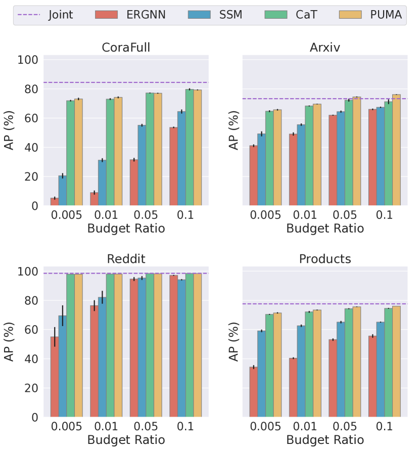
Figure 3: AP of different memory banks with different budget ratios. All memory banks use both TiM and retraining to obtain the best performance for fairness.

5.4.1 Different Memory Banks

Fig. 3 demonstrates that the PUMA is more effective than existing sampling-based memory banks. PUMA converges to optimal performance much quicker. PUMA gets the best performance in all evaluated cases. PUMA significantly outperforms other sampling-based memory banks when the budget ratio is relatively small (e.g., 0.005, 0.01). Besides, condensation-based memory banks have small standard errors at the limited memory budgets, demonstrating the robustness.

5.4.2 Budget Efficiency

The advantage of the condensed graph is to keep the information of the original graph while reducing the graph size significantly. Fig. 3 shows that the CaT and PUMA outperform the sampling-based methods in achieving higher performance within a more limited budget. In all datasets, the sampling-based methods have a huge performance gap to condensation-based methods. For example, PUMA with 0.005-budget ratio can outperform or match the 0.1-budget ratio sampling-based methods on CoraFull, Reddit and Products.

On the one hand, CaT and PUMA use less memory spaces to accurately approximate the historical data distribution. On the other hand, in the training phase, the model needs to propagate messages in the memory bank. Therefore, a small memory bank can improve both storage and computation efficiency.

5.5 Balanced Learning with TiM

5.5.1 Different Methods with TiM

TiM is a plug-and-play training scheme for all existing replay-based CGL methods. Table  V shows the mAP for different replay-based CGL methods with and without TiM. It clearly shows that the TiM scheme can improve the overall average performance with all memory bank generation methods. The reason is that the TiM can ensure training graphs for the CGL models have a similar size to deal with the imbalanced issue, which can solve the catastrophic forgetting problem.

TABLE V: Comparison of mAP (%) for replay-based CGL methods without and with TiM.

Method	TiM	CoraFull	Arxiv	Reddit	Products
ER-GNN	✗	11.3±0.0	37.6±0.6	50.9±1.9	37.1±0.6
	✓	13.8±0.7	56.5±1.1	77.5±1.0	42.0±0.5
SSM	✗	11.7±0.2	40.6±1.1	70.2±0.9	62.1±0.3
	✓	27.5±3.5	62.8±1.4	77.3±3.3	75.9±0.4
CaT	✗	29.2±1.4	44.1±1.2	89.4±0.7	72.7±0.2
	✓	76.7±0.6	74.0±0.4	98.7±0.0	83.7±0.2
PUMA	✗	70.6±0.5	57.7±0.4	97.6±0.0	72.1±0.1
	✓	80.6±0.5	75.7±0.3	98.7±0.0	84.3±0.2

5.5.2 Visualisation

The performance matrices of ER-GNN, SSM, CGM, and those memory banks training with TiM (i.e., EaT, SaT can CaT) on the CoraFull, Arxiv, Reddit and Products datasets under 0.01 budget ratio are visualised in Fig. 4. All memory banks without TiM struggle with remembering the previous knowledge since the scale gap between the newly incoming graph and replayed graphs in the memory bank. After using the TiM scheme, the performance matrices show the forgetting process slows down (i.e., the colour of each column is not changed a lot), which indicates the catastrophic forgetting problem is alleviated as the imbalanced training issue is tackled.

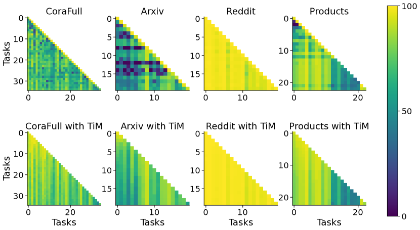
Figure 4: Performance matrix visualisation of PUMA with and without TiM scheme in all four datasets. The coloured square located at the $i_{th}$ row and the $j_{th}$ column denotes the classification accuracy of Task $\mathcal{T}_{j}$ after model training on Task $\mathcal{T}_{i}$. Light colour means high accuracy, and dark colour means low accuracy. The $i_{th}$ column from top to bottom can represent the accuracy changes during the model’s continual training of Task $\mathcal{T}_{i}$.

5.6 Effectiveness of Retraining

Although TiM effectively mitigates the issue of class training sample imbalance, it introduces a new challenge during continual training: imbalance in task losses. This occurs because memories added earlier to the memory bank have been sufficiently learned, resulting in smaller losses compared to those added later. For alleviating this problem, retraining strategy is proposed to train the CGL model in the memories from scratch. This section will discuss the effectiveness of retraining strategy by applying it to different memory banks.

TABLE VI: Comparison of mAP (%) for replay-based CGL methods without and with retraining.

Method	Re	CoraFull	Arxiv	Reddit	Products
ER-GNN	✗	13.8±0.7	56.5±1.1	77.5±1.0	42.0±0.5
	✓	16.1±0.5	58.7±0.8	81.1±3.1	43.9±0.7
SSM	✗	27.5±3.5	62.8±1.4	77.3±3.3	75.9±0.4
	✓	38.6±4.7	64.6±1.3	83.6±4.3	76.4±0.3
CaT	✗	76.7±0.6	74.0±0.4	98.7±0.0	83.7±0.2
	✓	83.6±0.5	75.4±0.3	98.9±0.0	84.2±0.2
PUMA	✗	80.6±0.5	75.7±0.3	98.7±0.0	84.3±0.2
	✓	84.4±0.5	76.4±0.3	98.9±0.0	84.6±0.1

5.6.1 Effectiveness

Table VI represents the mAP of different replay-based methods without and with retraining. The metric mAP is selected for comparative analysis, as it enables a comprehensive evaluation of accuracy at each step of the continual learning process, rather than focusing solely on the final step performance.

In the presented data, the efficacy of retraining in enhancing the performance of replay-based CGL methods is clearly demonstrated across various datasets. In the context of continual training, this aspect predisposes the model to overfitting on previous memories. Furthermore, the issue of imbalanced loss exacerbates this tendency, as it hinders the model’s ability to effectively learn the decision boundaries between newly added memories and historical ones. Consequently, retraining becomes crucial in this scenario, as it helps in recalibrating the model’s knowledge and adaptability to both new and existing data, thereby improving its overall performance.

5.6.2 Visualisation

Fig. 5 shows the accuracy changes of the fist task after receiving the last task of the graph streaming during continual training. For the CoraFull, Arxiv and Products datasets, the accuracy without retraining has a shake and converge then. Although the retrained model needs more steps to converge, the accuracy with retraining can outperform the continual training. For the Reddit dataset, retrain the CGL model cannot benefit a lot since the model accuracy is already high.

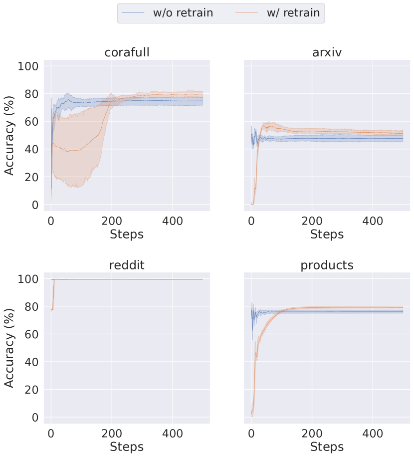
Figure 5: The accuracy (%) changes of the first task during continual training of the last task on CoraFull, Arxiv, Reddit, and Products datasets.

5.7 Condense More by Pseudo-Labelling

The impact of pseudo-labelling on the accuracy of replay-based CGL methods, such as ER-GNN, SSM, CaT and PUMA, is evaluated in this study. The comparison involves scenarios with and without the integration of pseudo labels during the memorisation stage. Table VII presents the mAP for different CGL methods under both conditions.

It is observed that for condensation-based graph memory, incorporating pseudo-labeling proves to be effective. This approach aids in training a robust classifier, which in turn generates useful pseudo-labels. Additionally, introducing pseudo labels into incoming graphs expands the training dataset, providing a more comprehensive set of supervisory signals. Such an expansion significantly enhances the generalisation capabilities of the CGL model, leading to improved accuracy in inferring labels of test nodes.

However, it is noted that the pseudo-labelling technique does not yield similar benefits for current sampling-based memory banks. The limitation primarily arises due to the reliance of pseudo-labelling classifiers on memory banks for training. Sampling-based memory banks with limited budgets might not contain sufficient information, which hampers the development of an effective classifier. On the other hand, the fixed budgets of sampling-based memory banks restrict their ability to add more information. This is in contrast to condensation-based methods, which can incorporate additional information despite similar budget constraints by discovering more unlabelled nodes.

TABLE VII: mAP of replay-based CGL methods with and without pseudo-labelling

Method	PL	CoraFull	Arxiv	Reddit	Products
ER-GNN	✗	11.3±0.4	51.6±1.0	67.6±3.7	36.2±1.7
	✓	11.2±0.5	50.1±0.4	68.7±2.7	34.5±0.8
SSM	✗	28.0±3.5	58.2±1.7	75.2±6.9	72.5±0.5
	✓	25.4±4.9	55.3±1.8	75.0±4.1	71.1±0.4
PUMA	✗	82.8±0.7	74.1±0.1	98.9±0.0	84.1±0.0
	✓	84.1±0.6	74.7±0.3	98.9±0.0	84.6±0.0

5.8 Wide Graph Encoder

A wide graph encoder includes more neurons with random initialised weights which randomly extracts features with non-linearity. Fig. 6 shows reducing the distance between original and condensed graph embeddings generated by a narrow encoders is not sufficient since there is still a clear distribution gap between them once the encoder is reinitialised. This gap is decreased by wider graph encoders.

The more neurons that can be obtained at one time, the clearer the potential transformations of the original data in the initialisation space will be, and the easier it will be for fitting the distribution of data through different networks. It is necessary to have an accurate distribution of data because in continual learning, new classes emerge continuously, and during the replay process, the model needs to relearn the decision boundary between different classes. However, more neurons spends more computation resources, multiple random encoders are used in practice.

800-dim embeddings	12800-dim embeddings

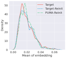
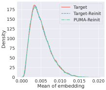
Figure 6: Kernel density estimation (KDE) plot of mean embeddings. It compares KDE of mean embeddings at different stages: ‘Target’ (original graph’s embedding), ‘Target-Reinit’ (original graph’s embedding by a reinitialised encoder), and ‘PUMA-Reinit’ (condensed graph’s embedding by a reinitialised encoder). The encoder dimensions of left figure and right figure are 800 and 12800 respectively.

5.9 Parameter Sensitivity

There are several hyperparameters in condensed memory bank generation, including the budget ratio for the replayed graph, which is already evaluated in Fig. 3. This section will discuss the choices of dimension of graph encoders and usage of activation during encoding.

5.9.1 Different Dimensional Graph Encoders

This experiment explores the sufficient dimensions of graph encoders to optimise the MMD loss. The condense iterations remain 500, and the graph encoder only randomly initialise once before condensation. Table 7 shows the AP (%) of the model trained by the PUMA generated by various dimensional graph encoders after handling each incoming task during the continual learning process.

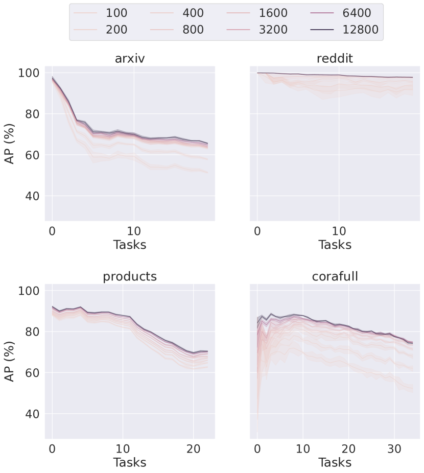
Figure 7: The average performance (AP) changes in the whole continual learning process with memory banks generated by different dimensional graph encoders. Except for CoraFull dataset, all other datasets only update the condensed graph 500 times under only one random parameterised graph encoder. For CoraFull, 50 random graph encoders are used to update the condensed graph 100 times individually for reducing the distribution distance in a larger embedding space since CoraFull’s 8710-dimensional features imply a larger model parameter initialisation space.

When the encoder dimensions are restricted because of the limited computational resources, model performance decreases since the model’s parameter initialisation space is not complete. As the dimension of the graph encoder increases, the CGL model’s performance experiences a significant improvement. It shows that for better covering the initialisation space of model parameters, wide encoders are essential. When the computation resources are limit, use more random relative small graph encoders can also get matching performance but need more condensation time.

5.9.2 Neuron Activation

This experiment will compare the use of activation functions in encoders for graph encoding. The standard node classification for CGL will still utilise an encoder with an activation function. mAP is employed to measure effectiveness. Table VIII illustrates that for varying budget ratios, encoders with activation functions are more competitive options for encoding graphs overall.

TABLE VIII: mAP (%) of different graph encoders with varying budget ratios

Activation	CoraFull
	0.005	0.01	0.05	0.1
✗	86.4±0.0	58.4±0.3	84.4±0.4	86.6±0.2
✓	84.1±0.6	74.5±0.4	85.7±0.1	86.6±0.1

Activation	Arxiv
	0.005	0.01	0.05	0.1
✗	71.4±0.5	73.8±0.2	76.7±0.3	77.6±0.2
✓	74.7±0.3	76.5±0.2	79.8±0.1	81.0±0.1

Activation	Reddit
	0.005	0.01	0.05	0.1
✗	98.8±0.0	98.8±0.0	98.9±0.0	98.9±0.0
✓	98.9±0.0	99.0±0.0	99.2±0.0	99.2±0.0

Activation	Products
	0.005	0.01	0.05	0.1
✗	79.2±0.3	80.8±0.1	83.8±0.2	85.0±0.1
✓	84.6±0.0	85.8±0.1	87.6±0.1	88.1±0.0

5.10 Time Efficiency

For replay-based CGL methods, memory generation and model training are two main parts for requiring computation resources. Fig. 8 compares the total time (memorisation plus training time) for ER-GNN, SSM, CaT and PUMA methods. Experiments are ran on CoraFull and Products datasets.

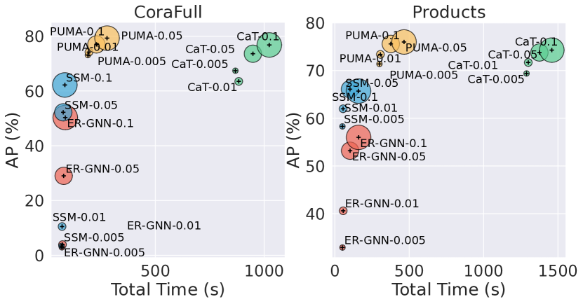
Figure 8: Total time (i.e., memorisation time plus training time) for different replay-based CGL methods in the streaming of Arxiv and Products datasets. x-axis represents total time (s) and y-axis indicates the AP (%). The size of scatter implies the budget of the memory bank.

For sampling-based methods (e.g., ER-GNN and SSM), memory generation process is efficient. Although the time of graph condensation cannot be ignored as sampling-based methods, the model accuracy are much better than sampling-based methods. For CaT, the main computation cost for the memory generation is the feature aggregation in the original graph. Since the condensed graph is significantly smaller than the original graph, the time of feature aggregation in the condensed graph can be ignored. Because the original graph is fixed, once the original graph’s aggregated features are obtained, it can be stored in the memory for reduce the repeatedly computation. Once weights of the graph encoder is reinitialised, the embedding of original graph in this embedding space is needed to recalculate. This step can be reduced by increasing the dimension of graph encoders, and it can even be reduced to 1 when the dimension of graph encoder is sufficient.

The memory bank of PUMA is edge-free, the feature aggregation operation in the training phase can be ignored, weights of each layer can be learned by a MLP model. The performance of PUMA can match the Joint method, but the operation time is faster.

Although edge-free condensed graph can accelerate the training process, it can not counteract the increasing time in the memory generation process. Considering the accuracy improvement of PUMA, it is still competitive.

6 Conclusion

This paper proposes a novel pseudo-label guided memory bank (PUMA) method for the CGL problem extending from our CaT [1] framework. PUMA enhances the efficacy of condensed graphs by using unlabelled nodes with pseudo labels to leverage more information from the unlabelled nodes. The condensation process efficiency is significantly improved due to one-time propagation and wide graph encoders. Despite balanced sizes in replayed graphs, an imbalance in training losses between existing and new memories is observed, while PUMA addresses this through a retraining strategy. Additionally, PUMA maintains an edge-free memory bank and trains a MLP model for mitigating the costly neighbour message aggregation. In conclusion, PUMA achieves state-of-the-art performance in numerous experiments while maintaining efficiency.

Yilun Liu completed his B.E degree at Griffith University in 2020, and M.I.T degree at The University of Queensland in 2022. Currently, he is a PhD student at the School of Electrical Engineering and Computer Science, the University of Queensland. His research interests include graph representation learning, dataset condensation and continual learning.

Ruihong Qiu is currently a Postdoctoral Research Fellow at The University of Queensland. He received his PhD degree in Computer Science at The University of Queensland in 2022. His research mainly focuses on recommender systems, graph neural networks, and data science for cross-disciplinary projects.

Yanran Tang is currently a PhD student at the School of Electrical Engineering and Computer Science, The University of Queensland. She holds an LLB and an LLM degrees. Her research interests include information retrieval and graph representation learning in legal domain.

Hongzhi Yin received his PhD degree in computer science from Peking University, in 2014. He is a professor and ARC Future Fellow with The University of Queensland. He received the Australian Research Council Discovery Early Career Researcher Award in 2016 and UQ Foundation Research Excellence Award in 2019. His research interests include recommendation system, user profiling, topic models, deep learning, social media mining, and location-based services.

Zi Huang received her BSc degree from Tsinghua University in 2001 and her PhD degree in computer science from The University of Queensland (UQ) in 2007. She is a professor and the Discipline Lead for Data Science at the School of Electrical Engineering and Computer Science, UQ. Her research interests mainly include multimedia, computer vision, social data analysis and knowledge discovery. She is currently an associate editor of The VLDB Journal, ACM Transactions on Information Systems (TOIS), etc and also a member of the VLDB Endowment Board of Trustees.

References

- [1] Y. Liu, R. Qiu, and Z. Huang, “Cat: Balanced continual graph learning with graph condensation,” in ICDM, 2023.
- [2] Q. Guo, F. Zhuang, C. Qin, H. Zhu, X. Xie, H. Xiong, and Q. He, “A survey on knowledge graph-based recommender systems,” TKDE, 2022.
- [3] P. Xie, M. Ma, T. Li, S. Ji, S. Du, Z. Yu, and J. Zhang, “Spatio-temporal dynamic graph relation learning for urban metro flow prediction,” TKDE, 2023.
- [4] L. Zhang, Y. Jiang, and Y. Yang, “Gnngo3d: Protein function prediction based on 3d structure and functional hierarchy learning,” TKDE, 2023.
- [5] Y. Xu, Y. Zhang, W. Guo, H. Guo, R. Tang, and M. Coates, “Graphsail: Graph structure aware incremental learning for recommender systems,” in CIKM, 2020.
- [6] A. A. Daruna, M. Gupta, M. Sridharan, and S. Chernova, “Continual learning of knowledge graph embeddings,” IEEE Robotics Autom. Lett., 2021.
- [7] R. Qiu, H. Yin, Z. Huang, and T. Chen, “GAG: global attributed graph neural network for streaming session-based recommendation,” in SIGIR, 2020.
- [8] F. Zhou and C. Cao, “Overcoming catastrophic forgetting in graph neural networks with experience replay,” in AAAI, 2021.
- [9] H. Liu, Y. Yang, and X. Wang, “Overcoming catastrophic forgetting in graph neural networks,” in AAAI, 2021.
- [10] X. Zhang, D. Song, and D. Tao, “Sparsified subgraph memory for continual graph representation learning,” in ICDM, 2022.
- [11] X. Zhang, D. Song, and D. Tao, “Hierarchical prototype networks for continual graph representation learning,” TPAMI, 2023.
- [12] R. Geirhos, J.-H. Jacobsen, C. Michaelis, R. Zemel, W. Brendel, M. Bethge, and F. A. Wichmann, “Shortcut learning in deep neural networks,” Nature Machine Intelligence, 2020.
- [13] K. Xu, W. Hu, J. Leskovec, and S. Jegelka, “How powerful are graph neural networks?” in ICLR, 2019.
- [14] Y. Li, D. Tarlow, M. Brockschmidt, and R. S. Zemel, “Gated graph sequence neural networks,” in ICLR, 2016.
- [15] Y. Tang, R. Qiu, Y. Liu, X. Li, and Z. Huang, “Casegnn: Graph neural networks for legal case retrieval with text-attributed graphs,” ECIR, 2024.
- [16] R. Qiu, Z. Huang, J. Li, and H. Yin, “Exploiting cross-session information for session-based recommendation with graph neural networks,” TOIS, 2020.
- [17] T. N. Kipf and M. Welling, “Semi-supervised classification with graph convolutional networks,” in ICLR, 2017.
- [18] P. Velickovic, G. Cucurull, A. Casanova, A. Romero, P. Liò, and Y. Bengio, “Graph attention networks,” in ICLR, 2018.
- [19] A. Vaswani, N. Shazeer, N. Parmar, J. Uszkoreit, L. Jones, A. N. Gomez, L. Kaiser, and I. Polosukhin, “Attention is all you need,” in NeurIPS, 2017.
- [20] F. Wu, A. H. S. Jr., T. Zhang, C. Fifty, T. Yu, and K. Q. Weinberger, “Simplifying graph convolutional networks,” in ICML, 2019.
- [21] W. L. Hamilton, Z. Ying, and J. Leskovec, “Inductive representation learning on large graphs,” in NeurIPS, 2017.
- [22] J. Kirkpatrick, R. Pascanu, N. C. Rabinowitz, J. Veness, G. Desjardins, A. A. Rusu, K. Milan, J. Quan, T. Ramalho, A. Grabska-Barwinska, D. Hassabis, C. Clopath, D. Kumaran, and R. Hadsell, “Overcoming catastrophic forgetting in neural networks,” CoRR, vol. abs/1612.00796, 2016.
- [23] R. Aljundi, F. Babiloni, M. Elhoseiny, M. Rohrbach, and T. Tuytelaars, “Memory aware synapses: Learning what (not) to forget,” in ECCV, 2018.
- [24] D. Lopez-Paz and M. Ranzato, “Gradient episodic memory for continual learning,” in NeurIPS, 2017.
- [25] Z. Li and D. Hoiem, “Learning without forgetting,” TPAMI, 2018.
- [26] X. Zhang, D. Song, and D. Tao, “Ricci curvature-based graph sparsification for continual graph representation learning,” TNNLS, 2023.
- [27] J. Su, D. Zou, Z. Zhang, and C. Wu, “Towards robust graph incremental learning on evolving graphs,” in ICML, 2023.
- [28] X. Zhang, D. Song, and D. Tao, “Cglb: Benchmark tasks for continual graph learning,” in NeurIPS Systems Datasets and Benchmarks Track, 2022.
- [29] J. Ko, S. Kang, and K. Shin, “Begin: Extensive benchmark scenarios and an easy-to-use framework for graph continual learning,” CoRR, vol. abs/2211.14568, 2022.
- [30] T. Wang, J. Zhu, A. Torralba, and A. A. Efros, “Dataset distillation,” CoRR, vol. abs/1811.10959, 2018.
- [31] B. Zhao, K. R. Mopuri, and H. Bilen, “Dataset condensation with gradient matching,” in ICLR, 2021.
- [32] B. Zhao and H. Bilen, “Dataset condensation with differentiable siamese augmentation,” in ICML, 2021.
- [33] K. Wang, B. Zhao, X. Peng, Z. Zhu, S. Yang, S. Wang, G. Huang, H. Bilen, X. Wang, and Y. You, “CAFE: learning to condense dataset by aligning features,” in CVPR, 2022.
- [34] B. Zhao and H. Bilen, “Dataset condensation with distribution matching,” in WACV, 2023.
- [35] G. Cazenavette, T. Wang, A. Torralba, A. A. Efros, and J. Zhu, “Generalizing dataset distillation via deep generative prior,” in CVPR, 2023.
- [36] W. Jin, L. Zhao, S. Zhang, Y. Liu, J. Tang, and N. Shah, “Graph condensation for graph neural networks,” in ICLR, 2022.
- [37] W. Jin, X. Tang, H. Jiang, Z. Li, D. Zhang, J. Tang, and B. Yin, “Condensing graphs via one-step gradient matching,” in KDD, 2022.
- [38] X. Gao, T. Chen, Y. Zang, W. Zhang, Q. V. H. Nguyen, K. Zheng, and H. Yin, “Graph condensation for inductive node representation learning,” ICDE, 2024.
- [39] Y. Chen, M. Welling, and A. J. Smola, “Super-samples from kernel herding,” in UAI, 2010.
- [40] Z. Wang and J. Ye, “Querying discriminative and representative samples for batch mode active learning,” in KDD, 2013.
- [41] O. Sener and S. Savarese, “Active learning for convolutional neural networks: A core-set approach,” in ICLR, 2018.
- [42] M. Liu, S. Li, X. Chen, and L. Song, “Graph condensation via receptive field distribution matching,” CoRR, vol. abs/2206.13697, 2022.
- [43] X. Zheng, M. Zhang, C. Chen, Q. V. H. Nguyen, X. Zhu, and S. Pan, “Structure-free graph condensation: From large-scale graphs to condensed graph-free data,” NeurIPS, 2023.
- [44] B. Yang, K. Wang, Q. Sun, C. Ji, X. Fu, H. Tang, Y. You, and J. Li, “Does graph distillation see like vision dataset counterpart?” NeurIPS, 2024.
- [45] W. Masarczyk and I. Tautkute, “Reducing catastrophic forgetting with learning on synthetic data,” in CVPR Workshop, 2020.
- [46] F. Wiewel and B. Yang, “Condensed composite memory continual learning,” in IJCNN, 2021.
- [47] A. Rosasco, A. Carta, A. Cossu, V. Lomonaco, and D. Bacciu, “Distilled replay: Overcoming forgetting through synthetic samples,” in CSSL Workshop, 2021.
- [48] M. Sangermano, A. Carta, A. Cossu, and D. Bacciu, “Sample condensation in online continual learning,” in IJCNN, 2022.
- [49] J. Gu, K. Wang, W. Jiang, and Y. You, “Summarizing stream data for memory-restricted online continual learning,” CoRR, vol. abs/2305.16645, 2023.
- [50] H. Han, X. Liu, H. Mao, M. Torkamani, F. Shi, V. Lee, and J. Tang, “Alternately optimized graph neural networks,” in ICML, 2023.
- [51] D.-H. Lee et al., “Pseudo-label: The simple and efficient semi-supervised learning method for deep neural networks,” in ICML Workshop, 2013.
- [52] A. McCallum, K. Nigam, J. Rennie, and K. Seymore, “Automating the construction of internet portals with machine learning,” Inf. Retr., 2000.
- [53] W. Hu, M. Fey, M. Zitnik, Y. Dong, H. Ren, B. Liu, M. Catasta, and J. Leskovec, “Open graph benchmark: Datasets for machine learning on graphs,” in NeurIPS, 2020.
- [54] D. Zhou, Q. Wang, Z. Qi, H. Ye, D. Zhan, and Z. Liu, “Deep class-incremental learning: A survey,” CoRR, vol. abs/2302.03648, 2023.
- [55] L. Wang, X. Zhang, H. Su, and J. Zhu, “A comprehensive survey of continual learning: Theory, method and application,” CoRR, vol. abs/2302.00487, 2023.