remarkRemark \newsiamremarkhypothesisHypothesis \newsiamthmCorollaryCorollary \newsiamthmDefinitionDefinition \newsiamthmAssumptionAssumption \headersTime-inconsistent mean field and n-agent gamesZongxia Liang and Keyu Zhang
Time-inconsistent mean field and n-agent games under relative performance criteria††thanks: Submitted to the editors November 11, 2022. \fundingThis work was funded by the National Natural Science Foundation of China, grants 12271290 and 11871036.
Abstract
In this paper we study a time-inconsistent portfolio optimization problem for competitive agents with CARA utilities and non-exponential discounting. The utility of each agent depends on her own wealth and consumption as well as the relative wealth and consumption to her competitors. Due to the presence of a non-exponential discount factor, each agent’s optimal strategy becomes time-inconsistent. In order to resolve time-inconsistency, each agent makes a decision in a sophisticated way, choosing open-loop equilibrium strategy in response to the strategies of all the other agents. We construct explicit solutions for the -agent games and the corresponding mean field games (MFGs) where the limit of former yields the latter. This solution is unique in a special class of equilibria. As a by-product, we find that competition in the time-inconsistency scenario modifies the agent’s risk tolerance as it does in the time-consistent scenario.
keywords:
relative performance, mean field games, time-inconsistency, open-loop equilibrium, forward backward stochastic differential equation91A06, 91A07, 91A16, 91B51
1 Introduction
Due to the fact that peer interaction sometimes makes remarkable impacts on agent’s decision making, portfolio games, as a game-theoretic extension of classical Merton problem [28], have received considerable attention in recent years. Relative performance is becoming an appealing way to model the interaction because of the tractability in mathematics and excellent economic motivations. The literature on portfolio games with relative performance concerns dates by to Espinosa and Touzi [16], where they consider -agent games with portfolio constrains under the CARA utility by investigating the associated quadratic BSDEs systems. Lacker and Zariphopoulo [24] consider the portfolio games for asset specialized agents in log-normal markets under both CARA and CRRA relative performance criteria. The constant Nash equilibrium and mean field equilibrium (MFE) are explicitly constructed. In a similar fashion, Lacker and Soret [23] extend the problem by incorporating the dynamic consumption. Bo et al. [7] revisit the MFGs and the -agent games under CRRA relative performance by allowing risky assets to have contagious jumps. A deterministic MFE in an analytical form is obtained by using the FBSDE and stochastic maximum principle. Furthermore, an approximate Nash equilibrium for the -agent games is constructed. Recently, Fu and Zhu [18] study the mean field portfolio games with general market parameters. A one-to-one correspondence between the Nash equilibrium and the solution to some FBSDE is established by martingale optimality principle.
Another research direction with fruitful outcomes is time-inconsistent control problem, where the Bellman optimality principle does not hold. There are many important problems in mathematical finance and economics incurring time-inconsistency, for example, the mean-variance selection problem and the investment-consumption problem with non-exponential discounting. The main approaches to handle time-inconsistency are to search for, instead of optimal strategies, time-consistent equilibrium strategies within a game-theoretic framework. Ekeland and Lazrak [14] and Ekeland and Pirvu [15] introduce the precise definition of the equilibrium strategy in continuous-time setting for the first time. Björk et al. [5] derive an extended HJB equation to determine the equilibrium strategy in a Markovian setting. Yong [31] introduces the so-called equilibrium HJB equation to construct the equilibrium strategy in a multi-person differential game framework with a hierarchical structure. The solution concepts considered in [5, 31] are closed-loop equilibrium strategies and the methods to handle time-inconsistency are extensions of the classical dynamic programming approaches. In contrast to the aforementioned literature, Hu et al. [21] introduce the concept of open-loop equilibrium control by using a spike variation formulation, which is different from the closed-loop equilibrium concepts. The open-loop equilibrium control is characterized by a flow of FBSDEs, which is deduced by a duality method in the spirit of Peng’s stochastic maximum principle. Some recent studies devoted to the open-loop equilibrium concept can be found in [2, 3, 30, 19]. Specially, Alia et al. [3], closely related to our paper, study a time-inconsistent investment-consumption problem under a general discount function, and obtain an explicit representation of the equilibrium strategies for some special utility functions, which is different from most of existing literature on the time-inconsistent investment-consumption problem, where the feedback equilibrium strategies are derived via several complicated nonlocal ODEs; see, e.g., [27, 6].
To the best of our knowledge, the -agent games and MFGs under relative performance when the non-exponential discounting is considered have not been studied before. The constant discount rate is a common assumption in classical portfolio management problems under discounted utility which suggests the discount function should be exponential. But results from experimental studies contradict this assumption, indicating that agents may be impatient in the face of choices in the short term but be patient when choosing between long-term alternatives; see, e.g., [1]. Therefore, it is interesting to investigate the non-exponential discounting case.
Our paper aims to contribute to the literature of the aforementioned -agent games and MFGs under relative performance by considering general discount functions. Specially, the discount function only needs to satisfy some weak conditions; see Remark 2.1 in Section 2. Meanwhile, we adopt the asset specialization framework in [24, 7] with a common noise. A lot of literature on equilibrium strategy under non-exponential discounting suggest that the investment strategy is independent of discount function, which indicates that time-inconsistency does not influence agent’s portfolio policy; see, e.g., [27, 6]. Thus instead of portfolio games, we incorporate consumption in the same spirit of [23] and focus on CARA relative performance utility. As opposed to the previous works, the presence of non-exponential discounting gives rise to time-inconsistency, which induces the failure of the principle of optimality. In order to resolve time-inconsistency, we replace each agent’s optimal strategy in time-consistent setting by its open-loop equilibrium (consistent) strategy in time-inconsistent setting. As a result, there are two levels of game-theoretic reasoning intertwined. (1) The intra-personal equilibrium among the agent’s current and future selves. (2) The equilibrium among -agents. For tractability, we search only for DF equilibrium strategy, a new definition we define for brevity (see Remark 2.3), which is comparable with the strong equilibrium in [23]. To construct the DF equilibrium strategy, we first characterize the open-loop consistent control for each single agent given an arbitrary (but fixed) choice of competitors’ controls by a FBSDE system. By assuming that all the other agents choose DF strategies (see Section 2), we derive a closed form representation of the strategy via a PDE system. We then construct the desired equilibrium by solving a fixed point problem. While for MFG, the solution technique is analogous to the -agent setting and the resulting MFE takes similar forms as its -agent counterparts.
The contributions of our paper are as follows: first, as far as we know, our work is the first paper to incorporate consumption into CARA portfolio game with relative performance concerns. In fact, portfolio games under relative consumption are poorly explored, except in [23], where they only focus on CRRA utilities under zero discount rate. Our paper fills the gap in the literature. Second, our work can be seen as a game-theoretic extension of the exponential utility case in [3]. In the special case of a single stock, the DF equilibrium strategy takes the same form with the open-loop equilibrium in [3] but with a modified risk tolerance. This effective risk tolerance parameter has already appeared in some works on a similar topic but with a time-consistent model; see, e.g., [24, 20]. Moreover, in the case with constant discount rate, the equilibrium reduces to the solution of classical Merton problem, which indicates that the equilibrium concept in our paper is the natural extension of equilibrium in classical time-consistent setting to time-inconsistent setting. Third, our work also provides a new explicitly solvable mean field game model. Since the pioneering works by [25, 22], MFGs have been actively studied and widely applied in economics, finance and engineering. To name a few recent developments in theories and application, we refer to [12, 8, 13, 9, 10] among others. However, few studies combine the MFGs with time-inconsistency problem, except some linear quadratic examples; see, e.g., [29, 4]. Our result adds a new explicitly solvable non-LQ example to intersection of these two fields.
The rest of paper is organized as follows. In Section 2, we formulate and solve the -agent games under CARA relative preference and a general discount function. Then, in Section 3, we study the infinite population counterpart of this problem, and identify resulting MFE agree with the limiting expressions from the -agent games. Section 4 presents some qualitative comments on the MFE. Some conclusion remarks and future research directions are given in Section 5. Finally, the proofs of some auxiliary results are in Appendix.
Notations. For any Euclidean space with norm , and any , denote
: the set of -valued -measurable random variables X, such that
: the space of -valued -adapted and continuous processes Y with
: the space of -valued -progressively measurable processes Z with
2 The -agent games
In this section, we consider the -agent games. The market model is same as [24] and each agent invests in their own specific stock or in a common riskless bond which offers zero interest rate. The common time horizon for all agents is with . The price process of stock , in which only agent trades, follows the following stochastic differential equation (SDE)
| (1) |
with constant parameters , , and with , where the Brownian motions and are independent on a filtered probability space , in which the natural filtration is generated by these Brownian motions.
We recall the single stock case, corresponding to the situation where , , and , for all and for some , independent of .
Each agent trades, using a self-financing strategy, , representing the amount invested in the stock , and a consumption policy, , representing the consumption rate of agent . Then the -th agent’s wealth process is
| (2) |
Now, we introduce the admissible control as follows. {Definition}[Admissible control]
A control is said to be admissible over if . For brevity, we denote as the set of all admissible controls over .
Then, for any , the state equation Eq. 2 has a unique solution . Moreover, we have the estimate:
for some constant .
We focus on the DF (deterministic-feedback) strategy defined as follows. {Definition}[DF strategy]
An -tuple of pairs is said to be a DF strategy, if for each , is a continuous function and is of an affine form:
for some continuous functions . We denote the set of DF strategies by . Moreover, a DF strategy is said to be simple if for every , the function does not depend on . Let a DF strategy be given. Then, for each initial condition with , we can solve the closed-loop system for :
| (3) |
Then, it is easy to see that the outcome defined by
| (4) |
is in , that is, an -tuple of admissible controls on .
Remark 2.1.
It is worth noting that the DF strategy does not depend on the initial condition , while the outcome depends on .
Let be given. For each initial condition , denote by and by the corresponding outcomes. Fix , and assume that a.s. for a.e. for every . Then it holds that and for any .
As we mention before, growing evidence suggests that the discount rate may not be constant, and in our work, we discuss the general discounting preferences.
[Discount Function]
A discount function is a continuous and strictly positive function satisfying .
Remark 2.2.
Definition 2.1 is general enough to cover some special discount functions, such as exponential discount functions (see, e.g., [28]), quasi-exponential discount functions (see, e.g., [15]) and hyperbolic discount functions (see, e.g., [33]). In fact, our result can be extended to a more general form of the discount factor as [19], where the discount function is a positive bivariate continuous function on satisfying , as the very thing we need is continuity of the discount function.
The utility function of the agent is defined as follows:
where and the constants and represent the personal risk tolerance and competition weight parameters, respectively. Note that the utility function also can be seen as a function of and :
Each agent derives a reward from their discounted inter-temporal consumption and final wealth, to be specific, for agent , the expected payoff is
| (5) |
defined for any admissible controls , where and .
For , we introduce the following notations:
It is well known that the optimal strategy of agent turns out to be time-inconsistent as soon as discounting is non-exponential. Hence, we assume that all agents are sophisticated, which means that they aim to find the best current action in response to their future selves’ behavior. When every future self also reasons in this way, the resulting strategy is an equilibrium form which no future self has any incentive to deviate.
As in [3, 21], we consider open-loop Nash equilibrium by local spike variation. For , any -valued, -measurable and bounded random variable , and any , given an admissible control , define
| (7) |
We have the following definition.
[Open-loop consistent control]
Let , and be given. An admissible control is said to be an open-loop consistent control for agent with respect to the initial wealth in response to if for every and every sequence such that , the following local optimality condition holds:
where and are defined by Eq. 2 and Eq. 6, respectively, with the initial wealth and the admissible controls , that is,
and
Remark 2.3.
We note that there is a slight difference between our definition and the classical definition of open-loop equilibrium given by [21]. If we adapt the classical definition in our problem, the open-loop consistent control should satisfy
where is an uncountable family of random variables and the a.s. limit as may not be well-defined. Hence, we avoid to use this definition in our problem.
The following technical integrability condition on an -tuple of admissible controls is needed to guarantee the uniqueness of the open-loop consistent control. For a deeper discussion on the uniqueness of the open-loop consistent control, we refer the reader to [19]. {Assumption}[Integrability condition]
Let be given. An -tuple of admissible controls satisfies the integrability condition if
where and are defined by Eq. 2 and Eq. 6, respectively, with the initial wealth and the admissible controls .
Now, we are ready for the following definitions. {Definition}[Open-loop equilibrium control]
Let be given. An -tuple of admissible controls is said to be an open-loop equilibrium control with respect to the initial wealth if for every , is an open-loop consistent control for agent with respect to the initial wealth in response to . {Definition} [DF equilibrium strategy]
A DF strategy is said to be a DF equilibrium strategy if for every , the corresponding outcome is an open-loop equilibrium control with respect to the initial wealth . Moreover, a DF equilibrium strategy is said to be simple if the DF strategy is simple.
Remark 2.4.
For the sake of brevity we use the name “equilibrium strategy” but it is different to “close-loop equilibrium strategies” or “subgame-perfect equilibrium strategies” discussed in the literature of time-inconsistent problems. A more appropriate name would be a “DF representation of open-loop equilibrium controls”.
The main result of this section is the following, which gives the explicit form of an equilibrium:
Theorem 2.5.
Assume that for all (), we have , , , , and . Then there exists a simple DF equilibrium strategy being the following form:
| (8) | |||
| (9) |
The constants and are
| (10) |
The function is
| (11) |
where
| (12) |
Furthermore, if we additionally assume that for all , then the obtained strategy is the unique simple DF equilibrium strategy.
It is straightforward to obtain the following corollary, which covers the single stock case. {Corollary}[Single stock] Assume that for all , we have , , and . Then the strategy has the following form:
| (13) |
where the function is
| (14) |
Remark 2.6.
A similar assumption on also appears in [16] and [17], which is mainly used to show the convergence from -agent games to MFGs. In the subsequent proof, we assume for all , so the reader can understand why we need this strange assumption in Theorem 2.5.
Proof 2.7 (Proof of Theorem 2.5).
Let and be given. We denote by a candidate control for agent . Assume that the inputs are of the following form:
where and is the wealth process associated with and satisfying
| (15) |
We now find the open-loop consistent control for agent in response to , then we resolve the resulting fixed point problem to obtain the desired equilibrium.
Open-loop consistent control for agent . According to Theorem A.3 in Appendix A, we first aim to find a classical solution of the following PDE:
| (16) |
Based on the terminal condition, we guess that the solution has the following form:
where , and such that , and .
Substituting the ansatz into Eq. 16, we obtain
Although the term in the last line depends on , we can solve the above equation correctly. Indeed, if and solve the following ODEs:
| (17) |
whose unique solutions are given by
| (18) |
then it holds that for any . Thus, the coefficient of vanishes, and we obtain the ODE of :
with terminal condition , whose solution is given by
| (19) |
where the deterministic function is defined by
for .
Then, by the representation of in Eq. 16, we have
| (20) |
In particular, does not depend on the state argument . It is clear that and does not depend on the initial wealth . By Lemma A.4 and Theorem A.3, we get that the outcome associated with is indeed an open-loop consistent control for agent with respect to the initial wealth in response to .
Fixed point problem. From the above discussion, we actually construct a best response map
| (21) |
by Eq. 20, which maps a DF strategy into a DF strategy. Now, we aim to find the fixed point of the map .
We first address the investment strategies. For a candidate portfolio vector to be the fixed point, we need , for and . Let
Then,
which yields
| (22) |
Multiplying both sides of Eq. 22 by and then averaging over , gives the following fixed point equation:
| (23) |
with as in Eq. 10.
We then have the following cases to get the fixed point:
- (i)
-
(ii)
If , then the equation Eq. 23 has no solution. Note that and cannot happen. Using assumption , , and , one can easily get a contradiction.
Next, we address the consumption strategies. Similarly, in order to be the fixed point, the candidate consumption vector needs to satisfy , for and . Let
The equation Eq. 24 implies
| (25) |
Averaging over , gives
| (26) |
where represents the arithmetic mean.
Then, we have the following cases to get the fixed point:
- (i)
-
(ii)
If and , then equation Eq. 26 has no solution.
-
(iii)
If and , then there exist infinitely many solutions.
In order to remove ‘bad’ cases, we limit in for all . In summary, we get that there exists a unique solution to the fixed point problem, which turns out to be a simple DF equilibrium strategy given by Eq. 8 and Eq. 9.
Uniqueness. To prove the uniqueness argument, we additionally assume that for all . We claim that a simple DF equilibrium strategy is equivalent to a fixed point of the map . Indeed, by the above discussion, we get that the fixed point of must be a simple DF equilibrium strategy. It remains to show that a simple DF equilibrium strategy must be a fixed point of .
Assume that is a simple DF equilibrium strategy. Define
Then, for each , we consider the controls and determined by
where and are defined by
and
It is clear that and hold for every . By the construction of controls and , we have that for each ,
is the open-loop consistent control for agent with respect to the initial wealth in response to ;
is the open-loop consistent control for agent with respect to the initial wealth in response to .
Since the inputs, and , are same and both and satisfy the Remark 2.3 according to the Lemma A.4, we can deduce that holds for every by the uniqueness of the open-loop consistent control, see [19]. Hence, we have for every . In this case, we have and . We claim that does not depend on and for any .
Indeed, we state that in this case if there exists an -tuple of pairs of a continuous function such that
then there must be for every and .
Assume that for each , has the following represetation:
where and are continuous functions of . Then we can explicitly derive : for every ,
where is given by Eq. 8 and
For a given , if
or equivalently,
then
| (27) | |||
| (28) | |||
| (29) |
where Eq. 28 is also equivalent to
Hence, the assumption for all deduces for all . By the arbitrariness of and the continuity of functions , it can be concluded that holds for every and .
Therefore, is a fixed point of . As has a unique fixed point, we have proved the uniqueness of the simple DF equilibrium strategy.
Remark 2.8.
We revisit the infinitely many solutions case of the fixed point problem. The discount function can be obtained by solving the following equations,
By calculation, we get
which is equivalent to the following ODE,
where , and . Then, one can get that the discount function is . If we relax the assumption on in Theorem 2.5 and further assume that for all , we have that
- (i)
-
(ii)
If and , then there exist infinitely many DF equilibrium strategies.
-
(iii)
If and , then no simple DF equilibrium strategy exists.
3 The mean field game
In this section, we investigate the limit as of the -agent game discussed in Section 2.
First we will use a heuristic argument as [23, 24] do to build intuition. For the -agent games, we define, for each agent , the type vector
These type vectors induce an empirical measure, called the type distribution, which is the probability measure on the type space:
given by
We assume that converges to some limiting probability measure , in order to pass to the limit, let us denote a -valued random variable with distribution , then we should expect the strategy to converge to
| (30) |
where
and
| (31) |
The function is
| (32) |
where
| (33) |
and is denoted as its randomization. In this section, we always assume , where is an arbitrary Borel measurable function. We explain that this strong assumption is needed to construct the best response map from DF strategies (see Section 3) to DF strategies (see the proof of Theorem 3.1). If one only wants to verify that the obtained strategy is a DF equilibrium strategy (see Section 3), it is enough to assume all the expectations in the aforementioned discussion are finite.
We next explain how this strategy arises as the equilibrium of the MFG. Now, we assume that the filtered probability space supports independent Brownian motions and , as well as random type vector independent of and , and with values in the space , where is the minimal filtration satisfying the usual assumptions such that is -measurable and both and are - Brownian motions. Let also denote the natural filtration generated by the Brownian motion .
Then the representative agent’s wealth process is determined by
| (34) |
As before, we give the definition of admissible control and DF strategy in the framework of MFG. {Definition}[Admissible control]
A control is said to be admissible over , if is an -progressively measurable process and for any given deterministic sample ,
For brevity, we denote as the set of all admissible controls over . {Definition}[DF strategy]
A pair is said to be a DF strategy, if and are of the following forms:
where is a positive integer, , and are Borel measurable functions, and , are continuous functions. Moreover, for any , and are continuous functions; and are also continuous. We denote the set of DF strategies by . Similarly, a DF strategy is said to be simple if does not depend on .
Now we formulate the representative agent’s optimization problem. Note that this is a mean field game with common noise , so conditional expectations given will be involved. As argued in [11, 23], conditionally on the Brownian motion B, we can get some kind of law of large numbers and asymptotic independence between the agents as , which suggests that the average wealth and consumption should be -adapted processes. Then, the expected payoff of the representative agent is
| (35) |
where is a discount function defined in Remark 2.1 and . The objective of the representative agent is to find the open-loop consistent control.
Similarly, we introduce the integrability condition as follows. {Assumption} [Integrability condition]
We say that an admissible control and average processes satisfy the integrability condition if for any deterministic sample , we have
where is defined by Eq. 34 with random type vector and the admissible control .
As the equilibrium should lead to and , we formalize this discussion in the following definition.
[Mean Field Equilibrium]
Let be an admissible control over , and consider the -adapted processes and , where is the wealth process corresponding to the control . We say that is a mean field equilibrium if is an open-loop consistent control corresponding to this choice of and for any deterministic sample .
A DF strategy is said to be a DF equilibrium strategy if the corresponding outcome is a mean field equilibrium. Moreover, a DF equilibrium strategy is said to be simple if the DF strategy is simple.
Theorem 3.1.
Assume that, a.s., , , , , , and . Define the constants
where we assume that both expectations are finite. Then there is a simple DF equilibrium strategy taking the following form:
| (36) | |||
| (37) |
where is the randomization of , given by
| (38) |
where
| (39) |
and we assume that all the expectations are finite. Furthermore, if we additionally assume that and , then the obtained strategy is the unique simple DF equilibrium strategy.
Similarly, we highlight the single stock case, noting that the form of the solution is essentially the same as in the -agent games, presented in Theorem 2.5. {Corollary}[Single stock] Suppose that are deterministic, with and . Then the strategy has the following form:
| (40) | |||
| (41) |
where the function is the same as Eq. 14.
Proof 3.2 (Proof of Theorem 3.1).
First, observe that it suffices to restrict our attention to stochastic processes and of the form and , where is defined by Eq. 34 with an admissible control . Moreover, we assume that is the outcome of a DF strategy :
| (42) |
where , , , and are defined in Section 3.
As , and are independent, then we have and the dynamic of is
| (43) |
We now find the open-loop consistent control for the representative agent, then we resolve the resulting fixed point problem to obtain the desired equilibrium.
Open-loop consistent control for the representative agent. Let represent a deterministic sample from its random type distribution for now. According to Theorem A.7 in Appendix A, we aim to find a classical solution of the following PDE:
| (44) |
We consider the following ansatz based on the terminal condition:
| (45) |
where and such that , and .
Putting Eq. 45 into Eq. 44, we have
If and solve the following ODEs:
| (46) |
which is explicitly solved by
| (47) |
then it holds that for any . Hence, we obtain the ODE for :
with the terminal condition , whose solution is given by
| (48) |
where
| (49) |
Then, by the representation of in Eq. 44, we have
| (50) |
Note that is independent of the state argument and . In the same manner as the -agent case, we obtain that for -type agent, the outcome associated with is an open-loop consistent control.
Thus, the open-loop consistent control for the representative agent is
| (51) | |||
| (52) | |||
where is defined by
Moreover, if we assume that all the expectations associated with the random type vector is finite, then we get that is also a DF strategy. Hence, we have constructed a best response map
| (53) |
Fixed point problem. We first address the investment strategies. Recalling the Section 3, we see that for the candidate investment strategy to be a fixed point, we need , for . In light of Eq. 51, we have
| (54) |
Multiply both sides of equation Eq. 54 by and average to find that must satisfy the following fixed point equation:
| (55) |
We then have the following cases to get the fixed point:
- (i)
-
(ii)
If , then the equation Eq. 55 has no solution. Note that and cannot happen. By assumption , , and , one can easily get a contradiction.
Next, we address the consumption strategies. Similarly, the candidate consumption strategy need to satisfy that
where . In fact, using the result in Appendix B, we have . To avoid confusion, we use instead of . Then we should solve the following fixed point problem:
| (56) |
Taking the conditional expectation given both sides of Eq. 56 to find that
| (57) |
then we have the following cases to find the fixed point:
- (i)
-
(ii)
If and , then equation Eq. 57 has no solution.
-
(iii)
If and , then there exist infinitely many solutions.
We limit in to remove ‘bad’ cases. In summary, we get that there exists a unique solution to the fixed point problem, which turns out to be a simple DF equilibrium strategy given by Eq. 36 and Eq. 37. Similar to the discussion on uniqueness in the proof of Theorem 2.5, we can also get that if we additionally assume that and , then is the unique simple DF equilibrium strategy.
Remark 3.3.
As the -agent games, by solving a similar ODE, the discount function in infinitely many fixed points case is . Similarly, if we relax the assumption on and further assume that and , we get that
- (i)
-
(ii)
If and , then there exist infinitely many DF equilibrium strategies.
-
(iii)
If and , then no simple DF equilibrium strategy exists.
4 Discussion of the equilibrium
We now discuss the interpretation of equilibria. We limit the discussion to the mean field case, for which the DF equilibrium strategy is given by Theorem 3.1 and Theorem 3.1, as -agent equilibria have essentially the same structure.
First, the investment strategy is -measurable and wealth independent, which means that if the agent gets richer, she will decrease the proportion of investment in the risky asset. Note that the investment strategy is independent of the discount function, which is consistent with the result of [3] and [27]. Moreover, consists of two components. The first, , is the classical Merton portfolio. The second component is always nonnegative, vanishing only when , which means no competition. It is clear that with increasing the competition weight , the agent will increase the allocation in the risky asset. Note that is a linear function of , and the coefficient is equal to the solution of the MFG in [24], where the consumption is not considered. Then it is obvious to see that as time goes on, the agent will invest less in the risky asset, and at terminal time , the amount invested in the risky asset drops down to the amount (equilibrium portfolio) in [24]. For more analysis of the influence of the parameters, we refer the reader to [24].
We further restrict our attention to the single stock case of Theorem 3.1, where the effects of the parameter are more transparent. Note that if , then we recover the open-loop equilibrium strategy without competition, with and ; see [3] for comparison. For the general , we may still rewrite and in an analogous manner as
where the effective risk tolerance parameter is
The parameter has already appeared in [24] and [20] and it is obvious to see that if , the difference increases with , with , and with .
We consider the following hyperbolic discount function,
where , . In particular, . In this case the DF equilibrium strategy reduces to the solution of Merton problem:
which is consistent with the fact that time-consistent equilibrium strategy under exponential discounting is nothing but the optimal strategy; see, e.g., [3, 6].
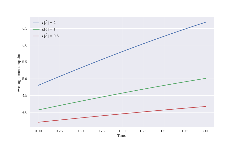
Finally, we numerically compute the average consumption . The parameters are , , and . As we can see in Fig. 1, the average consumption decreases with increasing . Note that a larger means that the agent is more patient in the future; see, e.g., [26]. We can either say that the difference between the agent and her future self is large when is large. In order to make an agreement, the sophisticated agent may give up more of her utility to the future. Hence, it is reasonable to spend less on consumption. In Fig. 2, we investigate the impact of competitiveness and risk tolerance on the average consumption. It is clear that the average consumption increases with increasing . Since increases when increases or increases, we conclude that in an environment with high competition or high risk tolerance, the average consumption is also high.

5 Conclusions and future research
We have studied the MFGs and the -agent games under CARA relative performance by allowing general discount functions. To deal with the time-inconsistency, each agent chooses the open-loop consistent control which is finally characterized by a PDE. By solving a fixed point problem, we explicitly constructed the DF equilibrium and the associate MFE. Next, we discuss some possible extensions for future research.
A natural extension is to consider CRRA utilities, which are also commonly used in models of portfolio choice. However, this extension is by no means straightforward. By introducing the non-exponential discount function into the model of [23], the verification method to characterize the open-loop consistent control used in our paper no longer works. A new approach needs to be developed. Another extension is to consider the closed-loop equilibrium strategy, in which the equilibrium strategy will be characterized by a system of nonlocal ODEs with complicated coupling structure. Both theoretical analysis and numerical solution will be a huge challenge. Finally, it will be interesting to extend our current work to a model with general market parameters, e.g., the incomplete market model considered in [19]. A closed form solution may not exist. The existence of an MFE may require some different mathematical arguments.
Appendix A The characterization of open-loop consistent control
A.1 The -agent games
In this section, we aim to characterize the open-loop consistent control by verification argument in the same spirit of [3]. Moreover, similar to classical time-consistent stochastic optimal control problem, we derive a PDE, which gives us a characterization of open-loop consistent control.
Let , and be given. We denote by a candidate control for agent and introduce the following BSDE defined on the interval :
| (58) |
where and are given by
and
If , then BSDE Eq. 58 has a unique solution
where .
Then we have the following theorem:
Theorem A.1.
Assume that . Then, the is an open-loop consistent control for agent with respect to the initial wealth in response to , if the following conditions hold
| (59) | |||
| (60) |
Proof A.2 (Proof of Theorem A.1).
Suppose that is an admissible control satisfies the conditions Eq. 59-Eq. 60. For any and , we consider by Eq. 7, then we have the following difference
Using the concavity and the terminal condition in BSDE Eq. 58, we obtain
| (61) |
Applying Ito’s formula,
| (62) |
Taking Eq. 62 in Eq. 61 yields
According to the conditions Eq. 59 and Eq. 60, we get
Now dividing both sides of the last inequality by and taking the limit, as is continuous, we conclude that is an open-loop consistent control for agent with respect to the initial wealth in response to .
Suppose that is an open-loop consistent control for agent with respect to the initial wealth in response to . In the view of Theorem A.1, we consider the following FBSDEs:
| (63) |
with conditions
| (64) | |||
| (65) |
It is hard to solve the above system due to the non-Markovianity of the inputs . Hence, we assume that the inputs are of the following form:
where and is the wealth process associated with and satisfying
| (66) |
Now, the constrained FBSDEs bocomes
| (67) |
with conditions
| (68) | |||
| (69) |
where
Based on the terminal condition of the BSDE Eq. 58, we consider the following ansatz:
| (70) |
for some deterministic function satisfying the following terminal condition:
Applying Ito’s formula to Eq. 70 yields
Comparing the above equation with the third equation in Eq. 67, we have
| (71) |
Then
| (72) | |||
| (73) |
Then, substituting the expressions Eq. 72 and Eq. 73 into the first equation of (71), we obtain the following verification theorem.
Theorem A.3.
Under the assumption of Theorem A.1, if there exists a classical solution of the following PDE:
| (74) |
and if the (-dimensional) SDE
| (75) |
has a solution such that the controls , , and are admissible over , then is an open-loop consistent control for agent with respect to the initial wealth in response to .
We stress that in order to prove that is an open-loop consistent control, one should verify the following conditions:
-
(i)
The SDE Eq. 75 has a solution;
-
(ii)
and .
The following lemma shows that if , then conditions (i) and (ii) are satisfied.
Lemma A.4.
If , then the SDE Eq. 75 has a unique solution and the outcome satisfies the assumption of Theorem A.1 and Remark 2.3.
Proof A.5.
Under the DF strategy , the SDE becomes a linear SDE as follows
| (76) |
where , , and , , are deterministic continuous functions.
Then, we get that Eq. 76 has a unique solution . By standard estimate, see [32], we have the following estimate:
| (77) |
for some constant . Then, it is obvious to see the outcome are admissible over .
In fact, we can solve the SDE Eq. 76 explicitly:
| (78) |
where is the unique solution of the following ODE:
and exists, satisfying
Now, we prove a stronger result: for a deterministic continuous function, the process is uniformly integrable.
It suffices to prove , where .
Note that has the following form
It suffices to focus on .
Note that , where is a continuous function. Then,
It follows that
Therefore, we get that is uniformly integrable. It follows that
Hence, satisfies the assumption of Theorem A.1 and Remark 2.3, which completes the proof.
A.2 The mean field game
Similar to the -agent games, we can deduce a characterization of open-loop consistent control in the mean field game framework. Here, we only give the corresponding result and omit the proof.
Let represent a deterministic sample from its random type distribution and we denote by a candidate control. Now, we introduce the following BSDE defined on the interval :
| (79) |
where is given by
| (80) |
and is defined by Eq. 43.
Theorem A.6.
Assume that . Then, is an open-loop consistent control for -type agent, if the following conditions hold
where .
Similarly, by considering the following FBSDEs:
with conditions
| (81) | |||
| (82) |
we have the following verification theorem in the mean field game framework.
Theorem A.7.
Under the assumption of Theorem A.6, if there exists a classical solution of the following PDE:
and if the SDE
| (83) |
has a solution such that are admissible over , then is an open-loop consistent control for -type agent.
Appendix B Caculation on
Recalling that
| (84) |
where
and
Let , and . One can check that and are constants:
| (85) |
Then
Hence,
| (86) |
where
| (87) |
If we assume that empirical measure has a weak limit , by passing to limit, we then have
Then the limit of is given by
Note that
where
then
| (88) |
Acknowledgments
The authors thank the anonymous referees for their valuable comments and suggestions, which have significantly improved the quality of the paper. The authors also thank the members of the group of Actuarial Science and Mathematical Finance at the Department of Mathematical Sciences, Tsinghua University for their feedbacks and useful conversations.
References
- [1] G. Ainslie, Specious reward: A behavioral theory of impulsiveness and impulse control, Psychological Bulletin, 82 (1975), pp. 463–496, https://doi.org/10.1037/h0076860.
- [2] I. Alia, A pde approach for open-loop equilibriums in time-inconsistent stochastic optimal control problems, 2020, https://arxiv.org/abs/2008.05582.
- [3] I. Alia, F. Chighoub, N. Khelfallah, and J. Vives, Time-consistent investment and consumption strategies under a general discount function, Journal of Risk and Financial Management, 14 (2021), pp. 1–27, https://doi.org/10.13140/RG.2.2.32613.14565.
- [4] A. Bensoussan, K. C. J. Sung, and S. C. P. Yam, Linear–Quadratic Time-Inconsistent Mean Field Games, Dynamic Games and Applications, 3 (2013), pp. 537–552, https://doi.org/10.1007/s13235-013-0090-y.
- [5] T. Björk, M. Khapko, and A. Murgoci, On time-inconsistent stochastic control in continuous time, Finance and Stochastics, 21 (2017), pp. 331–360, https://doi.org/10.1007/s00780-017-0327-5.
- [6] T. Björk, M. Khapko, and A. Murgoci, Time-Inconsistent Control Theory with Finance Applications, Springer Finance, Springer, 1 ed., 2021.
- [7] L. Bo, S. Wang, and X. Yu, Mean field game of optimal relative investment with jump risk, 2023, https://arxiv.org/abs/2108.00799.
- [8] R. Carmona and F. Delarue, Probabilistic Analysis of Mean-Field Games, SIAM Journal on Control and Optimization, 51 (2013), pp. 2705–2734, https://doi.org/10.1137/120883499.
- [9] R. Carmona and F. Delarue, Probabilistic Theory of Mean Field Games with Applications I Mean Field FBSDEs, Control and Games, Springer, 2018.
- [10] R. Carmona and F. Delarue, Probabilistic Theory of Mean Field Games with Applications II: Mean Field Games with Common Noise and Master Equations, Springer, 2018.
- [11] R. Carmona, F. Delarue, and D. Lacker, Mean field games with common noise, The Annals of Probability, 44 (2016), pp. 3740–3803, https://doi.org/10.1214/15-AOP1060.
- [12] R. Carmona, J.-P. Fouque, and L.-H. Sun, Mean Field Games and Systemic Risk, SSRN Electronic Journal, (2013), https://doi.org/10.2139/ssrn.2307814.
- [13] R. Carmona and D. Lacker, A probabilistic weak formulation of mean field games and applications, The Annals of Applied Probability, 25 (2015), pp. 1189–1231, https://doi.org/10.1214/14-AAP1020.
- [14] I. Ekeland and A. Lazrak, Equilibrium policies when preferences are time inconsistent, 2008, https://arxiv.org/abs/0808.3790.
- [15] I. Ekeland and T. A. Pirvu, Investment and consumption without commitment, Mathematics and Financial Economics, 2 (2008), pp. 57–86, https://doi.org/10.1007/s11579-008-0014-6.
- [16] G.-E. Espinosa and N. Touzi, Optimal investment under relative performance concerns, Mathematical Finance, 25 (2015), pp. 221–257, https://doi.org/10.1111/mafi.12034.
- [17] G. Fu, X. Su, and C. Zhou, Mean field exponential utility game: A probabilistic approach, 2020, https://arxiv.org/abs/2006.07684.
- [18] G. Fu and C. Zhou, Mean Field Portfolio Games, Finance and Stochastics, 27 (2022), pp. 189–231, https://doi.org/10.1007/s00780-022-00492-9.
- [19] Y. Hamaguchi, Time-Inconsistent Consumption-Investment Problems in Incomplete Markets under General Discount Functions, SIAM Journal on Control and Optimization, 59 (2021), pp. 2121–2146.
- [20] R. Hu and T. Zariphopoulou, N-Player and Mean-Field Games in Itô-Diffusion Markets with Competitive or Homophilous Interaction, Springer International Publishing, Cham, 2022, pp. 209–237, https://doi.org/10.1007/978-3-030-98519-6_9, https://doi.org/10.1007/978-3-030-98519-6_9.
- [21] Y. Hu, H. Jin, and X. Y. Zhou, Time-Inconsistent Stochastic Linear–Quadratic Control, SIAM Journal on Control and Optimization, 50 (2012), pp. 1548–1572, https://doi.org/10.1137/110853960.
- [22] M. Huang, R. P. Malhame, and P. E. Caines, Large population stochastic dynamic games: Closed-loop McKean-Vlasov systems and the Nash certainty equivalence principle, Communications in Information and Systems, 6 (2006), pp. 221–251.
- [23] D. Lacker and A. Soret, Many-player games of optimal consumption and investment under relative performance criteria, Mathematics and Financial Economics, (2020), https://doi.org/10.1007/s11579-019-00255-9.
- [24] D. Lacker and T. Zariphopoulou, Mean field and n -agent games for optimal investment under relative performance criteria, Mathematical Finance, (2019), https://doi.org/10.1111/mafi.12206.
- [25] J.-M. Lasry and P.-L. Lions, Mean field games, Japanese Journal of Mathematics, 2 (2007), pp. 229–260, https://doi.org/10.1007/s11537-007-0657-8.
- [26] J. Liu, L. Lin, K. Yiu, and J. Wei, Non-exponential discounting portfolio management with habit formation, Mathematical Control and Related Fields, 10 (2019).
- [27] J. Marín-Solano and J. Navas, Consumption and portfolio rules for time-inconsistent investors, European Journal of Operational Research, 201 (2010), pp. 860–872, https://doi.org/10.1016/j.ejor.2009.04.005.
- [28] R. C. Merton, Optimum consumption and portfolio rules in a continuous-time model, Journal of Economic Theory, 3 (1971), pp. 0–413, https://doi.org/10.1016/0022-0531(71)90038-x.
- [29] Y. H. Ni, J. F. Zhang, and M. Krstic, Time-Inconsistent Mean-Field Stochastic LQ Problem: Open-Loop Time-Consistent Control, IEEE Transactions on Automatic Control, (2017), pp. 1–1, https://doi.org/10.1109/tac.2017.2776740.
- [30] T. Wang, Uniqueness of equilibrium strategies in dynamic mean-variance problems with random coefficients, Journal of Mathematical Analysis and Applications, 490 (2020), p. 124199, https://doi.org/10.1016/j.jmaa.2020.124199.
- [31] J. Yong, Time-Inconsistent Optimal Control Problems and the Equilibrium HJB Equation, Mathematical Control and Related Fields, 2 (2012), pp. 271–329.
- [32] J. Zhang, Backward stochastic differential equations : from linear to fully nonlinear theory, Probability theory and stochastic modelling 86, Springer, 2017.
- [33] Q. Zhao, Y. Shen, and J. Wei, Consumption–investment strategies with non-exponential discounting and logarithmic utility, European Journal of Operational Research, 238 (2014), pp. 824–835, https://doi.org/10.1016/j.ejor.2014.04.034.