Thermodynamic and Stoichiometric Laws Ruling the Fates of Growing Systems

Abstract

We delve into growing open chemical reaction systems (CRSs) characterized by autocatalytic reactions within a variable volume, which changes in response to these reactions. Understanding the thermodynamics of such systems is crucial for comprehending biological cells and constructing protocells, as it sheds light on the physical conditions necessary for their self-replication. Building on our recent work, where we developed a thermodynamic theory for growing CRSs featuring basic autocatalytic motifs with regular stoichiometric matrices, we now expand this theory to include scenarios where the stoichiometric matrix has a nontrivial left kernel space. This extension introduces conservation laws, which limit the variations in chemical species due to reactions, thereby confining the system’s possible states to those compatible with its initial conditions. By considering both thermodynamic and stoichiometric constraints, we clarify the environmental and initial conditions that dictate the CRSs’ fate—whether they grow, shrink, or reach equilibrium. We also find that the conserved quantities significantly influence the equilibrium state achieved by a growing CRS. These results are derived independently of specific thermodynamic potentials or reaction kinetics, therefore underscoring the fundamental impact of conservation laws on the growth of the system.

I Introduction

Chemical thermodynamics provides solid physical principles for explaining the energetics and for predicting the fate of chemical reaction processes [callen1985thermodynamics, kondepudi1998modern]. Applications of these principles to autocatalytic reactions are essential to elucidate physical constraints on the capability of self-replication [neumann1966automata, KinematicSelfReplication]. In the self-replication process, both the chemical components and the encapsulating volume of the system have to grow in a coherent manner [de2017mathematical, de2020elementary, muller2021elementary, muller2022elementary]. This consideration introduces a unique theoretical challenge to establish the thermodynamic consistency between autocatalytic reactions and volume expansion because the conventional chemical thermodynamics is based solely on the density (concentration) of chemicals, presuming a constant volume [horn1972general, qian2005nonequilibrium, beard2008chemical, craciun2009toric, perez2012chemical, polettini2014irreversible, ge2016nonequilibrium, rao2016nonequilibrium, craciun2019, qian2021stochastic].

We have recently established a thermodynamic theory for growing systems, in which the number of chemicals and the volume are treated based on the rigorous thermodynamic basis [sughiyama2022chemical]. Accordingly, the theory generally formulates physical conditions to realize the growth of the system, identifies several thermodynamic constraints for the possible states of the growing system, and derives the form of entropy production and heat dissipation accompanying growth. However, this theory can only address systems with regular (full-rank) stoichiometric matrices, thus limiting its applicability to a set of minimum autocatalytic motifs [blokhuis2020universal]. Given that chemical reaction systems (CRSs) are subject to stoichiometric constraints in general, and various biological functions are robustly realized by specific stoichiometric properties [shinar2010structural, hirono2023complete], it becomes imperative to delve into the influence of stoichiometry to growing systems for comprehensive understanding of the thermodynamics of self-replication.

In this work, we clarify how stoichiometric conservation laws shape the fate of growing systems. The stoichiometry gives rise to linear combinations of the numbers of chemicals being conserved during the dynamics of chemical reactions [horn1972general, schuster1991determining, schuster1995information, de2005typical, craciun2009toric, de2009role, de2012neumann, perez2012chemical, polettini2014irreversible, rao2016nonequilibrium, ge2016nonequilibrium, rao2018conservation_jchemphys, rao2018conservation_newjphys, pekavr2021non]. These conservation laws stringently restrict possible changes in the number of chemicals within the stoichiometric compatibility class, definned by the stoichiometric matrix’s left kernel and the initial condition. In biological contexts, particularly in metabolic networks, these laws are crucial in linking the dynamic variations of different chemicals (metabolites) and also in providing insights into a cell’s production capabilities [hofmeyr1986metabolic, famili2003convex, imielinski2006systematic, shinar2009sensitivity, martelli2009identifying, de2014identifying, haraldsdottir2016identification, kamei2023raman].

This study elucidates the complex interplay between thermodynamics and stoichiometric conservation laws for the growing system and its consequence to the fate of the growing systems. By disentangling the geometric relationship among chemical numbers, densities, and potentials, we establish the conditions for the system to grow, shrink, or equilibrate, while simultaneously satisfying the second law of thermodynamics and the conservation laws. Furthermore, we show that the existence of conservation laws qualitatively alter the fate of the system and the geometric properties of the equilibrium state.

These results are derived solely based on thermodynamic and stoichiometric requirements and thus remain independent of specific thermodynamic potentials or reaction kinetics. This renders our theory universally applicable, enhancing our understanding of the origins of life and the construction of protocells[hypercycle, kauffman1986autocatalytic, jain1998autocatalytic, segre2000compositional, andrieux2008nonequilibrium, kita2008replication, protocellsmit, noireaux2011development, kurihara2011self, ichihashi2013darwinian, mavelli2013theoretical, ruiz2014prebiotic, himeoka2014entropy, kurihara2015recursive, shirt2015emergent, pandey2016analytic, serra2017modelling, joyce2018protocells, lancet2018systems, liu2018mathematical, steel2019autocatalytic, blokhuis2020universal, pandey2020exponential, unterberger2022stoechiometric, gagrani2023geometry], and enabling the search for the universal laws of biological cells [scott2010interdependence, scott2011bacterial, scott2014emergence, maitra2015bacterial, reuveni2017ribosomes, barenholz2017design, jun2018fundamental, thomas2018sources, furusawa2018formation, kostinski2020ribosome, dourado2020analytical, lin2020origin, kostinski2021growth, roy2021unifying].

This paper is organized as follows. We devote Sec. II to outline our main results accompanying with an illustrative example of a growing CRS. Here, we clarify the environmental and initial conditions that determine the fate of the system: growth, shrinking or equilibration. In Sec. LABEL:sec:geometry, we explain the geometric structure of the growing system to characterize the equilibrium state as a maximum of the total entropy function, which the system may achieve. In Sec. LABEL:sec:entropy, the form of the total entropy function is further investigated to determine if the system grows or shrinks by following the second law of thermodynamics. In Sec. LABEL:sec:proof, we provide a mathematical proof of our main results outlined in Sec. II. Finally, we summarize our work with further discussions in Sec. LABEL:sec:summary.

II Outline of the main results

We outline our main results before presenting their derivations. In Sec. II.1, we give a thermodynamic setup of a growing chemical reaction system (CRS). By introducing the chemical potential space, we analyze candidates of chemical equilibrium states in Sec. LABEL:sec:outline_eq. By computing accessible regions of the system, we characterize the equilibrium state as an intersection of the accessible region and the candidates in Sec. LABEL:sec:eq_as_intersection_outline. In Sec. LABEL:sec:claims, we present our main claims with the above preparation. We comment our claims for a special class of the growing CRS in Sec. LABEL:sec:productivity. These results are summarized in Table LABEL:tab:table1. Then, we demonstrate the claims by numerical simulations using a simple example of the growing CRS in Sec. LABEL:sec:numerical. Finally, in Sec. LABEL:sec:outline_derivations, we outline the derivations of our results, which will be presented in the subsequent sections.

II.1 Thermodynamic setup

We consider the following thermodynamic setup in the present paper (Fig. 1). A growing open chemical reaction system is surrounded by an environment. We assume that the system is always in a well-mixed state (a local equilibrium state), and therefore, we can completely describe it by extensive variables $(E,\Omega,N,X)$. Here, $E$ and $\Omega$ represent the internal energy and the volume of the system. $N=\{N^{m}\}\in\mathbb{R}_{>0}^{\mathcal{N}_{N}}$ denotes the number of chemicals that can move across the membrane between the system and the environment, which we call open chemicals hereafter. $X=\{X^{i}\}\in\mathfrak{X}=\mathbb{R}_{>0}^{\mathcal{N}_{X}}$ is the number of chemicals confined within the system; the indices $m$ and $i$ respectively run from $m=1$ to $\mathcal{N}_{N}$ and from $i=1$ to $\mathcal{N}_{X}$, where $\mathcal{N}_{N}$ and $\mathcal{N}_{X}$ are the number of species of the open and the confined chemicals. The environment is characterized by intensive variables $(\tilde{T},\tilde{\Pi},\tilde{\mu})$, where $\tilde{T}$ and $\tilde{\Pi}$ are the temperature and the pressure; $\tilde{\mu}=\{\tilde{\mu}_{m}\}\in\mathbb{R}^{\mathcal{N}_{N}}$ is the chemical potential corresponding to the open chemicals. Also, $(\tilde{E},\tilde{\Omega},\tilde{N})$ denote the corresponding extensive variables.

In thermodynamics, the entropy function is defined on $(E,\Omega,N,X)$ as a concave and smooth function $\Sigma[E,\Omega,N,X]$. We also write the entropy function for the environment as $\tilde{\Sigma}_{\tilde{T},\tilde{\Pi},\tilde{\mu}}[\tilde{E},\tilde{\Omega},\tilde{N}]$, and the total entropy can be expressed as

$$\Sigma^{\mathrm{tot}}=\Sigma[E,\Omega,N,X]+\tilde{\Sigma}_{\tilde{T},\tilde{\Pi},\tilde{\mu}}[\tilde{E},\tilde{\Omega},\tilde{N}],$$ (1)

where we use the additivity of the entropy. Further, the entropy function for the system has the homogeneity. Therefore, without loss of generality, we can write it as

$$\Sigma[E,\Omega,N,X]=\Omega\sigma[\epsilon,n,x],$$ (2)

where $\sigma[\epsilon,n,x]$ is the entropy density and $(\epsilon,n,x):=(E/\Omega,N/\Omega,X/\Omega)$. In this work, we consider only a situation without phase transition, and therefore, we assume that $\sigma[\epsilon,n,x]$ is strictly concave.

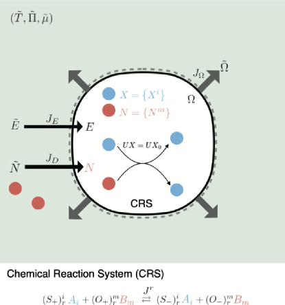
Figure 1: Diagrammatic representation of open CRSs. The chemical reactions occur with the reaction flux $J(t)=\{J^{r}(t)\}$, the $r$th reaction of which is represented as the chemical equation at the bottom. Here, $A=\{A_{i}\}$ is the label of the confined chemicals, and $B=\{B_{m}\}$ is the label of the open chemicals, which can move across the membrane with the diffusion flux $J_{D}(t)=\{J_{D}^{m}(t)\}$. In addition, $J_{E}(t)$ denotes the energy exchange rate with the environment, and $J_{\Omega}(t)$ is the volume expansion rate. Let $X=\{X^{i}\}$ and $N=\{N^{m}\}$ denote the numbers of the confined and the open chemicals in the system, respectively. Also, $\left(S_{+}\right)^{i}_{r}$ and $\left(O_{+}\right)^{m}_{r}$ denote stoichiometric coefficients of the reactants in the $r$th reaction, whereas $\left(S_{-}\right)^{i}_{r}$ and $\left(O_{-}\right)^{m}_{r}$ are the ones of the products. The stoichiometric matrices are given as $S^{i}_{r}=\left(S_{-}\right)^{i}_{r}-\left(S_{+}\right)^{i}_{r}$ and $O^{m}_{r}=\left(O_{-}\right)^{m}_{r}-\left(O_{+}\right)^{m}_{r}$. For theoretical simplicity, we ignore the tension of the membrane and assume that the membrane never bursts. The stoichiometric matrix $S=\{S^{i}_{r}\}$ has only a left kernel space. By representing the basis matrix of $\mathrm{Ker}[S^{T}]$ by $U$, $L=UX$ is conserved under the chemical reaction dynamics.

The dynamics of the number of confined chemicals $X(t)$ is described by

$$\frac{dX^{i}}{dt}=S^{i}_{r}J^{r}(t),$$ (3)

where $J(t)=\{J^{r}(t)\}$ represents the chemical reaction flux; $S=\{S^{i}_{r}\}$ denotes the stoichiometric matrix for the confined chemicals (see Fig. 1). The index $r$ runs from $r=1$ to $\mathcal{N}_{R}$, where $\mathcal{N}_{R}$ is the number of reactions. Also, Einstein’s summation convention has been employed in Eq. (3) for notational simplicity. By integrating Eq. (3), we obtain

$$X^{i}(t)=X^{i}_{0}+S^{i}_{r}\Xi^{r}(t),$$ (4)

where $X_{0}=\{X^{i}_{0}\}$ denotes the initial condition and $\Xi(t)=\{\Xi^{r}(t)\}$ is the integration of $J(t)$, i.e. the extent of reaction.

In this work, we assume that the stoichiometric matrix $S$ does not have the right kernel space,

$$\dim\mathrm{Ker}[S]=0.$$ (5)

By contrast, the left kernel space exists and generates a set of conserved quantities:

$$L=\{L^{l}=U^{l}_{i}X^{i}_{0}\}.$$ (6)

Here, $U$ is a basis matrix: $\{U_{i}^{l}\}:=(\textbf{U}^{1},\textbf{U}^{2},...)^{T}$ whose row vectors $\textbf{U}^{l}$ form the basis of $\mathrm{Ker}[S^{T}]$, i.e. $US=0$, and $l$ runs from $1$ to $\dim\mathrm{Ker}[S^{T}]$. Since we are mainly interested in the growth of the system, the time evolution of $X(t)$ should perpetually increase the number of all confined chemicals while satisfying the conservation laws (Eq. (6)). In order to realize this situation, the stoichiometric matrix $S$ should satisfy

$$\mathrm{Im}[S]\cap\mathbb{R}_{>0}^{\mathcal{N}_{X}}\neq\emptyset,$$ (7)

which is known as the condition for the productive $S$ [blokhuis2020universal]. The productive $S$ excludes the mass conservation-type laws, the existence of which trivially precludes the number of confined chemicals to increase continuously.

The number of open chemicals changes through the reactions and the diffusions. By defining the stoichiometric matrix for open chemicals as $O=\{O^{m}_{r}\}$ and the diffusion fluxes as $J_{D}(t)=\{J^{m}_{D}(t)\}$, we have

$$\frac{dN^{m}}{dt}=O^{m}_{r}J^{r}(t)+J_{D}^{m}(t).$$ (8)

Example 1: To give an illustrative example, we consider the following chemical reactions:

$$R_{1}: A_{1}+A_{3}+B_{1}\rightleftarrows 2A_{2},$$

$$R_{2}: A_{2}\rightleftarrows A_{1}+A_{3}+B_{2}.$$ (9)

Here, three confined chemicals $A=(A_{1},A_{2},A_{3})$ and two open chemicals $B=(B_{1},B_{2})$ are involved in two reactions $R_{1}$ and $R_{2}$ . The stoichiometric matrices $S$ and $O$ for the confined and open chemicals, respectively, are

(10)