Coriolis Factorizations and their Connections to Riemannian Geometry

Abstract

Many energy-based control strategies for mechanical systems require the choice of a Coriolis factorization satisfying a skew-symmetry property. This paper explores (a) if and when a control designer has flexibility in this choice, (b) what choice should be made, and (c) how to efficiently perform control computations with it. We link the choice of a Coriolis factorization to the notion of an affine connection on the configuration manifold and show how properties of the connection relate with ones of the associated factorization. Out of the choices available, the factorization based on the Christoffel symbols is linked with a torsion-free property that limits the twisting of system trajectories during passivity-based control. The machinery of Riemannian geometry also offers a natural way to induce Coriolis factorizations for constrained mechanisms from unconstrained ones, and this result provides a pathway to use the theory for efficient control computations with high-dimensional systems such as humanoids and quadruped robots.

I Introduction

If you open up a paper on the control of mechanical systems, you will often find a form of the system dynamics:

$$H(q)\dot{v}+c(q,v)+g(q)=\tau$$ (1)

where $q\in\mathcal{Q}$ represents the system configuration with $\mathcal{Q}$ the configuration manifold, $v\in\mathbb{R}^{n}$ the generalized velocities, $H(q)\in\mathbb{R}^{n\times n}$ the mass matrix, $c(q,v)\in\mathbb{R}^{n}$ the Coriolis and centripetal terms, $g(q)\in\mathbb{R}^{n}$ the generalized gravity force, and $\tau\in\mathbb{R}^{n}$ the vector of generalized applied forces. The Coriolis and centripetal terms have a quadratic dependence on the velocity variables, and thus can be factored as:

$$C(q,v)v=c(q,v)$$ (2)

where $C(q,v)\in\mathbb{R}^{n\times n}$ is referred to as a Coriolis matrix or Coriolis factorization. Overall, this paper studies the properties of Coriolis factorizations through the lens of Riemannian geometry (Fig. 1) [1], and uses this perspective to devise methods for computing factorizations with desired properties.

It is well-known that there are many ways of factoring $c(q,v)$. For example [2], if $c(q,v)=[v_{1}v_{2},0]^{\top}$, we can adopt

$$C_{a}=\scalebox{0.8}{$\begin{bmatrix}v_{2}&0\\ 0&0\end{bmatrix}$}\quad C_{b}=\scalebox{0.8}{$\begin{bmatrix}0&v_{1}\\ 0&0\end{bmatrix}$}$$

or any combination of the form $\alpha C_{a}+(1-\alpha)C_{b}$ ($\alpha\in\mathbb{R}$). Out of the many options, applications of passivity-based control often require the additional property:

$$\dot{H}=C+C^{\top}$$ (3)

which is equivalent to $\dot{H}-2C$ skew-symmetric. When working with generalized coordinates $(q^{1},\ldots,q^{n})$ with $v^{i}=\dot{q}^{i}$, a canonical choice satisfying (3) is given by:

$$C_{ij}^{\scalebox{0.5}{\scalerel*{\stackinset{c}{-.125pt}{c}{}{\scalebox{0.5}{\color[rgb]{1,1,1}{$\bigstar$}}}{$\bigstar$}}{\bigstar}}}=\Gamma_{ijk}^{\scalebox{0.5}{\scalerel*{\stackinset{c}{-.125pt}{c}{}{\scalebox{0.5}{\color[rgb]{1,1,1}{$\bigstar$}}}{$\bigstar$}}{\bigstar}}}\dot{q}^{k}$$ (4)

where Einstein summation (over $k$) convention is adopted and

$$\Gamma_{ijk}^{\scalebox{0.5}{\scalerel*{\stackinset{c}{-.125pt}{c}{}{\scalebox{0.5}{\color[rgb]{1,1,1}{$\bigstar$}}}{$\bigstar$}}{\bigstar}}}=\scalebox{1.15}{$\frac{1}{2}\left[\frac{\partial H_{ij}}{\partial q^{k}}+\frac{\partial H_{ik}}{\partial q^{j}}-\frac{\partial H_{jk}}{\partial q^{i}}\right]$}$$ (5)

are Christoffel symbols of the first kind, which play a central role in Riemannian geometry. Indeed, early work almost exclusively relied on this factorization [3, 4], with some references describing it as the unique one satisfying the skew-symmetry property [4, 5]. These observations raise fundamental questions that we undertake herein:

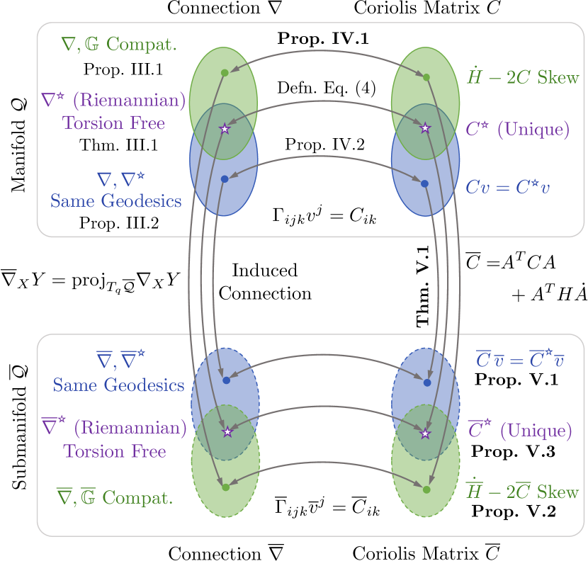
Figure 1: Roadmap. For a mechanical system on a Riemannian manifold $\mathcal{Q}$ with kinetic energy metric $\mathbb{G}$ we study how the properties of any chosen affine connection $\nabla$ relate with those of a corresponding Coriolis matrix $C$ and mass matrix $H$ w.r.t. a choice of generalized velocities $v$. We show how these properties for the system on $\mathcal{Q}$ can be related to a constrained system that evolves on a submanifold $\overline{\mathcal{Q}}$ where the dynamics are described with generalized velocities $\overline{v}$ that are related to $v$ by $v=A\overline{v}$. Bolded results indicate the main contributions of the work.

1. Given the relationship between (4) and the Christoffel symbols, is there a deeper relationship between other Coriolis factorizations and the geometry of $\mathcal{Q}$?

2. When do (2) and (3) uniquely determine $C$?

3. How does the canonical factorization (4) generalize to the case of working with generalized velocities?

4. How does one practically compute such a factorization when working with high degree-of-freedom systems?

To summarize the results of the paper, we provide short answers to these questions below, leaving a self-contained introduction of all relevant nomenclature to the main body:

1. Every factorization can be associated with an affine connection on $\mathcal{Q}$, wherein geometric properties of the connection are intimately linked with (2) and (3) (Fig. 1).

2. Factorizations satisfying (2) and (3) are uniquely defined for $n=1,2$. When $n\geq 3$, there are infinitely many such factorizations. For example, for a point mass with $\dot{p}=v\in\mathbb{R}^{3}$, Newton’s equation $f=m\dot{v}$ admits factorizations $C=\beta(p)\,(v\times)$ for any function $\beta:\mathbb{R}^{3}\rightarrow\mathbb{R}$.

3. We generalize (4) by applying a privileged connection (the Riemannian connection) to a set of (non-coordinate) basis vector fields. This connection is associated with a torsion-free [1] property that limits undesirable twisting of trajectories during passivity-based control.

4. We present new results that induce factorizations for constrained systems from unconstrained ones, and where relevant properties are inherited through the process (Fig. 1). By using the Riemannian connection for unconstrained rigid bodies, these results enable forming $C^{\scalebox{0.5}{\scalerel*{\stackinset{c}{-.125pt}{c}{}{\scalebox{0.5}{\color[rgb]{1,1,1}{$\bigstar$}}}{$\bigstar$}}{\bigstar}}}$ from (4) for general constrained mechanical systems. In the special case of an open-chain kinematic tree, the results provide broader theoretical backing to a previously presented algorithm [6, Alg. 1] for computing the Coriolis matrix. We demonstrate a generalized version of that algorithm (and one for computing the Christoffel symbols) that is applicable to systems with local closed kinematic loops in the mechanism connectivity.

The rest of the document fully develops the answers to these questions and considers their application for passivity-based control.

II Related Work

We begin by taking a step back and considering how the structure of the Coriolis terms in (1) have influenced dynamics calculation methods and the control of mechanical systems. The first numerical methods for computing the left side of (1) were Recursive Newton-Euler (RNE) approaches, appearing in the late 1970s, and motivated by dynamic analysis for walking machines [7, 8]. Developments in the early 1980s soon after applied these same methods for computed torque control [9] of robot manipulators. These and other computed torque control laws require evaluating the Coriolis terms $c(q,v)$ (so they can be exactly canceled out), which can be accomplished via RNE methods in $O(n)$ complexity.

The dependency of computed-torque controllers on accurate dynamic models for exact cancelations pushed subsequent developments of energy-based methods [10]. The original PD+ control law of Takagaki and Arimoto [11], demonstrated stability without canceling Coriolis terms, and has served as motivation for passivity-based and adaptive control from the mid-1980s to the present day [12, 3, 4, 13, 14, 15, 16]. In these contexts, a factorization is used to avoid exactly canceling Coriolis terms, and the satisfaction of the skew-symmetry property (3) for the Coriolis matrix plays a critical role in many Lyapunov arguments. Passivity-based frameworks are also central for the stability of teleoperation with time delays (e.g., the work starting with [17, 18]). Throughout these works and many robotics texts (e.g., [5, 19]), the factorization based on Christoffel symbols, originally appearing in [3], has remained almost universally adopted.

Within passivity-based control, one often requires computing the product $C(q,v)v_{r}$ where $v_{r}$ is some reference velocity. As a result, following the initial wave of theoretical advances, many authors [20, 21, 22, 23] developed variants of the RNE algorithm that were capable of computing $C(q,v)v_{r}$ in place of $C(q,v)v$ to implement passivity-based controllers efficiently. Care was taken to ensure that the recursive computations were compatible with the skew property (3), with [20] providing the first RNE method compatible with the Christoffel-consistent factorization (for systems with revolute and prismatic joints). Later, [22] provided an explicit construction for the non-uniqueness of factorizations satisfying the skew-symmetry property for general mechanisms.

While the majority of these developments were focused on manipulators, parallel advances considered Coriolis factorizations for underwater systems [24, 25], with other work pushing the theory to passivity-based control of free-floating space manipulators [26, 27]. As a common thread, these lines of work considered Coriolis factorizations for a single rigid body and related properties therein to those of a constrained system as a whole. This approach motivates our strategy taken in Sec. VI herein. Our contributions generalize these past results, showing, in hindsight, that [20] provided a skew-symmetric Newton-Euler method compatible with the Christoffel-consistent factorization for a broader class of mechanisms than originally claimed.

The transpose of a Coriolis matrix (satisfying (3)) also appears in the Hamiltonian formulation of the dynamics [28, Eq. 6] in the form $C(q,v)^{\top}v$. As a result, it can be used to implement disturbance observers based on monitoring the generalized momentum [28, 29]. This observation motivated numerical methods to compute $C$ explicitly [30, 6], the latter of which has a closely related variant that was independently developed as part of the popular C/C++ Pinocchio dynamics package [31]. In contact detection, any freedom in choosing $C$ is moot since the uniqueness of $\dot{H}v$ and $C(q,v)v$ implies that $C(q,v)^{\top}v$ will be the same for any factorization satisfying (3). An efficient method for computing this product is provided in [32] for open-chain systems. The general results herein provide computational tools to extend disturbance-observer computations to general constrained mechanisms.

More recently, passivity-based versions [33, 34, 35] of whole-body QP based-controllers (e.g., [36, 37]) have been pursued under the same robustness motivations as for original passivity-based manipulator control laws. In some cases, the configuration-space Coriolis matrix $C$ must be explicitly computed (e.g., in [34]) to construct task-space target dynamics with desired passivity properties, with the method used by [34] detailed in [38]. A common theme across these works is that passivity is treated as a “nice to have” property, in the sense that when torque or friction limits are reached, passivity can be temporarily disrupted to meet higher priority needs. The results of this paper inform the optimal choice of factorization $C$ for these works, and how to compute it most efficiently for free-floating systems that are often described using generalized speeds.

As mentioned in the introduction, the main machinery for the developments herein comes from recognizing a relationship between factorizations of the Coriolis matrix with affine connections on the configuration manifold. Given these links, the methods in the paper provide an immediate computational approach for calculating covariant derivatives [1, Chap. 2] associated with complex mechanical systems. This result could have a bearing on geometry-based optimization strategies (e.g., [39]), geometry-based observers [40], or computational workflows to assess geometric properties such as differential flatness [41] or nonlinear controllability [42]. More broadly, there is a growing interest in geometric methods for robotics [43], which suggests a potential for other impacts by linking fundamental robot modeling choices more deeply with geometric properties.

Beyond the above robot control work, the paper also builds on foundational work on geometric mechanics. In particular, our answers to Q3 are motivated by the generalization of the Christoffel symbols from [44]. The relationship noted between passivity-based control laws and affine connections in [45] and [46] also provides a starting point for one of our propositions. We make the exact connections with this past work precise throughout.

Overall, we contribute a comprehensive synthesis relating the properties of Coriolis matrices with affine connections, and detailing how these relationships can be used for computing Coriolis matrices with desired properties for complex mechanical systems described using generalized velocities.

The remainder of the document is organized as follows. In Sec. III we introduce key concepts from differential geometry through the perspective of mechanics, including an introduction to affine connections and their properties. We then establish a link between the choice of an affine connection and the choice of a Coriolis factorization in Sec. IV (answering Q1-Q3 from the intro) and demonstrate the effect of factorization choice on passivity-based control. Sec. V describes general results showing how one can induce factorizations for a system evolving on a submanifold, while Sec. VI takes the specific route of applying those results to constraining a set of rigid bodies (answering Q4), with a focus on computational considerations. Concluding remarks are given Sec. VII.

III Background

This section introduces differential geometry through the lens of mechanical systems. As such, we take a variational view on mechanics, which is then used to motivate the Riemannian geometry underlying the equations of motion. We aim to appeal to physical insight to motivate the concepts of covariant derivatives and affine connections from differential geometry. As such, the introduction of these concepts is more tutorial and less direct than defining them through a set of mathematical properties. In this regard, readers perfectly fluent in differential geometry may skip this section, though we hope they would find a few new insights along the way.

III-A Mechanical Systems

We consider a mechanical system with an $n$-dimensional configuration manifold $\mathcal{Q}$. Denoting by $\mathfrak{X}(\mathcal{Q})$ the set of smooth vector fields on $\mathcal{Q}$, we consider a collection of vector fields $X_{1},\ldots,X_{n}\in\mathfrak{X}(\mathcal{Q})$ so that at each point $q\in\mathcal{Q}$

$$\text{span}(X_{1}(q),\ldots,X_{n}(q))=T_{q}\mathcal{Q}$$

where $T_{q}\mathcal{Q}$ gives the tangent space to $\mathcal{Q}$ at $q$. We adopt generalized velocities $v\in\mathbb{R}^{n}$ to describe the dynamics of the system, such that at each $q\in Q$ we write $\dot{q}\in T_{q}\mathcal{Q}$ as $\dot{q}=X_{i}v^{i}$ with Einstein summation convention adopted. With these definitions, the potential energy $V(q)$ is purely configuration dependent, while kinetic energy can be written as $T(q,v)=\frac{1}{2}v^{\top}H(q)v$ where $H(q)\in\mathbb{R}^{n\times n}$ is the symmetric positive definite mass matrix from (1).

Via any variety of methods (e.g., Hamel’s equations, Kane’s method, Gibbs Appel, etc.), the dynamics of the system are known to take the form (1). The components of the conservative forces are given by $g_{i}(q)=\mathscr{L}_{X_{i}}{V}(q)$ where $\mathscr{L}_{X_{i}}{V}$ denotes the Lie derivative of $V$ along $X_{i}$ [murray2017mathematical, Ch. 7, Sec. 2.1].

Remark 1.

If we write our Lagrangian as $L(q,v)=\frac{1}{2}v^{\top}H(q)v-V(q)$, then the equations of motion given by Hamel’s equations [47, 48, 49] are:

$$\tau_{i}=\frac{{\rm d}}{{\rm d}t}\frac{\partial L}{\partial v^{i}}+s_{ij}^{k}\frac{\partial L}{\partial v^{k}}v^{j}-\mathscr{L}_{X_{i}}{L}$$ (6)

where $s_{ij}^{k}:\mathcal{Q}\rightarrow\mathbb{R}$ are the structure constants satisfying:

$$s^{k}_{ij}X_{k}=[X_{i},X_{j}]$$

with $[X_{i},X_{j}]$ the Lie bracket between vector fields. In the absence of nonconservative forces $\tau$, any solution $q(t)$ will be an extremal curve of the action integral

$$\textstyle{\int_{t_{0}}^{t_{f}}L(q(t),v(t)){\rm d}t}$$ (7)

under all variations with endpoints fixed.

In the common case when $X_{1},\ldots,X_{n}$ are chosen to be coordinate vector fields, generalized coordinates $q^{1},\ldots,q^{n}$ can be adopted. In this case, $[X_{i},X_{j}]=0$ pairwise (i.e., all structure constants are zero), and so (6) simplifies to the Euler-Lagrange equations. While there are many ways of defining the Coriolis matrix for the conventional Lagrangian equations, the particular choice (4) using Christoffel symbols has added benefits as discussed in the next subsection. Unfortunately, calculating the Christoffel symbols symbolically is not tractable for high-degree-of-freedom systems.

The symbols can be computed numerically for some restricted classes of mechanisms (e.g., those with prismatic and revolute joints) [6], but other systems with closed kinematic loops are not treated by available algorithms. Further, humanoid and quadruped robots are frequently modeled with a 6-DoF free joint between the world and their torso that is modeled using generalized velocities to avoid representation singularities associated with Euler angles. We aim to accommodate these general settings and do so by making use of a geometric treatment of the problem.

III-B Riemannian Geometry Through the Lens of Mechanics

The kinetic energy $T(q,v)=\frac{1}{2}v^{\top}H(q)v$ allows us to associate each point $q$ with an inner product on $T_{q}\mathcal{Q}$. We call this collection of inner products a metric, denoted $\mathbb{G}$, with the maps written as $\langle\!\langle\cdot,\cdot\rangle\!\rangle_{q}:T_{q}\mathcal{Q}\times T_{q}\mathcal{Q}\rightarrow\mathbb{R}$. We make this correspondence such that $\langle\!\langle\dot{q},\dot{q}\rangle\!\rangle_{q}=v^{\top}H(q)v$ for any $\dot{q}=X_{i}(q)v^{i}\in T_{q}\mathcal{Q}$.

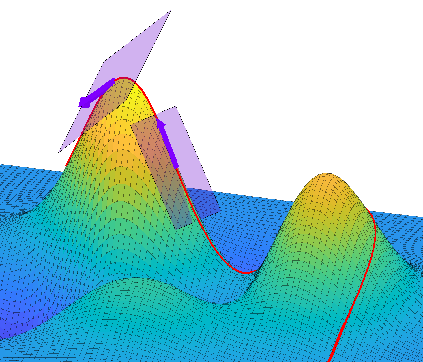
Figure 2: Motion of a particle on a frictionless surface in the absence of gravity. Equivalently, a geodesic on the surface. The particle acceleration is always normal to the surface (since constraint forces are normal to it). Equivalently, the covariant derivative of its velocity vector w.r.t. the Riemannian connection is zero along the curve.

In the absence of potential forces, the action (7) simplifies, and trajectories of the system must trace extremal curves of:

$$\textstyle{\int_{t_{0}}^{t_{f}}}\langle\!\langle\dot{q}(t),\dot{q}(t)\rangle\!\rangle_{q(t)}{\rm d}t$$

under variations with endpoints fixed. Any such trajectory also traces a path of extremal distance between its endpoints (a geodesic according to the metric). Returning to our mechanics interpretation, let us consider a point mass evolving on a frictionless 2D manifold embedded in $\mathbb{R}^{3}$ (as drawn in Fig. 2). In the absence of friction (and gravity), the motion of the point on this surface will trace a geodesic, and will evolve with a velocity of constant magnitude $\sqrt{\langle\!\langle\dot{q},\dot{q}\rangle\!\rangle}_{q}$ and an acceleration always normal to the surface. This property follows since the only forces are constraint forces, which are normal to the surface.

Put another way, for a point mass moving under the influence of constraint forces alone, the projection of the acceleration onto the local tangent is always zero. This insight motivates us to define what we call a covariant derivative for the velocity vector along the curve (a directional derivative of sorts), which is obtained by projecting the acceleration vector at each point onto the local tangent plane. For the curve to be a geodesic, this covariant derivative of the velocity must be zero along the curve.

More generally, we consider our manifold $\mathcal{Q}$ with the metric $\mathbb{G}$ (i.e., such that $(\mathcal{Q},\mathbb{G})$ defines a Riemannian manifold). We further consider $\mathcal{Q}$ isometrically embedded in some Euclidean space, where the length of any path according to the metric is simply the usual Euclidean length in the ambient space. Using a similar construction as above, we can give the rate of change of a vector field $Y$ in the direction of another $X$ as $\nabla_{X}^{\scalebox{0.5}{\scalerel*{\stackinset{c}{-.125pt}{c}{}{\scalebox{0.5}{\color[rgb]{1,1,1}{$\bigstar$}}}{$\bigstar$}}{\bigstar}}}Y$ via taking a conventional directional derivative of $Y$ in the ambient space, and projecting the result, pointwise, to the local tangent space. This manner of differentiating vectors via projection to connect nearby tangent spaces is natural, and for this reason, we call $\nabla^{\scalebox{0.5}{\scalerel*{\stackinset{c}{-.125pt}{c}{}{\scalebox{0.5}{\color[rgb]{1,1,1}{$\bigstar$}}}{$\bigstar$}}{\bigstar}}}$ the Riemannian connection associated with $(\mathcal{Q},\mathbb{G})$. For any pair of smooth vector fields $X,Y\in\mathfrak{X}(\mathcal{Q})$ and all scalar-valued functions $f$ on $\mathcal{Q}$ this operation satisfies;

1. $\nabla^{\scalebox{0.5}{\scalerel*{\stackinset{c}{-.125pt}{c}{}{\scalebox{0.5}{\color[rgb]{1,1,1}{$\bigstar$}}}{$\bigstar$}}{\bigstar}}}_{fX}Y=f\nabla^{\scalebox{0.5}{\scalerel*{\stackinset{c}{-.125pt}{c}{}{\scalebox{0.5}{\color[rgb]{1,1,1}{$\bigstar$}}}{$\bigstar$}}{\bigstar}}}_{X}Y$

2. $\nabla^{\scalebox{0.5}{\scalerel*{\stackinset{c}{-.125pt}{c}{}{\scalebox{0.5}{\color[rgb]{1,1,1}{$\bigstar$}}}{$\bigstar$}}{\bigstar}}}_{X}fY=f\nabla^{\scalebox{0.5}{\scalerel*{\stackinset{c}{-.125pt}{c}{}{\scalebox{0.5}{\color[rgb]{1,1,1}{$\bigstar$}}}{$\bigstar$}}{\bigstar}}}_{X}Y+(\mathscr{L}_{X}{f})Y$

Any bilinear mapping $\nabla:\mathfrak{X}(\mathcal{Q})\times\mathfrak{X}(\mathcal{Q})\rightarrow\mathfrak{X}(\mathcal{Q})$ (i.e., not just the Riemannian connection) satisfying the above two properties is called an affine connection, and defines an alternative manner for taking directional derivatives of a vector field. As a more restricted case, we consider any vector field $Z$ defined only along a curve $\gamma:\mathbb{R}\rightarrow\mathcal{Q}$ such that $Z(s)\in T_{\gamma(s)}\mathcal{Q}$ at each point along the curve. The covariant derivative of $Z$ along a curve $\gamma$ is denoted as $\nabla_{\dot{\gamma}}Z$ and is well defined. A curve $\gamma$ is said to be a geodesic of the connection if $\nabla_{\dot{\gamma}}\dot{\gamma}=0$. Notably, geodesics of the Riemannian connection $\nabla^{\scalebox{0.5}{\scalerel*{\stackinset{c}{-.125pt}{c}{}{\scalebox{0.5}{\color[rgb]{1,1,1}{$\bigstar$}}}{$\bigstar$}}{\bigstar}}}$ enjoy a special property in that they correspond with geodesics curves (i.e., of extremal length) for the metric $\mathbb{G}$.

An affine connection also defines a manner of parallel transporting tangent vectors along a curve. For a vector field $Z$ along a curve $\gamma$, we say that the collection of tangent vectors $Z(s)\in T_{\gamma(s)}\mathcal{Q}$ are parallel according to the connection if $\nabla_{\dot{\gamma}}Z=0$. Given some initial $Z(0)$, the condition $\nabla_{\dot{\gamma}}Z=0$ gives a differential equation for $Z(s)$ that then uniquely determines how to parallel transport $Z(0)$ along the curve. Note that parallel transport for the Riemannian connection relies on local projections to connect nearby tangent spaces. Since projections are distance optimizing, parallel transport according to $\nabla^{\scalebox{0.5}{\scalerel*{\stackinset{c}{-.125pt}{c}{}{\scalebox{0.5}{\color[rgb]{1,1,1}{$\bigstar$}}}{$\bigstar$}}{\bigstar}}}$ rules out unnecessary extra “spinning” of $Z$ around $\gamma$, and so $\nabla^{\scalebox{0.5}{\scalerel*{\stackinset{c}{-.125pt}{c}{}{\scalebox{0.5}{\color[rgb]{1,1,1}{$\bigstar$}}}{$\bigstar$}}{\bigstar}}}$ is said to be torsion-free.

It is worth mentioning that while we have introduced operations of covariant differentiation and parallel transport using an extrinsic view of a manifold $\mathcal{Q}$ (i.e., by considering an embedding of it in Euclidean space), these operations do not depend on the details of that embedding, and so can be viewed as ones defined intrinsically on the manifold itself.

Namely, we can represent $\nabla^{\scalebox{0.5}{\scalerel*{\stackinset{c}{-.125pt}{c}{}{\scalebox{0.5}{\color[rgb]{1,1,1}{$\bigstar$}}}{$\bigstar$}}{\bigstar}}}$ via a set of components at each point using our basis vector fields $X_{1},\ldots,X_{n}$. Let us consider a choice of coordinate vector fields with symbols $\Gamma_{ijk}^{\scalebox{0.5}{\scalerel*{\stackinset{c}{-.125pt}{c}{}{\scalebox{0.5}{\color[rgb]{1,1,1}{$\bigstar$}}}{$\bigstar$}}{\bigstar}}}$ defined by (5). We can relate these symbols to those of the second kind via

$$\Gamma^{i{\scalebox{0.5}{\scalerel*{\stackinset{c}{-.125pt}{c}{}{\scalebox{0.5}{\color[rgb]{1,1,1}{$\bigstar$}}}{$\bigstar$}}{\bigstar}}}}_{jk}=H^{i\ell}\Gamma_{\ell jk}^{\scalebox{0.5}{\scalerel*{\stackinset{c}{-.125pt}{c}{}{\scalebox{0.5}{\color[rgb]{1,1,1}{$\bigstar$}}}{$\bigstar$}}{\bigstar}}}$$

where $H^{ij}$ denotes $(H^{-1})_{ij}$. These symbols can be shown to give the covariant derivative of any basis vector field along another, according to:

$$\nabla_{X_{j}}^{\scalebox{0.5}{\scalerel*{\stackinset{c}{-.125pt}{c}{}{\scalebox{0.5}{\color[rgb]{1,1,1}{$\bigstar$}}}{$\bigstar$}}{\bigstar}}}X_{k}=\Gamma^{i{\scalebox{0.5}{\scalerel*{\stackinset{c}{-.125pt}{c}{}{\scalebox{0.5}{\color[rgb]{1,1,1}{$\bigstar$}}}{$\bigstar$}}{\bigstar}}}}_{jk}X_{i}$$

These relationships then uniquely specify the covariant derivative w.r.t. the Riemannian connection on any generic pair of vector fields via properties A1 and A2.

III-C Properties of Affine Connections

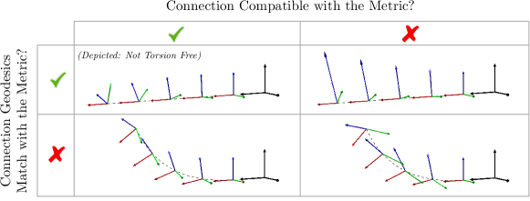
Figure 3: We consider parallel transport along the geodesics of four different affine connections. In each case, three vectors are transported – they start mutually orthogonal, and the geodesic is considered along the initial red vector. The connection is compatible with the Euclidean metric (left column) if the coordinate system remains orthonormal throughout. This notion of being compatible with the metric is distinct from the geodesics of the connection being the same as those of the Euclidean metric (top row). The upper left corner shows a connection with torsion. In this case, the unique torsion-free metric-compatible connection would instead keep the coordinate system at a constant orientation.

More generally, we can uniquely specify an affine connection $\nabla$ by fixing a definition for connection coefficients $\Gamma_{ijk}:\mathcal{Q}\rightarrow\mathbb{R}$ and defining the covariant derivative w.r.t. $\nabla$ according to $\nabla_{X_{j}}X_{k}=\Gamma^{i}_{jk}X_{i}$. Given the immense flexibility this provides, we consider a few desirable properties that we would like a connection to satisfy, and whose relationships are diagrammed in Fig. 1.

III-C1 Metric Compatibility

A connection is said to be compatible with the metric if

$$\mathscr{L}_{X}{\langle\!\langle Y,Z\rangle\!\rangle}=\langle\!\langle\nabla_{X}Y,Z\rangle\!\rangle+\langle\!\langle Y,\nabla_{X}Z\rangle\!\rangle\,.$$

which ensures that any orthonormal set of tangent vectors (rooted at the same base point) will remain orthonormal under parallel transport (See Fig. 3). Naturally, one can show that the Riemannian connection $\nabla^{\scalebox{0.5}{\scalerel*{\stackinset{c}{-.125pt}{c}{}{\scalebox{0.5}{\color[rgb]{1,1,1}{$\bigstar$}}}{$\bigstar$}}{\bigstar}}}$ is compatible with its metric $\mathbb{G}$. With this motivation, we consider the difference between the Riemannian connection and another connection according to:

$$D(X,Y,Z)=\langle\!\langle X,\nabla^{\scalebox{0.5}{\scalerel*{\stackinset{c}{-.125pt}{c}{}{\scalebox{0.5}{\color[rgb]{1,1,1}{$\bigstar$}}}{$\bigstar$}}{\bigstar}}}_{Y}Z\rangle\!\rangle-\langle\!\langle X,\nabla_{Y}Z\rangle\!\rangle$$

which we call a contorsion tensor [51], with components:

$$D_{ijk}=D(X_{i},X_{j},X_{k})=\Gamma_{ijk}^{\scalebox{0.5}{\scalerel*{\stackinset{c}{-.125pt}{c}{}{\scalebox{0.5}{\color[rgb]{1,1,1}{$\bigstar$}}}{$\bigstar$}}{\bigstar}}}-\Gamma_{ijk}$$

Proposition III.1 (Metric-Compatible Connections).

A connection $\nabla$ is compatible with a metric $\mathbb{G}$ iff its associated contorsion tensor $D$ is anti-symmetric in the first and third arguments (i.e., $D(X,Y,Z)=-D(Z,Y,X)$). Equivalently, the components $D_{ijk}$ are anti-symmetric in indices (1,3).

Proof.

See [51, Section 7.2.6] for the setup of an exercise on this result. ∎

A connection is said to be torsion-free if

$$[X,Y]=\nabla_{X}Y-\nabla_{Y}X$$

As motivated previously, this roughly ensures that vectors do not twist around a curve when parallel transported. This condition is the same as requiring that the structure constants $s^{i}_{jk}$ satisfy $s^{i}_{jk}=\Gamma^{i}_{jk}-\Gamma^{i}_{kj}$, which reduces to $\Gamma^{i}_{jk}=\Gamma^{i}_{kj}$ or equivalently $\Gamma_{ijk}=\Gamma_{ikj}$ when working with coordinate vector fields. Considerations of connections being metric-compatible and torsion-free lead to the fundamental theorem of Riemannian geometry:

Theorem III.1 (Riemannian Connection, [1]).

On a Riemannian manifold $\mathcal{Q}$ there exists a unique affine connection $\nabla$ that is compatible with the metric and torsion free. This connection is the Riemannian (or Levi-Civita) connection $\nabla^{\scalebox{0.5}{\scalerel*{\stackinset{c}{-.125pt}{c}{}{\scalebox{0.5}{\color[rgb]{1,1,1}{$\bigstar$}}}{$\bigstar$}}{\bigstar}}}$.

Remark 2.

See [52, App. 1.D] for an alternative description of metric-compatible torsion-free parallel transport.

With this result, the Riemannian connection can be uniquely specified by the so-called Koszul formula which gives that for any smooth vector fields $X,Y,Z$ [1, Thm. 3.6]

$$2\langle\!\langle X,\nabla^{\scalebox{0.5}{\scalerel*{\stackinset{c}{-.125pt}{c}{}{\scalebox{0.5}{\color[rgb]{1,1,1}{$\bigstar$}}}{$\bigstar$}}{\bigstar}}}_{Y}Z\rangle\!\rangle= \mathscr{L}_{Z}{\langle\!\langle X,Y\rangle\!\rangle}+\langle\!\langle Z,[X,Y]\rangle\!\rangle$$

$$+\mathscr{L}_{Y}{\langle\!\langle X,Z\rangle\!\rangle}+\langle\!\langle Y,[X,Z]\rangle\!\rangle$$

$$-\mathscr{L}_{X}{\langle\!\langle Y,Z\rangle\!\rangle}+\langle\!\langle X,[Y,Z]\rangle\!\rangle$$

This definition then allows us to consider generalized Christoffel symbols when working with non-coordinate basis vector fields, which are given according to:

$$\scaleobj{.97}{2\Gamma_{ijk}^{\scalebox{0.5}{\scalerel*{\stackinset{c}{-.125pt}{c}{}{\scalebox{0.5}{\color[rgb]{1,1,1}{$\bigstar$}}}{$\bigstar$}}{\bigstar}}}} \scaleobj{.97}{=2\langle\!\langle X_{i},\nabla_{X_{j}}X_{k}\rangle\!\rangle}$$ (8)

$$\scaleobj{.97}{=\mathscr{L}_{X_{k}}{H_{ij}}+\mathscr{L}_{X_{j}}{H_{ik}}-\mathscr{L}_{X_{i}}{H_{jk}}}$$

$$\scaleobj{.97}{~{}~{}+\langle\!\langle X_{k},[X_{i},X_{j}]\rangle\!\rangle+\langle\!\langle X_{j},[X_{i},X_{k}]\rangle\!\rangle+\langle\!\langle X_{i},[X_{j},X_{k}]\rangle\!\rangle}$$

$$\scaleobj{.97}{=\mathscr{L}_{X_{k}}{H_{ij}}+\mathscr{L}_{X_{j}}{H_{ik}}-\mathscr{L}_{X_{i}}{H_{jk}}+s_{kij}+s_{jik}+s_{ijk}}$$

where $s_{ijk}=H_{i\ell}s^{\ell}_{jk}$. If you removed the last term $s_{ijk}$ on the last line of (8), the definition would be symmetric in its (2,3) indices. So, letting $\Gamma^{\scalebox{0.5}{\scalerel*{\stackinset{c}{-.125pt}{c}{}{\scalebox{0.5}{\color[rgb]{1,1,1}{$\bigstar$}}}{$\bigstar$}}{\bigstar}}}_{i(jk)}=\frac{1}{2}(\Gamma^{\scalebox{0.5}{\scalerel*{\stackinset{c}{-.125pt}{c}{}{\scalebox{0.5}{\color[rgb]{1,1,1}{$\bigstar$}}}{$\bigstar$}}{\bigstar}}}_{ijk}+\Gamma^{\scalebox{0.5}{\scalerel*{\stackinset{c}{-.125pt}{c}{}{\scalebox{0.5}{\color[rgb]{1,1,1}{$\bigstar$}}}{$\bigstar$}}{\bigstar}}}_{ikj})$ denote the symmetrized version, we have

$$\Gamma^{\scalebox{0.5}{\scalerel*{\stackinset{c}{-.125pt}{c}{}{\scalebox{0.5}{\color[rgb]{1,1,1}{$\bigstar$}}}{$\bigstar$}}{\bigstar}}}_{ijk}=\Gamma^{\scalebox{0.5}{\scalerel*{\stackinset{c}{-.125pt}{c}{}{\scalebox{0.5}{\color[rgb]{1,1,1}{$\bigstar$}}}{$\bigstar$}}{\bigstar}}}_{i(jk)}+\frac{1}{2}s_{ijk}$$ (9)

We’ll see the significance of this result in Sec. VI-D.

III-C2 Geodesic Agreement

We note that this characterization of a connection being “compatible with the metric” is different from requiring the geodesics of the connection to match those of the metric. We further build on this distinction through the following results.

Proposition III.2 (Geodesic Agreement).

A connection gives the same geodesics as the Riemannian connection iff its contorsion tensor is anti-symmetric in its second and third arguments (i.e., $D(X,Y,Z)=-D(X,Z,Y)$. Equivalently, the components $D_{ijk}$ are anti-symmetric in indices (2,3).

Out of all possible connections with Riemannian geodesics, the Riemannian one turns out the only one that is torsion-free.

Theorem III.2.

Given any affine connection on $\mathcal{Q}$, there is a unique torsion-free connection with the same geodesics.

Proof.

See [53, Chapter 6, Corollary 17]. ∎

If we combine Prop. III.1 and Thm. III.2, we see that we still have a great deal of freedom even when restricting to connections that a) are compatible with the metric and b) give the same geodesics as the metric.

Corollary III.1.

A connection is metric-compatible and gives the same geodesics as the Riemannian connection iff its contorsion tensor $D(X,Y,Z)$ is totally anti-symmetric (i.e., in any pair of arguments). Equivalently, the components $D_{ijk}$ are anti-symmetric in any pair of indices.

Corollary III.2.

For manifolds of dimension one or two, there is a unique connection (namely the Riemannian connection) that is metric-compatible and gives the same geodesics as the Riemannian connection. In dimensions three or higher, there are an infinity of such connections.

Proof.

Consider any $n$-dimensional vector space $V$. The vector space of totally antisymmetric rank $d$ tensors on $V$ has dimension $\begin{pmatrix}n\\ d\end{pmatrix}=\frac{n!}{d!(n-d)!}$. Since the contorsion tensor over $\mathcal{Q}$ is rank 3, at each point $q\in\mathcal{Q}$, the vector space of anti-symmetric tensors on $T_{q}\mathcal{Q}$ will have dimensionality $\begin{pmatrix}n\\ 3\end{pmatrix}$. Thus, in dimensions $n=1,2$ the contortion tensor must be zero. When $n=3$, the set of anti-symmetric contortion tensor fields will be isomorphic to the set of scalar fields $\mathcal{Q}$, presenting an infinity of options. Beyond $n=3$, there is only additional freedom. ∎

Remark 3.

The total anti-symmetry of the contorsion tensor $D(X,Y,Z)$ equivalently implies that it represents a 3-form (i.e., a volume form).

Referring back to Fig. 1, we see that the upper-left of the diagram displays a large area of overlap between those connections that are metric compatible and those whose geodesics are Riemannian, with the Riemannian connection residing in this intersection.

IV Relationship between Coriolis Factorizations and Affine Connections

This section creates a bridge between the properties of an affine connection and those of a Coriolis factorization that we derive from it. We first note that when working with coordinate vector fields, the Christoffel symbols are symmetric in the (2,3) indices, which means that we have the equivalence $C_{ij}^{\scalebox{0.5}{\scalerel*{\stackinset{c}{-.125pt}{c}{}{\scalebox{0.5}{\color[rgb]{1,1,1}{$\bigstar$}}}{$\bigstar$}}{\bigstar}}}=\Gamma_{ijk}^{\scalebox{0.5}{\scalerel*{\stackinset{c}{-.125pt}{c}{}{\scalebox{0.5}{\color[rgb]{1,1,1}{$\bigstar$}}}{$\bigstar$}}{\bigstar}}}v^{k}=\Gamma_{ikj}^{\scalebox{0.5}{\scalerel*{\stackinset{c}{-.125pt}{c}{}{\scalebox{0.5}{\color[rgb]{1,1,1}{$\bigstar$}}}{$\bigstar$}}{\bigstar}}}v^{k}$. When working with generalized velocities, we lose the $(2,3)$ symmetry of the symbols, and instead need to choose: Do we define our Coriolis matrix associated with the Riemannian connection via $C_{ij}^{\scalebox{0.5}{\scalerel*{\stackinset{c}{-.125pt}{c}{}{\scalebox{0.5}{\color[rgb]{1,1,1}{$\bigstar$}}}{$\bigstar$}}{\bigstar}}}=\Gamma^{\scalebox{0.5}{\scalerel*{\stackinset{c}{-.125pt}{c}{}{\scalebox{0.5}{\color[rgb]{1,1,1}{$\bigstar$}}}{$\bigstar$}}{\bigstar}}}_{ijk}v^{k}$, $\Gamma^{\scalebox{0.5}{\scalerel*{\stackinset{c}{-.125pt}{c}{}{\scalebox{0.5}{\color[rgb]{1,1,1}{$\bigstar$}}}{$\bigstar$}}{\bigstar}}}_{ikj}v^{k}$, or the symmetric part of the symbols $\Gamma^{\scalebox{0.5}{\scalerel*{\stackinset{c}{-.125pt}{c}{}{\scalebox{0.5}{\color[rgb]{1,1,1}{$\bigstar$}}}{$\bigstar$}}{\bigstar}}}_{i(jk)}v^{j}$? We find that, for general connections, the fruitful pairing is to choose:

$$C_{ik}(q,v)=\Gamma_{ijk}(q)\,v^{j}$$ (10)

in the sense that this definition allows us to directly relate properties of a Coriolis matrix with those of a connection.

Our first result concerns passivity and metric compatibility.

Proposition IV.1 (Skew-symmetry and Metric Compatibility).

Consider a Coriolis matrix definition $C(q,v)$ and a connection $\nabla$ related via (10). The connection is compatible with the metric iff $\dot{H}-2C$ is skew-symmetric pointwise.

Proof.

We consider the forward implication via computation:

$$\phantom{=}\dot{H}_{ij}-C_{ij}-C_{ji}$$ (11)

$$=\mathscr{L}_{X_{k}}{\langle\!\langle X_{i},X_{j}\rangle\!\rangle}\,v^{k}-\langle\!\langle X_{i},\nabla_{X_{k}}X_{j}\rangle\!\rangle v^{k}-\langle\!\langle X_{j},\nabla_{X_{k}}X_{i}\rangle\!\rangle v^{k}$$

$$=\left(\langle\!\langle\nabla_{X_{k}}X_{i},X_{j}\rangle\!\rangle+\langle\!\langle X_{i},\nabla_{X_{k}}X_{j}\rangle\!\rangle\right)v^{k}$$

$$~{}~{}~{}~{}~{}~{}-\left(\langle\!\langle X_{i},\nabla_{X_{k}}X_{j}\rangle\!\rangle+\langle\!\langle X_{j},\nabla_{X_{k}}X_{i}\rangle\!\rangle\right)v^{k}=0$$

where we have used the metric compatibility when going from the second to the third line.

For the reverse direction, the second line of (11) is assumed zero, which gives that $\mathscr{L}_{X_{i}}{\langle\!\langle}X_{j},X_{k}\rangle\!\rangle=\langle\!\langle\nabla_{X_{i}}X_{j},X_{k}\rangle\!\rangle+\langle\!\langle X_{j},\nabla_{X_{i}}X_{k}\rangle\!\rangle$. To show metric compatibility, we must show that the same type of property holds on arbitrary vector fields. We consider the triple of vector fields $X,Y,Z\in\mathfrak{X}(\mathcal{Q})$ expressed as $X=X_{i}x^{i}$, $Y=X_{i}y^{i}$, $Z=X_{i}z^{i}$. Via using properties of the Lie derivative, we have

$$\scaleobj{.96}{\mathscr{L}_{X}{\langle\!\langle Y,Z\rangle\!\rangle}} \scaleobj{.96}{=\mathscr{L}_{X_{i}x^{i}}{\langle\!\langle X_{j}y^{j},X_{k}z^{k}\rangle\!\rangle}}$$

$$\scaleobj{.96}{=x^{i}(\mathscr{L}_{X_{i}}{y^{j}z^{k}})\langle\!\langle X_{j},X_{k}\rangle\!\rangle+x^{i}y^{j}z^{k}\mathscr{L}_{X_{i}}{\langle\!\langle X_{j},X_{k}\rangle\!\rangle}}$$

We use the second line of (11) to carry out the Lie derivative $\mathscr{L}_{X_{i}}{\langle\!\langle}X_{j},X_{k}\rangle\!\rangle$, which leads to:

$$\nabla_{X}\langle\!\langle Y,Z\rangle\!\rangle =x^{i}z^{k}\langle\!\langle\nabla_{X_{i}}X_{j}y^{j},X_{k}\rangle\!\rangle+x^{i}y^{j}\langle\!\langle X_{j},\nabla_{X_{i}}X_{k}z^{k}\rangle\!\rangle$$

$$=\langle\!\langle\nabla_{X}Y,Z\rangle\!\rangle+\langle\!\langle Y,\nabla_{X}Z\rangle\!\rangle$$

This proves the reverse implication. ∎

Remark 4.

The forward implication was discussed in [45, pg. 94] when working with coordinate basis vector fields.

Our second result considers whether the definition of the Coriolis matrix gives the correct equations of motion:

Proposition IV.2.

Consider a Coriolis matrix definition $C(q,v)$ and a connection $\nabla$ related by (10). The connection gives the same geodesics as the Riemannian connection iff the Coriolis matrix satisfies $Cv=C^{\scalebox{0.5}{\scalerel*{\stackinset{c}{-.125pt}{c}{}{\scalebox{0.5}{\color[rgb]{1,1,1}{$\bigstar$}}}{$\bigstar$}}{\bigstar}}}v$, where $C^{\scalebox{0.5}{\scalerel*{\stackinset{c}{-.125pt}{c}{}{\scalebox{0.5}{\color[rgb]{1,1,1}{$\bigstar$}}}{$\bigstar$}}{\bigstar}}}$ is the factorization corresponding to the Riemannian connection.

Corollary IV.1.

Any Coriolis factorization that satisfies the skew-symmetry property and gives the correct dynamics is derived from a connection whose coefficients differ from the Riemannian connection by a totally anti-symmetric contorsion tensor. There is a unique such factorization in dimensions $n=1$ and $n=2$, but an infinite number of admissible factorizations in dimensions $n=3$ and higher.

Proof.

The result follows from combining Corollary III.2 with Propositions IV.1 and IV.2. ∎

The previous corollary gives us a way to construct all possible factorizations satisfying the skew-symmetry property (3) and providing the correct dynamics. In dimension $n=3$, given one such factorization $C_{\rm old}(q,v)$, we can construct another according to:

$$C_{\rm new}(q,v)=C_{\rm old}(q,v)+\beta(q)(v\times)$$

where $\beta:\mathcal{Q}\rightarrow\mathbb{R}$. More generally, when $n>3$ we can consider defining a selector matrix

$$S_{ijk}=\begin{bmatrix}e_{i}&e_{j}&e_{k}\end{bmatrix}^{\top}\,,$$

where $e_{i},e_{j},e_{k}\in\mathbb{R}^{n}$ are the $i$-th, $j$-th, and $k$-th coordinate unit vectors, resepectively. We can then generalize the above construction according to:

$$C_{\rm new}(q,v)=C_{\rm old}(q,v)+\sum_{i<j<k}\beta_{ijk}(q)S_{ijk}^{\top}(S_{ijk}v\times)S_{ijk}$$ (12)

where each $\beta_{ijk}:\mathcal{Q}\rightarrow\mathbb{R}$ can be chosen independently.

IV-A Interpretation in Passivity-Based Control

IV-A1 Setup

In this subsection, we consider the use case of these Coriolis matrices in passivity-based control, and explore the role that the torsion-free property has on the resulting trajectories. To do so, we employ the tracking control component of [3]. For simplicity, we consider the case where we are working with generalized coordinates. Given a desired trajectory $q_{d}(t)$, we consider a time-varying vector field $\dot{q}_{r}(q,t)=\dot{q}_{d}(t)+\Lambda(q-q_{d}(t))$ where $\Lambda>0$ is a gain matrix that is used to control convergence speed.

Following [3], we form the sliding variable:

$$s=\dot{q}-\dot{q}_{r}$$

where the task of tracking the desired trajectory $q_{d}(t)$ can now be achieved via regulating $s\rightarrow 0$.

This definition leads to a certainty-equivalence control law

$$\tau=\hat{H}(q)\ddot{q}_{r}+\hat{C}(q,\dot{q})\dot{q}_{r}+\hat{g}(q)-K_{D}s$$ (13)

where $\hat{H}$, $\hat{C}$, and $\hat{g}$ represent estimates of the mass matrix, Coriolis matrix, and gravity terms, and $K_{D}\succ 0$ is a user-chosen gain matrix. We consider estimates for the classical inertial parameters of the mechanism [54] as $\hat{\pi}$, which allows expressing the control law (13) above as:

$$\tau=Y(q,\dot{q},\dot{q}_{r},\ddot{q}_{r})\hat{\pi}-K_{D}s$$

where $Y(q,\dot{q},\dot{q}_{r},\ddot{q}_{r})$ is often referred to as the Slotine-Li regressor matrix [55, 38].

Considering the closed-loop behavior under this control law, the sliding variable then evolves as [3]

$$H(q)\dot{s}+(C(q,\dot{q})+K_{D})s=Y(q,\dot{q},\dot{q}_{r},\ddot{q}_{r})\tilde{\pi}$$

where $\tilde{\pi}=\hat{\pi}-\pi$ gives the parameter error. To study the regulation of $s\rightarrow 0$, we consider the Lyapunov candidate

$$V=\frac{1}{2}s^{\top}H(q)s$$

which, using any factorization satisfying $\dot{H}=C+C^{\top}$, can be shown to have rate of change:

$$\dot{V}=-s^{\top}K_{D}s+s^{\top}Y\tilde{\pi}$$ (14)

When the parameter error $\tilde{\pi}=0$, we have convergence to $s\rightarrow 0$, while when $\tilde{\pi}$ is non-zero, we can adapt the estimate [3]. For the purposes of the following example, we leave a persistent parameter error to see how the controller performs with modeling inaccuracy.

Remark 5.

While we viewed $s,\dot{q}_{r}\in\mathbb{R}^{n}$ in this example, if we instead view $\dot{q}_{r}$ as a time-varying vector field over $\mathcal{Q}$ with $s(t)=\dot{q}(t)-\dot{q}_{r}(q(t),t)\in T_{q(t)}\mathcal{Q}$, then, along any trajectory

$$H(q)\dot{s}+C(q,\dot{q})s=H(q)\nabla_{\dot{q}}s$$

so that the closed-loop dynamics then provide:

$$H(q)\nabla_{\dot{q}}s+K_{D}s=Y(q,\dot{q},\dot{q}_{r},\ddot{q}_{r})\tilde{\pi}$$

Remark 6.

The above construction created the reference velocity field $\dot{q}_{r}(q,t)$ to provide convergence to $q_{d}(t)$. However, one can consider generating this reference velocity field in many other manners. For example, it could be constructed to provide convergence to a submanifold, convergence in task-space [21, 56], or to a desired limit cycle, with $\ddot{q}_{r}\in\mathbb{R}^{n}$ then defined based on the time differentiation of coordinates of this vector field along the trajectory.

Alternatively, as discussed in [57, Example 3.4] the reference dynamics can be specified at the acceleration level via defining desired accelerations $\ddot{q}_{d}(t,q,\dot{q})$ directly and then constructing $\dot{q}_{r}$ via integrating the dynamics:

$$\ddot{q}_{r}(t)=-k(\dot{q}_{r}(t)-\dot{q}(t))+\ddot{q}_{d}(t,q,\dot{q})\,.$$

In that case, the classical analysis holds so that $s\rightarrow 0$.

IV-A2 Example

As motivated in the introduction, we consider the simple example of tracking a trajectory for a point mass in 3D. We estimate the point mass as $\hat{m}=0.9$ kg with the true mass $m=1$ kg. The tracking task is chosen as following a line with varying velocity such that $q_{d}(t)=[t+\sin(t),~{}0,~{}0]^{\top}$.

In the first case, we use the Coriolis matrix $C=0$ which corresponds to the torsion-free connection, and we use parameters $\Lambda=1$ and $K_{D}=1$. The resulting trajectories are shown vs. time in Fig. 4. The results are uneventful, and the trajectory converges to near-zero error. The error does not exactly approach zero, even for a longer simulation, since there is a model mismatch.

As a second case, we consider the Coriolis factorization $C=-5(v\times)$. This factorization feels a bit unreasonable since the Coriolis terms are zero in this case. However, since $H(q)=m\mathbf{1}_{3}$ where $\mathbf{1}_{3}$ the identity matrix, we have $\dot{H}=0$, and so any skew-symmetric $C$ will satisfy the skew property (3). Using any scalar multiple of the Cartesian cross-product matrix $(v\times)$ (or more generally any scalar configuration-dependent function times the cross-product matrix) therefore satisfies (2) and (3). The resulting trajectory is plotted vs. time in Fig. 5. The trajectory has higher frequency content than the previous case and thus would be comparatively undesirable for deployment on a physical system. Note that the frequency content can be driven even higher by selecting a more extreme factorization (e.g., $-10(v\times)$) away from $C^{\scalebox{0.5}{\scalerel*{\stackinset{c}{-.125pt}{c}{}{\scalebox{0.5}{\color[rgb]{1,1,1}{$\bigstar$}}}{$\bigstar$}}{\bigstar}}}$.

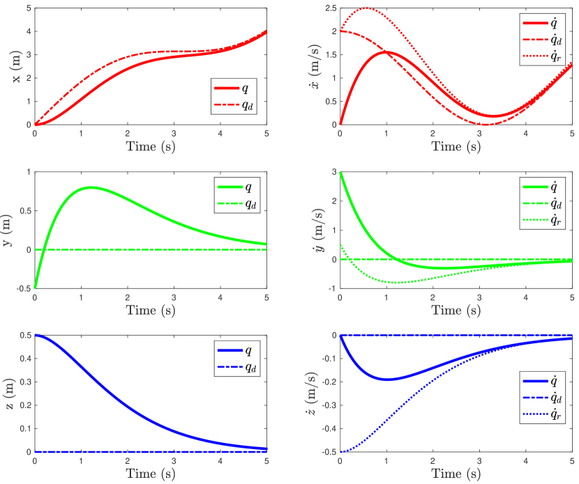
Figure 4: Point mass state trajectories, torsion-free.

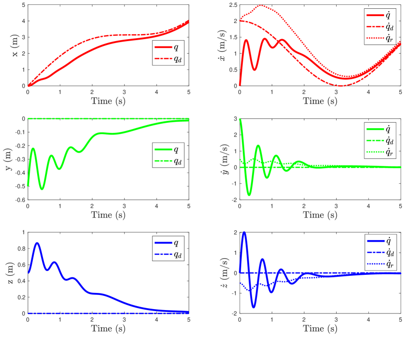
Figure 5: Point mass state trajectories, non-torsion-free.

The effects of torsion are better demonstrated in Fig. 6, which shows parametric trajectory in 3D space. The point mass starts nearest (at $x=0$) and moves away (up and to the right in the figure) as time progresses. At the beginning of the trajectory, the mass has a velocity to the left, while the reference velocity is moving forward. The terms from the Coriolis factorization $-5(v\times)v_{r}$ cause a counterproductive upward acceleration that sends the mass further from the target.

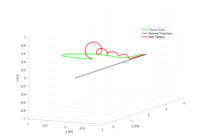
Figure 6: Point mass trajectories, torsion free vs. with torsion.

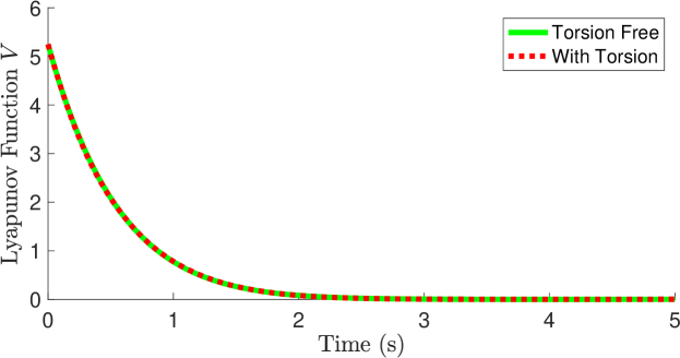
Figure 7: Lyapunov function evolution for point-mass example: torsion-free vs. with torsion.

This difference in behavior between the two cases is masked by conventional Lyapunov analysis, as (14) is independent of the choice of $C$. Fig. 7 shows the Lyapunov function evolution for both setups, and in this case, the evolution is nearly identical (the evolution is not exactly identical, which becomes more apparent for larger mismatch in the mass estimate). While this finding may be surprising, it is worth noting that a Lyapunov function value provides a condensed scalar indicator of progress, and, as such, trajectories can “spin” around level sets of $V$ without changing its value. With this in mind, there is quite a great deal of freedom in how the state trajectory from a controller may evolve, even for the exact same graph of $V$ over time.

These numerical experiments show the empirical effects of deviating from the Christoffel-consistent Coriolis matrix. Our subsequent section provides the tools that will allow us to construct it for practical systems of interest.

V Changes/Reduction of Coordinates

This section considers how the definition of the Coriolis matrix can be transformed under a change of basis vector fields, or when the system dynamics are restricted to a submanifold. The motivation for this latter case is based on the fact that generic mechanical systems can be considered as a collection of rigid bodies. For a single rigid body, it is well-understood how one can construct the Riemannian connection [58] or other metric-compatible connections. Thus, from a computational point of view, it would be desirable to understand how we may derive a connection for a complex multi-body system from the connections for the bodies themselves, and to understand the properties of connections that result from such operations. Again, the opening Fig. 1 diagrams the main results as a roadmap for what follows.

V-A Induced Metric and Connection

Consider a submanifold $\overline{\mathcal{Q}}\subseteq\mathcal{Q}$ with generalized speeds $\overline{v}\in\mathbb{R}^{m}$ along some frame vector fields $\overline{X}_{1},\ldots,\overline{X}_{m}\in\mathfrak{X}(\overline{\mathcal{Q}})$. At each $q\in\overline{\mathcal{Q}}$ we can write $\overline{X}_{j}(q)=A^{i}_{j}(q)X_{i}(q)$ for some coefficients $A^{i}_{j}(q)$ and arrange these coefficients into a matrix $A(q)\in\mathbb{R}^{n\times m}$ such that $A^{i}_{j}$ denotes the $i$-th row and $j$-column of the matrix $A$. We note that since for any tangent vector in $T_{q}\overline{\mathcal{Q}}$ we can write $X_{i}v^{i}=\overline{X}_{j}\overline{v}^{j}$, we also have:

$$\overline{X}_{j}\overline{v}^{j}=(A^{i}_{j}X_{i})\overline{v}^{j}=X_{i}v^{i}$$

and so it follows that $v^{i}=A^{i}_{j}\overline{v}^{j}$, i.e.,

$$v=A\overline{v}$$ (15)

With these definitions, the representation of the induced metric $\overline{\mathbb{G}}$ on $\overline{\mathcal{Q}}$ [44] is given by a new mass matrix $\overline{H}$ with entries:

$$\overline{H}_{ij}=\langle\!\langle\overline{X}_{i},\overline{X}_{j}\rangle\!\rangle=A^{k}_{i}H_{k\ell}A^{\ell}_{j}$$

and, as a result: $\overline{H}=A^{\top}HA$.

A question then regards how we might be able to achieve something similar for inducing Coriolis factorizations. To do so, we consider inducing a connection on $\overline{\mathcal{Q}}$ from one on $\mathcal{Q}$ in the following manner. Let us take a curve on $\overline{\mathcal{Q}}$ and a vector field along it, and view both as associated with $\mathcal{Q}$. We can then use the connection on $\mathcal{Q}$ to take our covariant derivative, and project the result back to the local tangent for $\overline{\mathcal{Q}}$. In other words, for any $X,Y\in\mathfrak{X}(\overline{\mathcal{Q}})$ we define our induced connection $\overline{\nabla}$ so that at any $q\in\overline{\mathcal{Q}}$:

$$\overline{\nabla}_{X}Y(q)={\rm proj}_{T_{q}\overline{\mathcal{Q}}}\nabla_{X}Y(q)$$

where the projection of any vector $W\in T_{q}\mathcal{Q}$ is given by:

$${\rm proj}_{T_{q}\overline{\mathcal{Q}}}W=\operatorname*{argmin}_{Z}\langle\!\langle Z-W,Z-W\rangle\!\rangle_{q}$$

Given our extrinsic construction for the Riemannian connection, it follows that inducing a connection $\overline{\nabla}$ on $\overline{\mathcal{Q}}$ from the Riemannian connection $\nabla^{\scalebox{0.5}{\scalerel*{\stackinset{c}{-.125pt}{c}{}{\scalebox{0.5}{\color[rgb]{1,1,1}{$\bigstar$}}}{$\bigstar$}}{\bigstar}}}$ on $\mathcal{Q}$ gives the Riemannian connection on $\overline{\mathcal{Q}}$, i.e., that

$$\overline{\nabla}_{X}^{\scalebox{0.5}{\scalerel*{\stackinset{c}{-.125pt}{c}{}{\scalebox{0.5}{\color[rgb]{1,1,1}{$\bigstar$}}}{$\bigstar$}}{\bigstar}}}Y(q)={\rm proj}_{T_{q}\overline{\mathcal{Q}}}\nabla_{X}^{\scalebox{0.5}{\scalerel*{\stackinset{c}{-.125pt}{c}{}{\scalebox{0.5}{\color[rgb]{1,1,1}{$\bigstar$}}}{$\bigstar$}}{\bigstar}}}Y(q)$$ (16)

V-B Coriolis Factorizations for Constrained Systems

We now consider $\overline{\mathcal{Q}}$ to be the configuration space of a constrained mechanism, with $\mathcal{Q}$ the configuration manifold when constraints are freed.

Theorem V.1.

Consider any connection $\nabla$ on $\mathcal{Q}$ with associated Coriolis matrix $C$. The Coriolis matrix associated with the induced connection on $\overline{\mathcal{Q}}$ is given by

$$\overline{C}=A^{\top}CA+A^{\top}H\dot{A}$$ (17)

where $\dot{A}_{j}^{i}=\mathscr{L}_{\overline{X}_{k}}{A^{i}_{j}}\overline{v}^{k}$

Proof.

We first note that the projection for the induced connection means that the difference $\nabla_{\overline{X}_{j}}\overline{X}_{k}-\overline{\nabla}_{\overline{X}_{j}}\overline{X}_{k}$ will be orthogonal to $T_{q}\overline{\mathcal{Q}}$. As such, for any $i=1,\dots,m$:

$$\langle\!\langle\overline{X}_{i},\nabla_{\overline{X}_{j}}\overline{X}_{k}-\overline{\nabla}_{\overline{X}_{j}}\overline{X}_{k}\rangle\!\rangle=0.$$

This means that the coefficients for the corresponding induced connection on $\overline{\mathcal{Q}}$ are given by $\overline{\Gamma}{}_{ijk}=\langle\!\langle\overline{X}_{i},\nabla_{\overline{X}_{j}}\overline{X}_{k}\rangle\!\rangle$. As a result, we have $\overline{C}_{ij}=\langle\!\langle\overline{X}_{i},\nabla_{\overline{X}_{k}}\overline{X}_{j}\rangle\!\rangle\overline{v}^{k}=\langle\!\langle\overline{X}_{i},\nabla_{\dot{q}}\overline{X}_{j}\rangle\!\rangle$ as a starting point. Proceeding with computations:

$$\overline{C}_{ij} =\langle\!\langle\overline{X}_{i},\nabla_{\dot{q}}\overline{X}_{j}\rangle\!\rangle$$

$$=\langle\!\langle A_{i}^{k}X_{k},\nabla_{\dot{q}}A_{j}^{\ell}X_{\ell}\rangle\!\rangle$$

$$=\langle\!\langle A_{i}^{k}X_{k},\dot{A}_{j}^{\ell}X_{\ell}+A_{j}^{\ell}\nabla_{\dot{q}}X_{\ell}\rangle\!\rangle$$

$$=\langle\!\langle A_{i}^{k}X_{k},\dot{A}_{j}^{\ell}X_{\ell}+A_{j}^{\ell}\nabla_{X_{w}}X_{\ell}\,v^{w}\rangle\!\rangle$$

$$=A_{i}^{k}H_{k\ell}\dot{A}_{j}^{\ell}+A_{i}^{k}\Gamma_{kw\ell}v^{w}A^{\ell}_{j}$$

$$=A_{i}^{k}H_{k\ell}\dot{A}_{j}^{\ell}+A_{i}^{k}C_{k\ell}A^{\ell}_{j}$$

which implies that $\ \overline{C}=A^{\top}CA+A^{\top}H\dot{A}$. ∎

As the main theoretical results of the paper, we show that the passivity, geodesic, and Riemannian connection properties of the Coriolis matrix on $\mathcal{Q}$ are inherited by the Coriolis matrix definition on $\overline{\mathcal{Q}}$ via the transformation law (17).

Proposition V.1.

Consider a choice of generalized velocities on $\mathcal{Q}$ and another on $\overline{\mathcal{Q}}\subseteq\mathcal{Q}$ related by (15). Under the transformation law (17), if $C$ satisfies skew-symmetry property (3) for $\mathcal{Q}$ then $\overline{C}$ does for $\overline{\mathcal{Q}}$.

Proof.

By computation.

$$\dot{\overline{H}}-\overline{C}-\overline{C}\,{}^{\top} =\dot{A}^{\top}HA+A^{\top}\dot{H}A+A^{\top}H\dot{A}$$

$$~{}~{}~{}-A^{\top}CA-A^{\top}H\dot{A}-A^{\top}C^{\top}A+\dot{A}^{\top}HA$$

$$=A^{\top}(\dot{H}-C-C^{\top})A=0$$

∎

Proposition V.2.

Consider a choice of generalized velocities on $\mathcal{Q}$ and another on $\overline{\mathcal{Q}}\subseteq\mathcal{Q}$ related by (15). Under the transformation law (17) if $C$ gives the correct dynamics on $\mathcal{Q}$, then $\overline{C}$ does on $\overline{\mathcal{Q}}$.

Proof.

By computation. We use the property that the Coriolis matrix $C^{\scalebox{0.5}{\scalerel*{\stackinset{c}{-.125pt}{c}{}{\scalebox{0.5}{\color[rgb]{1,1,1}{$\bigstar$}}}{$\bigstar$}}{\bigstar}}}$ associated with the Riemannian connection gives the correct dynamics.

$$\overline{C}\,\overline{v} =(A^{\top}CA+A^{\top}H\dot{A})\overline{v}=(A^{\top}C^{\scalebox{0.5}{\scalerel*{\stackinset{c}{-.125pt}{c}{}{\scalebox{0.5}{\color[rgb]{1,1,1}{$\bigstar$}}}{$\bigstar$}}{\bigstar}}}A+A^{\top}H\dot{A})\overline{v}=\overline{C}^{\scalebox{0.5}{\scalerel*{\stackinset{c}{-.125pt}{c}{}{\scalebox{0.5}{\color[rgb]{1,1,1}{$\bigstar$}}}{$\bigstar$}}{\bigstar}}}\,\overline{v}$$

∎

Proposition V.3.

Consider a choice of generalized velocities on $\mathcal{Q}$ and another on $\overline{\mathcal{Q}}\subseteq\mathcal{Q}$ related by (15). Under the transformation law (17), if $C=C^{\scalebox{0.5}{\scalerel*{\stackinset{c}{-.125pt}{c}{}{\scalebox{0.5}{\color[rgb]{1,1,1}{$\bigstar$}}}{$\bigstar$}}{\bigstar}}}$ for $\mathcal{Q}$ then $\overline{C}=\overline{C}\,{}^{\scalebox{0.5}{\scalerel*{\stackinset{c}{-.125pt}{c}{}{\scalebox{0.5}{\color[rgb]{1,1,1}{$\bigstar$}}}{$\bigstar$}}{\bigstar}}}$ for $\overline{\mathcal{Q}}$.

Proof.

The result follows from (16) and Thm. V.1. ∎

Remark 7.

A special case of Prop. V.3 was proved in [6, Thm. 1] when considering a change of generalized coordinates.

Remark 8.

It is interesting to note that, within passivity-based task-space control [34], the task-space Coriolis matrix can be constructed from a transformation law with the same structural form as (17). Given a task-space Jacobian $J$, one can construct $A=H^{-1}J^{\top}\varLambda$ where $\varLambda=(JH^{-1}J^{\top})^{-1}$ is the task-space inertia matrix. Then, the task-space inertia matrix is equivalently given by $\varLambda=A^{\top}HA$, while the Coriolis matrix given by $C_{\rm task}=A^{\top}CA+A^{\top}H\dot{A}$ matches (with some algebra) the one given in [34, Eq. 11]. Therein, it is shown that if $\dot{H}-2C$ is skew-symmetric, then $\dot{\varLambda}-2C_{\rm task}$ is skew-symmetric as well. This observation suggests properties of the transformation equation in (17) that may extend beyond induced connections on submanifolds.

VI Computation

Given a complex mechanical system, the previous results say little about how to efficiently compute Coriolis matrices with the desired properties. In this section, we consider the case of a system of rigid bodies connected by joints. In Section VI-A, we take a maximal coordinates approach and employ the results of the previous section to map a Coriolis matrix in the maximal choice of generalized speeds down to one for a minimal choice. In Sec. VI-B, we consider the special case of a tree-structure system where this mapping gives rise to an efficient algorithm. Sec. VI-C then discusses how systems with local loop closures (e.g., from actuation submechanisms) can likewise make use of this algorithm, and how we can derive from it a method for directly computing the Christoffel symbols. Finally, we discuss how Coriolis matrices can be computed via differentiation of the Coriolis/centripetal terms in Sec. VI-D.

VI-A Computation Via Jacobians

VI-A1 Single Rigid Body

Let us first consider a single rigid body whose configuration manifold $\mathcal{Q}=SE(3)$ is represented by all matrices of the form:

$$\mathbf{T}=\begin{bmatrix}\bm{R}&\bm{p}\\ 0_{3\times 1}&1\end{bmatrix}$$

where $\bm{R}\in SO(3)$ is a rotation matrix specifying the orientation of a body-fixed frame relative to an earth-fixed frame, and $\bm{p}\in\mathbb{R}^{3}$ spots the origin of that body frame relative to the ground frame. In that case, we consider the body twist $\mathbf{v}\in\mathbb{R}^{6}$ as the vector of generalized speeds where

$$\mathbf{v}=\begin{bmatrix}\bm{\omega}\\ \bm{v}\end{bmatrix}$$

with $\bm{\omega}\in\mathbb{R}^{3}$ the angular velocity of the body (expressed in the body-fixed frame), and $\bm{v}\in\mathbb{R}^{3}$ the velocity of the origin of that frame (also expressed in the body frame). For a fixed value of $\mathbf{v}$, we can identify $\mathbf{v}$ with a left-invariant vector field on $SE(3)$ [44] according to

$$\dot{\mathbf{T}}=\mathbf{T}\underbrace{\begin{bmatrix}(\bm{\omega}\times)&\bm{v}\\ 0_{3\times 1}&0\end{bmatrix}}_{\triangleq\mathbf{v}^{\wedge}}$$

where the hat mat ^∧ promotes the components of $\mathbf{v}$ to an element in the Lie algebra $\mathsf{se}(3)$. We consider the spatial inertia $\mathbf{I}$ in the body frame [59]

$$\mathbf{I}=\begin{bmatrix}\,\overline{\!\bm{I}}&(\bm{h}\times)\\ (\bm{h}\times)^{\top}&m{\bf 1}\end{bmatrix}$$

where $\,\overline{\!\bm{I}}\in\mathbb{R}^{3\times 3}$ is the rotational inertia about the origin of the body frame, $m$ the body mass, and $\bm{h}=m\bm{c}$ the first mass moment with $\bm{c}$ the vector to the center of mass of the body [59]. We employ this matrix to set a left-invariant metric $\mathbb{G}$, which we form via:

$$\langle\!\langle\mathbf{T}\mathbf{v}^{\wedge},\mathbf{T}\mathbf{v}^{\wedge}\rangle\!\rangle_{\mathbf{T}}=\langle\!\langle\mathbf{v}^{\wedge},\mathbf{v}^{\wedge}\rangle\!\rangle_{\mathbf{1}}=\frac{1}{2}\mathbf{v}^{\top}\,\mathbf{I}\,\mathbf{v}$$

Considering the result [58, Eqn. (8)] the components of the Riemannian connection for this metric are given by:

$$\mathbf{I}\,\nabla_{\mathbf{v}}^{\scalebox{0.5}{\scalerel*{\stackinset{c}{-.125pt}{c}{}{\scalebox{0.5}{\color[rgb]{1,1,1}{$\bigstar$}}}{$\bigstar$}}{\bigstar}}}\mathbf{u}=\frac{1}{2}\left[\mathbf{I}(\mathbf{v}\times)+(\mathbf{v}\times^{*})\mathbf{I}+(\mathbf{I}\mathbf{v})\,\overline{\!\times\!}{}^{*}\,\right]\mathbf{u}$$ (18)

where

$$(\mathbf{v}\times)=\begin{bmatrix}\bm{\omega}\times&0\\ \bm{v}\times&\bm{\omega}\times\end{bmatrix}$$

is called a spatial-cross product matrix [59] or equivalently the (little) adjoint matrix associated with $\mathbf{v}$ [44]. The quantity $(\mathbf{v}\times^{*})$ is defined by $(\mathbf{v}\times^{*})=-(\mathbf{v}\times)^{\top}$, and $(\mathbf{f}\,\overline{\!\times\!}{}^{*}\,)\in\mathbb{R}^{6\times 6}$ is the unique matrix such that $(\mathbf{f}\,\overline{\!\times\!}{}^{*}\,)\mathbf{v}=(\mathbf{v}\times^{*})\mathbf{f}$. The quantity

$$\mathbf{C}=\frac{1}{2}\left[\mathbf{I}(\mathbf{v}\times)+(\mathbf{v}\times^{*})\mathbf{I}+(\mathbf{I}\mathbf{v})\,\overline{\!\times\!}{}^{*}\,\right]$$

thus gives the Christoffel-consistent factorization for a single rigid body when using its body twist for generalized speeds.

We can construct this matrix from the pieces of $\mathbf{I}$ by first considering its representation as a pseudo-inertia matrix [60] $\bm{J}\in\mathbb{R}^{4\times 4}$ according to:

$$\bm{J}=\begin{bmatrix}\bm{\mathit{\Sigma}}\phantom{{}^{\top}}&\bm{h}\\ \bm{h}^{\top}&m\end{bmatrix}$$

where $\bm{\mathit{\Sigma}}=\frac{1}{2}{\rm Trace}(\,\overline{\!\bm{I}}){\bf 1}-\,\overline{\!\bm{I}}$ gives the matrix of second moments of the density distribution for the rigid-body [60]. With these definitions, we have:

$$\mathbf{C}=\begin{bmatrix}(\bm{\mathit{\Sigma}}\bm{\omega})\times&(\bm{h}\times)(\bm{\omega}\times)\\ -(\bm{\omega}\times)(\bm{h}\times)&m(\bm{\omega}\times)\end{bmatrix}$$ (19)

which, notably, doesn’t depend on the linear velocity $\bm{v}$ of the body frame origin.

VI-A2 System of Rigid Bodies

Now, let us consider a system of $N$ bodies that are connected in some fashion with joints imposing relative motion constraints. In maximal coordinates, let us choose generalized speeds $v=[\mathbf{v}_{1};\ldots;\mathbf{v}_{N}]$.

Defining $\mathbf{C}_{i}=\frac{1}{2}\left[\mathbf{I}_{i}(\mathbf{v}_{i}\times)+(\mathbf{v}_{i}\times^{*})\mathbf{I}_{i}+(\mathbf{I}_{i}\mathbf{v}_{i})\,\overline{\!\times\!}{}^{*}\,\right]$, in this set of maximal coordinates, the mass matrix and Christoffel-consistent Coriolis matrix are given by:

$$H ={\rm BlockDiag}(\mathbf{I}_{1},\ldots,\mathbf{I}_{N})$$

$$C^{\scalebox{0.5}{\scalerel*{\stackinset{c}{-.125pt}{c}{}{\scalebox{0.5}{\color[rgb]{1,1,1}{$\bigstar$}}}{$\bigstar$}}{\bigstar}}} ={\rm BlockDiag}(\mathbf{C}_{1},\ldots,\mathbf{C}_{n})$$

Suppose we can choose minimal generalized speeds $\overline{v}$. We then consider Jacobians $\mathbf{J}_{i}$ for each body $i$ such that $\mathbf{v}_{i}=\mathbf{J}_{i}\overline{v}$. We can stack these Jacobians into a matrix $A=[\mathbf{J}_{1};\cdots;\mathbf{J}_{N}]$ such that $v=A\overline{v}$. Then, for the constrained mechanism, we immediately have

$$\overline{C}^{\scalebox{0.5}{\scalerel*{\stackinset{c}{-.125pt}{c}{}{\scalebox{0.5}{\color[rgb]{1,1,1}{$\bigstar$}}}{$\bigstar$}}{\bigstar}}}=A^{\top}C^{\scalebox{0.5}{\scalerel*{\stackinset{c}{-.125pt}{c}{}{\scalebox{0.5}{\color[rgb]{1,1,1}{$\bigstar$}}}{$\bigstar$}}{\bigstar}}}A+A^{\top}H\dot{A}$$ (20)

via Proposition V.3.

VI-B Recursive Computation for Open-Chain Systems

Building on the results of the previous subsection, we will consider how to efficiently numerically compute (20) for a complex collection of bodies (e.g., a humanoid robot) that is free of kinematic loops.

We consider the $N$ bodies connected via a set of $N$ joints. We can choose minimal generalized speeds $\overline{v}$ as a collection of generalized speeds for each joint. We will number bodies $1$ through $N$ such that the predecessor $p(i)$ of body $i$ (toward the root) satisfies $p(i)<i$. When a joint $i$ is on the path from body $j$ to the root, we denote that $i\preceq j$.

With this numbering, the velocities of neighboring bodies can be related by

$$\mathbf{v}_{i}={}^{i}\mathbf{X}_{p(i)}\mathbf{v}_{p(i)}+\bm{\Phi}_{i}(\overline{q}{}_{{\tiny J}_{i}})\,\overline{v}{}_{{\tiny J}_{i}}$$

where ${}^{i}\mathbf{X}_{p(i)}$ is the spatial transform that changes frames from $p(i)$ to $i$ (equivalently given as the Adjoint matrix ${}^{i}\mathbf{X}_{p(i)}={\rm Ad}_{{}^{i}\mathbf{T}_{p(i)}}$), and where the quantity $\bm{\Phi}_{i}$ describes the free modes for joint $i$ in its local frame [59]. In what follows, we will often use $\overline{q}{}_{{\tiny J}_{i}}$ and $\overline{v}{}_{{\tiny J}_{i}}$ to denote the configuration and generalized velocity for the $i$-th joint.

Suppose we have a joint $j$ that appears earlier in the tree (toward the root) before body $i$ (i.e., $j\preceq i$). The block of columns corresponding to joint $j$ in the body Jacobian $\mathbf{J}_{i}$ are given by:

$${}^{i}\mathbf{X}_{j}\bm{\Phi}_{j}$$

Collecting these entries for all bodies and joints, we can express all the body velocities together as:

$$v=\mathbf{X}\bm{\Phi}\overline{v}$$

where $\bm{\Phi}={\rm BlockDiag}(\bm{\Phi}_{1},\ldots,\bm{\Phi}_{N})$ and $\mathbf{X}$ is a block matrix with sparsity pattern depending on the connectivity of the mechanism with block $i,j$ given by ${}^{i}\mathbf{X}_{j}$ when $j\preceq i$. For example, if the tree has predecessor array $p=[0,1,1,3]$, then this matrix would take the form

$$\mathbf{X}=\begin{bmatrix}{}^{1}\mathbf{X}_{1}&0&0&0\\ {}^{2}\mathbf{X}_{1}&{}^{2}\mathbf{X}_{2}&0&0\\ {}^{3}\mathbf{X}_{1}&0&{}^{3}\mathbf{X}_{3}&0\\ {}^{4}\mathbf{X}_{1}&0&{}^{4}\mathbf{X}_{3}&{}^{4}\mathbf{X}_{4}\end{bmatrix}$$

As a result of these relationships, we have $A=\mathbf{X}\bm{\Phi}$. We proceed to consider the time rate of change of $A$.

The rate of change in a block of $\mathbf{X}$ is given by [59]:

$$\frac{{\rm d}}{{\rm d}t}{}^{i}\mathbf{X}_{j}={}^{i}\mathbf{X}_{j}(\mathbf{v}_{j}\times)-(\mathbf{v}_{i}\times){}^{i}\mathbf{X}_{j}$$

such that if we define $(v\times)={\rm BlockDiag}(\mathbf{v}_{1}\times,\ldots,\mathbf{v}_{N}\times)$ we have:

$$\dot{\mathbf{X}}=\mathbf{X}(v\times)-(v\times)\mathbf{X}$$

In line with Featherstone’s notation [59], we denote $\frac{{\rm d}}{{\rm d}t}\bm{\Phi}_{i}=\mathring{\bm{\Phi}}_{i}$ in local coordinates and denote $\dot{\bm{\Phi}}=(v\times)\bm{\Phi}+\mathring{\bm{\Phi}}$ which gives the rate of change in the joint axes due to their motion inertially ($(v\times)\bm{\Phi}$), as well as in local coordinates $(\mathring{\bm{\Phi}})$.

The final result from this is that we have:

$$\dot{A}=\dot{\mathbf{X}}\bm{\Phi}+\mathbf{X}\mathring{\bm{\Phi}}=\mathbf{X}\dot{\bm{\Phi}}-(v\times)\mathbf{X}\bm{\Phi}$$

Applying our transformation result from the previous section, we have:

$$\overline{C}^{\scalebox{0.5}{\scalerel*{\stackinset{c}{-.125pt}{c}{}{\scalebox{0.5}{\color[rgb]{1,1,1}{$\bigstar$}}}{$\bigstar$}}{\bigstar}}} =A^{\top}C^{\scalebox{0.5}{\scalerel*{\stackinset{c}{-.125pt}{c}{}{\scalebox{0.5}{\color[rgb]{1,1,1}{$\bigstar$}}}{$\bigstar$}}{\bigstar}}}A+A^{\top}H\dot{A}$$

$$=\bm{\Phi}^{\top}\mathbf{X}^{\top}C^{\scalebox{0.5}{\scalerel*{\stackinset{c}{-.125pt}{c}{}{\scalebox{0.5}{\color[rgb]{1,1,1}{$\bigstar$}}}{$\bigstar$}}{\bigstar}}}\mathbf{X}\bm{\Phi}+\bm{\Phi}^{\top}\mathbf{X}^{\top}H\mathbf{X}\dot{\bm{\Phi}}-\bm{\Phi}^{\top}\mathbf{X}^{\top}H(v\times)\mathbf{X}\bm{\Phi}$$

Grouping the first and third terms, and considering $B=C^{\scalebox{0.5}{\scalerel*{\stackinset{c}{-.125pt}{c}{}{\scalebox{0.5}{\color[rgb]{1,1,1}{$\bigstar$}}}{$\bigstar$}}{\bigstar}}}-H(v\times)$ we can see that

$$B={\rm BlockDiag}(\mathbf{B}_{1},\ldots,\mathbf{B}_{N})$$

where

$$\mathbf{B}_{i}=\mathbf{C}_{i}-\mathbf{I}_{i}(\mathbf{v}_{i}\times)=\frac{1}{2}\left[(\mathbf{v}_{i}\times^{*})\mathbf{I}_{i}+(\mathbf{I}_{i}\mathbf{v}_{i})\,\overline{\!\times\!}{}^{*}\,-\mathbf{I}_{i}(\mathbf{v}_{i}\times)\right]$$

which takes the form:

$$\mathbf{B}_{i}=\begin{bmatrix}(\bm{\mathit{\Sigma}}\bm{\omega})\!\times-\,\overline{\!\bm{I}}(\bm{\omega}\times)-(\bm{h}\times)(\bm{v}\times)&\mbox{\boldmath$0$}\\ (\bm{h}\times\bm{\omega})\!\times-m(\bm{v}\times)&\mbox{\boldmath$0$}\end{bmatrix}$$ (21)

Overall, we have:

$$\overline{C}^{\scalebox{0.5}{\scalerel*{\stackinset{c}{-.125pt}{c}{}{\scalebox{0.5}{\color[rgb]{1,1,1}{$\bigstar$}}}{$\bigstar$}}{\bigstar}}} =\bm{\Phi}^{\top}\,\mathbf{X}^{\top}\,B\,\mathbf{X}\,\bm{\Phi}+\bm{\Phi}^{\top}\,\mathbf{X}^{\top}\,H\,\mathbf{X}\,\dot{\bm{\Phi}}$$

Remarkably, this formula is equivalent to [6, Eq. 18], which thus implies that the main algorithm of that paper [6, Alg. 1] will compute $\overline{C}^{\scalebox{0.5}{\scalerel*{\stackinset{c}{-.125pt}{c}{}{\scalebox{0.5}{\color[rgb]{1,1,1}{$\bigstar$}}}{$\bigstar$}}{\bigstar}}}$ for any open chain mechanism with generic joint models. This added generality does not affect the $\mathcal{O}(Nd)$ computational complexity of the algorithm, where $d$ is the depth of the kinematic connectivity tree. The theoretical developments in [6] had used previous adaptive control results [21] to show that the algorithm gave $\overline{C}^{\scalebox{0.5}{\scalerel*{\stackinset{c}{-.125pt}{c}{}{\scalebox{0.5}{\color[rgb]{1,1,1}{$\bigstar$}}}{$\bigstar$}}{\bigstar}}}$ when working with mechanisms comprised of revolute, prismatic, and helical joints. The more general theory herein justifies that this favorable property of the algorithm generalizes to a considerably larger class of mechanisms (e.g., with spherical joints, universal joints, floating-bases, etc.). Implementations of this algorithm are available in MATLAB [61] and in recent versions of the popular C/C++ package Pinocchio [31](see, e.g., discussion at [62]).

Note that this algorithm then also gives a direct method for computing generalized Christoffel symbols according to $\overline{\Gamma}{}^{\scalebox{0.5}{\scalerel*{\stackinset{c}{-.125pt}{c}{}{\scalebox{0.5}{\color[rgb]{1,1,1}{$\bigstar$}}}{$\bigstar$}}{\bigstar}}}_{ijk}(q)=[\overline{C}^{\scalebox{0.5}{\scalerel*{\stackinset{c}{-.125pt}{c}{}{\scalebox{0.5}{\color[rgb]{1,1,1}{$\bigstar$}}}{$\bigstar$}}{\bigstar}}}(q,e_{j})]_{ik}$ where $e_{j}$ is the $j$-th unit vector. As such, the algorithm can be used to evaluate all generalized Christoffel symbols in time $\mathcal{O}(N^{2}d)$. This capability would, for example, enable evaluating covariant derivatives of the Riemannian connection for complex mechanical systems. We provide a dedicated algorithm to compute the generalized Christoffel symbols $\overline{\Gamma}{}^{\scalebox{0.5}{\scalerel*{\stackinset{c}{-.125pt}{c}{}{\scalebox{0.5}{\color[rgb]{1,1,1}{$\bigstar$}}}{$\bigstar$}}{\bigstar}}}_{ijk}$ in the next section that improves this complexity to $\mathcal{O}(Nd^{2})$.

VI-C Efficient Computation for Closed-Chain Systems

For closed-chain systems, a few options can be considered to compute the Coriolis matrix. The first option is to adopt a spanning tree for the rigid-body system [59], compute the Coriolis matrix for the spanning tree, and then project it to minimal coordinates. The second option is to cluster bodies involved in local loop closures so that the topology of body clusters becomes a tree, then enabling an adaptation of previous algorithms for operating on these clusters.

VI-C1 Spanning Tree Method

In this case, one would first employ [6, Alg. 1] to obtain the Coriolis matrix $C_{\rm spanning}$ for a spanning tree of the closed-chain mechanism. To project to the minimal coordinates, one would then construct a mapping $v_{\rm spanning}=A(q)\,v_{\rm minimal}$ from a set of minimal velocities $v_{\rm minimal}$ to the spanning tree velocities $v_{\rm spanning}$. Then, one could use the relationship $C_{\rm minimal}=A^{\top}C_{\rm spanning}A+A^{\top}H_{\rm spanning}\dot{A}$ to obtain a Coriolis matrix with desired properties in the minimal coordinates.

VI-C2 Cluster Tree Method

An alternative method is to instead take the kinematic connectivity graph and cluster nodes that are involved in local loop closures. In doing so, one can obtain cluster connectivity graphs that take the form of a tree for many important classes of constraints [63, 64, 65]. Corresponding cluster tree models group together sets of bodies so that the velocity of a cluster $k$ is described by [65]:

$$\mathsf{v}_{k}=\begin{bmatrix}\mathbf{v}_{k_{1}}\\ \vdots\\ \mathbf{v}_{k_{n_{k}}}\end{bmatrix}$$

where $k_{1},\ldots,k_{n_{k}}$ denote the indices of the bodies in the clusters. If cluster $j$ precedes cluster $k$ in the tree, then when the joints in between them are locked, their velocities are related by:

$$\mathsf{v}_{k}={}^{k}\mathsf{X}_{j}\,\mathsf{v}_{j}$$

where the matrix ${}^{k}\mathsf{X}_{j}$ is a block matrix of spatial transforms, with one non-zero transform per bock row. The matrix can again be shown to satisfy the property:

$$\frac{{\rm d}}{{\rm d}t}{}^{k}\mathsf{X}_{j}={}^{k}\mathsf{X}_{j}(\mathsf{v}_{j}\times)-(\mathsf{v}_{k}\times){}^{k}\mathsf{X}_{j}$$

where we define:

$$(\mathsf{v}_{k}\times)={\rm BlockDiag}\left((\mathbf{v}_{k_{1}}\times),\ldots,(\mathbf{v}_{k_{n_{k}}}\times)\right)$$

Further, the velocity of cluster $k$ can be related to its parent via some $\mathsf{\Phi}_{k}(\overline{q}{}_{{\tiny J}_{k}})$ [65] so that:

$$\mathsf{v}_{k}={}^{k}\mathsf{X}_{p(k)}\mathsf{v}_{p(k)}+\mathsf{\Phi}_{k}(\overline{q}{}_{{\tiny J}_{k}})\,\overline{v}{}_{{\tiny J}_{k}}$$

which, again allows for an analogous development to the previous section such that we write the map from minimal velocities $\overline{v}$ to all rigid body velocities as:

$$v=\mathsf{X}\mathsf{\Phi}\overline{v}$$

where $\mathsf{X}$ is constructed analogously for clusters as it was for bodies in the previous section, and $\mathsf{\Phi}={\rm BlockDiag}(\mathsf{\Phi}_{1},\ldots,\mathsf{\Phi}_{N_{c}})$ with $N_{c}$ the number of clusters.

So, again, we have:

$$\overline{C}^{\scalebox{0.5}{\scalerel*{\stackinset{c}{-.125pt}{c}{}{\scalebox{0.5}{\color[rgb]{1,1,1}{$\bigstar$}}}{$\bigstar$}}{\bigstar}}} =\mathsf{\Phi}^{\top}\,\mathsf{X}^{\top}\,B\,\mathsf{X}\,\mathsf{\Phi}+\mathsf{\Phi}^{\top}\,\mathsf{X}^{\top}\,H\,\mathsf{X}\,\dot{\mathsf{\Phi}}$$

This allows us to immediately generalize many formulas and the main algorithm from [6] to the case of working with clusters, which is given in Alg. 1. Overall, this algorithm computes each block $(i,j)$ of $\overline{C}$ to as

$$\overline{C}_{ij}=\mathsf{\Phi}_{i}^{\top}\,{}^{\lceil ij\rceil}\mathsf{X}_{i}^{\top}\mathsf{I}_{\lceil ij\rceil}^{C}{}^{\lceil ij\rceil}\mathsf{X}_{j}\dot{\mathsf{\Phi}}_{j}+\mathsf{\Phi}_{i}^{\top}\,{}^{\lceil ij\rceil}\mathsf{X}_{i}^{\top}\mathsf{B}_{\lceil ij\rceil}^{C}{}^{\lceil ij\rceil}\mathsf{X}_{j}\mathsf{\Phi}_{j}$$

where $\lceil ij\rceil={\rm max}(i,j)$ when bodies $i$ and $j$ are related. The quantities

$$\mathsf{I}_{k}^{C} =\sum_{\ell\succeq k}{}^{\ell}\mathsf{X}_{k}^{\top}\mathsf{I}_{k}{}^{\ell}\mathsf{X}_{k}$$ (22)

$$\mathsf{B}_{k}^{C} =\sum_{\ell\succeq k}{}^{\ell}\mathsf{X}_{k}^{\top}\mathsf{B}(\mathsf{I}_{\ell},\mathsf{v}_{\ell}){}^{\ell}\mathsf{X}_{k}$$ (23)

give the composite inertia and composite Coriolis matrices for the cluster subtree rooted at cluster $k$ where

$$\mathsf{B}(\mathsf{I},\mathsf{v})=\frac{1}{2}\left[(\mathsf{v}\times^{*})\mathsf{I}+(\mathsf{I}\,\mathsf{v})\,\overline{\!\times\!}{}^{*}\,-\mathsf{I}(\mathsf{v}\times)\right]$$

gives a generalization of the previous formula for ${\mathbf{B}}_{i}$ when working with cluster quantities.

VI-C3 Generalized Christoffel Symbols via the Cluster Tree

In practice, once could run this algorithm with unit vector inputs for the components of $\overline{v}$ to obtain the components of $\overline{\Gamma}{}$. Alternatively, we provide an efficient implementation for the generalized Christoffel symbols directly, which is given in Algo. 2 and with Matlab source available at [66].

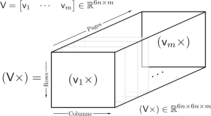
Figure 8: Storage order for the applying the cross product operator to a matrix. A cross product matrix for each column is placed along each page of the dimension 3 tensor.

Algorithm 1 Torsion-Free Coriolis Matrix Algo. for Clusters

0:  $q,\,\overline{v}$

1:  $\mathsf{v}_{0}=\mbox{\boldmath$0$}$

2:  for $i=1$ to $N$ do

3:     $\mathsf{v}_{i}={}^{i}\mathsf{X}_{p(i)}\,\mathsf{v}_{p(i)}+\mathsf{\Phi}_{i}\,\overline{v}{}_{{\tiny J}_{i}}$

4:     $\dot{\mathsf{\Phi}}_{i}=(\mathsf{v}_{i}\times)\mathsf{\Phi}_{i}+\mathring{\mathsf{\Phi}}_{i}$

5:     $\mathsf{I}_{i}^{C}={\rm diag}({\mbox{\boldmath$\mathit{I}$}}_{i_{1}},\ldots,{\mbox{\boldmath$\mathit{I}$}}_{i_{n_{i}}})$

6:     $\mathsf{B}_{i}^{C}=\frac{1}{2}[(\mathsf{v}_{i}\times^{*})\mathsf{I}_{i}+(\mathsf{I}_{i}\mathsf{v}_{i})\,\overline{\!\times\!}{}^{*}\,-\mathsf{I}_{i}(\mathsf{v}_{i}\times)]$

7:  end for

8:  for $j=N$ to $1$ do

9:     $\mathsf{f}_{1}=\mathsf{I}_{j}^{C}\,\dot{\mathsf{\Phi}}_{j}+\mathsf{B}_{j}^{C}\,\mathsf{\Phi}_{j}$

10:     $\mathsf{f}_{2}=\mathsf{I}_{j}^{C}\,\mathsf{\Phi}_{j}$

11:     $\mathsf{f}_{3}=(\mathsf{B}_{j}^{C})^{\top}\mathsf{\Phi}_{j}$

12:     $\overline{C}_{jj}=\mathsf{\Phi}{}_{j}^{\top}\,\mathsf{f}_{1}$

13:     $i=j$

14:     while $p(i)>0$ do

15:        $\mathsf{f}_{1}\!=\!{}^{i}\mathsf{X}_{p(i)}^{\top}\,\mathsf{f}_{1}$; $\mathsf{f}_{2}\!=\!{}^{i}\mathsf{X}_{p(i)}^{\top}\,\mathsf{f}_{2}$;  $\mathsf{f}_{3}\!=\!{}^{i}\mathsf{X}_{p(i)}^{\top}\,\mathsf{f}_{3}$

16:        $i=p(i)$

17:        $\overline{C}_{ij}=\mathsf{\Phi}{}_{i}^{\top}\,\mathsf{f}_{1}$

18:        $\overline{C}_{ji}=(\dot{\mathsf{\Phi}}{}_{i}^{\top}\,\mathsf{f}_{2}+\mathsf{\Phi}{}_{i}^{\top}\mathsf{f}_{3})^{\top}$

19:     end while

20:     $\mathsf{I}_{p(j)}^{C}=\mathsf{I}_{p(j)}^{C}+{}^{j}\mathsf{X}_{p(j)}^{\top}\,\mathsf{I}_{j}^{C}\,{}^{j}\mathsf{X}_{p(j)}$

21:     $\mathsf{B}_{p(j)}^{C}=\mathsf{B}_{p(j)}^{C}+{}^{j}\mathsf{X}_{p(j)}^{\top}\,\mathsf{B}_{j}^{C}\,{}^{j}\mathsf{X}_{p(j)}$

22:  end for

23:  return  $\overline{C}$

The algorithm makes use of dimension 3 tensors (with the dimensions sequentially identified as rows, columns, and pages as in Fig. 8) where we use the symbol $(\cdot)^{\!\top_{\!12}}$ to denote transposing the first two dimensions (rows and columns), and likewise for $(\cdot)^{\!\top_{\!13}}$ and $(\cdot)^{\!\top_{\!23}}$. Deriving the algorithm follows the same conceptual approach as in [6], but with the extra book keeping and conventions required for working with tensors. For example, multiplication between a matrix and a dimension 3 tensor is given by:

$$(A\mathcal{B})_{ijk}=\sum_{\ell}A_{i\ell}\mathcal{B}_{\ell jk},$$

with multiplication between a dimension 3 tensor and a matrix given by:

$$(\mathcal{A}B)_{ijk}=\sum_{\ell}\mathcal{A}_{i\ell k}B_{\ell j}$$

so that, in either case, multiplication occurs page-by-page for the tensor. We adopt the same conventions as in [67] where for any $\mathsf{\Phi}_{i}\in\mathbb{R}^{6n_{i}\times d_{i}}$ we construct $(\mathsf{\Phi}_{i}\times)\in\mathbb{R}^{6n_{i}\times 6n_{i}\times d_{i}}$ by considering the usual cross product $(~{}\times)$ for each column of $\mathsf{\Phi}_{i}$ and stacking the results along pages (Fig. 8).

To arrive at the computational structure in Algo. 2, we employ the following identities when $j$ and $k$ are related:

$$\frac{\partial\mathsf{B}_{k}^{C}}{\partial\overline{v}{}_{{\tiny J}_{j}}} =\sum_{\ell\succeq\lceil jk\rceil}{}^{\ell}\mathsf{X}_{k}^{\top}\,\mathsf{B}\left(\mathsf{I}_{\ell},\,{}^{\ell}\mathsf{X}_{j}\mathsf{\Phi}_{j}\right)\,{}^{\ell}\mathsf{X}_{k}$$ (24)

$$={}^{\lceil jk\rceil}\mathsf{X}_{k}^{\top}\,\mathsf{B}\left(\mathsf{I}_{\lceil jk\rceil}^{C},\,{}^{\lceil jk\rceil}\mathsf{X}_{j}\mathsf{\Phi}_{j}\right)\,{}^{\lceil jk\rceil}\mathsf{X}_{k}$$ (25)

and

$$\frac{\partial\dot{\mathsf{\Phi}}_{k}}{\partial\overline{v}{}_{{\tiny J}_{j}}}=\mathsf{\Phi}_{j}\times\mathsf{\Phi}_{k}+\frac{\partial\mathring{\mathsf{\Phi}}_{k}}{\partial\overline{v}{}_{{\tiny J}_{j}}}~{}~{}~{}(j\preceq k)$$ (26)

where partial derivatives w.r.t. the different components of $\overline{v}{}_{{\tiny J}_{j}}$ are stacked along pages.

In arranging the computations for recursive implementation, we employ that for matrices $\mathsf{V}$ and $\mathsf{W}$ and inertia $\mathsf{I}$ with matched row-dimensions, we have [67, Table 3]:

$$\mathsf{B}(\mathsf{I},\mathsf{V})^{\!\top_{\!12}}\,\mathsf{W} =(-\mathsf{B}(\mathsf{I},\mathsf{W})^{\!\top_{\!12}}\,\mathsf{V})^{\!\top_{\!23}}$$ (27)

$$\mathsf{B}(\mathsf{I},\mathsf{V})\mathsf{W} =\left(\mathsf{B}(\mathsf{I},\mathsf{W})\mathsf{V}+\mathsf{I}\,(\mathsf{W}\times)\mathsf{V}\right)^{\!\top_{\!23}}$$ (28)

We omit the full derivation here as, again, it conceptually follows the one for the simplified case in [6], but with extra tediousness for tracking tensor storage.

Overall, Algo. 2 has computational complexity $\mathcal{O}(Nd^{2})$ when applied to a fixed library of clusters. The first for loop (Lines 1-4) has complexity $\mathcal{O}(N)$. The main for loop (Lines 5-32) executes $N$ times, while the nested while loops (Lines 10-30 and 13-27) execute at most $d$ times each. The assignments on Lines 15-17 give the symmetric parts of the generalized Christoffel symbols, while the two if statements (Lines 18 and 21) cover cases where the basis vector fields do not commute, as would be signified by a quantity $\mathcal{D}_{i}=\frac{\partial\mathring{\mathsf{\Phi}}_{i}}{\partial\overline{v}{}_{{\tiny J}_{i}}}$ lacking symmetry in its 2-3 dimensions.

Algorithm 2 Generalized Christoffel Symbols for Clusters

0:  $q$

1:  for $i=1$ to $N$ do

2:     $\mathsf{I}_{i}^{C}={\rm diag}({\mbox{\boldmath$\mathit{I}$}}_{i_{1}},\ldots,{\mbox{\boldmath$\mathit{I}$}}_{i_{n_{i}}})$

3:     $\mathcal{D}_{i}=\left(\frac{\partial\mathring{\mathsf{\Phi}}_{i}}{\partial\overline{v}{}_{{\tiny J}_{i}}}\right)^{\!\top_{\!23}}$

4:  end for

5:  for $k=N$ to $1$ do

6:     $\mathcal{B}=\mathsf{B}(\mathsf{I}^{C}_{k},\mathsf{\Phi}_{k})$

7:     $\mathcal{F}_{3}=\mathsf{I}_{k}^{C}\,\mathcal{D}_{k}$

8:     $\mathsf{f}_{4}=\mathsf{I}_{k}^{C}\,\mathsf{\Phi}_{k}$

9:     $j=k$

10:     while $j>0$ do

11:        $\mathcal{F}_{1}=\mathcal{B}\,\mathsf{\Phi}_{j}$, $\mathcal{F}_{2}=\mathcal{B}^{\top}\,\mathsf{\Phi}_{j}$

12:        $i=j$

13:        while $i>0$ do

14:           $\mathcal{A}_{1}=\mathsf{\Phi}_{i}^{\top}\mathcal{F}_{1}$, $\mathcal{A}_{2}=\left(\mathsf{\Phi}_{i}^{\top}\mathcal{F}_{2}\right)^{\!\top_{\!12}}$, $\mathcal{A}_{3}=-(\mathcal{A}_{2})^{\!\top_{\!13}}$

15:           $\overline{\Gamma}{}_{ijk}=\mathcal{A}_{1}$, $\overline{\Gamma}{}_{ikj}=\left(\mathcal{A}_{1}\right)^{\top_{\!23}}$

16:           $\overline{\Gamma}{}_{jik}=\mathcal{A}_{2}$, $\overline{\Gamma}{}_{jki}=\left(\mathcal{A}_{2}\right)^{\top_{\!23}}$

17:           $\overline{\Gamma}{}_{kij}=\mathcal{A}_{3}$, $\overline{\Gamma}{}_{kji}=\left(\mathcal{A}_{3}\right)^{\top_{\!23}}$

18:           if $i=j$ then

19:              $\overline{\Gamma}{}_{kii}=\mathcal{A}_{3}+\mathsf{f}_{4}^{\top}\mathcal{D}_{i}$

20:           end if

21:           if $j=k$ then

22:              $\overline{\Gamma}{}_{ijj}=\mathcal{A}_{1}+\mathsf{\Phi}_{i}^{\top}\mathcal{F}_{3}$

23:              $\mathcal{F}_{3}={}^{i}\mathsf{X}_{p(i)}^{\top}\mathcal{F}_{3}$

24:           end if

25:           $\mathcal{F}_{1}={}^{i}\mathsf{X}_{p(i)}^{\top}\mathcal{F}_{1}$, $\mathcal{F}_{2}={}^{i}\mathsf{X}_{p(i)}^{\top}\mathcal{F}_{2}$

26:           $i=p(i)$

27:        end while

28:        $\mathcal{B}={}^{j}\mathsf{X}_{p(j)}^{\top}\,\mathcal{B}\,{}^{j}\mathsf{X}_{p(j)}$, $\mathsf{f}_{4}={}^{j}\mathsf{X}_{p(j)}^{\top}\mathsf{f}_{4}$

29:        $j=p(j)$

30:     end while

31:     $\mathsf{I}_{p(k)}^{C}=\mathsf{I}_{p(k)}^{C}+{}^{k}\mathsf{X}_{p(k)}^{\top}\,\mathsf{I}_{k}^{C}\,{}^{k}\mathsf{X}_{p(k)}$

32:  end for

33:  return  $\overline{\Gamma}{}$

VI-D Computation via Differentiation

In the interest of completeness, we close this section by describing a way to obtain the Christoffel-consistent Coriolis matrix via derivative calculations applied to the Coriolis and centripetal terms. When working with generalized coordinates, one can compute $C^{\scalebox{0.5}{\scalerel*{\stackinset{c}{-.125pt}{c}{}{\scalebox{0.5}{\color[rgb]{1,1,1}{$\bigstar$}}}{$\bigstar$}}{\bigstar}}}$ via:

$$[C^{\scalebox{0.5}{\scalerel*{\stackinset{c}{-.125pt}{c}{}{\scalebox{0.5}{\color[rgb]{1,1,1}{$\bigstar$}}}{$\bigstar$}}{\bigstar}}}]_{ik}=\frac{1}{2}\frac{\partial[C(q,\dot{q})\dot{q}]_{i}}{\partial\dot{q}^{k}}$$

However, this formula can break down when working with generalized speeds, since the generalized Christoffel symbols are no longer guaranteed to be symmetric in their (2,3) indices.

Indeed, considering the derivatives of $C(q,v)v$ w.r.t. $v$ gives:

$$\frac{\partial[C(q,v)v]_{i}}{\partial v^{k}}=2\,\Gamma^{\scalebox{0.5}{\scalerel*{\stackinset{c}{-.125pt}{c}{}{\scalebox{0.5}{\color[rgb]{1,1,1}{$\bigstar$}}}{$\bigstar$}}{\bigstar}}}_{i(jk)}v^{j}$$

As a result, using (9), we have that:

$$C_{ik}^{\scalebox{0.5}{\scalerel*{\stackinset{c}{-.125pt}{c}{}{\scalebox{0.5}{\color[rgb]{1,1,1}{$\bigstar$}}}{$\bigstar$}}{\bigstar}}} =\frac{1}{2}\frac{\partial[C(q,v)v]_{i}}{\partial v^{k}}+\frac{1}{2}s_{ijk}v^{j}$$ (29)

$$=\frac{1}{2}\frac{\partial[C(q,v)v]_{i}}{\partial v^{k}}+\frac{1}{2}H_{i\ell}s_{jk}^{\ell}v^{j}$$ (30)

$$=\frac{1}{2}\frac{\partial[C(q,v)v]_{i}}{\partial v^{k}}+\frac{1}{2}H_{i\ell}X^{\ell}\cdot[X_{j},X_{k}]v^{j}$$ (31)

where $X^{1},\ldots,X^{n}$ gives the basis dual to $X_{1},\ldots,X_{n}$. In this regard, one can construct the Christoffel-consistent Coriolis matrix via derivatives of the EOM when working with generalized coordinates, but such a construction requires a correction factor via the structure constants when working with generalized speeds.

For example, for open-chain robots with joint models satisfying $\mathring{\bm{\Phi}}_{i}=0$, we can compute (31) as follows. For general open-chain mechanisms, the structure constants $X^{\ell}\cdot[X_{j},X_{k}]$ are only nonzero when $\ell$, $j$, and $k$ all belong to the same joint (since the motions of different joints will commute). Considering the columns of $\bm{\Phi}_{i}$ as a partial basis for $\mathbb{R}^{6}$ we complete the basis via any complimentary matrix $\bm{\Phi}_{i}^{c}$ such that $[\bm{\Phi}_{i}~{}\bm{\Phi}_{i}^{c}]\in\mathbb{R}^{6\times 6}$ is full rank. Defining $[\bm{\Psi}_{i}~{}\bm{\Psi}_{i}^{c}]=[\bm{\Phi}_{i}~{}\bm{\Phi}_{i}^{c}]^{-\top}$ we have that $\bm{\Psi}_{i}^{\top}\bm{\Phi}_{i}=\mathbf{1}$ via construction. We will use these dual vectors $\bm{\Psi}_{i}$ to compute (31).

Consider local blocks:

$$K_{i}(q,v)=\mathbf{\Psi}_{i}^{\top}(\mathbf{\Phi}_{i}v^{J_{i}})\times\mathbf{\Phi}_{i}$$

where, again, $v^{J_{i}}$ is the subvector of $v$ corresponding to the velocity components of joint $i$. We stack these $K_{i}$ matrices into a block diagonal matrix $K={\rm BlockDiag}(K_{1},\ldots,K_{N})$, which then enables implementing (31) via

$$C^{\scalebox{0.5}{\scalerel*{\stackinset{c}{-.125pt}{c}{}{\scalebox{0.5}{\color[rgb]{1,1,1}{$\bigstar$}}}{$\bigstar$}}{\bigstar}}}(q,v)=\frac{1}{2}\left[\frac{\partial C(q,v)v}{\partial v}+H(q)K(q,v)\right]$$ (32)

This approach might be more straightforward for those who have access to an efficient auto-differentiation package (e.g., such as is part of CasADi [68]).

Remark 9.

Eq. 32 also helps to link algorithms for the Coriolis matrix [6] with those that calculate sensitivities of the inverse dynamics

$${\rm ID}(q,v,\dot{v})=H(q)\dot{v}+C(q,v)v+g(q)$$

with respect to state $(q,v)$ (see, e.g., [69, 70, 71, 72, 31]).

Recent results have noted the promise of carrying out these (and other) dynamics computations using insights from geometric algebra [72, 73, 74]. The detail in (19) and (21) may provide additional clues, in particular, to further accelerate those computations for sensitivity analysis [72].

VII Conclusions

This paper has provided a comprehensive overview of the link between Coriolis factorizations and affine connections on the configuration manifold. Analysis of the contorsion tensor (measuring the difference from the Riemannian connection) proved that there is a unique factorization satisfying the skew property when $n\leq 2$, but an infinity of options when $n\geq 3$. Despite this flexibility, the Coriolis matrix associated with the Riemannian connection (and therefore associated with the Christoffel symbols) inherits an additional property of being torsion-free, which we have shown avoids excess twisting of trajectories in passivity-based control. While the presence of torsion does not affect the Lyapunov argument in this case, it leads to oscillations in the control output which could incite unmodeled high-frequency vibrations in mechanical systems. This motivation led us to address how to compute the Christoffel-consistent Coriolis matrix for complex mechanical systems, wherein our results on induced factorizations played a central role. For open-chain mechanical systems, this Coriolis matrix can be computed with computational complexity $O(Nd)$, which promotes its use in control strategies for systems such as humanoids and quadruped robots. Extensions demonstrated how these constructions can be applied for computation the Coriolis matrix and generalized symbols of the Riemannian connection for systems with local loop closures. These algorithms may be considered for other applications beyond passivity-based control (e.g., when taking covariant derivatives in other contexts).

Future work will focus on testing the theory with non-trivial robot models for passivity-based tracking control and whole-body control.

References

- [1] M. P. Do Carmo, Riemannian geometry. Birkhäuser, 1992.
- [2] M. Bjerkeng and K. Y. Pettersen, “A new coriolis matrix factorization,” in 2012 IEEE International Conference on Robotics and Automation. IEEE, 2012, pp. 4974–4979.
- [3] J.-J. E. Slotine and W. Li, “On the adaptive control of robot manipulators,” The International Journal of Robotics Research, vol. 6, no. 3, pp. 49–59, 1987.
- [4] R. Ortega and M. W. Spong, “Adaptive motion control of rigid robots: A tutorial,” Automatica, vol. 25, no. 6, pp. 877–888, 1989.
- [5] B. Siciliano, L. Sciavicco, L. Villani, and G. Oriolo, Robotics: modelling, planning and control. Springer London, 2009.
- [6] S. Echeandia and P. M. Wensing, “Numerical methods to compute the coriolis matrix and christoffel symbols for rigid-body systems,” Journal of Computational and Nonlinear Dynamics, vol. 16, no. 9, 2021.
- [7] D. E. Orin, R. McGhee, M. Vukobratović, and G. Hartoch, “Kinematic and kinetic analysis of open-chain linkages utilizing newton-euler methods,” Mathematical Biosciences, vol. 43, no. 1-2, pp. 107–130, 1979.
- [8] Y. Stepanenko and M. Vukobratović, “Dynamics of articulated open-chain active mechanisms,” Mathematical Biosciences, vol. 28, no. 1-2, pp. 137–170, 1976.
- [9] J. Y. S. Luh, M. W. Walker, and R. P. C. Paul, “On-Line Computational Scheme for Mechanical Manipulators,” Journal of Dynamic Systems, Measurement, and Control, vol. 102, no. 2, pp. 69–76, 06 1980.
- [10] J.-J. Slotine, “Putting physics in control-the example of robotics,” IEEE Control Systems Magazine, vol. 8, no. 6, pp. 12–18, 1988.
- [11] M. Takegaki and S. Arimoto, “A New Feedback Method for Dynamic Control of Manipulators,” Journal of Dynamic Systems, Measurement, and Control, vol. 103, no. 2, pp. 119–125, 06 1981.
- [12] D. Koditschek, “Natural motion for robot arms,” in IEEE Conference on Decision and Control, 1984, pp. 733–735.
- [13] R. Ortega, J. A. L. Perez, P. J. Nicklasson, and H. J. Sira-Ramirez, Passivity-based control of Euler-Lagrange systems: mechanical, electrical and electromechanical applications. Springer Science & Business Media, 2013.
- [14] D. Pucci, F. Romano, and F. Nori, “Collocated adaptive control of underactuated mechanical systems,” IEEE Transactions on Robotics, vol. 31, no. 6, pp. 1527–1536, 2015.
- [15] A. Dietrich, X. Wu, K. Bussmann, C. Ott, A. Albu-Schäffer, and S. Stramigioli, “Passive hierarchical impedance control via energy tanks,” IEEE Robotics and Automation Letters, vol. 2, no. 2, pp. 522–529, 2016.
- [16] N. Chopra, M. Fujita, R. Ortega, and M. W. Spong, “Passivity-based control of robots: Theory and examples from the literature,” IEEE Control Systems Magazine, vol. 42, no. 2, pp. 63–73, 2022.
- [17] R. Anderson and M. Spong, “Bilateral control of teleoperators with time delay,” IEEE Transactions on Automatic Control, vol. 34, no. 5, pp. 494–501, 1989.
- [18] G. Niemeyer and J.-J. Slotine, “Stable adaptive teleoperation,” IEEE Journal of oceanic engineering, vol. 16, no. 1, pp. 152–162, 1991.
- [19] K. M. Lynch and F. C. Park, Modern robotics. Cambridge University Press, 2017.
- [20] G. D. Niemeyer, “Computational algorithms for adaptive robot control,” Master’s thesis, MIT, 1990.
- [21] G. Niemeyer and J.-J. E. Slotine, “Performance in adaptive manipulator control,” The International Journal of Robotics Research, vol. 10, no. 2, pp. 149–161, 1991.
- [22] H.-C. Lin, T.-C. Lin, and K. Yae, “On the skew-symmetric property of the newton-euler formulation for open-chain robot manipulators,” in American Control Conference, vol. 3, 1995, pp. 2322–2326.
- [23] S. R. Ploen, “A skew-symmetric form of the recursive newton-euler algorithm for the control of multibody systems,” in Proceedings of the 1999 American Control Conference (Cat. No. 99CH36251), vol. 6. IEEE, 1999, pp. 3770–3773.
- [24] T. I. Fossen, Nonlinear modelling and control of underwater vehicles. Universitetet i Trondheim (Norway), 1991.
- [25] I. Schjølberg, Modeling and control of underwater robotic systems. Norwegian University of Science and Technology, 1996.
- [26] H. Wang and Y. Xie, “Passivity based adaptive jacobian tracking for free-floating space manipulators without using spacecraft acceleration,” Automatica, vol. 45, no. 6, pp. 1510–1517, 2009.
- [27] ——, “On the recursive adaptive control for free-floating space manipulators,” Journal of Intelligent & Robotic Systems, vol. 66, no. 4, pp. 443–461, 2012.
- [28] A. D. Luca, A. Albu-Schaffer, S. Haddadin, and G. Hirzinger, “Collision detection and safe reaction with the DLR-III lightweight manipulator arm,” in IEEE/RSJ International Conference on Intelligent Robots and Systems, Oct 2006, pp. 1623–1630.
- [29] G. Bledt, P. M. Wensing, S. Ingersoll, and S. Kim, “Contact model fusion for event-based locomotion in unstructured terrains,” in 2018 IEEE International Conference on Robotics and Automation (ICRA), 2018, pp. 4399–4406.
- [30] A. De Luca and L. Ferrajoli, “A modified Newton-Euler method for dynamic computations in robot fault detection and control,” in IEEE International Conference on Robotics and Automation, May 2009, pp. 3359–3364.
- [31] J. Carpentier, G. Saurel, G. Buondonno, J. Mirabel, F. Lamiraux, O. Stasse, and N. Mansard, “The Pinocchio C++ library: A fast and flexible implementation of rigid body dynamics algorithms and their analytical derivatives,” in 2019 IEEE/SICE International Symposium on System Integration (SII). IEEE, 2019, pp. 614–619.
- [32] H. Wang, “Recursive composite adaptation for robot manipulators,” Journal of Dynamic Systems, Measurement, and Control, vol. 135, no. 2, p. 021010, 2013.
- [33] B. Henze, M. A. Roa, and C. Ott, “Passivity-based whole-body balancing for torque-controlled humanoid robots in multi-contact scenarios,” The International Journal of Robotics Research, vol. 35, no. 12, pp. 1522–1543, 2016.
- [34] J. Englsberger, A. Dietrich, G.-A. Mesesan, G. Garofalo, C. Ott, and A. O. Albu-Schäffer, “MPTC-modular passive tracking controller for stack of tasks based control frameworks,” 2020.
- [35] V. Kurtz, P. M. Wensing, and H. Lin, “Approximate simulation for template-based whole-body control,” IEEE Robotics and Automation Letters, vol. 6, no. 2, pp. 558–565, 2020.
- [36] A. Escande, N. Mansard, and P.-B. Wieber, “Hierarchical quadratic programming: Fast online humanoid-robot motion generation,” The International Journal of Robotics Research, vol. 33, no. 7, pp. 1006–1028, 2014.
- [37] S. Kuindersma, R. Deits, M. Fallon, A. Valenzuela, H. Dai, F. Permenter, T. Koolen, P. Marion, and R. Tedrake, “Optimization-based locomotion planning, estimation, and control design for the atlas humanoid robot,” Autonomous robots, vol. 40, no. 3, pp. 429–455, 2016.
- [38] G. Garofalo, C. Ott, and A. Albu-Schäffer, “On the closed form computation of the dynamic matrices and their differentiations,” in IEEE/RSJ International Conference on Intelligent Robots and Systems, 2013, pp. 2364–2359.
- [39] G. I. Boutselis and E. Theodorou, “Discrete-time differential dynamic programming on lie groups: Derivation, convergence analysis, and numerical results,” IEEE Transactions on Automatic Control, vol. 66, no. 10, pp. 4636–4651, 2020.
- [40] H. Mishra, G. Garofalo, A. M. Giordano, M. De Stefano, C. Ott, and A. Kugi, “Reduced euler-lagrange equations of floating-base robots: Computation, properties, & applications,” IEEE Transactions on Robotics, vol. 39, no. 2, pp. 1439–1457, 2022.
- [41] J. Welde, M. D. Kvalheim, and V. Kumar, “The role of symmetry in constructing geometric flat outputs for free-flying robotic systems,” arXiv preprint arXiv:2209.11869, 2022.
- [42] A. D. Lewis and R. M. Murray, “Configuration controllability of simple mechanical control systems,” SIAM Journal on control and optimization, vol. 35, no. 3, pp. 766–790, 1997.
- [43] N. Jaquier and T. Asfour, “Riemannian geometry as a unifying theory for robot motion learning and control,” arXiv preprint arXiv:2209.15539, 2022.
- [44] F. Bullo and A. D. Lewis, Geometric control of mechanical systems: modeling, analysis, and design for simple mechanical control systems. Springer Science & Business Media, 2004, vol. 49.
- [45] A. Van der Schaft, L2-gain and passivity techniques in nonlinear control. Springer, 2017.
- [46] R. Reyes-Báez, P. Borja, A. van der Schaft, and B. Jayawardhana, “Virtual mechanical systems: An energy-based approach,” in Congreso Nacional de Control Automático, 2019.
- [47] G. Hamel, “Über nichtholonome systeme,” Mathematische Annalen, vol. 92, no. 1, pp. 33–41, 1924. [Online]. Available: https://doi.org/10.1007/BF01448428
- [48] K. R. Ball, D. V. Zenkov, and A. M. Bloch, “Variational structures for hamel’s equations and stabilization,” IFAC Proceedings Volumes, vol. 45, no. 19, pp. 178–183, 2012.
- [49] A. Müller, “Hamel’s equations and geometric mechanics of constrained and floating multibody and space systems,” Proceedings of the Royal Society A, vol. 479, no. 2273, p. 20220732, 2023.
- [50] J. Nash, “The imbedding problem for riemannian manifolds,” Annals of mathematics, pp. 20–63, 1956.
- [51] M. Nakahara, Geometry, topology and physics. CRC Press, 2003.
- [52] V. I. Arnol’d, Mathematical methods of classical mechanics. Springer Science & Business Media, 2013, vol. 60.
- [53] M. Spivak, “Comprehensive introduction to differential geometry,(vol. 2, 3rd edn),” 2005.
- [54] C. G. Atkeson, C. H. An, and J. M. Hollerbach, “Estimation of inertial parameters of manipulator loads and links,” The International Journal of Robotics Research, vol. 5, no. 3, pp. 101–119, 1986.
- [55] J. Yuan and B. Yuan, “Recursive computation of the slotine-li regressor,” in American Control Conference, vol. 3, 1995, pp. 2327–2331.
- [56] B. Siciliano and J.-J. E. Slotine, “A general framework for managing multiple tasks in highly redundant robotic systems,” in International Conference on Advanced Robotics, vol. 2, 1991, pp. 1211–1216.
- [57] J.-J. E. Slotine, “Modular stability tools for distributed computation and control,” International Journal of Adaptive Control and Signal Processing, vol. 17, no. 6, pp. 397–416, 2003.
- [58] F. Bullo and R. M. Murray, “Tracking for fully actuated mechanical systems: a geometric framework,” Automatica, vol. 35, no. 1, pp. 17–34, 1999.
- [59] R. Featherstone, Rigid body dynamics algorithms. Springer, 2014.
- [60] P. M. Wensing, S. Kim, and J.-J. E. Slotine, “Linear matrix inequalities for physically consistent inertial parameter identification: A statistical perspective on the mass distribution,” IEEE Robotics and Automation Letters, vol. 3, no. 1, pp. 60–67, 2017.
- [61] P. M. Wensing, “spatial_v2_extended: CoriolisMatrix.m,” https://github.com/ROAM-Lab-ND/spatial_v2_extended, 2022, see v3/dynamics/CoriolisMatrix.m from commit e1be717 (link).
- [62] P. M. Wensing et al., “Christoffel-consistent factorization and covariant derivatives,” https://github.com/stack-of-tasks/pinocchio/discussions/1663, 2022, (link).
- [63] A. Jain, “Multibody graph transformations and analysis: part ii: closed-chain constraint embedding,” Nonlinear dynamics, vol. 67, pp. 2153–2170, 2012.
- [64] S. Kumar, K. A. v. Szadkowski, A. Mueller, and F. Kirchner, “An analytical and modular software workbench for solving kinematics and dynamics of series-parallel hybrid robots,” Journal of Mechanisms and Robotics, vol. 12, no. 2, p. 021114, 2020.
- [65] M. Chignoli, N. Adrian, S. Kim, and P. M. Wensing, “Recursive rigid-body dynamics algorithms for systems with kinematic loops,” arXiv preprint, arXiv:2311.13732, 2023.
- [66] P. M. Wensing, “spatial_v2_extended: Christoffel_tens.m,” https://github.com/ROAM-Lab-ND/spatial_v2_extended, 2023, see v3/dynamics/Christoffel_tens.m from commit fe3e76c (link).
- [67] S. Singh, R. P. Russell, and P. M. Wensing, “On second-order derivatives of rigid-body dynamics: Theory & implementation,” arXiv preprint arXiv:2302.06001, 2023.
- [68] J. A. Andersson, J. Gillis, G. Horn, J. B. Rawlings, and M. Diehl, “Casadi: a software framework for nonlinear optimization and optimal control,” Mathematical Programming Computation, vol. 11, pp. 1–36, 2019.
- [69] A. Jain and G. Rodriguez, “Linearization of manipulator dynamics using spatial operators,” IEEE transactions on Systems, Man, and Cybernetics, vol. 23, no. 1, pp. 239–248, 1993.
- [70] S. Singh, R. P. Russell, and P. M. Wensing, “Efficient analytical derivatives of rigid-body dynamics using spatial vector algebra,” IEEE Robotics and Automation Letters, vol. 7, no. 2, pp. 1776–1783, 2022.
- [71] M. Bos, S. Traversaro, D. Pucci, and A. Saccon, “Efficient geometric linearization of moving-base rigid robot dynamics,” Journal of Geometric Mechanics, vol. 14, no. 4, pp. 507–543, 2022.
- [72] G. Sun and Y. Ding, “An analytical method for sensitivity analysis of rigid multibody system dynamics using projective geometric algebra,” Journal of Computational and Nonlinear Dynamics, vol. 18, no. 11, 2023.
- [73] ——, “High-order inverse dynamics of serial robots based on projective geometric algebra,” Multibody System Dynamics, pp. 1–26, 2023.
- [74] T. Löw and S. Calinon, “Geometric algebra for optimal control with applications in manipulation tasks,” IEEE Transactions on Robotics, 2023.